1. A mail-order computer business has six telephone lines. Let X ...
1. A mail-order computer business has six telephone lines. Let X ...
1. A mail-order computer business has six telephone lines. Let X ...

Create successful ePaper yourself
Turn your PDF publications into a flip-book with our unique Google optimized e-Paper software.
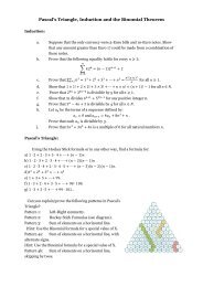
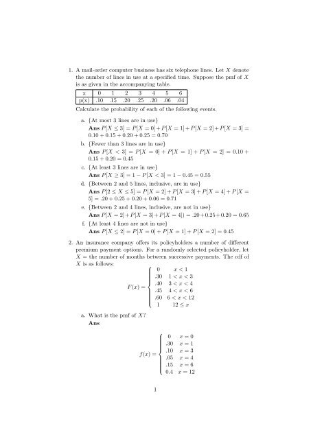
<strong>1.</strong> A <strong>mail</strong>-<strong>order</strong> <strong>computer</strong> <strong>business</strong> <strong>has</strong> <strong>six</strong> <strong>telephone</strong> <strong>lines</strong>. <strong>Let</strong> X denote<br />
the number of <strong>lines</strong> in use at a specified time. Suppose the pmf of X<br />
is as given in the accompanying table.<br />
x 0 1 2 3 4 5 6<br />
p(x) .10 .15 .20 .25 .20 .06 .04<br />
Calculate the probability of each of the following events.<br />
a. {At most 3 <strong>lines</strong> are in use}<br />
Ans P [X ≤ 3] = P [X = 0] + P [X = 1] + P [X = 2] + P [X = 3] =<br />
0.10 + 0.15 + 0.20 + 0.25 = 0.70<br />
b. {Fewer than 3 <strong>lines</strong> are in use}<br />
Ans P [X < 3] = P [X = 0] + P [X = 1] + P [X = 2] = 0.10 +<br />
0.15 + 0.20 = 0.45<br />
c. {At least 3 <strong>lines</strong> are in use}<br />
Ans P [X ≥ 3] = 1 − P [X < 3] = 1 − 0.45 = 0.55<br />
d. {Between 2 and 5 <strong>lines</strong>, inclusive, are in use}<br />
Ans P [2 ≤ X ≤ 5] = P [X = 2] + P [X = 3] + P [X = 4] + P [X =<br />
5] = .20 + 0.25 + 0.20 + 0.06 = 0.71<br />
e. {Between 2 and 4 <strong>lines</strong>, inclusive, are not in use}<br />
Ans P [X = 2]+P [X = 3]+P [X = 4]) = .20+0.25+0.20 = 0.65<br />
f. {At least 4 <strong>lines</strong> are not in use}<br />
Ans P [X ≤ 2] = P [X = 0] + P [X = 1] + P [X = 2] = 0.45<br />
2. An insurance company offers its policyholders a number of different<br />
premium payment options. For a randomly selected policyholder, let<br />
X = the number of months between successive payments. The cdf of<br />
X is as follows:<br />
⎧<br />
⎪⎨<br />
F (x) =<br />
a. What is the pmf of X?<br />
Ans<br />
⎪⎩<br />
⎪⎨<br />
f(x) =<br />
0 x < 1<br />
.30 1 < x < 3<br />
.40 3 < x < 4<br />
.45 4 < x < 6<br />
.60 6 < x < 12<br />
1 12 ≤ x<br />
1<br />
⎧<br />
⎪⎩<br />
0 x = 0<br />
.30 x = 1<br />
.10 x = 3<br />
.05 x = 4<br />
.15 x = 6<br />
0.4 x = 12
. Using just the cdf, compute P (3 < X < 6) and P (4 < X).<br />
Ans<br />
P (3 < X < 6) = P [X = 3, 4, 6] = 0.1 + 0.05 + 0.25 = 0.3<br />
P (4 < X) = P [X = 6, 12] = 0.55.<br />
3. An appliance dealer sells three different models of upright freezers<br />
having 13.5, 15.9, and 19.1 cubic feet of storage space, respectively.<br />
<strong>Let</strong> X = the amount of storage space purc<strong>has</strong>ed by the next customer<br />
to buy a freezer. Suppose that X <strong>has</strong> probability mass function<br />
x 13.5 15.9 19.1<br />
p(x) .2 .5 .3<br />
a. Compute E(X), E(X 2 ), and V (X).<br />
Ans<br />
E(X) = 16.38, E(X 2 ) = 272.298, and V (X) = 3.9936<br />
b. If the price of a freezer having capacity X cubic feet is 25X −8.5,<br />
what is the expected price paid by the next customer to buy a<br />
freezer?<br />
Ans<br />
E[25X − 8.5] = (25)E[X] − 8.5 = 401,<br />
c. What is the variance of the price 25X − 8.5 paid by the next<br />
customer?<br />
Ans<br />
V [25X − 8.5] = [(25) 2 ]V [X] = 2496<br />
d. Suppose that while the rated capacity of a freezer is X, the actual<br />
capacity is h(X) = X − .01X 2 . What is the expected actual<br />
capacity of the freezer purc<strong>has</strong>ed by the next customer?<br />
Ans<br />
E[h(X)] = E[X − .01X 2 ] = E[X] − (.01)E[X 2 ] = 13.66.<br />
4. A chemical supply company currently <strong>has</strong> in stock 100 Kg of a certain<br />
chemical, which it sells to customers 5 Kg lots. <strong>Let</strong> X = the number<br />
of lots <strong>order</strong>ed by a randomly chosen customer, and suppose that X<br />
<strong>has</strong> pmf<br />
x 1 2 3 4<br />
p(x) .2 .4 .3 .1<br />
Compute E(X) and V (X). Then compute the expected number of<br />
Kg’s left after the next customer’s <strong>order</strong> is shipped, and the variance<br />
of the number of Kg’s left.<br />
Ans<br />
2
E[X] = (1 × 0.2) + (2 × 0.4) + (3 × 0.3) + (4 × 0.1)<br />
= 0.2 + 0.8 + 0.9 + 0.4 = 2.3<br />
V [X] = E[X 2 ]−(E[X]) 2 = (1×0.2)+(4×0.4)+(9×0.3)+(16×0.1)−2.3 2<br />
= (0.2 + <strong>1.</strong>6 + 2.7 + <strong>1.</strong>6) − 2.3 2 = 0.81<br />
The required r.v. is Y = 100 − 5X, therefore,<br />
E[Y ] = 100 − 5 × E[X] = 100 − 5 × 2.3 = 100 − 1<strong>1.</strong>5 = 88.5<br />
V [Y ] = V [100 − 5 × V [X]] = (5 2 ) × V [X] = 20.25<br />
5. When circuit boards used in the manufacture of compact disc players<br />
are tested, the long-run percentage of defectives is 5%. <strong>Let</strong> X = the<br />
number of defective boards in a random sample of size n = 25, so<br />
X ∼ BIN(25, 0.05).<br />
(a) Determine P (X ≤ 2)<br />
(b) Determine P (X ≥ 5)<br />
(c) Determine P (1 ≤ X ≤ 4)<br />
(d) What is the probability that none of the 25 boards are defective?<br />
(e) Calculate the expected value and standard deviation of X.<br />
(a) Determine P [X ≤ 2].<br />
=<br />
10<br />
0<br />
P [X ≤ 2] =<br />
<br />
(0.5) 0 0.5 10 +<br />
=<br />
(b) Determine P [X ≥ 5].<br />
2<br />
x=0<br />
10<br />
x<br />
10<br />
1<br />
<br />
(0.5) x [1 − 0.5] 10−x<br />
<br />
(0.5) 1 0.5 9 <br />
10<br />
+<br />
2<br />
10!<br />
0!(10 − 0)! [0.000976562]<br />
10!<br />
+<br />
1!(10 − 1)! [0.000976562]<br />
10!<br />
+<br />
2!(10 − 2)! [0.000976252]<br />
= (1 + 10 + 45) × 0.000976562<br />
= 56 × 0.000976562 = 0.0546875<br />
3<br />
<br />
(0.5) 2 0.5 8
P [X ≤ 2] =<br />
=<br />
10<br />
x=5<br />
10<br />
x<br />
<br />
(0.5) x [1 − 0.5] 10−x<br />
10!<br />
5!(10 − 5)! [0.000976562]<br />
10!<br />
+<br />
6!(10 − 6)! [0.000976562]<br />
10!<br />
+<br />
7!(10 − 7)! [0.000976252]<br />
=<br />
10!<br />
8!(10 − 8)! [0.000976562]<br />
10!<br />
+<br />
9!(10 − 9)! [0.000976562]<br />
10!<br />
+<br />
10!(10 − 10)! [0.000976252]<br />
= (252 + 210 + 120 + 45 + 10 + 1) × 0.000976562<br />
(c) Determine P [1 ≤ X ≤ 4].<br />
Ans Required probability:<br />
= 0.6230469<br />
(1 + 10 + 45 + 120 + 210) × 0.000976562<br />
= 386 × 0.000976562<br />
= 0.3769531<br />
Note that we could also have arrived at the same answer, without<br />
computing binomial coefficients, by observing that,<br />
P [1 ≤ X ≤ 4] = P [X = 0] + [1 − P [X ≥ 5]]<br />
= 1 + 0.000976562 − 0.6230469 = 0.3769<br />
(d) What is the probability that none of the 10 boards are defective?<br />
Ans This is the probability<br />
P [X = 0] = 0.0009765<br />
(e) Calculate the expected value and standard deviation of X.<br />
Ans We know that any Binomial r.v. can be defined as the<br />
sum of independent Bernoulli trials, i.e., if X ∼ BIN(n, p), then<br />
4
X = n<br />
i=1 Xi, where each Xi ∼ BIN(1, p), (or Bernoulli with<br />
parameter p - a r.v taking value 1 with probability p and 0 with<br />
pr. 1 − p).<br />
Therefore<br />
=<br />
E[X] = E[<br />
=<br />
n<br />
Xi]<br />
i=1<br />
n<br />
E[Xi] = np<br />
i=1<br />
= 10 × 0.5 = 5<br />
V [X] = V [<br />
=<br />
n<br />
Xi]<br />
i=1<br />
n<br />
V [Xi]<br />
i=1<br />
n<br />
p(1 − p) = np(1 − p)<br />
i=1<br />
= 10 × 0.5 × 0.5 = 2.5<br />
Standard deviation is the square-root of variance, and hence equals<br />
<strong>1.</strong>581139.<br />
6. Show that E(X) = np when X is a binomial random variable. [HINT:<br />
First express E(X) as a sum with lower limit x = <strong>1.</strong> Then factor out<br />
np, let y = x − 1 so that the sum is from y = 0 to y = n − 1, and show<br />
that the sum equals <strong>1.</strong>]<br />
Ans<br />
E[X] =<br />
=<br />
=<br />
n<br />
x=1<br />
n<br />
x=0<br />
<br />
n<br />
x<br />
x<br />
<br />
p x (1 − p) n−x<br />
n n!<br />
x<br />
x!(n − x)! px (1 − p) n−x<br />
x=0<br />
n!<br />
(x − 1)!(n − x)! px (1 − p) n−x<br />
n−1 (n − 1!<br />
= n<br />
y!(n − y − 1)! py+1 (1 − p) n−y−1<br />
y=0<br />
= np(p + 1 − p) n−1 = np<br />
5
7. Customers at a gas station select either regular (A), premium (B), or<br />
diesel fuel (C). Assume that successive customers make independent<br />
choices, with P (A) = 0.3, P (B) = 0.2, and P (C) = 0.5.<br />
(a) Among the next 100 customers, what are the mean and variance<br />
of the number who select regular fuel? Explain your reasoning.<br />
Ans The no. who select regular do so with P (A) = 0.3, therefore<br />
who do not select regular do so with 1 − P (A) = P (B) + P (C) =<br />
0.7. Define Xi = 1 if i-th customer chooses regular, 0 otherwise.<br />
This is therefore a Bernoulli r.v. with parameter, p = 0.3.<br />
Therefore the total no. of customers among the 100 customers<br />
who choose regular, is a Binomial r.v. = Xi. Therefore the<br />
mean and variance are 100 × 0.3 = 30 and 100 × 0.3 × 0.7 = 2<strong>1.</strong><br />
(b) Answer part (a) for the number among the 100 who select a<br />
nondiesel fuel.<br />
8. An airport limousine can accommodate up to four passengers on any<br />
one trip. The company will accept a maximum of <strong>six</strong> reservations<br />
for a trip, and a passenger must have a reservation. From previous<br />
records, 20% of all those making reservations do not appear for the<br />
trip. Answer the following questions, assuming independence wherever<br />
appropriate.<br />
(a) If <strong>six</strong> reservations are made, what is the probability that at least<br />
one individual with a reservation cannot be accommodated on<br />
the trip?<br />
Ans At least one individual with a reservation cannot be accommodated<br />
on the trip is equivalent to 5 or 6 individuals turning<br />
up. This is a Binomial r.v., as can be seen by defining Xi = 1<br />
if an individual turns up, and taking the total no. turning up as<br />
Y = <br />
i Xi. We now have to find, P [Y = 5] + P [Y = 6].<br />
6<br />
5<br />
<br />
0.8 5 (1 − 0.8) 6−5 +<br />
6<br />
6<br />
<br />
0.8 6 (1 − 0.8) 6−6<br />
= 0.393216 + 0.262144 = 0.65536<br />
(b) If <strong>six</strong> reservations are made, what is the expected number of<br />
available places when the limousine departs?<br />
Ans The available no. of places Z = max[4 − Y, 0]. Therefore,<br />
P [Z = k] = P [Y = 4 − k], k = 1, . . . , 4, and P [Z = 0] = P [Y =<br />
4] + P [Y = 5] + P [Y = 6]. The expected value is therefore,<br />
<strong>1.</strong>P [Y = 3] + 2.P [Y = 2] + 3.P [Y = 1] + 4.P [Y = 0]<br />
= <strong>1.</strong>P [Y = 3] + 2.P [Y = 2] + 3.P [Y = 1] + 4.P [Y = 0]<br />
6
= 1 × 0.081920 + 2 × 0.015360 + 3 × 0.001536 + 4 × 0.000064<br />
= 0.117504<br />
(c) Suppose the probability distribution of the number of reservations<br />
made is given in the accompanying table.<br />
Number of reservations 3 4 5 6<br />
Probability .1 .2 .3 .4<br />
<strong>Let</strong> X denote the number of passengers on a randomly selected<br />
trip. Obtain the probability mass function of X.<br />
Ans<br />
Define the r.v. R to be the no. of reservations. First consider the<br />
case, X = 0, this can happen even if R = 3, 4, 5, 6. Therefore<br />
P [X = 0] = P [X = 0, R = 3]+P [X = 0, R = 4]+P [X = 0, R = 5]+P [X = 0, R = 6]<br />
<br />
3<br />
= (0.1) 0.8<br />
0<br />
0 (1 − 0.8) 3−0 <br />
4<br />
+ (0.2) 0.8<br />
0<br />
0 (1 − 0.8) 4−0<br />
<br />
5<br />
+(0.3) 0.8<br />
0<br />
0 (1 − 0.8) 5−0 <br />
6<br />
+ (0.4) 0.8<br />
0<br />
0 (1 − 0.8) 6−0<br />
= 0.0012416<br />
P [X = 1] = P [X = 1, R = 3]+P [X = 1, R = 4]+P [X = 1, R = 5]+P [X = 1, R = 6]<br />
<br />
3<br />
= (0.1) 0.8<br />
1<br />
1 (1 − 0.8) 3−1 <br />
4<br />
+ (0.2) 0.8<br />
1<br />
1 (1 − 0.8) 4−1<br />
<br />
5<br />
+(0.3) 0.8<br />
1<br />
1 (1 − 0.8) 5−1 <br />
6<br />
+ (0.4) 0.8<br />
1<br />
1 (1 − 0.8) 6−1<br />
0.0172544<br />
P [X = 2] = P [X = 2, R = 3]+P [X = 2, R = 4]+P [X = 2, R = 5]+P [X = 2, R = 6]<br />
= 0.090624<br />
P [X = 3] = P [X = 3, R = 3]+P [X = 3, R = 4]+P [X = 3, R = 5]+P [X = 3, R = 6]<br />
= 0.227328<br />
P [X = 4] = 1−P [X = 0]−P [X = 1]−P [X = 2]−P [X = 3] = 0.663552<br />
9. The article ”Modeling Sediment and Water Column Interactions for<br />
Hydrophobic Pollutants” (Water Research, 1984, pp. 1169-1174) suggests<br />
the uniform distribution on the interval (7.5, 20) as a model for<br />
depth (cm) of the bioturbation layer in sediment in a certain region.<br />
a. What are the mean and variance of depth?<br />
b. What is the cdf of depth?<br />
7
c. What is the probability that observed depth is at most 10? Between<br />
10 and 15?<br />
d. What is the probability that the observed depth is within 1 SD<br />
of the mean value? Within 2 SD’s?<br />
10. <strong>Let</strong> X have the Pareto pdf given by<br />
<br />
kθk f(x; k, θ) = xk+1 x ≥ θ<br />
0 x < θ<br />
a. If k > 1 , compute E(X).<br />
b. What can you say about E(X) if k = 1 ?<br />
c. If k > 2, show that V (X) = kθ 2 (k − 1) −2 (k − 2) −1<br />
d. If k = 2, what can you say about V (X)?<br />
e. What conditions on k are necessary to ensure that E(X n ) is finite?<br />
1<strong>1.</strong> If bearing diameter is normally distributed, what is the probability<br />
that the diameter of a randomly selected bearing is<br />
a. Within <strong>1.</strong>5 SD’s of its mean value? (Φ(<strong>1.</strong>5)−Φ(−<strong>1.</strong>5) = 0.8663856)<br />
b. Farther than 2.5 SD’d from its mean value? (1 − [Φ(2.5) −<br />
Φ(−2.5)]= 1 − 0.9875807= 0.0124193)<br />
c. Between 1 and 2 SD’s from its mean value? ([Φ(2) − Φ(1)] +<br />
[Φ(−1) − Φ(−2)] = 0.2718102)<br />
12. The inside diameter of a randomly selected piston ring is a r.v. with<br />
mean value 12 cm and standard deviation 0.04 cm.<br />
a. If ¯ X is the sample of n = 16 rings, where is the sampling distribution<br />
of ¯ X centred, and what is the standard deviation of the<br />
¯X distribution?<br />
Ans ¯ X is centred at 12, V [ ¯ X] = σ 2 /n = (0.04) 2 /16 or, s.d. is<br />
0.04/4 = 0.0<strong>1.</strong><br />
b. Answer the questions posed in part (a) for a sample of size n = 64<br />
rings.<br />
Ans ¯ X is centred at 12, V [ ¯ X] = σ 2 /n = (0.04) 2 /64 or, s.d. is<br />
0.04/8 = 0.005.<br />
c. For which of the two random samples, the one of part (a), or the<br />
one of part (b), is ¯ X more likely to be within 0.01 cm of 12 cm?<br />
Explain your reasoning.<br />
Ans part (b), because, (b)<strong>has</strong> smaller variance/s.d.<br />
8
13. The lifetime of a certain type of battery is normally distributed with<br />
mean value 8 hours and standard deviation 1 hour. There are four<br />
batteries in a package. What lifetime value is such that the total<br />
lifetime of all batteries in a package exceeds that value for only 5% of<br />
all packages?<br />
Ans<br />
Individual lifetimes be denoted by Xi ∼ N(µ, σ 2 ). Then the total<br />
lifetime of 4 batteries is given by Y = X1 + X2 + X3 + X4. Therefore,<br />
Y ∼ N(4µ, 4σ 2 ) or Y ∼ N(4 × 8, 4 × 1 2 ) or Y ∼ N(32, 4). Therefore,<br />
[Y − 32]/2 ∼ N(0, 1). <strong>Let</strong> z0 be the required critical point, then<br />
<br />
z0 − 32<br />
Φ<br />
= 1 − 0.05 = 0.95<br />
2<br />
We know that Φ(<strong>1.</strong>644854) = 0.95. Therefore,<br />
z0 − 32<br />
2<br />
= <strong>1.</strong>644854 ⇒ z0 = 32 + 2 × <strong>1.</strong>644854 = 35.28971<br />
14. Each of 150 newly manufactured items is examined and the number<br />
of scratches per item is recorded (the items are supposed to be free of<br />
scratches), yielding the following data:<br />
Scratches/item 0 1 2 3 4 5 6 7<br />
Observed freq 18 37 42 30 13 7 2 1<br />
<strong>Let</strong> X = the number of scratches on a randomly selected item and<br />
assume that X <strong>has</strong> a Poisson distribution with parameter λ (P (X =<br />
k) = exp(−λ)λ k /k!).<br />
Find an unbiased estimator of λ and compute the estimate for the<br />
above data. [Hint: E(X) = λ)<br />
Ans If E[X] = λ, implies<br />
E[ ¯ X = E[ 1<br />
n<br />
n<br />
i=1<br />
Xi] = 1<br />
n<br />
= [nλ]/n = λ<br />
n<br />
E[Xi]<br />
Therefore ¯ X is an unbiased estimator of λ. The estimate is simply,<br />
the mean of the above data,<br />
= (0 × 18 + 1 × 37 + 2 × 42 + 3 × 30 + 4 × 13 + 5 × 7 + 6 × 2 + 7 × 1)<br />
(18 + 37 + 42 + 30 + 13 + 7 + 2 + 1)<br />
= 2.113333<br />
9<br />
i=1
15. A random sample of n bike helmets manufactured by a certain company<br />
is selected. <strong>Let</strong> X = the number among the n that are flawed<br />
and let p = P (flawed). Assume that only X is observed, rather than<br />
the sequence of Successes and Failures. Derive the Maximum Likelihood<br />
Estimator of p. If n = 20 and x = 3, what is the estimate? Is<br />
this estimator unbiased?<br />
Ans This is a Binomial model. Therefore, p.d.f. is<br />
P [X = x] =<br />
n<br />
x<br />
<br />
p x (1 − p) n−x<br />
Because we have just a single observation, the jt. p.d.f itself is this,<br />
and probability in this case is not 0, we can take log,<br />
<br />
n<br />
ln P [X = x] = ln[ ]x ln p + (n − x) ln(1 − p)<br />
x<br />
Maximizing w.r.t. p,<br />
∂ ln P [X = x]<br />
∂p<br />
= x<br />
p<br />
n − x<br />
+ (−1) = 0<br />
1 − p<br />
(n − x)p = x(1 − p) ⇒ np = x ⇒ ˆp = x<br />
n<br />
To show unbiasedness, use the fact that X is binomial,<br />
E[X/n] = (1/n)E[X] = np/n = p<br />
The following page contains a table of cumulative standard normal probabilities<br />
x<br />
Φ(x) = P [Z < x] =<br />
For x < 0, Φ(−x) = 1 − Φ(x).<br />
10<br />
−∞<br />
1 x2<br />
− √ e 2 dx<br />
2π
0 0.01 0.02 0.03 0.04 0.05 0.06 0.07 0.08 0.09<br />
0 0.5 0.504 0.508 0.512 0.516 0.5199 0.5239 0.5279 0.5319 0.5359<br />
0.1 0.5398 0.5438 0.5478 0.5517 0.5557 0.5596 0.5636 0.5675 0.5714 0.5753<br />
0.2 0.5793 0.5832 0.5871 0.591 0.5948 0.5987 0.6026 0.6064 0.6103 0.6141<br />
0.3 0.6179 0.6217 0.6255 0.6293 0.6331 0.6368 0.6406 0.6443 0.648 0.6517<br />
0.4 0.6554 0.6591 0.6628 0.6664 0.67 0.6736 0.6772 0.6808 0.6844 0.6879<br />
0.5 0.6915 0.695 0.6985 0.7019 0.7054 0.7088 0.7123 0.7157 0.719 0.7224<br />
0.6 0.7257 0.7291 0.7324 0.7357 0.7389 0.7422 0.7454 0.7486 0.7517 0.7549<br />
0.7 0.758 0.7611 0.7642 0.7673 0.7704 0.7734 0.7764 0.7794 0.7823 0.7852<br />
0.8 0.7881 0.791 0.7939 0.7967 0.7995 0.8023 0.8051 0.8078 0.8106 0.8133<br />
0.9 0.8159 0.8186 0.8212 0.8238 0.8264 0.8289 0.8315 0.834 0.8365 0.8389<br />
1 0.8413 0.8438 0.8461 0.8485 0.8508 0.8531 0.8554 0.8577 0.8599 0.8621<br />
<strong>1.</strong>1 0.8643 0.8665 0.8686 0.8708 0.8729 0.8749 0.877 0.879 0.881 0.883<br />
<strong>1.</strong>2 0.8849 0.8869 0.8888 0.8907 0.8925 0.8944 0.8962 0.898 0.8997 0.9015<br />
<strong>1.</strong>3 0.9032 0.9049 0.9066 0.9082 0.9099 0.9115 0.9131 0.9147 0.9162 0.9177<br />
<strong>1.</strong>4 0.9192 0.9207 0.9222 0.9236 0.9251 0.9265 0.9279 0.9292 0.9306 0.9319<br />
<strong>1.</strong>5 0.9332 0.9345 0.9357 0.937 0.9382 0.9394 0.9406 0.9418 0.9429 0.9441<br />
<strong>1.</strong>6 0.9452 0.9463 0.9474 0.9484 0.9495 0.9505 0.9515 0.9525 0.9535 0.9545<br />
<strong>1.</strong>7 0.9554 0.9564 0.9573 0.9582 0.9591 0.9599 0.9608 0.9616 0.9625 0.9633<br />
<strong>1.</strong>8 0.9641 0.9649 0.9656 0.9664 0.9671 0.9678 0.9686 0.9693 0.9699 0.9706<br />
<strong>1.</strong>9 0.9713 0.9719 0.9726 0.9732 0.9738 0.9744 0.975 0.9756 0.9761 0.9767<br />
2 0.9772 0.9778 0.9783 0.9788 0.9793 0.9798 0.9803 0.9808 0.9812 0.9817<br />
2.1 0.9821 0.9826 0.983 0.9834 0.9838 0.9842 0.9846 0.985 0.9854 0.9857<br />
2.2 0.9861 0.9864 0.9868 0.9871 0.9875 0.9878 0.9881 0.9884 0.9887 0.989<br />
2.3 0.9893 0.9896 0.9898 0.9901 0.9904 0.9906 0.9909 0.9911 0.9913 0.9916<br />
2.4 0.9918 0.992 0.9922 0.9925 0.9927 0.9929 0.9931 0.9932 0.9934 0.9936<br />
2.5 0.9938 0.994 0.9941 0.9943 0.9945 0.9946 0.9948 0.9949 0.9951 0.9952<br />
2.6 0.9953 0.9955 0.9956 0.9957 0.9959 0.996 0.9961 0.9962 0.9963 0.9964<br />
2.7 0.9965 0.9966 0.9967 0.9968 0.9969 0.997 0.9971 0.9972 0.9973 0.9974<br />
2.8 0.9974 0.9975 0.9976 0.9977 0.9977 0.9978 0.9979 0.9979 0.998 0.9981<br />
2.9 0.9981 0.9982 0.9982 0.9983 0.9984 0.9984 0.9985 0.9985 0.9986 0.9986<br />
3 0.9987 0.9987 0.9987 0.9988 0.9988 0.9989 0.9989 0.9989 0.999 0.999<br />
3.1 0.999 0.9991 0.9991 0.9991 0.9992 0.9992 0.9992 0.9992 0.9993 0.9993<br />
3.2 0.9993 0.9993 0.9994 0.9994 0.9994 0.9994 0.9994 0.9995 0.9995 0.9995<br />
3.3 0.9995 0.9995 0.9995 0.9996 0.9996 0.9996 0.9996 0.9996 0.9996 0.9997<br />
3.4 0.9997 0.9997 0.9997 0.9997 0.9997 0.9997 0.9997 0.9997 0.9997 0.9998<br />
11