Singlet-triplet splitting, correlation, and entanglement of two ...
Singlet-triplet splitting, correlation, and entanglement of two ...
Singlet-triplet splitting, correlation, and entanglement of two ...

Create successful ePaper yourself
Turn your PDF publications into a flip-book with our unique Google optimized e-Paper software.
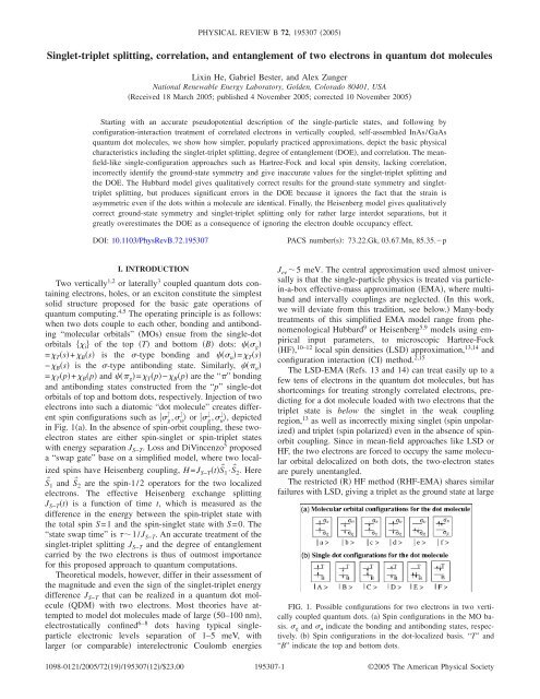
<strong>Singlet</strong>-<strong>triplet</strong> <strong>splitting</strong>, <strong>correlation</strong>, <strong>and</strong> <strong>entanglement</strong> <strong>of</strong> <strong>two</strong> electrons in quantum dot molecules<br />
Lixin He, Gabriel Bester, <strong>and</strong> Alex Zunger<br />
National Renewable Energy Laboratory, Golden, Colorado 80401, USA<br />
Received 18 March 2005; published 4 November 2005; corrected 10 November 2005<br />
Starting with an accurate pseudopotential description <strong>of</strong> the single-particle states, <strong>and</strong> following by<br />
configuration-interaction treatment <strong>of</strong> correlated electrons in vertically coupled, self-assembled InAs/GaAs<br />
quantum dot molecules, we show how simpler, popularly practiced approximations, depict the basic physical<br />
characteristics including the singlet-<strong>triplet</strong> <strong>splitting</strong>, degree <strong>of</strong> <strong>entanglement</strong> DOE, <strong>and</strong> <strong>correlation</strong>. The meanfield-like<br />
single-configuration approaches such as Hartree-Fock <strong>and</strong> local spin density, lacking <strong>correlation</strong>,<br />
incorrectly identify the ground-state symmetry <strong>and</strong> give inaccurate values for the singlet-<strong>triplet</strong> <strong>splitting</strong> <strong>and</strong><br />
the DOE. The Hubbard model gives qualitatively correct results for the ground-state symmetry <strong>and</strong> singlet<strong>triplet</strong><br />
<strong>splitting</strong>, but produces significant errors in the DOE because it ignores the fact that the strain is<br />
asymmetric even if the dots within a molecule are identical. Finally, the Heisenberg model gives qualitatively<br />
correct ground-state symmetry <strong>and</strong> singlet-<strong>triplet</strong> <strong>splitting</strong> only for rather large interdot separations, but it<br />
greatly overestimates the DOE as a consequence <strong>of</strong> ignoring the electron double occupancy effect.<br />
DOI: 10.1103/PhysRevB.72.195307 PACS numbers: 73.22.Gk, 03.67.Mn, 85.35.p<br />
I. INTRODUCTION<br />
Two vertically1,2 or laterally3 coupled quantum dots containing<br />
electrons, holes, or an exciton constitute the simplest<br />
solid structure proposed for the basic gate operations <strong>of</strong><br />
quantum computing. 4,5 The operating principle is as follows:<br />
when <strong>two</strong> dots couple to each other, bonding <strong>and</strong> antibonding<br />
“molecular orbitals” MOs ensue from the single-dot<br />
orbitals i <strong>of</strong> the top T <strong>and</strong> bottom B dots: g =Ts+ Bs is the -type bonding <strong>and</strong> u= Ts<br />
−Bs is the -type antibonding state. Similarly, u =Tp+ Bp <strong>and</strong> g= Tp− Bp are the “” bonding<br />
<strong>and</strong> antibonding states constructed from the “p” single-dot<br />
orbitals <strong>of</strong> top <strong>and</strong> bottom dots, respectively. Injection <strong>of</strong> <strong>two</strong><br />
electrons into such a diatomic “dot molecule” creates differ-<br />
↑ ↑ ↓ ↓<br />
ent spin configurations such as g,u or g,u<br />
, depicted<br />
in Fig. 1a. In the absence <strong>of</strong> spin-orbit coupling, these <strong>two</strong>electron<br />
states are either spin-singlet or spin-<strong>triplet</strong> states<br />
with energy separation JS−T. Loss <strong>and</strong> DiVincenzo5 proposed<br />
a “swap gate” base on a simplified model, where <strong>two</strong> localized<br />
spins have Heisenberg coupling, H=J S−TtS 1·S 2. Here<br />
S 1 <strong>and</strong> S 2 are the spin-1/2 operators for the <strong>two</strong> localized<br />
electrons. The effective Heisenberg exchange <strong>splitting</strong><br />
JS−Tt is a function <strong>of</strong> time t, which is measured as the<br />
difference in the energy between the spin-<strong>triplet</strong> state with<br />
the total spin S=1 <strong>and</strong> the spin-singlet state with S=0. The<br />
“state swap time” is 1/JS−T. An accurate treatment <strong>of</strong> the<br />
singlet-<strong>triplet</strong> <strong>splitting</strong> JS−T <strong>and</strong> the degree <strong>of</strong> <strong>entanglement</strong><br />
carried by the <strong>two</strong> electrons is thus <strong>of</strong> outmost importance<br />
for this proposed approach to quantum computations.<br />
Theoretical models, however, differ in their assessment <strong>of</strong><br />
the magnitude <strong>and</strong> even the sign <strong>of</strong> the singlet-<strong>triplet</strong> energy<br />
difference JS−T that can be realized in a quantum dot molecule<br />
QDM with <strong>two</strong> electrons. Most theories have attempted<br />
to model dot molecules made <strong>of</strong> large 50–100 nm,<br />
electrostatically confined6–8 dots having typical singleparticle<br />
electronic levels separation <strong>of</strong> 1–5 meV, with<br />
larger or comparable interelectronic Coulomb energies<br />
PHYSICAL REVIEW B 72, 195307 2005<br />
J ee5 meV. The central approximation used almost universally<br />
is that the single-particle physics is treated via particlein-a-box<br />
effective-mass approximation EMA, where multib<strong>and</strong><br />
<strong>and</strong> intervally couplings are neglected. In this work,<br />
we will deviate from this tradition, see below. Many-body<br />
treatments <strong>of</strong> this simplified EMA model range from phenomenological<br />
Hubbard 9 or Heisenberg 5,9 models using empirical<br />
input parameters, to microscopic Hartree-Fock<br />
HF, 10–12 local spin densities LSD approximation, 13,14 <strong>and</strong><br />
configuration interaction CI method. 2,15<br />
The LSD-EMA Refs. 13 <strong>and</strong> 14 can treat easily up to a<br />
few tens <strong>of</strong> electrons in the quantum dot molecules, but has<br />
shortcomings for treating strongly correlated electrons, predicting<br />
for a dot molecule loaded with <strong>two</strong> electrons that the<br />
<strong>triplet</strong> state is below the singlet in the weak coupling<br />
region, 13 as well as incorrectly mixing singlet spin unpolarized<br />
<strong>and</strong> <strong>triplet</strong> spin polarized even in the absence <strong>of</strong> spinorbit<br />
coupling. Since in mean-field approaches like LSD or<br />
HF, the <strong>two</strong> electrons are forced to occupy the same molecular<br />
orbital delocalized on both dots, the <strong>two</strong>-electron states<br />
are purely unentangled.<br />
The restricted R HF method RHF-EMA shares similar<br />
failures with LSD, giving a <strong>triplet</strong> as the ground state at large<br />
FIG. 1. Possible configurations for <strong>two</strong> electrons in <strong>two</strong> vertically<br />
coupled quantum dots. a Spin configurations in the MO basis.<br />
g <strong>and</strong> u indicate the bonding <strong>and</strong> antibonding states, respectively.<br />
b Spin configurations in the dot-localized basis. “T” <strong>and</strong><br />
“B” indicate the top <strong>and</strong> bottom dots.<br />
1098-0121/2005/7219/19530712/$23.00 195307-1<br />
©2005 The American Physical Society
HE, BESTER, AND ZUNGER PHYSICAL REVIEW B 72, 195307 2005<br />
interdot separation. The unrestricted U HF Ref. 11 corrects<br />
some <strong>of</strong> the problems <strong>of</strong> RHF by relaxing the requirement<br />
<strong>of</strong> i <strong>two</strong> electrons <strong>of</strong> different spins occupying the<br />
same spatial orbital, <strong>and</strong> ii the single-particle wave functions<br />
have the symmetry <strong>of</strong> the external confining potential.<br />
The UHF-EMA correctly give the singlet lower in energy<br />
than the <strong>triplet</strong>, 12 <strong>and</strong> can also predict Mott localization <strong>of</strong><br />
the electrons in the dot molecule, which breaks the manyparticle<br />
symmetry. 11 However, since in UHF, the symmetrybroken<br />
wave functions are only the eigenstates <strong>of</strong> the z component<br />
<strong>of</strong> total spin S=s 1+s 2, but not <strong>of</strong> S 2 , the UHF-EMA<br />
incorrectly mixes the singlet <strong>and</strong> <strong>triplet</strong>. 11,12 For the simple<br />
case <strong>of</strong> dot molecules having inversion symmetry, e.g., molecules<br />
made <strong>of</strong> spherical dots but not <strong>of</strong> vertical lens-shaped<br />
dots, assuming EMA <strong>and</strong> neglecting spin-orbit coupling,<br />
there is an exact symmetry. For this case, Refs. 16 <strong>and</strong> 17<br />
indeed were able to project out the eigenstates <strong>of</strong> S 2 , yielding<br />
good spin quantum numbers <strong>and</strong> lower energy. However, for<br />
vertically coupled lens shaped quantum dots i.e., realistic<br />
self-assembled systems or even for spherical dots, but in the<br />
presence <strong>of</strong> spin-orbit coupling, there is no exact symmetry.<br />
In this case, configurations with different symmetries may<br />
couple to each other. To get the correct energy spectrum <strong>and</strong><br />
many-body wave functions, a further variation has to be<br />
done after the projection, e.g., using the generalized valence<br />
bond GVB method. 18 For this case <strong>and</strong> other cases a CI<br />
approach is needed.<br />
The CI-EMA has been proven 2,15 to be accurate for treating<br />
few-electron states in large electrostatic dot molecules,<br />
<strong>and</strong> predicts the correct ground state. Finally, recent quantum<br />
Monte Carlo EMA calculations 19 also show that the singlet is<br />
below the <strong>triplet</strong>.<br />
The above discussion pertained to large 50–100 nm<br />
electrostatic-confined dots. Recently, dot molecules have<br />
been fabricated 20,21 from self-assembled InAs/GaAs, <strong>of</strong>fering<br />
a much larger J S−T. Such dots have much smaller confining<br />
dimensions height <strong>of</strong> only 2–5 nm, showing a typical<br />
spacing between electron levels <strong>of</strong> 40–60 meV, smaller interelectronic<br />
Coulomb energies J ee20 meV, <strong>and</strong> exchange<br />
energies <strong>of</strong> K ee3 meV. Such single dots have been accurately<br />
modeled 22 via atomistic pseudopotential theories, applied<br />
to the single-particle problem including multib<strong>and</strong> <strong>and</strong><br />
intervally couplings as well as nonparabolicity, thus completely<br />
avoiding the effective-mass approximation. The<br />
many-particle problem is then described via the all-boundstate<br />
configuration-interaction method. Here we use this<br />
methodology to study the singlet-<strong>triplet</strong> <strong>splitting</strong> in vertically<br />
stacked self-assembled InAs/GaAs dots. We calculate first<br />
the singlet-<strong>triplet</strong> <strong>splitting</strong> vs interdot separation, finding the<br />
singlet to be below the <strong>triplet</strong>. We then simplify our model in<br />
successive steps, reducing the sophistication with which interelectronic<br />
<strong>correlation</strong> is described <strong>and</strong> showing how these<br />
previously practiced approximations 10–14 lead to different<br />
values <strong>of</strong> J S−T, including its sign reversal. This methodology<br />
provides insight into the electronic processes which control<br />
the singlet-<strong>triplet</strong> <strong>splitting</strong> in dot molecules.<br />
The remainder <strong>of</strong> the paper is arranged as follows. In Sec.<br />
II we provide technical details regarding the methodology<br />
we use for the calculations. We then compare the singlet<strong>triplet</strong><br />
<strong>splitting</strong>, degree <strong>of</strong> <strong>entanglement</strong>, <strong>and</strong> <strong>correlation</strong> <strong>of</strong><br />
195307-2<br />
FIG. 2. Geometry <strong>of</strong> the <strong>two</strong> vertically coupled quantum dot<br />
molecule. The interdot distance d is measured from wetting layer to<br />
wetting layer.<br />
<strong>two</strong>-electron states in different levels <strong>of</strong> approximations in<br />
Sec. III. Finally, we summarize in Sec. IV.<br />
II. METHODS<br />
A. Geometry <strong>and</strong> strain relaxation<br />
We consider a realistic dot-molecule geometry4 shown in<br />
Fig. 2, which has recently been used in studying exciton<br />
<strong>entanglement</strong>4,23 <strong>and</strong> <strong>two</strong>-electron states. 24 Each InAs dot is<br />
12 nm wide <strong>and</strong> 2 nm tall, with one monolayer InAs “wetting<br />
layer,” <strong>and</strong> compressively strained by a GaAs matrix.<br />
Even though experimentally grown dot molecules <strong>of</strong>ten have<br />
slightly different size <strong>and</strong> composition pr<strong>of</strong>ile for each dot<br />
within the molecule, here we prefer to consider identical<br />
dots, so as to investigate the extent <strong>of</strong> symmetry breaking<br />
due to many-body effects in the extreme case <strong>of</strong> identical<br />
dots. The minimum-strain configuration is achieved at each<br />
interdot separation d, by relaxing the positions Rn, <strong>of</strong> all<br />
dot+matrix atoms <strong>of</strong> type at site n, so as to minimize the<br />
bond-bending <strong>and</strong> bond-stretching energy using the valence<br />
force field VFF method. 25,26 This shows that both dots have<br />
large <strong>and</strong> nearly constant hydrostatic strain inside the dots<br />
which decays rapidly outside. 24 However, even though the<br />
dots comprising the molecule are geometrically identical, the<br />
strain on the <strong>two</strong> dots is different since the molecule lacks<br />
inversion symmetry. In fact, we found that the top dot is<br />
slightly more strained than the bottom dot. Not surprisingly,<br />
the GaAs region between the <strong>two</strong> dots is more severely<br />
strained than in other parts <strong>of</strong> the matrix, as shown in Fig. 1<br />
<strong>of</strong> Ref. 24 <strong>and</strong> as the <strong>two</strong> dots move apart, the strain between<br />
them decreases.<br />
B. Calculating the single-particle states<br />
The single-particle electronic energy levels <strong>and</strong> wave<br />
functions are obtained by solving the Schrödinger equations<br />
in a pseudopotential scheme,<br />
− 1<br />
2 2 + Vpsrir = iir, 1<br />
where the total electron-ion potential Vpsr is a superposition<br />
<strong>of</strong> local, screened atomic pseudopotentials vr, i.e.,
SINGLE-TRIPLET SPLITTING, CORRELATION, AND… PHYSICAL REVIEW B 72, 195307 2005<br />
V psr= n,v r−R n,. The pseudopotentials used for<br />
InAs/GaAs are identical to those used in Ref. 27 <strong>and</strong> were<br />
tested for different systems. 23,27,28 We ignored spin-orbit coupling<br />
in the InAs/GaAs quantum dots, since it is extremely<br />
small for electrons treated here but not for holes which we<br />
do not discuss in the present work. Without spin-orbit coupling,<br />
the states <strong>of</strong> <strong>two</strong> electrons are either pure singlet or<br />
pure <strong>triplet</strong>. However, if a spin-orbit coupling is introduced,<br />
the singlet state would mix with <strong>triplet</strong> state.<br />
Equation 1 is solved using the “linear combination <strong>of</strong><br />
Bloch b<strong>and</strong>s” LCBB method, 29 where the wave functions<br />
i are exp<strong>and</strong>ed as<br />
<br />
<br />
n,k,J<br />
ir = Cn,k r. 2<br />
n,k<br />
<br />
In the above equation, r are the bulk Bloch<br />
n,k,J<br />
orbitals <strong>of</strong> b<strong>and</strong> index n <strong>and</strong> wave vector k <strong>of</strong> material<br />
=InAs,GaAs, strained uniformly to strain J. The dependence<br />
<strong>of</strong> the basis functions on strain makes them variationally<br />
efficient. Note that the potential Vpsr itself also has<br />
the inhomogeneous strain dependence through the atomic<br />
position Rn,. We use for the basis set J=0 for the unstrained<br />
GaAs matrix material, <strong>and</strong> an average J value from<br />
VFF for the strained dot material InAs. For the InAs/GaAs<br />
system, we use n=2 including spin for electron states on a<br />
6628 k mesh. A single dot with the geometry <strong>of</strong> Fig. 2<br />
base=12 nm <strong>and</strong> height=2 nm has three bound electron<br />
states s, p1, <strong>and</strong> p2 <strong>and</strong> more than ten bound hole states.<br />
The lowest exciton transition in the single dot occurs at energy<br />
1.09 eV. For the dot molecule the resulting singleparticle<br />
states are, in order <strong>of</strong> increasing energy, g <strong>and</strong> u bonding <strong>and</strong> antibonding combination <strong>of</strong> the s-like singledot<br />
orbitals, <strong>and</strong> the doubly nearly degenerate u <strong>and</strong> g, originating from doubly nearly degenerate “p” orbitals<br />
split by a few meV in a single dot. Here, we use the symbols<br />
g <strong>and</strong> u to denote symmetric <strong>and</strong> antisymmetric states,<br />
even though in our case the single-particle wave functions<br />
are actually asymmetric. 24 We define the difference between<br />
the respective dot molecule eigenvalues as = u<br />
− g <strong>and</strong> = g− u.<br />
C. Calculating the many-particle states<br />
The Hamiltonian <strong>of</strong> interacting electrons can be written as<br />
†<br />
H = iii +<br />
i<br />
1<br />
2 ij † †<br />
klij k<br />
ijkl ,<br />
l, 3<br />
where i= u, g, u, g are the single-particle energy levels<br />
<strong>of</strong> the ith molecular orbital, while , =1, 2 are spin indi-<br />
ij<br />
ces. The kl are the Coulomb integrals between molecular<br />
orbitals i, j, k, <strong>and</strong> l, ij<br />
kl =dr dr * *<br />
i rj rkr lr<br />
. 4<br />
r − rr − r<br />
ij ij<br />
The Jij= ji <strong>and</strong> Kij= ij are diagonal Coulomb <strong>and</strong> exchange<br />
integrals, respectively. The remaining terms are called <strong>of</strong>fdiagonal<br />
or scattering terms. All Coulomb integrals are cal-<br />
195307-3<br />
culated numerically from atomistic wave functions. 30 We use<br />
a phenomenological, position-dependent dielectric function<br />
r−r to screen the electron-electron interaction. 30<br />
We solve the many-body problem <strong>of</strong> Eq. 3 via the CI<br />
method, by exp<strong>and</strong>ing the N-electron wave function in a set<br />
† † †<br />
<strong>of</strong> Slater determinants, e1 ,e2 ,…,e =<br />
N e1e2<br />
¯eN0,<br />
†<br />
where ei creates an electron in the state ei. The th manyparticle<br />
wave function is then the linear combinations <strong>of</strong> the<br />
determinants,<br />
= Ae1,e 2,…,e Ne1 ,e2 ,…,e . 5<br />
N<br />
e1 ,e2 ,…,eN In this paper, we only discuss the <strong>two</strong>-electron problem, i.e.,<br />
N=2. Our calculations include all possible Slater determinants<br />
for the six single-particle levels.<br />
D. Calculating pair-<strong>correlation</strong> functions <strong>and</strong> degree<br />
<strong>of</strong> <strong>entanglement</strong><br />
We calculate in addition to the energy spectrum <strong>and</strong> the<br />
singlet-<strong>triplet</strong> <strong>splitting</strong> JS−T also the pair-<strong>correlation</strong> functions<br />
<strong>and</strong> the degrees <strong>of</strong> <strong>entanglement</strong> DOE. The pair-<strong>correlation</strong><br />
function Pr,r for an N-particle system is defined as the<br />
probability <strong>of</strong> finding an electron at r, given that the other<br />
electron is at r, i.e.,<br />
P r,r = dr 3 ¯ dr N r,r,r 3,…,r N 2 , 6<br />
where, r 1,…,r N is the N-particle wave function <strong>of</strong> state<br />
. For <strong>two</strong> electrons, the pair-<strong>correlation</strong> function is just<br />
P r,r= r,r 2 .<br />
The degree <strong>of</strong> <strong>entanglement</strong> DOE is one <strong>of</strong> the most<br />
important quantities for successful quantum gate operations.<br />
For distinguishable particles such as electron <strong>and</strong> hole, the<br />
DOE can be calculated from von Neumann–entropy<br />
formulation. 31–34 However, for indistinguishable particles,<br />
there are some subtleties 35–41 for defining the DOE since it is<br />
impossible to separate the <strong>two</strong> identical particles. Recently, a<br />
quantum <strong>correlation</strong> function 35 has been proposed for indistinguishable<br />
particles using the Slater decompositions. 42 We<br />
adapt this quantum <strong>correlation</strong> function to define the DOE<br />
for indistinguishable fermions as<br />
S =− u<br />
2 2<br />
zi log2 zi , 7<br />
where z i are Slater decomposition coefficients. The details <strong>of</strong><br />
deriving Eq. 7 are given in Appendix A. We also show in<br />
Appendix A that the DOE measure <strong>of</strong> Eq. 7 reduces to the<br />
usual von Neumann–entropy formulation when the <strong>two</strong> electrons<br />
are far from each other.<br />
III. RESULTS<br />
Figure 3 shows the bonding-antibonding <strong>splitting</strong> d<br />
between the molecular orbitals vs interdot separation d measured<br />
from one wetting layer to the other, showing also the<br />
value sp= p− s <strong>of</strong> the <strong>splitting</strong> between the p <strong>and</strong> s orbital<br />
energies <strong>of</strong> a single dot i.e., d→. The bonding-
HE, BESTER, AND ZUNGER PHYSICAL REVIEW B 72, 195307 2005<br />
FIG. 3. The bonding-antibonding <strong>splitting</strong> = g− u<br />
solid line <strong>and</strong> singlet-<strong>triplet</strong> <strong>splitting</strong> JS−T=E 3 −E 1 a<br />
g <br />
dashed line vs interdot distance d. We also show the single-dot s,<br />
p orbitals <strong>splitting</strong> sp=e s−e p <strong>and</strong> the s orbital Coulomb interaction<br />
JC. We define “strong coupling” by sp4 nm<strong>and</strong> “weak<br />
coupling,” sp5 nm.<br />
antibonding <strong>splitting</strong> decays approximately exponentially as<br />
=2.87 exp−d/1.15 eV between d4 <strong>and</strong> 8 nm. The result<br />
<strong>of</strong> bonding-antibonding <strong>splitting</strong> includes <strong>two</strong> competing<br />
effects. On one h<strong>and</strong>, large interdot distance d reduces the<br />
coupling between the <strong>two</strong> dots; on the other h<strong>and</strong>, the strain<br />
between the dots is also reduced, leading to a lower tunneling<br />
barrier, thus increasing coupling. The local maximum <strong>of</strong><br />
at d=8.5 nm is a consequence <strong>of</strong> the this competition.<br />
Recent experiments 20,21 show the bonding-antibonding <strong>splitting</strong><br />
<strong>of</strong> about 4 meV at d=11.5 nm for vertically coupled<br />
InAs/GaAs quantum dot molecules, <strong>of</strong> similar magnitude as<br />
the value obtained here 1 meV, considering that the measured<br />
dot molecule is larger height/base=4 nm/40 nm<br />
rather than 2 nm/12nm in our calculations <strong>and</strong> possibly<br />
asymmetric. We also give in Fig. 3 the interelectronic Coulomb<br />
energy J C <strong>of</strong> a single-dot s orbital. We define the<br />
strong-coupling region as sp, <strong>and</strong> the weak-coupling<br />
region sp. We see in Fig. 3 strong coupling for d4<br />
nm, <strong>and</strong> weak coupling for d5 nm. In the weak-coupling<br />
region, the levels are well above the levels. We also<br />
define “strong confinement” as spJ C, <strong>and</strong> weak confinement<br />
as the reverse inequality. Figure 3 shows that our dot is<br />
FIG. 4. Selected Coulomb integrals for molecular orbitals. J gg is<br />
the self-Coulomb energy <strong>of</strong> the g orbital <strong>and</strong> J gu is the Coulomb<br />
energy between g <strong>and</strong> u orbitals, while K gu is the exchange energy<br />
between g <strong>and</strong> u orbitals.<br />
195307-4<br />
FIG. 5. Color online a Two-electron states calculated from<br />
CI using all confined MO from LCBB level 1, including the singlet<br />
1 a 1<br />
g , u, 1 b<br />
g states <strong>and</strong> the threefold degenerated <strong>triplet</strong><br />
states 3 u as well as <strong>two</strong> threefold degenerated <strong>triplet</strong> states 3 u .<br />
b Two electron states calculated from the single-configuration approximation<br />
level 3. c Comparison <strong>of</strong> the singlet-<strong>triplet</strong> <strong>splitting</strong><br />
calculated from level-1, -3, <strong>and</strong> -4 theories.<br />
in the strong-confinement regime. In contrast, electrostatic<br />
dots 6–8 are in the weak confinement regime.<br />
We next discuss the <strong>two</strong>-electron states in the QDMs <strong>and</strong><br />
examine several different approximations which we call levels<br />
1–4, by comparing the properties <strong>of</strong> the ground states, the<br />
singlet-<strong>triplet</strong> energy separation J S−T <strong>and</strong> the pair-<strong>correlation</strong><br />
functions as well as the degree <strong>of</strong> <strong>entanglement</strong> for each<br />
state. Starting from our most complete model level 1 <strong>and</strong><br />
simplifying it in successive steps, we reduce the sophistication<br />
with which interelectronic <strong>correlation</strong> is described <strong>and</strong><br />
show how these previously practiced approximations lead to<br />
different values <strong>of</strong> J S−T including its sign reversal, <strong>and</strong> different<br />
degree <strong>of</strong> <strong>entanglement</strong>. This methodology provides<br />
insight into the electronic features which control singlet<strong>triplet</strong><br />
<strong>splitting</strong> <strong>and</strong> electron-electron <strong>entanglement</strong> in dot<br />
molecules.
SINGLE-TRIPLET SPLITTING, CORRELATION, AND… PHYSICAL REVIEW B 72, 195307 2005<br />
FIG. 6. Isospin, defined as the difference in the number <strong>of</strong> electrons<br />
occupying the bonding NB <strong>and</strong> antibonding NAB states, <strong>of</strong><br />
the 1 a<br />
g state in level-1 <strong>and</strong> level-3 theories.<br />
A. Level-1 theory: All-bound-state configuration interaction<br />
We first study the <strong>two</strong>-electron states by solving the CI<br />
Eq. 5, using all confined molecular orbitals g, u <strong>and</strong> g,<br />
u, to construct the Slater determinants. This gives a total <strong>of</strong><br />
66 Slater determinants. The continuum states are far above<br />
the bound state, <strong>and</strong> are thus not included in the CI basis.<br />
Figure 4 shows some important matrix elements, including<br />
J gg Coulomb energy <strong>of</strong> g MO, J gu Coulomb energy between<br />
g <strong>and</strong> u, <strong>and</strong> K gu exchange energy between g <strong>and</strong><br />
u. The Coulomb energy between u MO, J uu is nearly<br />
identical to J gg <strong>and</strong> therefore is not plotted. Diagonalizing the<br />
all-bound-state CI problem gives the <strong>two</strong>-particle states,<br />
shown in Fig. 5a. We show all six states where both<br />
electrons occupy the states <strong>and</strong> the <strong>two</strong> lowest threefold<br />
degenerate 3 u states where one electron occupies the g<br />
<strong>and</strong> one occupies one <strong>of</strong> the levels. We observe that:<br />
i The ground state is singlet 1 a<br />
g for all dot-dot distances.<br />
However, the character <strong>of</strong> the state is very different at<br />
different interdot separation d, which can be analyzed by the<br />
isospin <strong>of</strong> the state, 43 defined as the difference in the number<br />
<strong>of</strong> electrons occupying the bonding NB <strong>and</strong> antibonding<br />
NAB states in a given CI state, i.e., Iz=N B−N AB/2, where<br />
NB <strong>and</strong> NAB are obtained from Eq. 5. As shown in Fig. 6,<br />
Izd <strong>of</strong> the 1 a<br />
g state is very different at different interdot<br />
distances: At small interdot distance, the dominant configu-<br />
↑ ↓<br />
ration <strong>of</strong> the ground state is g,g both electrons occupy<br />
bonding state <strong>and</strong> NB=2, <strong>and</strong> Iz1. However, in the weak-<br />
coupling region, there is significant mixing <strong>of</strong> bonding g <strong>and</strong> antibonding states u, <strong>and</strong> Iz is smaller than 1, e.g.,<br />
Iz0.2 at d=9.5 nm. At infinite separation, where the bonding<br />
<strong>and</strong> antibonding states are degenerate, one expects<br />
Iz→ 0.<br />
ii Next to the ground state, we find in Fig. 5a the<br />
threefold degenerate <strong>triplet</strong> states 3 u, with Sz=1, −1, <strong>and</strong> 0.<br />
In the absence <strong>of</strong> spin-orbit coupling, <strong>triplet</strong> states will not<br />
couple to singlet states. If we include spin-orbit coupling, the<br />
<strong>triplet</strong> may mix with the singlet state, <strong>and</strong> the degeneracy<br />
will be lifted. At large interdot distances, the ground-state<br />
singlet 1 a 3<br />
g <strong>and</strong> <strong>triplet</strong> states u are degenerate. The split-<br />
ting <strong>of</strong> total CI energy between ground-state singlet <strong>and</strong> <strong>triplet</strong><br />
JS−T=E 3 −E 1 g is plotted in Fig. 3 on a logarithmic<br />
scale. As we can see, JS−T also decays approximately exponentially<br />
between 4 <strong>and</strong> 8 nm, <strong>and</strong> can be fitted as<br />
JS−T=5.28 exp−d/0.965eV. The decay length <strong>of</strong> 0.965 nm<br />
is shorter than the decay length 1.15 nm <strong>of</strong> . At small<br />
interdot separations, JS−T in Fig. 3, as expected from a<br />
simple Heitler-London model. 9<br />
iii The <strong>two</strong> excited singlet states originating from the<br />
occupation <strong>of</strong> u antibonding states, 1 u <strong>and</strong> 1 g<br />
b are further<br />
above the 3 u state.<br />
iv The lowest 3 u states are all <strong>triplet</strong> states. They are<br />
energetically very close to each other since we have <strong>two</strong><br />
nearly degenerate u MO states. In the weak-coupling region,<br />
the u states are well above the states, as a<br />
consequence <strong>of</strong> large single-particle energy difference<br />
u− u. However, the u, <strong>and</strong> 1 g<br />
b cross at about 4.5<br />
nm, where the single-particle MO level u is still much<br />
higher than u. In this case, the Coulomb <strong>correlation</strong>s have to<br />
be taken into account.<br />
In the following sections, we enquire as to possible, popularly<br />
practiced simplifications over the all-bound-states CI<br />
treatment.<br />
B. Level-2 theory: Reduced CI in the molecular basis<br />
In level-2 theory, we will reduce the full 6666 CI problem<br />
<strong>of</strong> level 1 to one that includes only the g <strong>and</strong> u basis,<br />
giving a 66 CI problem. The six many-body basis<br />
↑ ↑ ↓ ↓<br />
states are shown in Fig. 1a, a= g,u<br />
, b=g ,u,<br />
↑<br />
c= g,u<br />
↓ , d=g<br />
↓ ,u<br />
↑ , e=g<br />
↑ ,g<br />
↓ , f=u<br />
↑ ,u<br />
↓ . In this<br />
basis set, the CI problem is reduced to a 66 matrix eigenvalue<br />
equation,<br />
g + u + Jgu − Kgu 0 0 0 0 0<br />
0 g + u + Jgu − Kgu 0 0 0 0<br />
gu<br />
gu<br />
0 0 g + u + Jgu − Kgu − gg − uu H =<br />
gu<br />
gu<br />
8<br />
0 0 − Kgu g + u + Jgu gg uu gg<br />
gg<br />
gg<br />
0 0 − gu gu 2g + Jgg uu uu<br />
uu<br />
uu<br />
0 0 − gu gu gg 2u + Juu, 195307-5
HE, BESTER, AND ZUNGER PHYSICAL REVIEW B 72, 195307 2005<br />
where g <strong>and</strong> u are the single-particle energy levels for the<br />
MOs g <strong>and</strong> u, respectively. In the absence <strong>of</strong> spin-orbit<br />
coupling, the <strong>triplet</strong> states a <strong>and</strong> b are not coupled to any<br />
other states, as required by the total spin conservation, <strong>and</strong><br />
thus they are already eigenstates. The rest <strong>of</strong> the matrix can<br />
be solved using the integrals calculated from Eq. 4. The<br />
results <strong>of</strong> the 66 problem were compared not shown to<br />
the all-bound-state CI results: We find that the states <strong>of</strong><br />
level-2 theory are very close to those <strong>of</strong> the all-bound-state<br />
CI calculations, indicating a small coupling between <strong>and</strong> <br />
orbitals in the strong confinement region. We thus do not<br />
show graphically the results <strong>of</strong> level 2. However, since we<br />
use only orbitals, the states <strong>of</strong> level 1 Fig. 5a are<br />
absent in level-2 theory. Especially, the important feature <strong>of</strong><br />
crossover between <strong>and</strong> u states at 4 <strong>and</strong> 4.5 nm is missing.<br />
C. Level-3 theory: Single-configuration in the molecular basis<br />
As is well known, mean-field-like treatments such as RHF<br />
<strong>and</strong> LSD usually give incorrect dissociation behavior <strong>of</strong> molecules,<br />
as the <strong>correlation</strong> effects are not adequately treated.<br />
Given that RHF <strong>and</strong> LSD are widely used in studying<br />
QMDs, 10,13,14 it is important to underst<strong>and</strong> under which circumstance<br />
the methods will succeed <strong>and</strong> under which circumstance<br />
they will fail in describing the few-electron states<br />
in a QDM. In level-3 theory, we thus mimic the mean-field<br />
theory by further ignoring the <strong>of</strong>f-diagonal Coulomb inte-<br />
gu gu<br />
grals in Eq. 8 <strong>of</strong> level-2 theory, i.e., we assume uu=gg uu<br />
=gg=0. This approximation is equivalent to ignoring the<br />
coupling between different configurations, <strong>and</strong> is thus called<br />
“single-configuration” SC approximation. At the SC level,<br />
we have very simple analytical solutions <strong>of</strong> the <strong>two</strong>-electron<br />
states,<br />
E1 a<br />
g =2g + Jgg; 1 a<br />
g = e, 9<br />
E 3 u = g + u + J gu − K gu;<br />
<br />
3<br />
+ u = a,<br />
3<br />
−u = b,<br />
3<br />
0u = c − d,<br />
10<br />
E 1 u = g + u + J gu + K gu; 1 u = c + d, 11<br />
E1 b<br />
g =2u + Juu; 1 b<br />
g = f. 12<br />
The energies are plotted in Fig. 5b. When comparing the <br />
states <strong>of</strong> the SC approach to the all-bound-state CI results in<br />
Fig. 5a, we find good agreement in the strong-coupling<br />
region for d5 nmsee Fig. 3. However, the SC approximation<br />
fails qualitatively at larger inter-dot separations in<br />
<strong>two</strong> aspects: i The order <strong>of</strong> singlet state 1 a<br />
g <strong>and</strong> <strong>triplet</strong><br />
state 3 u is reversed see Figs. 5b <strong>and</strong> 5c. ii The 1 a<br />
g <strong>and</strong> 3 u states fail to be degenerate at large interdot separation.<br />
This lack <strong>of</strong> degeneracy is also observed for 1 b<br />
g <strong>and</strong><br />
1 u. These failures are due to the absence <strong>of</strong> <strong>correlation</strong>s in<br />
the SC approximation. Indeed as shown in Fig. 6, the accurate<br />
level-1 ground-state singlet has considerable mixing <strong>of</strong><br />
195307-6<br />
antibonding states, i.e., Iz→0 at large d. However, in the SC<br />
approximation both electrons are forced to occupy the g orbital in the lowest singlet state 1 a<br />
g as a consequence <strong>of</strong><br />
the lack <strong>of</strong> the coupling between the configuration e <strong>of</strong> Fig.<br />
1a <strong>and</strong> other configurations. As a result, in level-3 theory,<br />
the isospins are forced to be Iz=1 for 1 a<br />
g at all interdot<br />
distances d, which pushes the singlet energy higher than the<br />
<strong>triplet</strong>.<br />
D. Level-4 theory: Hubbard model <strong>and</strong> Heisenberg model<br />
in a dot-centered basis<br />
The Hubbard model <strong>and</strong> the Heisenberg model are <strong>of</strong>ten<br />
used5 to analyze <strong>entanglement</strong> <strong>and</strong> gate operations for <strong>two</strong><br />
spins qubits in a QDM. Here, we analyze the extent to which<br />
such approaches can correctly capture the qualitative physics<br />
given by more sophisticated models. Furthermore, by doing<br />
so, we obtain the parameters <strong>of</strong> the models from realistic<br />
calculations.<br />
1. Transforming the states to a dot-centered basis<br />
Unlike the level-1–3 theories, the Hubbard <strong>and</strong> the<br />
Heisenberg models are written in a dot-centered basis as<br />
shown in Fig. 1b, rather than in the molecular basis <strong>of</strong> Fig.<br />
1a. In a dot-centered basis, the Hamiltonian <strong>of</strong> Eq. 3 can<br />
be rewritten as<br />
†<br />
H = e11 + t<br />
2<br />
1 <br />
2 1 ,2<br />
<br />
1 ,2 <br />
+ 1<br />
2 <br />
1 ,…, 4<br />
<br />
,<br />
<br />
˜ 1 ,21 † †<br />
3 ,4 ,2<br />
,<br />
3 , 4 ,, 13<br />
†<br />
where =l, p <strong>and</strong> , creates an electron in the<br />
l=s, p,… orbital on the p=T,B dot with spin that has<br />
single-particle energy e. Here, t1 is the coupling between<br />
2<br />
the 1 <strong>and</strong> 2 orbitals, <strong>and</strong> ˜ 1,2 3 , is the Coulomb integral <strong>of</strong><br />
4<br />
single-dot orbitals 1 , 2 , 3 , <strong>and</strong> 4 .<br />
We wish to construct a Hubbard Hamiltonian whose parameters<br />
are taken from the fully atomistic single-particle<br />
theory. To obtain such parameters in Eq. 13 including<br />
e, t1 , <strong>and</strong> <br />
2 ˜ 1,2, 3 , we resort to a Wannier-like transforma-<br />
4<br />
tion, which transform the “molecular” orbitals Fig. 1a<br />
into single-dot “atomic” orbitals Fig. 1b. The latter dotcentered<br />
orbitals are obtained from a unitary rotation <strong>of</strong> the<br />
molecular orbitals i, i.e.,<br />
= U,ii, 14<br />
i=1<br />
where i is the ith molecular orbitals, is the single dotcentered<br />
orbitals, <strong>and</strong> U are unitary matrices, i.e., U † U=I.We<br />
chose the unitary matrices that maximize the total orbital<br />
self-Coulomb energy. The procedure <strong>of</strong> finding these unitary<br />
matrices is described in detail in Appendix B. The dotcentered<br />
orbitals constructed this way are approximately invariant<br />
to the change <strong>of</strong> coupling between the dots. 44 Once<br />
we have the U matrices, we can obtain all the parameters in<br />
Eq. 13 by transforming them from the molecular basis. The
SINGLE-TRIPLET SPLITTING, CORRELATION, AND… PHYSICAL REVIEW B 72, 195307 2005<br />
FIG. 7. a Effective single-particle energy levels <strong>of</strong> s orbitals<br />
localized on the top e T <strong>and</strong> bottom e B dots. b Intradot Coulomb<br />
energy J TT, J BB, interdot Coulomb energy J TB <strong>and</strong> interdot exchange<br />
energy K TB magnified by a factor 100. The dashed line<br />
gives the single-dot s orbital self-Coulomb energy J C.<br />
Coulomb integrals in the new basis set are given by Eq. B2,<br />
while other quantities including the effective single-particle<br />
levels e for the th dot-centered orbital, <strong>and</strong> the coupling<br />
between the 1th <strong>and</strong> 2th orbitals t 1 2 can be obtained from<br />
e = T ˆ = i<br />
t 1 2 = 1 T ˆ 2 = i<br />
*<br />
U,iU,i i, 15<br />
*<br />
U1 ,iU2<br />
,ii, 16<br />
where i is the single-particle level <strong>of</strong> the ith molecular orbital,<br />
<strong>and</strong> T ˆ is kinetic energy operator. Using the transformation<br />
<strong>of</strong> Eq. 15, Eq. 16, <strong>and</strong> Eq. B2, we calculate all<br />
parameters <strong>of</strong> Eq. 13. Figure 7a shows the effective<br />
single-dot energy <strong>of</strong> the “s” orbitals obtained in the Wannier<br />
representation for both top <strong>and</strong> bottom dots. We see that the<br />
effective single-dot energy levels increase rapidly for small<br />
d. Furthermore, the energy levels for the top <strong>and</strong> bottom<br />
orbitals are split due to the strain asymmetry between the<br />
<strong>two</strong> dots. We compute the Coulomb energies J TT, J BB <strong>of</strong> the<br />
“s” orbitals on both top <strong>and</strong> bottom dots, <strong>and</strong> the interdot<br />
Coulomb <strong>and</strong> exchange energies J TB <strong>and</strong> K TB <strong>and</strong> plot these<br />
quantities in Fig. 7b. Since J TT <strong>and</strong> J BB are very similar, we<br />
plot only J TT. As we can see, the Coulomb energies <strong>of</strong> the<br />
dot-centered orbitals are very close to the Coulomb energy <strong>of</strong><br />
the s orbitals <strong>of</strong> an isolated single dot dashed line. The<br />
interdot Coulomb energy J TB has comparable amplitude to<br />
J TT <strong>and</strong> decays slowly with distance, <strong>and</strong> remain very significant,<br />
even at large separations. However, the exchange<br />
energy between the orbitals localized on the top <strong>and</strong> bottom<br />
dot K TB is extremely small even when the dots are very<br />
close.<br />
2. “First-principles” Hubbard model <strong>and</strong> Heisenberg model:<br />
Level 4<br />
In level-4 approximation, we use only the “s” orbital in<br />
each dot. Figure 1b shows all possible many-body basis<br />
functions <strong>of</strong> <strong>two</strong> electrons, where the top <strong>and</strong> bottom dots are<br />
denoted by “T” <strong>and</strong> “B,” respectively. The Hamiltonian in<br />
this basis set is<br />
T + eB + JTB − KTB 0 0 0 0 0<br />
0 eT + eB + JTB − KTB 0 0 0 0<br />
0 0 eT + eB + JTB − KTB t − ˜ TB<br />
BB t − <br />
H =e ˜ TT<br />
TB<br />
0 0 − KTB eT + eB + JTB − t + ˜ TB<br />
BB − t + ˜ TB<br />
TT 0 0 t − ˜ TB<br />
BB<br />
− t + ˜ TB<br />
BB 2eB + JBB 0<br />
0 0 t − ˜ TB<br />
TT<br />
− t + ˜ TB<br />
TT 17<br />
0 2eT + JTT, where t=t TB <strong>and</strong> to simplify the notation, we ignore the orbital<br />
index “s.” If we keep all the matrix elements, the description<br />
using the molecular basis <strong>of</strong> Fig. 1a <strong>and</strong> the dot<br />
localized basis <strong>of</strong> Fig. 1b are equivalent, since they are<br />
connected by unitary transformations. We now simplify Eq.<br />
17 by ignoring the <strong>of</strong>f-diagonal Coulomb integrals. The<br />
195307-7<br />
resulting Hamiltonian is the single-b<strong>and</strong> Hubbard model.<br />
Unlike level-3 theory, in this case, ignoring <strong>of</strong>f-diagonal<br />
Coulomb integrals but keeping hopping can still give qualitatively<br />
correct results, due to the fact that <strong>of</strong>f-diagonal Coulomb<br />
integrals such as ˜ TB<br />
BB t, <strong>and</strong> the <strong>correlation</strong> is mainly<br />
carried by interdot hopping t. We can further simplify the
HE, BESTER, AND ZUNGER PHYSICAL REVIEW B 72, 195307 2005<br />
model by assuming eT=e B=; JTT=J BB=U; <strong>and</strong> let JTB=V, KTB=K. We can then solve the simplified eigenvalue equation<br />
analytically. The eigenvalues <strong>of</strong> the above Hamiltonian<br />
are in order <strong>of</strong> increasing energy:<br />
i ground-state singlet 1 a<br />
g ,<br />
E =2 + 1<br />
2 U + V + K − 16t2 + U − V − K2; 18<br />
ii <strong>triplet</strong> states threefold degenerate 3 u, iii singlet 1 u,<br />
iv singlet 1 b<br />
g ,<br />
E =2 + V − K; 19<br />
E =2 + U; 20<br />
E =2 + 1<br />
2 U + V + K + 16t2 + U − V − K2. 21<br />
In the Hubbard limit where Coulomb energy Ut, the<br />
singlet-<strong>triplet</strong> <strong>splitting</strong> JS−T=E 3 −E 1 g4t2 /U−V,<br />
which reduces the model to the Heisenberg model<br />
H = 4t2<br />
U − V S T · S B, 22<br />
where S T <strong>and</strong> S B are the spin vectors on the top <strong>and</strong> bottom<br />
dots. The Heisenberg model gives the correct order for<br />
singlet <strong>and</strong> <strong>triplet</strong> states. The singlet-<strong>triplet</strong> <strong>splitting</strong><br />
J S−T=4t 2 /U−V is plotted in Fig. 5c <strong>and</strong> compared to the<br />
results from all-bound-state CI calculations level 1, <strong>and</strong><br />
single-configuration approximations level 3. As we can see,<br />
at d6.5 nm, the agreement between the Heisenberg model<br />
with CI is good, but the Heisenberg model greatly overestimates<br />
J S−T at d6 nm.<br />
E. Comparison <strong>of</strong> pair-<strong>correlation</strong> functions<br />
for level-1 to 4 theories<br />
In the previous sections, we compared the energy levels<br />
<strong>of</strong> <strong>two</strong>-electron states in several levels <strong>of</strong> approximations to<br />
all-bound-state CI results level 1. We now provide further<br />
comparison <strong>of</strong> level-1–4 theories by analyzing the pair<strong>correlation</strong><br />
functions <strong>and</strong> calculating the electron-electron<br />
<strong>entanglement</strong> at different levels <strong>of</strong> approximations.<br />
In Fig. 8 we show the pair-<strong>correlation</strong> functions <strong>of</strong> Eq. 6<br />
for the 1 a 1<br />
g <strong>and</strong> g<br />
b states at d7 nm for level-1 <strong>and</strong><br />
level-3 theories. The <strong>correlation</strong> functions give the probability<br />
<strong>of</strong> finding the second electron when the first electron is<br />
fixed at the position shown by the arrows at the center <strong>of</strong> the<br />
bottom dot left-h<strong>and</strong> side <strong>of</strong> Fig. 8 or the top dot righth<strong>and</strong><br />
side <strong>of</strong> Fig. 8. Level-1 <strong>and</strong> level-2 theories give<br />
<strong>correlation</strong>-induced electron localization at large d: for the<br />
1 g<br />
a state, the <strong>two</strong> electrons are localized on different dots,<br />
while for the 1 b<br />
g state, both electrons are localized on the<br />
same dot. 24 In contrast, level-3 theory shows delocalized<br />
states because <strong>of</strong> the lack <strong>of</strong> configuration mixing. This problem<br />
is shared by RHF <strong>and</strong> LSD approximations.<br />
195307-8<br />
FIG. 8. Color online Comparison <strong>of</strong> pair-<strong>correlation</strong> functions<br />
calculated from a level-1 <strong>and</strong> b level-3 theory for the 1 a<br />
g state<br />
<strong>and</strong> c level-1 <strong>and</strong> d level-3 theory for the 1 b<br />
g state at<br />
d7 nm. On the left-h<strong>and</strong> side, the first electron is fixed at the<br />
center <strong>of</strong> the bottom dot, while on the right-h<strong>and</strong> side, the first<br />
electon is fixed at the center <strong>of</strong> the top dot, as indicated by the<br />
arrows.<br />
F. Comparison <strong>of</strong> the degree <strong>of</strong> <strong>entanglement</strong><br />
for levels-1 to 4 theories<br />
The DOE <strong>of</strong> the four “” states are plotted in Fig. 9 for<br />
level-1, level-3, <strong>and</strong> level-4 theories; the DOEs <strong>of</strong> level-2<br />
theory are virtually identical to those <strong>of</strong> level-1 theory, <strong>and</strong><br />
are therefore not plotted. We see that the Hubbard model has<br />
generally reasonable agreement with level-1 theory while the<br />
DOEs calculated from level-3 <strong>and</strong> level-4 Heisenberg<br />
model theories deviate significantly from the level-1 theory,<br />
which is addressed below.<br />
i The 1 a<br />
g state: The level-1 theory Fig. 9a, shows<br />
that the DOE <strong>of</strong> 1 g<br />
a increases with d <strong>and</strong> approaches 1 at<br />
large d. The Hubbard model <strong>of</strong> level-4 theory Fig. 9c<br />
gives qualitatively correct DOE for this state except for some<br />
details. However, level-3 theory Fig. 9b gives DOE<br />
S=0 because the wave function <strong>of</strong> 1 a<br />
g is a single Slater<br />
determinant e see Eq. 9. For the same reason, the DOEs
SINGLE-TRIPLET SPLITTING, CORRELATION, AND… PHYSICAL REVIEW B 72, 195307 2005<br />
FIG. 9. Color online Comparison <strong>of</strong> the DOE calculated from<br />
a level-1, b level-3, <strong>and</strong> c level-4 theories for <strong>two</strong>-electron<br />
states. In panel c, both the DOE <strong>of</strong> the Hubbard model solid<br />
lines <strong>and</strong> <strong>of</strong> the Heisenberg model for 1 a<br />
g state dashed line are<br />
shown.<br />
<strong>of</strong> the 1 a<br />
g state in RHF <strong>and</strong> LSD approximations are also<br />
zero as a consequence <strong>of</strong> lack <strong>of</strong> <strong>correlation</strong>. In contrast, the<br />
Heisenberg model <strong>of</strong> level-4 theory gives S 1 a<br />
g =1. This is<br />
because the Heisenberg model assumes that the both electrons<br />
are localized on different dots with zero double occupancy,<br />
<strong>and</strong> thus overestimates the DOE. 24,45<br />
ii The 1 b<br />
g state: The Hubbard model gives the DOE <strong>of</strong><br />
the 1 b 1 a<br />
g state identical to that <strong>of</strong> g state. This is different<br />
from the result <strong>of</strong> level-1 theory, especially at large inter-dot<br />
separations. The difference comes from the assumption in the<br />
Hubbard model that the energy levels <strong>and</strong> wave functions on<br />
the top dot <strong>and</strong> on the bottom dot are identical while as<br />
discussed in Ref. 24, the wave functions are actually asymmetric<br />
due to inhomogeneous strain in the real system. At<br />
d8 nm, the 1 b<br />
g state is the supposition <strong>of</strong> E <strong>and</strong> F<br />
configurations in the Hubbard model leading to S=1, while<br />
195307-9<br />
in level-1 theory, the <strong>two</strong> electrons are both localized on the<br />
top dots F at d9 nm, 24 resulting in near zero <strong>entanglement</strong>.<br />
For the same reason discussed in i, the level-3 theory<br />
gives S 1 g<br />
b =0.<br />
iii The 1 u state: Both the level-3 theory <strong>and</strong> Hubbard<br />
model give S 1 u=1. However, the S 1 u <strong>of</strong> the level-1<br />
theory has more features as the consequence <strong>of</strong> the asymme-<br />
try <strong>of</strong> the system. In contrast to the 1 b 1<br />
g state, in the u<br />
state, both electrons are localized on the bottom dot leading<br />
to near zero <strong>entanglement</strong> at d9 nm.<br />
iv The 3 u state: All levels <strong>of</strong> theories give very close<br />
3<br />
results <strong>of</strong> DOE for the 0u state. Actually, in level-1 theory,<br />
3<br />
the DOE <strong>of</strong> the 0u state is only slightly larger than 1, indicating<br />
weak <strong>entanglement</strong> <strong>of</strong> the <strong>and</strong> orbitals the maximum<br />
<strong>entanglement</strong> one can get from the total <strong>of</strong> six orbitals<br />
is Smax=log26, while in all other theories including the<br />
level-2 theory they are exactly 1 since these theories include<br />
only <strong>two</strong> orbitals. The small coupling between <strong>and</strong> <br />
orbitals is desirable for quantum computation, which requires<br />
the qubits states to be decoupled from other states.<br />
IV. SUMMARY<br />
We have shown the energy spectrum, pair-<strong>correlation</strong><br />
functions, <strong>and</strong> degree <strong>of</strong> <strong>entanglement</strong> <strong>of</strong> <strong>two</strong>-electron states<br />
in self-assembled InAs/GaAs quantum dot molecules via allbound-state<br />
configuration interaction calculations <strong>and</strong> compared<br />
these quantities in different levels <strong>of</strong> approximations.<br />
We find that the <strong>correlation</strong> between electrons in the top <strong>and</strong><br />
bottom dot is crucial to get the qualitative correct results for<br />
both the singlet-<strong>triplet</strong> <strong>splitting</strong> <strong>and</strong> the degree <strong>of</strong> <strong>entanglement</strong>.<br />
The single-configuration approximation <strong>and</strong> similar<br />
theories such as RHF <strong>and</strong> LSD all suffer from lack <strong>of</strong> <strong>correlation</strong><br />
<strong>and</strong> thus give incorrect ground state, singlet-<strong>triplet</strong><br />
<strong>splitting</strong> J S−T, <strong>and</strong> degree <strong>of</strong> <strong>entanglement</strong>. Highly simplified<br />
models, such as the Hubbard model, gives qualitatively correct<br />
results for the ground state <strong>and</strong> J S−T, while the Heisenberg<br />
model only gives similar results at large d. These <strong>two</strong><br />
models are written in the dot-centered basis, where the <strong>correlation</strong><br />
between the top <strong>and</strong> bottom dots are carried by the<br />
single-particle tunneling. However, as a consequence <strong>of</strong> ignoring<br />
the asymmetry present in the real system, the degree<br />
<strong>of</strong> <strong>entanglement</strong> calculated from the Hubbard model deviates<br />
significantly from realistic atomic calculations. Moreover,<br />
the Heisenberg model greatly overestimates the degree <strong>of</strong><br />
<strong>entanglement</strong> <strong>of</strong> the ground state as a consequence <strong>of</strong> further<br />
ignoring the electron double occupancy in the dot molecule.<br />
ACKNOWLEDGMENTS<br />
This work was funded by the U. S. Department <strong>of</strong> Energy,<br />
Office <strong>of</strong> Science, Basic Energy Science, Materials Sciences<br />
<strong>and</strong> Engineering, LAB 3-17 initiative, under Contract No.<br />
DE-AC36-99GO10337 to NREL.<br />
APPENDIX A: DEGREE OF ENTANGLEMENT<br />
FOR TWO ELECTRONS<br />
The <strong>entanglement</strong> is characterized by the fact that the<br />
many-particle wave functions cannot be factorized as a direct
HE, BESTER, AND ZUNGER PHYSICAL REVIEW B 72, 195307 2005<br />
product <strong>of</strong> single-particle wave functions. An entangled system<br />
displays nonlocality which is one <strong>of</strong> the properties that<br />
distinguishes it from classic systems. So far, the only well<br />
established theory <strong>of</strong> <strong>entanglement</strong> pertains to <strong>two</strong> distinguishable<br />
particles, 32,34 e.g., electron <strong>and</strong> hole. For a system<br />
made <strong>of</strong> <strong>two</strong> distinguishable particles A,B, the <strong>entanglement</strong><br />
can be quantified by von Neumann entropy <strong>of</strong> the<br />
partial density matrix <strong>of</strong> either A or B, 31–33<br />
SA,B =−Tr A log 2 A =−Tr B log 2 B, A1<br />
where SA,B is the DOE <strong>of</strong> the state. A <strong>and</strong> B are the<br />
reduced density matrices for subsystems A <strong>and</strong> B. An alternative<br />
way to define the DOE for <strong>two</strong> distinguishable particles<br />
is through a Schmidt decomposition, where <strong>two</strong>nonidentical-particle<br />
wave functions are written in an biorthogonal<br />
basis,<br />
A,B = iiA iB, A2<br />
i<br />
2<br />
with i0 <strong>and</strong> ii =1. The number <strong>of</strong> nonzero i is called<br />
the Schmidt rank. For a pure state A,B <strong>of</strong> the composite<br />
system A,B, we have<br />
A = i<br />
B = i<br />
2<br />
i iAiA, A3<br />
2<br />
i iBiB. It is easy to show from Eq. A1 that the DOE for the <strong>two</strong><br />
distinguishable particles is<br />
SA,B =− i<br />
2 2<br />
i log2 i . A4<br />
We see from Eq. A2 that when <strong>and</strong> only when the Schmidt<br />
rank equals 1, the <strong>two</strong>-particle wave function can be written<br />
as a direct product <strong>of</strong> <strong>two</strong> single-particle wave functions. In<br />
this case, we have =1, <strong>and</strong> SA,B=0 from Eq. A4.<br />
A direct generalization <strong>of</strong> DOE <strong>of</strong> Eq. A4 for <strong>two</strong> identical<br />
particles is problematic. Indeed, there is no general way<br />
to define the subsystem A <strong>and</strong> B for <strong>two</strong> identical particles.<br />
More seriously, since <strong>two</strong>-particle wave functions for identical<br />
particles are nonfactorable due to their built-in symmetry,<br />
one may tend to believe that all <strong>two</strong> identical fermions or<br />
Bosons are in an entangled Bell state. 32 However, inconsistency<br />
comes up in the limiting cases. For example, suppose<br />
that <strong>two</strong> electrons are localized on each <strong>of</strong> the <strong>two</strong> sites A<br />
<strong>and</strong> B that are far apart, where the <strong>two</strong> electrons can be<br />
treated as distinguishable particles by assigning A <strong>and</strong> B to<br />
each electron, respectively. A pure state that has the<br />
spin up for A electron <strong>and</strong> spin down for B electron is<br />
x 1,x 2=1/2 A↑x 1 B↓x 2− A↑x 2 B↓x 1. At first<br />
sight, because <strong>of</strong> the antisymmetrization, it would seem that<br />
the <strong>two</strong> electron states cannot be written as a direct product<br />
<strong>of</strong> <strong>two</strong> single-particle wave functions, so this state is maximally<br />
entangled. However, when the overlap between <strong>two</strong><br />
wave functions is negligible, we can treat these <strong>two</strong> particles<br />
as if they were distinguishable particles <strong>and</strong> ignore the<br />
antisymmetrization without any physical effect, i.e.,<br />
195307-10<br />
x 1,x 2= A↑x 1 B↓x 2. In this case, apparently the <strong>two</strong><br />
electrons are unentangled. More intriguingly, in quantum<br />
theory, all fermions have to be antisymmetrized even for<br />
nonidentical particles, which does not mean they are entangled.<br />
To solve this obvious inconsistency, alternative measures<br />
<strong>of</strong> the DOE <strong>of</strong> <strong>two</strong> fermions have been proposed <strong>and</strong> discussed<br />
recently, 35–41 but no general solution has been widely<br />
accepted as yet. Schliemann et al. 35 proposed using Slater<br />
decomposition to characterize the <strong>entanglement</strong> or, the socalled<br />
“quantum <strong>correlation</strong>” in Ref. 35 <strong>of</strong> <strong>two</strong> fermions as<br />
a counterpart <strong>of</strong> the Schmidt decomposition for distinguishable<br />
particles. Generally a <strong>two</strong>-particle wave function can be<br />
written as<br />
= iji j, A5<br />
i,j<br />
where i, j are the single-particle orbitals. The coefficient<br />
ij must be antisymmetric for <strong>two</strong> fermions. It has been<br />
shown in Refs. 35 <strong>and</strong> 42 that one can do a Slater decomposition<br />
<strong>of</strong> ij similar to the Schmidt decomposition for <strong>two</strong><br />
nonidentical particles. It has been shown that can be block<br />
diagonalized through a unitary rotation <strong>of</strong> the single-particle<br />
states, 35,42 i.e.,<br />
= UU † = diagZ 1,Z 2,…,Z r,Z 0, A6<br />
where<br />
Zi = 0 zi A7<br />
− zi 0.<br />
2<br />
<strong>and</strong> Z0=0. Furthermore, i zi =1, <strong>and</strong> zi is a non-negative<br />
real number. A more concise way to write down the state <br />
is to use the second quantization representation,<br />
†<br />
where f2i−1 = i<br />
† †<br />
zi f2i−1f 2i0,<br />
A8<br />
†<br />
<strong>and</strong> f2i are the creation operators for modes<br />
2<br />
2i−1 <strong>and</strong> 2i. Following Ref. 42, it is easy to prove that zi are<br />
eigenvalues <strong>of</strong> † . The number <strong>of</strong> nonzero z i is called the<br />
Slater rank. 35 It has been argued in Ref. 35 that if the wave<br />
function can be written as single Slater determinant, i.e., the<br />
Slater rank equals 1, the so-called quantum <strong>correlation</strong> <strong>of</strong> the<br />
state is zero. The quantum <strong>correlation</strong> function defined in<br />
Ref. 35 has similar properties, but nevertheless is inequivalent<br />
to the usual definition <strong>of</strong> DOE.<br />
Here, we propose a generalization <strong>of</strong> the DOE <strong>of</strong> Eq. A4<br />
to <strong>two</strong> fermions, using the Slater decompositions,<br />
S =− i<br />
2 2<br />
zi log2 zi . A9<br />
The DOE measure <strong>of</strong> Eq. A9 has the following properties:<br />
i This DOE measure is similar to the one proposed by<br />
Paškauskas et al. 36 <strong>and</strong> Li et al., 39 except that a different<br />
normalization condition is used. In our approach, the state <strong>of</strong><br />
Slater rank 1 is unentangled, i.e., S=0. In contrast, Paškauskas<br />
et al. 36 <strong>and</strong> Li et al. 39 concluded that the unentangled<br />
state has S=ln 2, which is contradictory to the fact that for<br />
distinguishable particles, an unentangled state must have S
SINGLE-TRIPLET SPLITTING, CORRELATION, AND… PHYSICAL REVIEW B 72, 195307 2005<br />
=0. In our approach, the maximum <strong>entanglement</strong> that a state<br />
can have is S=log 2N, where N is the number <strong>of</strong> singleparticle<br />
states.<br />
ii The DOE measure <strong>of</strong> Eq. A9 is invariant under any<br />
unitary transformation <strong>of</strong> the single-particle orbitals. Suppose<br />
there is coefficient matrix , a unitary transformation <strong>of</strong><br />
the single-particle basis leads to a new matrix =UU † <strong>and</strong><br />
† =U † U † . Obviously, this transformation would not<br />
change the eigenvalues <strong>of</strong> † , i.e., would not change the<br />
<strong>entanglement</strong> <strong>of</strong> the system.<br />
iii The DOE <strong>of</strong> Eq. A9 for <strong>two</strong> fermions reduces to<br />
the usual DOE measure <strong>of</strong> Eq. A4 for <strong>two</strong> distinguishable<br />
particles in the cases <strong>of</strong> zero double occupation <strong>of</strong> same site<br />
while the DOE measure proposed by Paškauskas et al. 36 <strong>and</strong><br />
Li et al. 39 does not. This can be shown as follows: since the<br />
DOE <strong>of</strong> measure Eq. A9 is basis independent, we can<br />
choose a dot-localized basis set which in the case here is the<br />
top T <strong>and</strong> bottom B dots, Fig. 1b, such that the antisymmetric<br />
matrix in the dot-localized basis has four<br />
blocks,<br />
= †<br />
TT − TB, A10<br />
TB BB where TT is the coefficient matrix <strong>of</strong> <strong>two</strong> electrons both<br />
occupying the top dot, etc. If the double occupation is zero,<br />
i.e., <strong>two</strong> electrons are always on different dots, we have matrices<br />
TT= BB=0. It is easy to show that † has <strong>two</strong> iden-<br />
2<br />
tical sets <strong>of</strong> eigenvalues zi , each are the eigenvalues <strong>of</strong><br />
†<br />
BTBT. On the other h<strong>and</strong>, if we treat the <strong>two</strong> electrons as<br />
distinguishable particles, <strong>and</strong> ignore the antisymmetrization<br />
†<br />
in the <strong>two</strong>-particle wave functions, we have B= TBTB<br />
<strong>and</strong><br />
†<br />
T= BTBT.<br />
It is straightforward to show that in this case<br />
Eqs. A9 <strong>and</strong> A4 are equivalent.<br />
APPENDIX B: CONSTRUCTION OF DOT-CENTERED<br />
ORBITALS<br />
When we solve the single-particle Eq. 1 for the QDM,<br />
we get a set <strong>of</strong> molecular orbitals. However, sometimes we<br />
1 M. Pi, A. Emperador, M. Barranco, F. Garcias, K. Muraki, S.<br />
Tarucha, <strong>and</strong> D. G. Austing, Phys. Rev. Lett. 87, 066801 2001.<br />
2 M. Rontani, S. Amaha, K. Muraki, F. Manghi, E. Molinari, S.<br />
Tarucha, <strong>and</strong> D. G. Austing, Phys. Rev. B 69, 085327 2004.<br />
3 F. R. Waugh, M. J. Berry, D. J. Mar, R. M. Westervelt, K. L.<br />
Campman, <strong>and</strong> A. C. Gossard, Phys. Rev. Lett. 75, 705 1995.<br />
4 M. Bayer, P. Hawrylak, K. Hinzer, S. Fafard, M. Korkusinski, Z.<br />
R. Wasilewski, O. Stern, <strong>and</strong> A. Forchel1, Science 291, 451<br />
2001.<br />
5 D. Loss <strong>and</strong> D. P. DiVincenzo, Phys. Rev. A 57, 120 1998.<br />
6 R. C. Ashoori, H. L. Stormer, J. S. Weiner, L. N. Pfeiffer, S. J.<br />
Pearton, K. W. Baldwin, <strong>and</strong> K. W. West, Phys. Rev. Lett. 68,<br />
3088 1992.<br />
7 A. T. Johnson, L. P. Kouwenhoven, W. de Jong, N. C. van der<br />
Vaart, C. J. P. M. Harmans, <strong>and</strong> C. T. Foxon, Phys. Rev. Lett.<br />
195307-11<br />
need to discuss the physics in a dot-localized basis set. The<br />
dot-localized orbitals can be obtained from a unitary rotation<br />
<strong>of</strong> molecular orbitals,<br />
N<br />
= U,ii, B1<br />
i=1<br />
where i is the ith molecular orbital, <strong>and</strong> U is a unitary<br />
matrix, i.e., U † U=I. To obtain a set <strong>of</strong> well localized orbitals,<br />
we require that the unitary matrix U maximizes the total<br />
orbital self-Coulomb energy. The orbitals fulfilling the requirement<br />
are approximately invariant under the changes due<br />
to coupling between the dots. 44 For a given unitary matrix U,<br />
the Coulomb integrals in the rotated basis are<br />
<br />
˜ 1 ,2 * * i,j<br />
3 , = U<br />
4<br />
1 ,i U2 ,j U3 ,k U4 ,l k,l, B2<br />
i,j,k,l<br />
i,j<br />
where k,l are the Coulomb integrals in the molecular basis.<br />
Thus the total self-Coulomb energy for the orbitals is<br />
,<br />
Utot = ˜<br />
, = <br />
<br />
<br />
* * i,j U,i Uj U,k U,l k,l. B3<br />
i,j,k,l<br />
The procedure <strong>of</strong> finding the unitary matrix U that maximizes<br />
U tot is similar to the procedure given in Ref. 46 where<br />
the maximally localized Wannier functions for extended systems<br />
are constructed using a different criteria. Starting from<br />
U=I, wefindanewU=I+ that increases U tot. To keep the<br />
new matrix unitary, we require to be a small anti-<br />
Hermitian matrix. It is easy to prove that<br />
G i,j U tot<br />
j,i<br />
j,j j,j i,j j,i<br />
= i,j + j,i − i,i − i,i<br />
B4<br />
*<br />
<strong>and</strong> to verify that Gi,j=−Gj,i. By choosing i,j=−Gi,j, where is a small real number, we always have to the<br />
first-order <strong>of</strong> approximation Utot=G0, i.e., the procedure<br />
always increases the total self-Coulomb energy. To keep<br />
the strict unitary character <strong>of</strong> the U matrices in the procedure,<br />
the U matrices are actually updated as U←U exp−G, until<br />
the localization is achieved.<br />
69, 1592 1992.<br />
8S. Tarucha, D. G. Austing, T. Honda, R. J. van der Hage, <strong>and</strong> L.<br />
P. Kouwenhoven, Phys. Rev. Lett. 77, 3613 1996.<br />
9G. Burkard, D. Loss, <strong>and</strong> D. P. DiVincenzo, Phys. Rev. B 59,<br />
2070 1999.<br />
10H. Tamura, Physica B 249-251, 210 1998.<br />
11C. Yannouleas <strong>and</strong> U. L<strong>and</strong>man, Phys. Rev. Lett. 82, 5325<br />
1999.<br />
12X. Hu <strong>and</strong> S. DasSarma, Phys. Rev. A 61, 062301 2000.<br />
13S. Nagaraja, J. P. Leburton, <strong>and</strong> R. M. Martin, Phys. Rev. B 60,<br />
8759 1999.<br />
14B. Partoens <strong>and</strong> F. M. Peeters, Phys. Rev. Lett. 84, 4433 2000.<br />
15M. Rontani, F. Troiani, U. Hohenester, <strong>and</strong> E. Molinari, Solid<br />
State Commun. 119, 309 2001.<br />
16C. Yannouleas <strong>and</strong> U. L<strong>and</strong>man, Eur. Phys. J. D 16, 373 2001.
HE, BESTER, AND ZUNGER PHYSICAL REVIEW B 72, 195307 2005<br />
17 C. Yannouleas <strong>and</strong> U. L<strong>and</strong>man, Int. J. Quantum Chem. 90, 699<br />
2002.<br />
18 W. A. Goddard, T. H. Dunning, W. J. Hunt, <strong>and</strong> P. J. Hay, Acc.<br />
Chem. Res. 6, 368 1973.<br />
19 D. Das unpublished.<br />
20 T. Ota, M. Stopa, M. Rontani, T. Hatano, K. Yamada, S. Tarucha,<br />
H. Song, Y. Nakata, T. Miyazawa, T. Ohshima, <strong>and</strong> N.<br />
Yokoyama, Superlattices Microstruct. 34, 159 2003.<br />
21 T. Ota, K. Ono, M. Stopa, T. Hatano, S. Tarucha, H. Z. Song, Y.<br />
Nakata, T. Miyazawa, T. Ohshima, <strong>and</strong> N. Yokoyama, Phys.<br />
Rev. Lett. 93, 066801 2004.<br />
22 L. W. Wang, A. J. Williamson, A. Zunger, H. Jiang, <strong>and</strong> J. Singh,<br />
Appl. Phys. Lett. 76, 339 2000.<br />
23 G. Bester, J. Shumway, <strong>and</strong> A. Zunger, Phys. Rev. Lett. 93,<br />
047401 2004.<br />
24 L. He, G. Bester <strong>and</strong> A. Zunger, Phys. Rev. B 72, 081311R<br />
2005.<br />
25 P. N. Keating, Phys. Rev. 145, 637 1966.<br />
26 J. L. Martins <strong>and</strong> A. Zunger, Phys. Rev. B 30, 6217 1984.<br />
27 A. J. Williamson, L.-W. Wang, <strong>and</strong> A. Zunger, Phys. Rev. B 62,<br />
12963 2000.<br />
28L. He, G. Bester, <strong>and</strong> A. Zunger, Phys. Rev. B 70, 235316<br />
2004.<br />
29L.-W. Wang <strong>and</strong> A. Zunger, Phys. Rev. B 59, 15806 1999.<br />
30A. Franceschetti, H. Fu, L.-W. Wang, <strong>and</strong> A. Zunger, Phys. Rev.<br />
B 60, 1819 1999.<br />
195307-12<br />
31 C. H. Bennett, H. J. Bernstein, S. Popescu, <strong>and</strong> B. Schumacher,<br />
Phys. Rev. A 53, 2046 1996.<br />
32 M. A. Nielsen <strong>and</strong> I. L. Chuang, Quantum Computation <strong>and</strong><br />
Quantum Information Cambridge University Press, Cambridge,<br />
Engl<strong>and</strong>, 2000.<br />
33 A. Wehrl, Rev. Mod. Phys. 50, 221 1978.<br />
34 C. H. Bennett, D. P. DiVincenzo, J. A. Smolin, <strong>and</strong> W. K. Wootters,<br />
Phys. Rev. A 54, 3824 1996.<br />
35 J. Schliemann, J. I. Cirac, M. Kuś, M. Lewenstein, <strong>and</strong> D. Loss,<br />
Phys. Rev. A 64, 022303 2001.<br />
36 R. Paškauskas <strong>and</strong> L. You, Phys. Rev. A 64, 042310 2001.<br />
37 G. C. Ghirardi <strong>and</strong> L. Marinatto, Phys. Rev. A 70, 012109<br />
2004.<br />
38 H. M. Wiseman <strong>and</strong> J. A. Vaccaro, Phys. Rev. Lett. 91, 097902<br />
2003.<br />
39 Y. S. Li, B. Zeng, X. S. Liu, <strong>and</strong> G. L. Long, Phys. Rev. A 64,<br />
054302 2001.<br />
40 P. Zanardi, Phys. Rev. A 65, 042101 2002.<br />
41 Y. Shi, Phys. Rev. A 67, 024301 2003.<br />
42 C. N. Yang, Rev. Mod. Phys. 34, 694 1962.<br />
43 J. J. Palacios <strong>and</strong> P. Hawrylak, Phys. Rev. B 51, 1769 1995.<br />
44 C. Edmiston <strong>and</strong> K. Ruedenberg, Rev. Mod. Phys. 35, 457<br />
1963.<br />
45J. Schliemann, D. Loss, <strong>and</strong> A. H. MacDonald, Phys. Rev. B 63,<br />
085311 2001.<br />
46N. Marzari <strong>and</strong> D. V<strong>and</strong>erbilt, Phys. Rev. B 56, 12847 1997.