Introduction to Video Processing - University of Toronto

Introduction to Video Processing
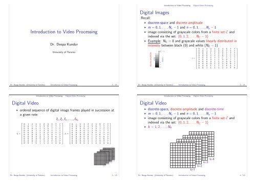
Dr. Deepa Kundur
University of Toronto
Dr. Deepa Kundur (University of Toronto) Introduction to Video Processing 1 / 23
Digital Video
Introduction to Video Processing Digital Video Processing
◮ ordered sequence of digital image frames played in succession at
a given rate:
I1, I2, I3, . . . , INF
⎡
⎢
I1 = ⎢
⎣
0 1 2 2 2 2 3 5 7 7
0 0 1 2 2 3 5 7 7 7
0 0 0 1 2 3 5 7 7 7
0 0 0 2 2 3 6 7 7 7
0 0 0 2 2 3 7 7 7 7
0 0 0 0 1 2 5 6 7 7
0 0 0 0 1 2 3 5 6 7
0 0 0 0 1 2 3 5 6 7
0 0 0 1 1 1 2 4 5 7
0 0 1 1 1 1 2 3 4 6
⎤
⎡
⎥ ⎢
⎥ ⎢
⎥ ⎢
⎥ ⎢
⎥ ⎢
⎥ ⎢
⎥ ⎢
⎥ , I2 = ⎢
⎥ ⎢
⎥ ⎢
⎥ ⎢
⎥ ⎢
⎥ ⎢
⎦ ⎣
0 1 2 2 2 2 3 5 7 7
0 0 0 2 2 3 5 7 7 7
0 0 0 0 2 3 5 7 7 7
0 0 0 0 2 3 6 7 7 7
0 0 0 0 2 3 7 7 7 7
0 0 0 0 0 1 5 6 7 7
0 0 0 0 0 1 3 5 6 7
0 0 0 0 0 1 3 5 6 7
0 0 0 0 1 1 2 4 5 7
0 0 0 0 1 1 2 3 4 6
k=1
⎤
⎥
⎦
· · ·
k=4
k=3
k=2
Dr. Deepa Kundur (University of Toronto) Introduction to Video Processing 3 / 23
Digital Images
Recall:
Introduction to Video Processing Digital Video Processing
◮ discrete-space and discrete-amplitude
◮ m = 0, 1, . . . , Nx − 1 and n = 0, 1, . . . , Ny − 1
◮ image consisting of grayscale colors from a finite set C and
indexed via the set: {0, 1, 2, . . . , NC − 1}
◮ Example: NC = 8 and grayscale values linearly distributed in
intensity between black (0) and white (NC − 1)
discrete-amplitude
color
.
.
.
2
1
0
I-value
continuous-amplitude
1.0
color
0.5
0.0
I-value
⎡
⎢
I = ⎢
⎣
0 1 2 2 2 2 3 5 7 7
0 0 1 2 2 3 5 7 7 7
0 0 0 1 2 3 5 7 7 7
0 0 0 2 2 3 6 7 7 7
0 0 0 2 2 3 7 7 7 7
0 0 0 0 1 2 5 6 7 7
0 0 0 0 1 2 3 5 6 7
0 0 0 0 1 2 3 5 6 7
0 0 0 1 1 1 2 4 5 7
0 0 1 1 1 1 2 3 4 6
Dr. Deepa Kundur (University of Toronto) Introduction to Video Processing 2 / 23
Digital Video
Introduction to Video Processing Digital Video Processing
◮ discrete-space, discrete-amplitude and discrete-time
◮ m = 0, 1, . . . , Nx − 1 and n = 0, 1, . . . , Ny − 1
◮ image consisting of grayscale colors from a finite set C and
indexed via the set: {0, 1, 2, . . . , NC − 1}
◮ k = 1, 2, . . . , NF
k=1
k=4
k=3
k=2
Dr. Deepa Kundur (University of Toronto) Introduction to Video Processing 4 / 23
⎤
⎥
⎦

Digital Video
Introduction to Video Processing Digital Video Processing
◮ basic unit of processing is called the pixel denoted by its location
in the 3-D video sequence using k, m, n.
◮ Ik(m, n) ∈ C.
◮ Note: I2(0, 2) is shown below:
(0,2)
k=1
k=4
k=3
k=2
Dr. Deepa Kundur (University of Toronto) Introduction to Video Processing 5 / 23
Spatial Correlation
Assuming real images:
Introduction to Video Processing Digital Video Processing
RI (i, j) =
I (m, n)I (m − i, n − j)
m,n
◮ “high” correlation can mean that pixels within a neighborhood
have similar colors
◮ “zero” correlation can mean that adjacent pixels are unrelated in
color
Dr. Deepa Kundur (University of Toronto) Introduction to Video Processing 7 / 23
Introduction to Video Processing Digital Video Processing
Digital Video Processing
◮ Often makes use of the correlation amongst pixels:
◮ spatially
◮ temporally
Dr. Deepa Kundur (University of Toronto) Introduction to Video Processing 6 / 23
Spatial Correlation
Introduction to Video Processing Digital Video Processing
natural image with positive
spatial correlation
random image with zero
correlation
Dr. Deepa Kundur (University of Toronto) Introduction to Video Processing 8 / 23

Spatial Correlation
Introduction to Video Processing Digital Video Processing
maximum correlation maximum correlation
Dr. Deepa Kundur (University of Toronto) Introduction to Video Processing 9 / 23
Temporal Processing
Introduction to Video Processing Digital Video Processing
h0 x + h1 x + h2 x + h3 x =
Dr. Deepa Kundur (University of Toronto) Introduction to Video Processing 11 / 23
Spatial Processing
h-1,-1x h
-1,0
x
h-1,1 x
Introduction to Video Processing Digital Video Processing
+h 0,-1x
+
+
+
h 1,-1 x
+ h 0,0 x + h1,0 x
+ h 0,1 x + h1,1 x
Dr. Deepa Kundur (University of Toronto) Introduction to Video Processing 10 / 23
Temporal Correlation
Introduction to Video Processing Digital Video Processing
maximum correlation uncorrelated
Dr. Deepa Kundur (University of Toronto) Introduction to Video Processing 12 / 23
=

Introduction to Video Processing Digital Video Processing
Types of Digital Video Processing
◮ FIR filtering
◮ denoising
◮ enhancing
◮ restoration
◮ object identification
◮ motion detection
◮ compression
◮ · · ·
Dr. Deepa Kundur (University of Toronto) Introduction to Video Processing 13 / 23
Edge Detection
Introduction to Video Processing Edge Detection
Q: Why conduct edge detection?
A: Applying edge detection
◮ identifies discontinuities or sharp boundaries within an image
which can significantly help in later interpretation of the image
◮ reduces the volume of data making subsequent processing (often
involving image analysis or computer vision) simpler
Dr. Deepa Kundur (University of Toronto) Introduction to Video Processing 15 / 23
Edge Detection
Introduction to Video Processing Edge Detection
◮ process of identifying “sharp” changes in brightness
◮ Why is this important?
◮ detects changes in properties of the world
◮ the image formation process in many applications (seismology,
photography, radar, microscopy, ultrasound, magnetic resonance
imaging, etc.) is such that changes in brightness can relate to:
◮ severe changes in depth/distance
◮ discontinuities in surface orientation
◮ changes in material properties
◮ variations in scene illumination
◮ boundaries of an object
Dr. Deepa Kundur (University of Toronto) Introduction to Video Processing 14 / 23
Introduction to Video Processing Edge Detection
Gradient-Based Edge Detection
1. Compute gradient of image to characterize color changes amongst
neighboring pixels
◮ a gradient measures the difference in values amongst adjacent
pixels
2. Compute edge strength by taking the magnitude of the gradient
◮ a gradient is more pronounced when the difference amongst
adjacent pixel values is larger
3. Threshold to identify where the edges exist
◮ a smaller/larger threshold will detect fewer/more edges
◮ this “cleans up” the image resulting in a binary result
4. Edge thinning
◮ results in edges that are only one pixel in width making
subsequent interpretation easier
Dr. Deepa Kundur (University of Toronto) Introduction to Video Processing 16 / 23

Introduction to Video Processing Edge Detection
One-Dimensional Example
EDGE
(a) (b)
(c)
THRESHOLD 1
EDGE EDGE
(d)
THRESHOLD 2
(a) Signal, (b) Signal Gradient, (c) Absolute Value of Signal Gradient with Edge
Detection using Threshold 1, (d) Absolute Value of Signal Gradient with Edge
Detection using Threshold 2.
Dr. Deepa Kundur (University of Toronto) Introduction to Video Processing 17 / 23
Sobel Edge Detection
Consider Gx(m, n):
Introduction to Video Processing Edge Detection
Gx(m, n) = Mx(m, n) ∗ Ik(m, n)
=
+1
+1
i=−1 j=−1
Mx(i, j)Ik(m − i, n − k)
= −1 · Ik(m + 1, n + 1) + 1 · Ik(m + 1, n − 1)
−2 · Ik(m, n + 1) + 2 · Ik(m, n − 1)
−1 · Ik(m − 1, n + 1) + 1 · Ik(m − 1, n − 1)
= [Ik(m + 1, n − 1) + 2Ik(m, n − 1) + Ik(m − 1, n − 1)]
− [Ik(m + 1, n + 1) + 2Ik(m, n + 1) + Ik(m − 1, n + 1)]
Dr. Deepa Kundur (University of Toronto) Introduction to Video Processing 19 / 23
Sobel Edge Detection
Introduction to Video Processing Edge Detection
◮ Assume an intensity (i.e., grayscale) image.
◮ Two gradients are computed in the horizontal and vertical directions
denoted Gx and Gy , respectively.
◮ The gradients are computed as follows:
Gx(m, n) = Mx(m, n)∗Ik(m, n)
Gy (m, n) = My (m, n)∗Ik(m, n)
where ∗ represents 2-D convolution of the image Ik with the masks:
⎡
−1
Mx = ⎣ −2
0
0
⎤ ⎡
+1
+1
+2 ⎦My = ⎣ 0
+2
0
⎤
+1
0 ⎦
−1 0 +1
−1 −2 −1
◮ Mx and My represent 2-D FIR filters.
Dr. Deepa Kundur (University of Toronto) Introduction to Video Processing 18 / 23
Computation of Gx
(m,n)
(horiz,vert)
Introduction to Video Processing Edge Detection
+1 +2 +1
-1 -2 -1
+1 +2 +1
-1 -2 -1
+1 +2 +1
-1 -2 -1
+1 +2 +1
-1 -2 -1
|Gx(m, n)| is large if (m, n) lies on the boundary of a horizontal edge.
Dr. Deepa Kundur (University of Toronto) Introduction to Video Processing 20 / 23

Computation of Gy
(m,n)
(horiz,vert)
Introduction to Video Processing Edge Detection
-1
-2
-1
+1
+2
+1
-1
-2
-1
+1
+2
+1
-1
-2
-1
+1
+2
+1
Similarly |Gy(m, n)| is large if (m, n) lies on the boundary of a
vertical edge.
Dr. Deepa Kundur (University of Toronto) Introduction to Video Processing 21 / 23
Introduction to Video Processing Edge Detection
Magnitude and Thresholding
Dr. Deepa Kundur (University of Toronto) Introduction to Video Processing 23 / 23
-1
-2
-1
+1
+2
+1
Introduction to Video Processing Edge Detection
Magnitude and Thresholding
Compute |G(m, n)| = Gx 2 (m, n) + Gy 2 (m, n)
◮ If |G(m, n)| > T then (m, n) lies at an edge boundary.
◮ Otherwise, (m, n) is not at a boundary.
Dr. Deepa Kundur (University of Toronto) Introduction to Video Processing 22 / 23