Using SPSS Statistics Syntax - University of Massachusetts Amherst
Using SPSS Statistics Syntax - University of Massachusetts Amherst
Using SPSS Statistics Syntax - University of Massachusetts Amherst
You also want an ePaper? Increase the reach of your titles
YUMPU automatically turns print PDFs into web optimized ePapers that Google loves.
https://udrive.oit.umass.edu/statdata/spss.zip<br />
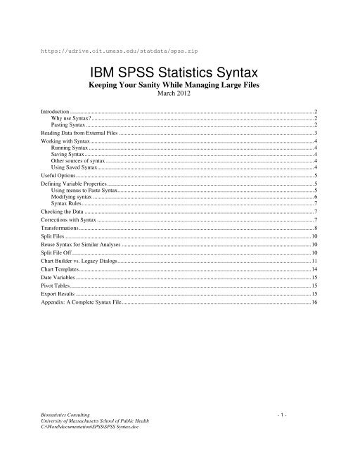
IBM <strong>SPSS</strong> <strong>Statistics</strong> <strong>Syntax</strong><br />
Keeping Your Sanity While Managing Large Files<br />
March 2012<br />
Introduction .......................................................................................................................................................................... 2<br />
Why use <strong>Syntax</strong>? ........................................................................................................................................................... 2<br />
Pasting <strong>Syntax</strong> ............................................................................................................................................................... 2<br />
Reading Data from External Files ........................................................................................................................................ 3<br />
Working with <strong>Syntax</strong> ............................................................................................................................................................ 4<br />
Running <strong>Syntax</strong> ............................................................................................................................................................. 4<br />
Saving <strong>Syntax</strong> ................................................................................................................................................................ 4<br />
Other sources <strong>of</strong> syntax ................................................................................................................................................. 4<br />
<strong>Using</strong> Saved <strong>Syntax</strong> ....................................................................................................................................................... 4<br />
Useful Options ...................................................................................................................................................................... 5<br />
Defining Variable Properties ................................................................................................................................................ 5<br />
<strong>Using</strong> menus to Paste <strong>Syntax</strong>......................................................................................................................................... 5<br />
Modifying syntax .......................................................................................................................................................... 6<br />
<strong>Syntax</strong> Rules .................................................................................................................................................................. 7<br />
Checking the Data ................................................................................................................................................................ 7<br />
Corrections with <strong>Syntax</strong> ....................................................................................................................................................... 7<br />
Transformations .................................................................................................................................................................... 8<br />
Split Files ............................................................................................................................................................................ 10<br />
Reuse <strong>Syntax</strong> for Similar Analyses .................................................................................................................................... 10<br />
Split File Off ....................................................................................................................................................................... 10<br />
Chart Builder vs. Legacy Dialogs ....................................................................................................................................... 11<br />
Chart Templates .................................................................................................................................................................. 14<br />
Date Variables .................................................................................................................................................................... 15<br />
Pivot Tables ........................................................................................................................................................................ 15<br />
Export Results .................................................................................................................................................................... 15<br />
Appendix: A Complete <strong>Syntax</strong> File .................................................................................................................................... 16<br />
Biostatistics Consulting - 1 -<br />
<strong>University</strong> <strong>of</strong> <strong>Massachusetts</strong> School <strong>of</strong> Public Health<br />
C:\Word\documentation\<strong>SPSS</strong>\<strong>SPSS</strong> <strong>Syntax</strong>.doc
Introduction<br />
Information presented here is intended for <strong>SPSS</strong> <strong>Statistics</strong> version 17 or higher. The <strong>Syntax</strong> and principles<br />
apply to earlier <strong>SPSS</strong> versions as well, but the Graphical User Interface items have changed significantly<br />
over releases, so these cannot necessarily be used in earlier versions.<br />
Most things you do in <strong>SPSS</strong> <strong>Statistics</strong> have an associated set <strong>of</strong> commands (syntax). You can begin<br />
learning syntax by looking at the syntax generated by your menu choices. The generated syntax is visible in<br />
your output window:<br />
Why use <strong>Syntax</strong>?<br />
<strong>Syntax</strong> provides a valuable record <strong>of</strong> what you did. In particular, if you use data transformations such as<br />
Compute or Recode from the menu system, it is difficult to trace how new variables are defined or how<br />
existing variables are changed. Saving the syntax for such data transformations provides the necessary<br />
documentation <strong>of</strong> how new variables were defined. It also enables you to check whether you did<br />
everything you intended to, make corrections easily, and insures that you will be able to duplicate the<br />
computations, should that be necessary.<br />
If you need to do the same (or very similar) analysis many times, you can do it more quickly and with<br />
fewer opportunities for errors by using syntax. Once you have written and checked that the syntax is doing<br />
what you want, you can run it repeatedly, in this or future <strong>SPSS</strong> <strong>Statistics</strong> sessions, without having to make<br />
any menu choices. You can make minor modifications without having to go through the menus again. The<br />
syntax can include a whole series <strong>of</strong> procedures.<br />
<strong>Syntax</strong> is not dependent on your operating system; thus, analyses started on one machine can easily be recreated<br />
and continued on another machine by transferring the syntax and data files.<br />
Finally, some advanced features are not available from the menus. For example, General Linear Models<br />
can do factorial and repeated measures models from the menus. For nested models, you must use syntax.<br />
Pasting <strong>Syntax</strong><br />
The easiest way to begin using syntax is to complete all your choices and options from the menus, and click<br />
Paste. A <strong>Syntax</strong> window will be opened, showing the syntax generated by the choices you made.<br />
Most <strong>SPSS</strong> <strong>Statistics</strong> dialog boxes have a Paste button. <strong>Using</strong> Paste, you can create a syntax file for your<br />
entire analysis.<br />
The Define Variable Properties dialog can be used to Paste <strong>Syntax</strong> for defining missing values, variable<br />
labels, value labels, formats, and other variable attributes. Changes made directly in the Variable View<br />
window do not generate syntax, so should be avoided if you are trying to collect syntax.<br />
Biostatistics Consulting - 2 -<br />
<strong>University</strong> <strong>of</strong> <strong>Massachusetts</strong> School <strong>of</strong> Public Health<br />
C:\Word\documentation\<strong>SPSS</strong>\<strong>SPSS</strong> <strong>Syntax</strong>.doc
Reading Data from External Files<br />
The gss93.dat data is a small subset <strong>of</strong> a large social/demographic survey. You can get information about<br />
it, and download the data file from http://www.umass.edu/statdata/statdata/data. Use the following variable<br />
names and locations to read the data:<br />
ID - integer in columns 1-4<br />
MARSTAT - Marital Status - columns 5<br />
AGE - columns 6-7<br />
DEGREE. - columns 8-9<br />
SEX - column 10<br />
ETHNIC - column 11<br />
RELIG - column 12<br />
CAPPUN - column 13<br />
GUNLAW - column 14<br />
SEXEDUC - column 15<br />
LETDIE - column 16<br />
READNEWS - column 17<br />
TVNEWS - column 18<br />
TVPBS - column 19<br />
BIGBAND - column 20<br />
BLUEGRAS - column 21<br />
CW - column 22<br />
BLUES - column 23<br />
MUSICAL - column 24<br />
FOLK - column 25<br />
JAZZ - column 26<br />
Observe that the variables are not delimited by blanks (or anything else). Also, some missing information<br />
has been left blank. Therefore, the data cannot be read as freefield. However, since the variables are<br />
aligned in columns, we can use Fixed Format to read this data.<br />
Choose File/Read Text Data. Go through the Import data wizard dialogs, filling them in as follows:<br />
Look In: Folder where you saved the file. For the workshop, select Desktop →<strong>SPSS</strong>work<br />
Filename: gss93.dat<br />
Files <strong>of</strong> type: Text (*.txt, *.dat)<br />
Click Open<br />
Does your text file match a predefined format? No. Click Next<br />
How are your variables arranged? Fixed width<br />
Are variable names included at top <strong>of</strong> your file? No. Click Next<br />
First case <strong>of</strong> data begins on which line? 1<br />
How many lines represent a case? 1<br />
How many cases do you want to import? All the cases. Click Next<br />
The vertical lines in data represent breakpoints between variables? Click between the<br />
numbers to separate variables, using the variable location information above. Click Next<br />
Specification for variable selected in data preview? Click a column heading in the data preview<br />
to select it, type the variable name for it in the Variable Name box, using the names listed above.<br />
Repeat for each columns. Click Next<br />
Would you like to save the file format? No<br />
Would you like to paste the syntax? Yes. Click Finish<br />
A <strong>Syntax</strong> window opens, with the <strong>SPSS</strong> <strong>Statistics</strong> command equivalent <strong>of</strong> the menu choices you made.<br />
Biostatistics Consulting - 3 -<br />
<strong>University</strong> <strong>of</strong> <strong>Massachusetts</strong> School <strong>of</strong> Public Health<br />
C:\Word\documentation\<strong>SPSS</strong>\<strong>SPSS</strong> <strong>Syntax</strong>.doc
Working with <strong>Syntax</strong><br />
Running <strong>Syntax</strong><br />
To run all or part <strong>of</strong> the commands in the <strong>Syntax</strong> window:<br />
From the <strong>SPSS</strong> <strong>Statistics</strong> <strong>Syntax</strong> editor menu → Run<br />
Choose:<br />
All (to run everything in the syntax window)<br />
Selection (runs only highlighted syntax)<br />
To end (runs syntax from cursor position to end)<br />
Saving <strong>Syntax</strong><br />
In order to use the same syntax in a future <strong>SPSS</strong> <strong>Statistics</strong> session, you need to save it.<br />
From the <strong>SPSS</strong> <strong>Statistics</strong> <strong>Syntax</strong> editor window → File → Save As<br />
Save in: choose a drive or directory<br />
<strong>SPSS</strong>work)<br />
(for the workshop, use Desktop →<br />
Filename: gss93<br />
Save as type:<strong>SPSS</strong> <strong>Statistics</strong>(*.sps)<br />
Other sources <strong>of</strong> syntax<br />
You can copy syntax from the log output in the viewer and paste it into a syntax window.<br />
Finally, if all else fails, all <strong>of</strong> the syntax from each <strong>SPSS</strong> <strong>Statistics</strong> session is saved in the <strong>SPSS</strong> journal file,<br />
statistics.jnl. The name and default location <strong>of</strong> this file varies depending on your version <strong>of</strong><br />
Windows, and your version <strong>of</strong> <strong>SPSS</strong> <strong>Statistics</strong>. Look in Edit Options File Locations (or General)<br />
to see where it is on your system. → →<br />
If you want to extract syntax for a session from the journal, you must do this promptly, as it will become<br />
increasingly difficult to identify as syntax from later sessions is appended. Alternatively, if you have set<br />
your journal option to overwrite, the syntax from a session is destroyed as soon as you re-open <strong>SPSS</strong><br />
<strong>Statistics</strong>. Open the journal file with any text editor (e.g.Wordpad, Notepad, etc), and copy the syntax you<br />
want. Save the extracted syntax to your personal directory (folder), and add some comments so you can<br />
associate the commands with the corresponding output file. In line with <strong>SPSS</strong> <strong>Statistics</strong> conventions, the<br />
syntax file should have the .sps extensions. To add comments without disturbing the syntax, write the<br />
word Comment at the left margin. Then type any text you want. You can continue on as many lines as you<br />
need. The comment should not have any internal periods, but must end with a period.<br />
<strong>Using</strong> the journal is a last-ditch solution, as you will likely need to be very selective in what you take from<br />
it, and may need to do considerable editing.<br />
<strong>Using</strong> Saved <strong>Syntax</strong><br />
You can reuse syntax saved to a file in a new <strong>SPSS</strong> <strong>Statistics</strong> session.<br />
From the Menu → File → Open → <strong>Syntax</strong><br />
From the Open file dialog box:<br />
Look in: drive or directory where syntax was saved<br />
(for the workshop, use Desktop → <strong>SPSS</strong>work)<br />
Filename: gss93<br />
File <strong>of</strong> type: <strong>SPSS</strong> <strong>Statistics</strong> (*.sps)<br />
You can now run it to repeat your previous analysis or edit it if you need to make some changes.<br />
Biostatistics Consulting - 4 -<br />
<strong>University</strong> <strong>of</strong> <strong>Massachusetts</strong> School <strong>of</strong> Public Health<br />
C:\Word\documentation\<strong>SPSS</strong>\<strong>SPSS</strong> <strong>Syntax</strong>.doc
Useful Options<br />
Under Edit - Options you can choose whether dialog boxes will present variable lists using variable<br />
names or variable labels, and whether the variables in the dialog boxes will be in the file order or in<br />
alphabetic order. For large files in which the variables have been arranged in some logical order, file<br />
order is generally more useful.<br />
Under Data, you can set the 100-year interval <strong>SPSS</strong> <strong>Statistics</strong> will assume if you enter a date using only<br />
two digits for the year.<br />
You can also choose from a variety <strong>of</strong> standard table and chart formats, what is displayed or hidden in the<br />
Output, and many other features. When you make changes to Options, your latest choices are saved, and<br />
will remain in effect for future sessions.<br />
Defining Variable Properties<br />
<strong>Using</strong> menus to Paste <strong>Syntax</strong><br />
The gss93 data has several groups <strong>of</strong> variables that are coded the same way:<br />
CAPPUN, GUNLAW, SEXEDUC, LETDIE<br />
0,8,9 represent different kinds <strong>of</strong> missing values<br />
1 - Favor<br />
2 - Oppose.<br />
READNEWS, TVNEWS, TVPBS<br />
0,8,9, are missing<br />
1 - every day<br />
2 - a few times per week<br />
3 - once a week<br />
4 - rarely<br />
5 - never<br />
BIGBAND to JAZZ ( 8 variables)<br />
0,8,9 are missing<br />
1 - like very much<br />
2 - like<br />
3 - mixed feelings<br />
4 - dislike<br />
5 - dislike a lot<br />
We can make the job <strong>of</strong> defining missing values and value labels much easier by setting up a the correct<br />
values for one variable in each group, then copying it to the remaining variables.<br />
In the Define Variable Properties dialog, select MARSTAT, DEGREE to JAZZ to Scan. (Shift-Click or<br />
Control-Click are easy ways to select many variables in a dialog.) Click Continue. Define the Missing<br />
Values, Value Labels, Type, Measurement Level, Width and Decimals for each <strong>of</strong> MARSTAT to<br />
RELIG. Do NOT press OK after each variable definition. Simply click another variable and proceed with<br />
its definition. When you get to CAPPUN, after defining its properties, under Copy Properties, click To<br />
Other Variables. Select GUNLAW, SEXEDUC, LETDIE, and click Copy. Similarly, define the variable<br />
properties for the first variable from each <strong>of</strong> the other groups, and copy it to all the other variables in the<br />
group. When ALL variables properties are defined, click Paste.<br />
Biostatistics Consulting - 5 -<br />
<strong>University</strong> <strong>of</strong> <strong>Massachusetts</strong> School <strong>of</strong> Public Health<br />
C:\Word\documentation\<strong>SPSS</strong>\<strong>SPSS</strong> <strong>Syntax</strong>.doc
Here is the first the set <strong>of</strong> commands generated for the CAPPUN to LETDIE group:<br />
*cappun.<br />
VARIABLE LABELS cappun 'Capital Punishment'.<br />
MISSING VALUES cappun ( 0, 8, 9 ).<br />
VALUE LABELS cappun<br />
1 'Favor'<br />
2 'Oppose' .<br />
A similar MISSING VALUES and VALUE LABELS command is generated for each variable in the<br />
group. The VARIABLE LABELS is not copied to the other variables, but we can use the above as a model<br />
for adding VARIABLE LABELS to any additional variables that need them.<br />
Modifying syntax<br />
The generated syntax contains an identical set <strong>of</strong> MISSING VALUES and VALUE LABELS for each<br />
variable in each group, which makes it rather lengthy. You can <strong>of</strong>ten write much more compact code by<br />
generating the definition for the first variable in each group, and modifying the code to include other<br />
variables. For example the code for CAPPUN to LETDIE could be shortened to:<br />
MISSING VALUES CAPPUN TO LETDIE(0,8,9).<br />
VAR LABELS CAPPUN 'Capital Punishment'/ GUNLAW 'Gun Control'/<br />
SEXEDUC 'Sex Education'/ LETDIE 'Let Terminal Patients Die'.<br />
VALUE LABELS CAPPUN TO LETDIE 1 'FAVOR' 2 'OPPOSE'.<br />
Notice that the MISSING VALUES and VALUE LABELS commands both accept lists <strong>of</strong> variables.<br />
Groups <strong>of</strong> contiguous variables can be specified using the keyword TO; non-contiguous variables can be<br />
listed separated by blanks or commas. You can even specify variables with different definitions on a<br />
single MISSING VALUES or VALUE LABELS command, by separating them with a slash. The complete<br />
set <strong>of</strong> MISSING VALUES and VALUE LABELS might look like this:<br />
MISSING VALUES MARSTAT(9)/AGE (0,98,99)/ DEGREE (7,8,9)/<br />
RELIG(8,9)/CAPPUN TO JAZZ(0,8,9).<br />
VALUE LABELS MARSTAT 1 "Married" 2 "Widowed" 3 "Divorced"<br />
4 "Separated" 5 "Never Married" /<br />
DEGREE 0 'Less than High School' 1 'High School'<br />
2 'Junior College' 3 'Bachelor' 4 'Graduate' /<br />
SEX 1 'Male' 2 'Female' / ETHNIC 1 'White' 2 "Black" 3 'Other'/<br />
RELIG 1 'Protestant' 2 'Catholic' 3 'Jewish' 4 'None' 5 'Other'/<br />
CAPPUN TO LETDIE 1 "favor" 2 "oppose"/<br />
READNEWS TO TVPBS 1 "every day" 2 "few times per week"<br />
3 "once a week" 4 "rarely" 5 "never"/<br />
BIGBAND TO JAZZ 1 "like a lot" 2 "like" 3 "mixed"<br />
4 "dislike" 5 "dislike a lot".<br />
Upper/lower case is strictly cosmetic. You can use either apostrophes (') or quotes (") in label definitions,<br />
provided the label does not itself contain these characters – for example the label "don't know" requires<br />
quotes. Indentation is used to make code easier to read – it is not required.<br />
Select the MISSING VALUES, VAR LABELS, VALUE LABELS and FORMAT commands and Run<br />
them. Check your Output window for any error messages, and look in the Variable View window to<br />
confirm that all variables have the correct properties. When you are done, your syntax file should contain<br />
everything you need to read the gss93 text file and define all essential variable properties – GET DATA,<br />
MISSING VALUES, VAR LABELS, and VALUE LABELS commands.<br />
Biostatistics Consulting - 6 -<br />
<strong>University</strong> <strong>of</strong> <strong>Massachusetts</strong> School <strong>of</strong> Public Health<br />
C:\Word\documentation\<strong>SPSS</strong>\<strong>SPSS</strong> <strong>Syntax</strong>.doc
<strong>Syntax</strong> Rules<br />
The contents <strong>of</strong> the syntax window can be edited as with any text editor. You can add or change options to<br />
suit your needs. Use the <strong>Syntax</strong> Reference Manual to look up details <strong>of</strong> command options.<br />
The general rules are:<br />
• commands begin at the left margin<br />
• continuation lines are indented at least one space<br />
• text must not be longer than 80 characters on any line.<br />
• each command must end with a period.<br />
• options or different parts <strong>of</strong> a command are usually separated by a slash (/)<br />
• Variable lists <strong>of</strong> the form VAR1 TO VARn imply that the command applies to all the variables in<br />
the data file between VAR1 and VARn (inclusive). The order implied is data file order, not<br />
alphabetic order, regardless <strong>of</strong> the Display Order setting in Edit/Options.<br />
• You can use variable lists <strong>of</strong> the form VARa TO VARk, VARm, VARp TO VARs to make lists<br />
that combine groups <strong>of</strong> contiguous and non-contiguous variables.<br />
If you Copy and Paste a command, be sure to start the selection at the beginning <strong>of</strong> the command (where it<br />
is at the left margin), and go to the period at the end. (Pasted syntax usually has the period on a line by<br />
itself.) Then you can make modifications between these two points, keeping all intermediate lines indented,<br />
and leaving any slashes where they are. Use the dialogs to generate the <strong>Syntax</strong> as much as possible, so you<br />
can use it as a model. If in doubt, you can check the precise syntax <strong>of</strong> any command in Online Help.<br />
Checking the Data<br />
Having created a new <strong>SPSS</strong> <strong>Statistics</strong> file, we should do some simple descriptive statistics to make sure that<br />
the data has been read correctly. All the variables other than age are categorical, so we will begin with<br />
Frequencies on these variables.<br />
Run Frequencies on all the variables except ID and Age. When you’ve filled out the dialog, click Paste.<br />
Observe that the Frequencies command is added to your <strong>Syntax</strong> window, but the command is not run. As<br />
before, pasted syntax is considerably more verbose than necessary. It particular, each selected variable is<br />
named. If we were to write our own FREQUENCIES command we would use the TO convention to select<br />
contiguous variables:<br />
FREQUENCIES VARIABLES=MARSTAT, DEGREE TO JAZZ.<br />
To run the Frequencies from the <strong>Syntax</strong> window, place the cursor anywhere within the Frequencies<br />
command. Notice the blue triangle marking the line with the cursor. If the command takes more than one<br />
line, an indicator shows the beginning and end <strong>of</strong> the command. Choose Run/Selection (or click the right<br />
facing triangle on the toolbar).<br />
Save the syntax file as gss93.sps, and the data file as gss93.sav.<br />
Corrections with <strong>Syntax</strong><br />
Looking over the Frequencies output, and comparing it to the data dictionary, we realize that something is<br />
seriously wrong! Variables DEGREE, SEX, ETHNIC, and LETDIE have many cases with values that are<br />
not in the codebook. Checking the codebook we realize that DEGREE should have been read from column<br />
8 only, not columns 8-9. As a result <strong>of</strong> this error, all the subsequent variables were read from the wrong<br />
location. In addition, we left out one variable, CLASSICL, which should be between MUSICAL and<br />
FOLK. We will need to re-read the data file using the correct locations for the variables.<br />
Biostatistics Consulting - 7 -<br />
<strong>University</strong> <strong>of</strong> <strong>Massachusetts</strong> School <strong>of</strong> Public Health<br />
C:\Word\documentation\<strong>SPSS</strong>\<strong>SPSS</strong> <strong>Syntax</strong>.doc
We have already spent considerable time naming the variables, defining missing values, value labels, etc.<br />
<strong>Using</strong> the dialogs alone, we would have to start all over! In addition to the burden <strong>of</strong> going through all the<br />
work again, we risk making other mistakes. <strong>Using</strong> the saved syntax it is easy to make the necessary<br />
correction, while preserving the parts we got right.<br />
In the gss93.sps syntax window, go to the GET DATA command, and change the column locations <strong>of</strong> all<br />
the variables, starting with DEGREE 7-7. Note that <strong>SPSS</strong> <strong>Statistics</strong> starts numbering positions at 0, rather<br />
than 1. As a result, all variable locations are one less than on the codebook. Insert CLASSICL 23-23<br />
between MUSICAL and FOLK.<br />
Look through the remaining commands to see whether these corrections have further ramifications. Note<br />
that the MISSING VALUES, VAR LABELS, and VALUE LABELS are correct for all previously defined<br />
variables. Add a VAR LABEL for CLASSICL. If you defined MISSING VALUES and VALUE<br />
LABELS using the list BIGBAND TO JAZZ, the newly defined variable CLASSICL is included in those<br />
commands; otherwise you'll need to add MISSING VALUES and VALUE LABELS for the new variable.<br />
The Frequencies command generated by Paste lists variables individually. You need to add CLASSICL to<br />
that list in the desired location, or change the list to the more compact version DEGREE TO JAZZ. When<br />
you are finished, save the revised syntax file, and choose Run/All. If the Frequencies output now shows<br />
that the data is correct, Save the datafile, gss93.sav, and the modified syntax file, gss93.sps.<br />
Transformations<br />
Even if you don't need to use syntax for most purposes, if you create or recode variables or do any<br />
substantive data transformations, you should save the syntax. Without it you will have a data file with a<br />
bunch <strong>of</strong> variables without a record <strong>of</strong> how they were created, nor any evidence that they are what they<br />
were intended to be. It will be impossible to do any troubleshooting, should the need arise. Furthermore, if<br />
for any reason you need to start again, the saved syntax can save you much time and grief.<br />
The gss93 survey contains four variables that ask the respondents' view on some social issues. A response<br />
<strong>of</strong> "Favor" to three <strong>of</strong> the questions, GUNLAW, SEXEDUC, LETDIE, and a response <strong>of</strong> "Oppose" to<br />
CAPPUN is considered to be at the "socially liberal" end <strong>of</strong> the spectrum. The opposite set <strong>of</strong> responses<br />
will be considered "socially conservative". Our task it to create an "index" variable that will score each<br />
respondent on a social outlook scale.<br />
We need to first make sure the four social issue questions are coded in the same "direction"; three <strong>of</strong> the<br />
four have codes that can be interpreted as 1 for "liberal" and 2 for "conservative". The codes for CAPPUN<br />
need to be reversed. When the four questions are coded in the same direction, counting the number <strong>of</strong> 1's<br />
for each respondent will give a 0-4 score, with 0 being most "conservative", and 4 most "liberal".<br />
Biostatistics Consulting - 8 -<br />
<strong>University</strong> <strong>of</strong> <strong>Massachusetts</strong> School <strong>of</strong> Public Health<br />
C:\Word\documentation\<strong>SPSS</strong>\<strong>SPSS</strong> <strong>Syntax</strong>.doc
To reverse the coding for CAPPUN, on the Data View screen:<br />
From the Transform menu, Select:<br />
Recode→Into Different Variables<br />
Select CAPPUN and move it to Input Variable->Output Variable box.<br />
Type a new name, say CAPPUNR, in the Output Variable name box.<br />
Optionally, type a Label for the new variable.<br />
Click Change.<br />
Click Old and New Values.<br />
Old Value 1; New Value 2; Click Add.<br />
Old Value 2; New Value 1; Click Add.<br />
Click System or User-Missing on the left side,<br />
Copy Old Values on the right side; Click Add.<br />
Click Continue.<br />
Click Paste.<br />
You should get the following syntax:<br />
RECODE cappun (1=2) (2=1) (MISSING=Copy) INTO cappunr .<br />
VARIABLE LABELS cappunr 'Capital Punishment Reversed'.<br />
EXECUTE .<br />
Add a Value Labels command for the new variable CAPPUNR to the syntax file.<br />
Select and Run the syntax segment that creates the new variable CAPPUNR. Run Frequencies on both<br />
CAPPUN and CAPPUNR to check that the coding has been reversed as intended and all missing values<br />
and labels are correct.<br />
When CAPPUNR has been correctly defined you are ready to create the "index" that counts the number <strong>of</strong><br />
"liberal" responses to the four questions. On the Data View screen menu:<br />
Select Transform→Count Values within Cases<br />
Type a name for the new variable in Target Variable: LIBSCORE<br />
Type a label in the Target Label box: Liberal Social View Score<br />
Select the four variables: GUNLAW, SEXEDUC, LETDIE, CAPPUNR. Do NOT<br />
select CAPPUN!<br />
Click the arrow to move the selected variables into the Numeric Variables box.<br />
Click Define Values.<br />
On the left side, select Value and type 1 into the Value box.<br />
Click Add to move it to the Values to Count box.<br />
Click Continue.<br />
Click Paste.<br />
Here is the pasted syntax:<br />
COUNT libscore = cappunr gunlaw sexeduc letdie (1) .<br />
VARIABLE LABELS libscore 'Liberal Views Score' .<br />
EXECUTE .<br />
Add VALUE LABELS for the new variable, LIBSCORE, to define 0 as "Most Conservative" and 4 as<br />
"Most Liberal". Select and run the newly added syntax.<br />
You now have a complete syntax file for reading the gss93.dat data file, defining new variables, and setting<br />
up missing values and labels for all variables. You can do a bit <strong>of</strong> clean-up to remove extraneous<br />
commands (if you pasted some things you didn't intend) put things in sensible order and add some<br />
comments. You can safely remove all but the last EXECUTE. Save the final syntax file, gss93.sps.<br />
Biostatistics Consulting - 9 -<br />
<strong>University</strong> <strong>of</strong> <strong>Massachusetts</strong> School <strong>of</strong> Public Health<br />
C:\Word\documentation\<strong>SPSS</strong>\<strong>SPSS</strong> <strong>Syntax</strong>.doc
Split Files<br />
Split File is very useful when you want to repeat a series <strong>of</strong> analyses for several subgroups. For example,<br />
suppose you want to test whether the average age <strong>of</strong> males differs according to their "liberal" score. You<br />
will then want to do the same for the females. You also want to display the comparisons with bar graphs.<br />
You could accomplish this by using Data→Select Cases to select the males and run the analysis, then<br />
select the females and re-run the same analyses. But it would be quicker and simpler to use Split Files. On<br />
the Data Editor menu:<br />
Data→Split File.<br />
Click Compare Groups or Organize Output by Groups<br />
From the list <strong>of</strong> variables, Select SEX<br />
Click the arrow to move SEX into the Groups Based on Box.<br />
(Notice that on the bottom <strong>of</strong> the dialog, the Sort the File button is on. In order to use Split Files,<br />
the data file must be sorted on the grouping variable. )<br />
Click Paste.<br />
To test for differences in age among the 5 values <strong>of</strong> the liberal beliefs score, select<br />
Analyze→Compare Means→Oneway ANOVA.<br />
Select AGE; Click the arrow to move it to Dependent List<br />
Select LIBSCORE; Click the arrow to move it to Factor.<br />
Click Options.<br />
Check Descriptives.<br />
Click Continue.<br />
Click Paste.<br />
To make the bar graphs, select<br />
Graphs→Chart Builder (do we need to define variables??) →Bar.<br />
Drag Bar Chart from the Gallery to the Chart Preview area<br />
Drag AGE to the y-axis.<br />
** Right_Click LIBSCORE; Select Ordinal.<br />
Drag LIBSCORE to the x-axis.<br />
Optionally, under the Title tab, add a title.<br />
Click Paste.<br />
Now Select and Run these commands, beginning with Split File. Note that the two graphs have different<br />
scales, and are underneath each other so they are not easily compared visually. You can get better visual<br />
comparisons by turning Split Files Off and using Column Panels or Clustering.<br />
Reuse <strong>Syntax</strong> for Similar Analyses<br />
If you want to repeat the above tests and charts for the individual opinion questions (GUNLAW,<br />
SEXEDUC, LETDIE), you can modify the syntax generated above. Copy the ONEWAY, GPL and<br />
GGRAPH syntax and Paste it below the original. Change LIBSCORE to GUNLAW in each procedure<br />
(there is one reference in Oneway, one in GGRAPH, three in GPL (2 in DATA, 1 in ELEMENT)). If you<br />
used a TITLE, you'll need to change that also. Now you can run the identical analysis for this variable.<br />
Split File Off<br />
Split File stays in effect until you turn it <strong>of</strong>f. To turn Split File <strong>of</strong>f, on the Data sheet menu select:<br />
Data→Split File<br />
Click Analyze All Cases.<br />
Click Paste<br />
Run the SPLIT FILE OFF command from the <strong>Syntax</strong> window.<br />
Biostatistics Consulting - 10 -<br />
<strong>University</strong> <strong>of</strong> <strong>Massachusetts</strong> School <strong>of</strong> Public Health<br />
C:\Word\documentation\<strong>SPSS</strong>\<strong>SPSS</strong> <strong>Syntax</strong>.doc
Chart Builder vs. Legacy Dialogs<br />
<strong>SPSS</strong> <strong>Statistics</strong> has two distinct set <strong>of</strong> graphing routines, Chart Builder and Legacy Dialogs. Although<br />
there is some overlap between their functionality, each <strong>of</strong>fers some choices not available in the other.<br />
Where they overlap there is no general rule for which procedure to use. A few observations:<br />
• To get side-by-side graphs for visual comparison, use<br />
o Chart Builder with a Columns Panel variable<br />
o Legacy Dialog with a COLUMN variable<br />
• To get line charts with proportional axis for scale variables with unequal spacing, use Chart<br />
Builder. See example 1.<br />
• Legacy Dialogs can create multiple-variable clustered bar charts. Chart Builder does not have this<br />
feature. See Example 2.<br />
• Chart Builder lets you choose the base for computing percentages. Legacy Dialogs does not. See<br />
Example 3.<br />
You may have to experiment with both procedures to see which is better for any given situation.<br />
Example 1: Proportional axis scale.<br />
In order to illustrate what happens with unequally spaced scale variables, we need to create such a variable.<br />
We will do this by computing the square <strong>of</strong> LIBSCORE. We will call the new variable LIBSCOR2. It will<br />
have codes 0,1,4,9, and 16. The syntax is:<br />
COMPUTE LIBSCOR2=LIBSCORE**2.<br />
Notice that LIBSCOR2 is a scale variable. Now let's make a line graph <strong>of</strong> average AGE against<br />
LIBSCOR2, comparing Legacy Dialog and Chart Builder results. (The same is true for Bar graphs, but<br />
there is less <strong>of</strong> an expectation for bar spacing to reflect a scale.) From the Graph menu:<br />
Legacy Dialogs →Line<br />
Select Simple<br />
Select Summaries for Groups <strong>of</strong> Cases<br />
Click Define<br />
Select Other Summary Function<br />
Select Age<br />
Click the arrow to put Mean(Age) into the Variable box<br />
Select Libscor2<br />
Click the arrow to move it to the Category Axis box<br />
Click Paste<br />
Run the generated GRAPH command. Observe that the values <strong>of</strong> 0,1,4,9, and 16 are equally spaced on the<br />
x-axis, even though the measurement level <strong>of</strong> LIBSCOR2 is Scale. If the values <strong>of</strong> the x-variable have any<br />
quantitative meaning you would likely want the x-scale to reflect the magnitude <strong>of</strong> the x-variable.<br />
Compare the results to Chart Builder:<br />
Graphs Chart Builder Line<br />
Drag Simple Line to the Preview area<br />
Drag Age to the y-axis.<br />
Drag Libscor2 to x-axis. (If it does not have the ruler icon, right-click and select<br />
Scale.)<br />
Click Paste<br />
→ →<br />
Run the generated commands. The x-axis is now proportional to the values <strong>of</strong> LIBSCOR2.<br />
Re-do the graph, but this time right-click Libscor2 and select Ordinal, rather than Scale. Compare the<br />
resulting graphs for the two commands.<br />
Biostatistics Consulting - 11 -<br />
<strong>University</strong> <strong>of</strong> <strong>Massachusetts</strong> School <strong>of</strong> Public Health<br />
C:\Word\documentation\<strong>SPSS</strong>\<strong>SPSS</strong> <strong>Syntax</strong>.doc
Example 2: Multi-variable clustered bars.<br />
We would like to make a graph comparing the percent in favor <strong>of</strong> the 4 social issue questions among males<br />
to the percent in favor among females. <strong>Using</strong> Legacy Dialogs,<br />
Legacy Dialogs Bar<br />
Click Clustered<br />
Click Summaries <strong>of</strong> Separate Variables<br />
Click Define<br />
Select CAPPUN, GUNLAW, SEXEDUC, LETDIE<br />
Click the arrow to move them to the Bars Represent box<br />
Click Change Summary<br />
Select Percentage Inside<br />
Enter 1 in both the Low and High boxes<br />
Click Continue<br />
Select SEX<br />
Click the arrow to move it to the Category Axis box<br />
Click Titles<br />
Line 1: Percent in Favor<br />
Line 2: By Gender<br />
Click Continue<br />
→<br />
Click Paste<br />
Run the Graph syntax.<br />
Chart Builder does not have a feature for displaying several variables on one chart.<br />
Example 3: Choosing the base for percents<br />
Let's take another look at percent in favor <strong>of</strong> gun control laws, comparing the two genders' opinions.<br />
Legacy Dialogs Bar<br />
Click Clustered<br />
Click Summaries <strong>of</strong> Groups <strong>of</strong> Cases<br />
Click Define<br />
Under "Bars Represent", select % <strong>of</strong> Cases<br />
Select GUNLAW<br />
Click the arrow to move it to the Category Axis box<br />
Select SEX<br />
Click the arrow to move it to the Define Clusters By box<br />
Click Titles<br />
Line 1: Opinion on Gun Control Law<br />
Line 2: By Gender<br />
Click Continue<br />
Click Paste<br />
→<br />
Observe that when we choose "% <strong>of</strong> Cases" we get no information on (or control over) what the base for<br />
the percents is. In fact, what we get is percent in favor or opposed to gun control laws, within gender.<br />
Suppose we want to look at "what percent <strong>of</strong> those in favor or opposed are male/female"? <strong>Using</strong> Legacy<br />
Dialogs, we cannot do this without reversing the roles <strong>of</strong> the "category axis" and "cluster by" variables.<br />
<strong>Using</strong> Chart Builder, we have control over the base <strong>of</strong> percents:<br />
Biostatistics Consulting - 12 -<br />
<strong>University</strong> <strong>of</strong> <strong>Massachusetts</strong> School <strong>of</strong> Public Health<br />
C:\Word\documentation\<strong>SPSS</strong>\<strong>SPSS</strong> <strong>Syntax</strong>.doc
Graphs Chart Builder<br />
Drag Clustered Bar to the Preview area<br />
Drag GUNLAW to the x-axis.<br />
Drag Sex to Cluster On box.<br />
In the Element Properties Dialog:<br />
Select Bar1<br />
Under <strong>Statistics</strong>, select Percentage(?)<br />
Click Set Parameters<br />
Select Total for Each Legend Variable (to get %<br />
favor/oppose within gender)<br />
OR… Select Total for Each X-Axis Category (to get %<br />
male/female within opinion<br />
Click Continue<br />
Click Apply<br />
Click Titles/Footnote<br />
Click Title1 checkbox<br />
→<br />
In the Element Properties contents box, enter a title<br />
Click Apply<br />
Click Paste<br />
Run the generated GGRAPH and GPL commands. Compare the results to the previous Graph. If, in Set<br />
Parameters, you chose "Total for Each legend Variable", the graph should be identical to the one you got<br />
from legacy Graphs. If you chose "Total for Each X-Axis Category", the two graphs will be quite different.<br />
Biostatistics Consulting - 13 -<br />
<strong>University</strong> <strong>of</strong> <strong>Massachusetts</strong> School <strong>of</strong> Public Health<br />
C:\Word\documentation\<strong>SPSS</strong>\<strong>SPSS</strong> <strong>Syntax</strong>.doc
Chart Templates<br />
While the content <strong>of</strong> a chart is largely controlled by syntax, many <strong>of</strong> the visual design aspects can be<br />
standardized using " Chart Templates". Use Chart Templates to apply a consistent set <strong>of</strong> colors, fonts,<br />
symbols, etc. to your graphs.<br />
When you apply a chart template to a different chart style, only those properties <strong>of</strong> the template that make<br />
sense for the new chart are used. For example, if you apply a template you create for a bar graph to a pie<br />
chart, only the colors in the template are used. Axes scales and tick marks do not apply to a pie chart.<br />
To create a chart template, edit a chart to set the elements you wish to standardize:<br />
Double-click the last clustered bar chart you made. The Chart Editor opens:<br />
Double-Click the Y-Axis. In the Properties dialog<br />
Select the Labels and Ticks tab.<br />
Under Minor ticks, Check Display Ticks<br />
For 'Number <strong>of</strong> Minor Ticks', enter 3.<br />
Click Apply.<br />
Select the Scale tab.<br />
Under Range, uncheck Auto boxes, set Minimum=0,<br />
Maximum=100, Major Increment=20<br />
Click Apply.<br />
In the chart, Click the Female legend box<br />
In the Properties dialog, under Fill & Border<br />
Click Fill<br />
Choose a different Color for Female bar<br />
Click Apply<br />
Close the Properties dialog<br />
Under Options<br />
Select Transpose Chart<br />
Select Show Grid Lines<br />
From the Chart Editor menu, select File→Save Chart Template<br />
Select the properties <strong>of</strong> the template to be saved:<br />
Layout, Styles, Axes (Do not check Text Content)<br />
Click Continue<br />
Choose a folder and filename (the extension is .sgt)<br />
Click Save<br />
Close the Chart Editor.<br />
To apply this look to other charts:<br />
• For existing charts, double click the chart. On the File menu, select Apply Chart Template. Use<br />
Browse and select the template file you want to apply. Click Open.<br />
• For new charts using Chart Builder:<br />
o in the Chart Builder dialog, click Options. Under Template, click Add. Browse to the saved<br />
chart template to use for the new graph. Click Open. Click OK.<br />
o using syntax, add TEMPLATE=["path\filename.sgt"] to the existing syntax, between<br />
SOURCE=INLINE and the period after INLINE.<br />
• For new charts using Legacy Dialogs:<br />
o in the Legacy Dialogs, check Use Chart Specifications From: Click File. Use Browse to find<br />
and select the chart template to use for the new graph. Click Open.<br />
o using syntax, add the option /TEMPLATE='path\filename.sgt.' to the existing syntax.<br />
NOTE: Templates made from Legacy Dialogs graphs may not apply well to Chart Builder graphs, and vice<br />
versa.<br />
Biostatistics Consulting - 14 -<br />
<strong>University</strong> <strong>of</strong> <strong>Massachusetts</strong> School <strong>of</strong> Public Health<br />
C:\Word\documentation\<strong>SPSS</strong>\<strong>SPSS</strong> <strong>Syntax</strong>.doc
Date Variables<br />
Open the <strong>SPSS</strong> <strong>Statistics</strong> file dates.sav. It has three variables. AVGTEMP is the average temperature<br />
during the time period from STARTDAT to ENDATE. Observe in Variable View that STARTDAT and<br />
ENDATE are defined as type DATE.<br />
Sort the data by STARTDAT. From the Data View menu, choose Data/Sort Cases. Select STARTDAT<br />
and move it to the Sort By box. Click OK.<br />
Calculate the number <strong>of</strong> days in each time period. <strong>SPSS</strong> <strong>Statistics</strong> stores dates as number <strong>of</strong> seconds from<br />
Jan 1, 1900. Try changing one <strong>of</strong> the Date variables to Numeric and you will see the underlying number.<br />
Change it back to type DATE before proceeding. To calculate elapsed time in days, we need to use the<br />
formula DAYS=(ENDATE-STARTDAT)/(60*60*24). Use this formula in Transform/Compute to<br />
calculate the number <strong>of</strong> days in each time period.<br />
Make plots <strong>of</strong> AVGTEMP against STARTDAT using Legacy Dialogs and Chart Builder and compare the<br />
results. For Legacy Dialogs, select Line/Simple/Values <strong>of</strong> Individual Cases/Define. Put AVGTEMP in<br />
the Line Represents box. Under Category Labels, click Variable, and move STARTDAT into the Variables<br />
box. For Chart Builder, select Line. Drag AVGTEMP to the Y-axis, and STARTDAT to the X-axis.<br />
Observe that the two graphs look quite different. Why??<br />
Pivot Tables<br />
<strong>SPSS</strong> <strong>Statistics</strong> Table output is in the form <strong>of</strong> Pivot Tables. This means you can re-arrange the rows and<br />
columns to suit your fancy.<br />
Double-click the Descriptives table from the Oneway output. The slashed border shows that the table is<br />
now in edit mode, and the Pivot item appears on the menu.<br />
From the Pivot Menu, select Pivoting Trays. Note the icons in the Row, Columns and Layers.<br />
Drag the icon representing Groups from Rows to Columns.<br />
Drag the <strong>Statistics</strong> icon from Columns to Rows. The table is re-arranged accordingly.<br />
Close the Pivot Tray.<br />
In the table, double-click Mean. Change it to Average Age.<br />
Drag the pointer across the row <strong>of</strong> average ages to select them.<br />
Right-click the selected average ages, select Cell Properties.<br />
Under the Format Value tab, change the number <strong>of</strong> decimal places.<br />
Export Results<br />
<strong>SPSS</strong> <strong>Statistics</strong> can Export output to Word, Excel, pdf, and other formats. If you don't want the entire<br />
<strong>SPSS</strong> <strong>Statistics</strong> output exported, use the left panel in the Output Viewer window to select the table(s)<br />
and/or charts to export. Use ctrl-click to select non-contiguous objects, or shift-click to select many<br />
contiguous objects. Select:<br />
File→Export<br />
Under Export: Select Output Document<br />
Choose: All, Visible Objects or Selected Objects.<br />
Under File Type: Select Word/RTF file (*.doc)<br />
Click Browse: Select a folder and name for the Word file.<br />
Click: OK<br />
Biostatistics Consulting - 15 -<br />
<strong>University</strong> <strong>of</strong> <strong>Massachusetts</strong> School <strong>of</strong> Public Health<br />
C:\Word\documentation\<strong>SPSS</strong>\<strong>SPSS</strong> <strong>Syntax</strong>.doc
Appendix: A Complete <strong>Syntax</strong> File<br />
Here is the complete syntax file to do most <strong>of</strong> the tasks described in this document:<br />
GET DATA /TYPE = TXT /FILE = 'C:\<strong>SPSS</strong>Work\mytests\gss93.dat'<br />
/FIXCASE = 1 /ARRANGEMENT = FIXED /FIRSTCASE = 1 /IMPORTCASE = ALL<br />
/VARIABLES =<br />
/1 id 0-3 F4.2 marstat 4-4 F1.0 age 5-6 F2.1 degree 7-7 F1.0 sex 8-8 F1.0 ethnic 9-9 F1.0<br />
relig 10-10 F1.0 cappun 11-11 F1.0 gunlaw 12-12 F1.0 sexeduc 13-13 F1.0 letdie 14-14 F1.0<br />
readnews 15-15 F1.0 tvnews 16-16 F1.0 tvpbs 17-17 F1.0 bigband 18-18 F1.0 bluegras 19-19 F1.0<br />
cw 20-20 F1.0 blues 21-21 F1.0 musical 22-22 F1.0 classicl 23-23 F1.0 folk 24-24 F1.0<br />
jazz 25-25 F1.0.<br />
format id to jazz(f4.0).<br />
MISSING VALUES MARSTAT (9) / AGE(0,98,99) / DEGREE (7,8,9) /RELIG (8,9)/<br />
cappun TO letdie (0, 8, 9) / readnews TO tvpbs (0, 8, 9)/ bigband TO jazz (0, 8,9).<br />
VALUE LABELS MARSTAT 1 "Married" 2 "Widowed" 3 "Divorced" 4 "Separated" 5 "Never Married" /<br />
degree 0 'Less than High Schoool' 1 'High School' 2 'Junior College' 3 'Bachelor' 4 'Graduate' /<br />
sex 1 'Male' 2 'Female' / Ethnic 1 'White' 2 "Black" 3 'Other' /<br />
Relig 1 'Protestant' 2 'Catholic' 3 'Jewish' 4 'None' 5 'Other' /<br />
cappun TO letdie 1 "favor" 2 "oppose"/<br />
readnews TO tvpbs 1 "every day" 2 "few times per week" 3 "once a week" 4 "rarely" 5 "never"/<br />
bigband TO jazz 1 "like a lot" 2 "like" 3 "mixed" 4 "dislike" 5 "dislike a lot".<br />
Comment Reverse code CAPPUN and make LIBSCORE the sum <strong>of</strong> "liberal" responses.<br />
RECODE cappun (1=2) (2=1) (MISSING=Copy) INTO cappunr .<br />
VARIABLE LABELS cappunr 'Capital Punishment Reversed'.<br />
COUNT libscore = cappunr gunlaw sexeduc letdie (1) .<br />
VARIABLE LABELS libscore 'Liberal Views Score' .<br />
VALUE LABELS cappunr 1 "Oppose" 2 "Favor"/ libscore 0 'Most Conservative' 4 "Most Liberal".<br />
EXECUTE .<br />
FREQUENCIES<br />
VARIABLES=marstat degree sex ethnic relig to jazz .<br />
Comment Run separate analyses for males and females.<br />
SORT CASES BY sex .<br />
SPLIT FILE LAYERED BY sex .<br />
ONEWAY age BY libscore /STATISTICS DESCRIPTIVES /MISSING ANALYSIS .<br />
* Chart Builder.<br />
GGRAPH<br />
/GRAPHDATASET NAME="graphdataset" VARIABLES=libscore MEAN(age)[name="MEAN_age"] MISSING=LISTWISE<br />
REPORTMISSING=NO<br />
/GRAPHSPEC SOURCE=INLINE.<br />
BEGIN GPL<br />
SOURCE: s=userSource(id("graphdataset"))<br />
DATA: libscore=col(source(s), name("libscore"), unit.category())<br />
DATA: MEAN_age=col(source(s), name("MEAN_age"))<br />
GUIDE: axis(dim(1), label("Liberal Views Score"))<br />
GUIDE: axis(dim(2), label("Mean age"))<br />
SCALE: cat(dim(1), include(".00", "4.00"))<br />
SCALE: linear(dim(2), include(0))<br />
ELEMENT: interval(position(libscore*MEAN_age), shape.interior(shape.square))<br />
END GPL.<br />
Comment Stop separate analyses for males and females.<br />
SPLIT FILE OFF.<br />
COMMENT Legacy Dialogs vs Chart Builder Example 1 - scaling the x-axis.<br />
compute libscor2=libscore*libscore.<br />
GRAPH /LINE(SIMPLE)=MEAN(age) BY libscor2 .<br />
* Chart Builder.<br />
GGRAPH<br />
/GRAPHDATASET NAME="graphdataset" VARIABLES=libscor2 MEAN(age)[name="MEAN_age"] MISSING=LISTWISE<br />
REPORTMISSING=NO<br />
/GRAPHSPEC SOURCE=INLINE.<br />
BEGIN GPL<br />
SOURCE: s=userSource(id("graphdataset"))<br />
Biostatistics Consulting - 16 -<br />
<strong>University</strong> <strong>of</strong> <strong>Massachusetts</strong> School <strong>of</strong> Public Health<br />
C:\Word\documentation\<strong>SPSS</strong>\<strong>SPSS</strong> <strong>Syntax</strong>.doc
DATA: libscor2=col(source(s), name("libscor2"))<br />
DATA: MEAN_age=col(source(s), name("MEAN_age"))<br />
GUIDE: axis(dim(1), label("libscor2"))<br />
GUIDE: axis(dim(2), label("Mean age"))<br />
ELEMENT: line(position(libscor2*MEAN_age), missing.wings())<br />
END GPL.<br />
* Graph Example 2 - clustered bar graphs.<br />
GRAPH /BAR(GROUPED)=PIN(1 1)(cappun) PIN(1 1)(gunlaw) PIN(1 1)(sexeduc) PIN(1 1)(letdie) BY sex<br />
/MISSING=LISTWISE /TITLE= 'Percent in Favor' 'By Gender'.<br />
Biostatistics Consulting - 17 -<br />
<strong>University</strong> <strong>of</strong> <strong>Massachusetts</strong> School <strong>of</strong> Public Health<br />
C:\Word\documentation\<strong>SPSS</strong>\<strong>SPSS</strong> <strong>Syntax</strong>.doc


