Mesoscopic models of lipid bilayers and bilayers with embedded ...

3.3 Constant surface tension ensemble 27
where a second density minimum occurs and then goes to zero in the bulk phases.
In the literature, when describing the distribution of pressures in a lipid bilayer,
the quantity that is usually reported is the difference between the lateral and the normal
pressure. Hence, we find it convenient to define here the pressure profile π(z)
as
π(z) = [PL(z) − PN(z)]. (3.13)
3.3 Constant surface tension ensemble
In this section we introduce a Monte-Carlo (MC) scheme to impose a constant surface
tension in the presence of a planar interface [75].
Consider a system with constant number of particles N, constant temperature
T, and constant volume V, in which an interface of area A is present. The interface
gives an additional term in the energy of the system, i.e. the energy associated with
the creation of the interface, which is expressed by the surface tension γ times the
area of the interface. The work done on the system by compressing or stretching the
interface by dA, is given by [53] dW = γdA. The partition function for such a system
can be written as
Q =
1
Λ3N
dr
N! V
N exp −β(U(r N ) − γA) . (3.14)
where U denotes the potential energy, γ the surface tension, A the area of the interface,
and β = 1/kBT.
L⊥
z
¡ ¡ ¡ ¡ ¡ ¡ ¡ ¡ ¡ ¡
¡ ¡ ¡ ¡ ¡ ¡ ¡ ¡ ¡ ¡
x
L||
A
y
L||
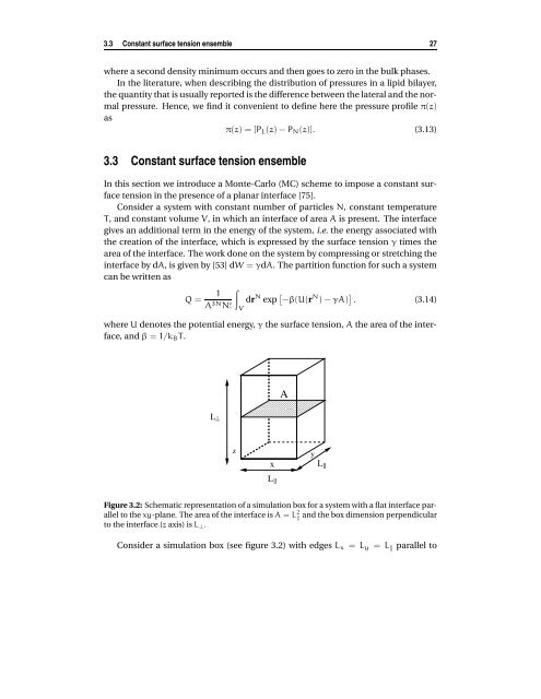
Figure 3.2: Schematic representation of a simulation box for a system with a flat interface parallel
to the xy-plane. The area of the interface is A = L 2
and the box dimension perpendicular
to the interface (z axis) is L⊥.
Consider a simulation box (see figure 3.2) with edges Lx = Ly = L parallel to