The GNSS integer ambiguities: estimation and validation

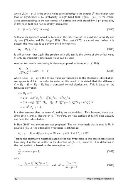
where χ2 α(m−p, 0) is the critical value corresponding to the central χ2-distribution with
level of significance α (= probability in right-hand tail); χ2 β (m − p, δ) is the critical
value corresponding to the non-central χ2-distribution with probability β (= probability
in left-hand tail) and non-centrality parameter:
δ = (ǎ − ǎ2) T G −1
â (ǎ − ǎ2) (3.85)
Still another approach would be to look at the difference of the quadratic forms R1 and
R2, see (Tiberius and De Jonge 1995). First, test (3.76) is carried out. When it is
passed, the next step is to perform the difference test:
R2 − R1 ≥ σ 2 k (3.86)
It will be clear, that again the problem with this test is the choice of the critical value
k, only an empirically determined value can be used.
Another test worth mentioning is the one proposed in Wang et al. (1998):
ˇΩ2 − ˇ Ω
√ ˆσ 2 2 √ δ > tα(m − n − p) (3.87)
where tα(m − n − p) is the critical value corresponding to the Student’s t-distribution,
see appendix A.2.4. In order to arrive at this result it is stated that the difference
d = ˇ Ω2 − ˇ Ω = R2 − R1 has a truncated normal distribution. This is based on the
following derivation:
d = ˇ Ω2 − ˇ Ω
= 2(ǎ − ǎ2) T Q −1
â â + ǎT2 Q −1
â ǎ2 − ǎ T Q −1
â ǎ
= 2(ǎ − ǎ2) T Q −1 T −1
â
Qˆbâ Qâ A Qy y + ǎ T 2 Q −1
â ǎ2 − ǎ T Q −1
â ǎ
= d1A T Q −1
y y + d0
It is then assumed that the terms d1 and d0 are deterministic. This, however, is not true,
since both ǎ and ǎ2 depend on y. Therefore, the test statistic of (3.87) does actually
not have the t-distribution.
In Han (1997) yet another test was proposed. The null hypothesis that is used is H3 in
equation (3.71), the alternative hypothesis is defined as:
Ha : y = Aǎ + A(ǎ2 − ǎ)γ + Bb + e, γ ∈ R, b ∈ R p , e ∈ R m
Testing the alternative hypothesis against the null hypothesis in this case means testing
how likely it is that an outlier in the direction of (ǎ2 − ǎ) occurred. The definition of
the test statistic is based on the assumption that:
γ
ˆσγ
with:
∼ t(m − p − 1) (3.88)
ˆγ = (ǎ2 − ǎ) T G −1
â (â − ǎ)
δ
and ˆσ 2 γ = ˇ Ω − ˆγ 2 δ
m − p − 1
(3.89)
62 Integer ambiguity resolution