The GNSS integer ambiguities: estimation and validation

acceptable. Moreover, the bounds will only be tight if the success rate is high. Furthermore,
it is also interesting to compare the ’quality’ of the float and the fixed baseline
estimators. For that purpose, the probabilities P ( ˇ b ∈ Eb) and P ( ˆ b ∈ Eb) can be considered,
with Eb identical in both cases. But then the choice of the region Eb is not
so straightforward; with equation (3.65) it is not possible to give an exact evaluation of
P ( ˆ b ∈ Eb). Another option is therefore to consider the probabilities:
P ( ˆ b − b 2 Qˆ b ≤ β 2 ) and P ( ˇ b − b 2 Qˇ b ≤ β 2 ) (3.69)
The first probability can be evaluated exactly since ˆb−b2 has a central χ Qˆb 2-distribution. The second probability, however, cannot be evaluated exactly.
Until now the quality of the complete baseline estimator was considered. However, a
user will be mainly interested in the baseline increments, whereas the baseline estimator
may contain other parameters as well, such as ionospheric delays. Therefore, it is more
interesting to look at the probabilities
P ( ˆ bx − bx ≤ β) and P ( ˇ bx − bx ≤ β) (3.70)
where the subscript x is used to indicate that only the baseline parameters referring to
the actual receiver position are considered, i.e. bx = rqr from equation (2.39). So,
ˆ bx − bx is the actual distance to the true receiver position.
Examples
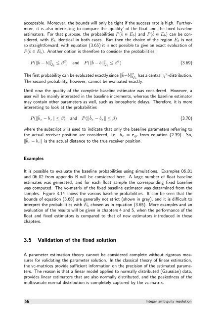
It is possible to evaluate the baseline probabilities using simulations. Examples 06 01
and 06 02 from appendix B will be considered here. A large number of float baseline
estimates was generated, and for each float sample the corresponding fixed baseline
was computed. The vc-matrix of the fixed baseline estimator was determined from the
samples. Figure 3.14 shows the various baseline probabilities. It can be seen that the
bounds of equation (3.68) are generally not strict (shown in grey), and it is difficult to
interpret the probabilities with Eb chosen as in equation (3.65). More examples and an
evaluation of the results will be given in chapters 4 and 5, when the performance of the
float and fixed estimators is compared to that of new estimators introduced in those
chapters.
3.5 Validation of the fixed solution
A parameter estimation theory cannot be considered complete without rigorous measures
for validating the parameter solution. In the classical theory of linear estimation,
the vc-matrices provide sufficient information on the precision of the estimated parameters.
The reason is that a linear model applied to normally distributed (Gaussian) data,
provides linear estimators that are also normally distributed, and the peakedness of the
multivariate normal distribution is completely captured by the vc-matrix.
56 Integer ambiguity resolution