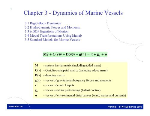
Chapter 3 - Dynamics of Marine Vessels

1
Chapter 3 - Dynamics of Marine Vessels
3.1 Rigid-Body Dynamics
3.2 Hydrodynamic Forces and Moments
3.3 6 DOF Equations of Motion
3.4 Model Transformations Using Matlab
3.5 Standard Models for Marine Vessels
Ṁ C D g g o w
M - system inertia matrix (including added mass)
C - Coriolis-centripetal matrix (including added mass)
D - damping matrix
g - vector of gravitational/buoyancy forces and moments
- vector of control inputs
go - vector used for pretrimming (ballast control)
w - vector of environmental disturbances (wind, waves and currents)
Ivar Ihle – TTK4190 Spring 2006

2
3.2.4 Ballast Systems
A floating or submerged vessel can be pretrimmed by pumping water between the
ballast tanks of the vessel. This implies that the vessel can be trimmed in heave,
pitch and roll:
z zd, d, d 3 modes with restoring forces/moment
Steady-state solution:
where
Ṁ X C X D X g Xgo w
g d g o w
d −, −, −, zd, d, d, −
main equation for ballast computations
The ballast vector g o is computed by using hydrostatic analyses.
Ivar Ihle – TTK4190 Spring 2006

3
3.2.4 Ballast Systems
Consider a marine vessel with n ballast tanks of volumes V i ≤V i,max (i=1,…,n).
For each ballast tank the water volume is defined:
hi
Vihi o
Aihdh ≈ Aihi, (Aih constant)
The gravitational forces W i in heave are:
n n
Zballast ∑ Wi g∑ Vi
i1
i1
h i
A(h)
i i
V i
W i
z
g
x
zoom in
Ivar Ihle – TTK4190 Spring 2006

4
3.2.4 Ballast Systems
Ballast tanks location with respect to O:
Restoring moments due to the heave force Z ballast :
m r f
x
y
z
Resulting
ballast
model:
0
0
Zballast
g o
0
0
Zballast
Kballast
Mballast
0
yZ ballast
−xZballast
0
g
r i b xi, yi, zi , i 1, … , n
0
0
n
∑ Vi i1
n
∑ yi Vi i1
n
−∑ xiVi i1
0
Kballast g∑ i1
Mballast −g∑ i1
Ivar Ihle – TTK4190 Spring 2006
n
n
yiVi
xiVi

5
3.2.4 Ballast Systems
Conditions for Manual Pretrimming
Trimming is usually done under the assumptions that d and d are small such:
Reduced order system (heave, roll, and pitch):
G r
g d ≈ G d
−Zz 0 −Z
0 −K 0
−Mz 0 −M
Steady-state
condition:
−Zz 0 −Z
0 −K 0
−Mz 0 −M
g o r g
G r d r go r w r
zd
d
d
n
∑ Vi i1
n
∑ yiVi i1
n
−∑ xiVi i1
n
g∑ Vi w3
i1
n
g∑ yiVi w4
i1
n
−g∑ xiVi w5
i1
d r zd, d, d
w r w3,w4,w5
This is a set of linear
equations where
the volumes V i
can be found by
assuming that w i =0
(zero disturbances)
Ivar Ihle – TTK4190 Spring 2006

6
3.2.4 Ballast Systems
Assume that the disturbances in heave, roll, and pitch have means of zero.
Consequently:
wr w3, w4, w5 0
and
can be written:
−Zz 0 −Z
0 −K 0
−Mz 0 −M
g
zd
d
d
1 1 1
y1 yn−1 yn −x1 −xn−1 −xn
n
g∑ Vi w3
i1
n
g∑ yiVi w4
i1
n
−g∑ xiVi w5
i1
The water volumes V i is found by using the pseudo-inverse:
H y H HH −1 y
V1
V2
Vn
H y
−Zzzd−Zd
−K d
−Mzzd−Md
Ivar Ihle – TTK4190 Spring 2006

7
3.2.4 Ballast Systems
Example (Semi-Submersible Ballast Control) Consider a semi-submersible
b b b b with 4 ballast tanks located at r1 −x, −y, r2 x, −y, r3 x, y,r4 −x, y
In addition, yz-symmetry implies that Z Mz 0
H g
y
1 1 1 1
−y −y y y
x −x −x x
−Zzzd
−K d
−Md
H y H HH −1 y
V1
V2
V3
V4
1
4g
1 − 1 y
1
x
1 − 1 y − 1 x
1 1 y − 1 x
1 1 y
1
x
gA wp 0z d
g∇GMT d
g∇GML d
gA wp 0z d
g∇GMT d
g∇GML d
p 1
+
V 1
P P
V 4
O
y b
P
P
x b
p 2
Inputs: zd, d, d
+
+
V 2
P P
V 3
p 3
Ivar Ihle – TTK4190 Spring 2006

8
3.2.4 Ballast Systems
SeaLaunch:
An example of a highly sophisticated pretrimming system is the
SeaLaunch trim and heel correction system (THCS):
This system is designed such
that the platform maintains
constant roll and pitch angles
during changes in weight. The
most critical operation is when
the rocket is transported from
the garage on one side of the
platform to the launch pad.
During this operation the
water pumps operate at their
maximum capacity to
counteract the shift in weight.
A feedback system controls the pumps to maintain the
correct water level in each of the legs during
transportation of the rocket
Ivar Ihle – TTK4190 Spring 2006

9
3.2.4 Ballast Systems
Automatic Pretrimming using Feedback from
In the manual pretrimming case it was assumed that wr zd, d, d
=0. This assumption can
be removed by using feedback.
The closed-loop dynamics of a PID-controlled water pump can be described by a
1st-order model with amplitude saturation:
Tjṗ j pj satpdj
T j (s) is a positive time constant
p j (m³/s) is the volumetric flow rate pump j
p d j is the pump set-point.
The water pump capacity is different for
positive and negative flow directions:
satpdj
p j,max pj p j,max
pdj
−
pj,max ≤ pdj ≤ pj,max − −
pj,max pdj pj,max pjmax ,
0.63 pjmax ,
p j
T j
Ivar Ihle – TTK4190 Spring 2006
t

10
3.2.4 Ballast Systems
Example (Semi-Submersible Ballast Control, Continues): The water flow
model corresponding to the figure is:
V̇ 1 −p1
V̇ 2 −p3
V̇ 3 p2 p3
V̇ 4 p1 − p2
Tṗ p satp d
V1
V2
V3
V4
̇ Lp
, p
p1
p2
p3
, L
−1 0 0
0 0 −1
0 1 1
1 −1 0
p 1
+
V 1
P P
V 4
O
y b
P
P
x b
p 2
+
+
V 2
P P
V 3
p 3
Ivar Ihle – TTK4190 Spring 2006

11
3.2.4 Ballast Systems
Feedback control system:
p d HpidsG r d r − r
Hpids diagh1,pids, h2,pids,...,hm,pids
ballast
controller
G r
r
ηd -
p d
sat( . )
-
T -1
Closed-loop pump dynamics with water volume as output
Dynamics:
p
Tṗ p satp d
̇ Lp
L
υ
r go ( υ)
( G )
r -1
Steady-state relationship for
water volume and trim
G r r g o r w r
η r
Equilibrium equation:
Ivar Ihle – TTK4190 Spring 2006

12
3.2.4 Ballast Systems
SeaLaunch Trim and Heel Correction System (THCS)
(Courtesy: Sea Launch LDC)
Ivar Ihle – TTK4190 Spring 2006

13
3.2.4 Ballast Systems
Ivar Ihle – TTK4190 Spring 2006

14
Pitch angle (deg)
3.2.4 Ballast Systems
Roll and pitch angles during lift-off
roll
roll and pitch (deg)
pitch
4.21
A 1 < > jp
0.95
5.5 6
4.5 5
3.5 4
2.5 3
1.5 2
0.5 1
0.5 0
1.5 1
6
4
2
0
2
0 187.5 375 562.5 750 937.5 1125 1312.5 1500
2
420 430 440 450 460 470
420 jp
time (secs)
Measured pitch during launch
Roll and pitch during launch
470
pitch angle (deg)
4.326
Z 4 < > . 180
l
π
0.202
6
4
2
0
2
time (secs)
20 10 0 10 20 30
15
Z
time (secs)
1 < > l
Calculated pitch motions
29.775
Ivar Ihle – TTK4190 Spring 2006

15
3.3 6 DOF Equations of Motion
Body-Fixed Vector Representation
M ̇ C D g g o w
̇ J
M MRB MA
C CRB CA
D DP DS DW DM
NED Vector Representation
Kinematic transformation (assuming that J exists-i.e., ):
−1 ≠ /2
̇ J J−1 ̇
̈ J ̇ ̇J ̇ J−1̈ − ̇JJ −1 ̇
M ∗ J − M J −1
C ∗ , J − C − MJ −1 ̇JJ −1
D∗, J− D J−1 g∗ J− g
M ∗ ̈ C ∗ , ̇ D ∗ , ̇ g ∗ J − g o w
Ivar Ihle – TTK4190 Spring 2006

16
3.3.1 Nonlinear Equations of Motion
Properties of the NED Vector Representation
M ∗ ̈ C ∗ , ̇ D ∗ , ̇ g ∗ J − g o w
(1) M ∗ M ∗ 0 ∀ ∈ 6
(2) s ̇ M ∗ − 2C ∗ , s 0 ∀ s ∈ 6 , ∈ 6 , ∈ 6
(3) D ∗ , 0 ∀ ∈ 6 , ∈ 6
if M M 0and ̇ M 0.
It should be noted that C ∗ , will not be skew-symmetrical although C is skew-symmetrical.
Ivar Ihle – TTK4190 Spring 2006

17
3.3.1 Nonlinear Equations of Motion
Property (System Inertia Matrix) For a rigid body the system inertia matrix is
strictly positive if and only if M A >0, that is:
If the body is at rest (or at most is moving at low speed) under the assumption of
an ideal fluid, the zero-frequency system inertia matrix is always positive definite,
that is
M M 0
where:
M
M MRB MA 0
m − Xu̇ −Xv̇ −Xẇ
−Xv̇ m − Yv̇ −Yẇ
−Xẇ −Yẇ m − Zẇ
−Xṗ −mzg−Yṗ my g −Zṗ
mzg−Xq̇ −Yq̇ −mxg−Zq̇
−my g −Xṙ mxg−Yṙ −Zṙ
M ≠ M
−Xṗ mzg−Xq̇ −my g −Xṙ
−mzg−Yṗ −Yq̇ mxg−Yṙ
my g −Zṗ −mxg−Zq̇ −Zṙ
Ix−Kṗ −Ixy−Kq̇ −Izx−Kṙ
−Ixy−Kq̇ Iy−Mq̇ −Iyz−Mṙ
−Izx−Kṙ −Iyz−Mṙ Iz−Nṙ
Ivar Ihle – TTK4190 Spring 2006

18
3.3.1 Nonlinear Equations of Motion
Property (Coriolis and Centripetal Matrix): For a rigid body moving
through an ideal fluid the Coriolis and centripetal matrix can always be
parameterized such that it is skew-symmetric, that is
If M is nonsymmetric, we write M as the sum of a symmetric and skewsymmetric
matrix:
where
C −C , ∀ ∈ 6
M 1
2 M M 1
2 M − M
M 0 T 1
2 M 1
2 M̄ 0
M̄ M̄ 1
2 M M 0
This implies that we can compute C from
M̄ M̄ 0
1
2 M − M 0
Ivar Ihle – TTK4190 Spring 2006

19
3.3.2 Linearized Equations of Motion
Assumption (Small Roll and Pitch Angles) The roll and pitch angles:
These are good assumptions for vessels where the pitch and roll motions are
limited-i.e., highly metacentric stable vessels
This assumption implies that:
where
, are small
̇ J 0
≈ P
P
R 033
033 I33
Ivar Ihle – TTK4190 Spring 2006

20
3.3.2 Linearized Equations of Motion
Definition (Vessel Parallel Coordinate System) The vessel parallel coordinate
system is defined as:
where p is the NED position/attitude decomposed in body coordinates and P
is given by
Notice that P T P = I 6×6 .
NED
y n
xn
p P
P
R 033
033 I33
p
BODY
y b
x b
Ivar Ihle – TTK4190 Spring 2006

21
3.3.2 Linearized Equations of Motion
Low Speed Applications (Station-Keeping)
Vessel parallel (VP) coordinates implies:
̇ p Ṗ P ̇
Ṗ P p P P
rS p
where and
r ̇
S
0 1 0 0 0 0
−1 0 0 0 0 0
0 0 0 0 0 0
0 0 0 0 0 0
0 0 0 0 0 0
For low speed applications r ≈ 0. This gives a linear model:
̇ p ≈
Ivar Ihle – TTK4190 Spring 2006

22
3.3.2 Linearized Equations of Motion
The gravitational and buoyancy forces can also be expressed in terms of VP
coordinates. For small roll and pitch angles:
g
Notice that this formula confirms that the restoring forces of a leveled vessel
( ) is independent of the yaw angle .
0
≈ PG PGP p Gp G
0
For a neutrally buoyant submersible (W=B) with x g =x b and y g =y b we have:
G diag0, 0, 0, 0, zg − zbW, zg − zbW,0
For a surface vessel G is defined as:
G
022
032
023
G r
0 0 0 0 0 0
0
0
0
0
, G r
−Zz 0 −Z
0 −K 0
−Mz 0 −M
P Notice that:
GP ≡ G
Ivar Ihle – TTK4190 Spring 2006

23
3.3.2 Linearized Equations of Motion
Low-Speed Maneuvering and DP: ≈ 0 implies that the nonlinear Coriolis,
centripetal, damping, restoring, and buoyancy forces and moments can be
linearized about 0 and 0.
Since C(0)=0 and Dn (0)=0 it makes
sense to: approximate:
Ṁ C D Dn
0
D
The resulting state-space model becomes:
A
̇ p
Ṁ D G p w
0 I
−M−1G −M−1D P p
, B
g Gp
0
M−1 g o w
̇x Ax Bu Ew
x p , , u
, E
0
M−1 which is the linear time invariant (LTI) state-space model used in DP.
Ivar Ihle – TTK4190 Spring 2006

24
3.3.2 Linearized Equations of Motion
Vessels in Transit (Cruise Condition):
For vessels in transit the cruise speed is assumed to satisfy:
u uo
This suggests that
where
o uo,0,0,0,0,0
Nuo ∂
∂ C D| o
̇ p Δ o
MΔ̇ NuoΔ G p w
Linear parameter varying (LPV) model:
Auo
̇x Auox Bu Ew Fo
0 I
−M−1G −M−1Nuo , B
0
M−1 , E
0
M−1 Δ − o
x p ,Δ
, F
I
0
Ivar Ihle – TTK4190 Spring 2006

25
3.5 Standard Models for Marine Vessels
Models for ships, semi-submersibles, and underwater vehicles are usually
represented as one of the following subsystemes:
or:
Surge model: velocity u
Maneuvering model (sway and yaw): velocities v and r
Horizontal motion (surge, sway, and yaw): velocities u,v, and r
Longitudinal motion (surge, heave, and pitch): velocities u,w, and q
Lateral motion: (sway, roll, and yaw): velocities v,p, and r
Horizontal plane models: DOFs 1, 2, 6
Longitudinal motion: DOFs 1, 3, 5
Lateral motion: DOFs 2, 4, 6
Ivar Ihle – TTK4190 Spring 2006

26
3.5.1 3 DOF Horizontal Motion
The horizontal motion of a ship or
semi-submersible is described by
the motion components in surge,
sway, and yaw.
u, v, r n,e,
This implies that the dynamics
associated with the motion in heave,
roll, and pitch are neglected, that is
w=p=q=0.
Low-speed applications-i.e., dynamically positioned ships where U≈0,
and maneuvering at high speed will now be treated separately.
Ivar Ihle – TTK4190 Spring 2006

27
3.5.1 3 DOF Horizontal Motion
Low-Speed Model for Dynamically Positioned Ship
Consider the 6 DOF kinematic expressions:
J
R b n Θ
TΘΘ
R b n Θ 033
033 TΘΘ
cc −sc css ss ccs
sc cc sss −cs ssc
−s cs cc
1 st ct
0 c −s
0 s/c c/c
For small roll and pitch angles and no heave this reduces to:
J
3 DOF
R
cos − sin 0
sin cos 0
0 0 1
Ivar Ihle – TTK4190 Spring 2006

28
3.5.1 3 DOF Horizontal Motion
Assume that the ship has homogeneous mass distribution, xz-plane symmetry and y g =0:
MRB
MA −
m 0 0 0 mzg −my g
0 m 0 −mzg 0 mxg
0 0 m my g −mxg 0
0 −mzg my g Ix −Ixy −Ixz
mzg 0 −mxg −Iyx Iy −Iyz
X
−my g mxg 0 −Izx −Izy Iz
Xu̇ Xv̇ Xẇ Xṗ Xq̇ Xṙ
X
Yu̇ Yv̇ Yẇ Yṗ Yq̇ Yṙ
Zu̇ Zv̇ Zẇ Zṗ Zq̇ Zṙ
Ku̇ Kv̇ Kẇ Kṗ Kq̇ Kṙ
Mu̇ Mv̇ Mẇ Mṗ Mq̇ Mṙ
X
X
X
Nu̇ Nv̇ Nẇ Nṗ Nq̇ Nṙ
X
MRB
CRB
MA
CA
m 0 0
0 m mxg
0 mxg Iz
0 0 −mx g r v
0 0 mu
mx g r v −mu 0
−Xu̇ 0 0
0 −Y v̇ −Y ṙ
0 −Yṙ −Nṙ
0 0 Y v̇ v Y ṙ r
0 0 −Xu̇ u
−Yv̇ v − Y ṙ r Xu̇ u 0
Ivar Ihle – TTK4190 Spring 2006

29
3.5.1 3 DOF Horizontal Motion
For the 3 DOF low speed model, M = M T and C = -C T , that is:
M
C
m − Xu̇ 0 0
0 m − Yv̇ mxg−Y ṙ
0 mxg−Y ṙ Iz−Nṙ
As for the system inertia matrix, linear damping in surge is decoupled from sway
and yaw. This implies that:
D
0 0 − m − Y v̇ v − mx g −Yṙ r
0 0 m − X u̇ u
m − Y v̇ v mx g −Y ṙ r −m − X u̇ u 0
−Xu 0 0
0 −Yv −Y r
0 −Nv −Nr
Linear damping is a good assumption for low-speed applications. Similarly the
quadratic velocity terms given by C
are negligible in DP
Ivar Ihle – TTK4190 Spring 2006

30
3.5.1 3 DOF Horizontal Motion
Resulting Low-Speed (DP) Model:
̇ R
Ṁ D
where
Bu
M = M
B is the control matrix describing the thruster configuration and u is the control input.
T >0 and D = DT >0
Nonlinear Maneuvering Model:
At higher speeds the assumptions that D D Dn≈ D and C≈ 0 are violated
This suggests the following 3 DOF nonlinear maneuvering model:
̇ R
Ṁ C D
Ivar Ihle – TTK4190 Spring 2006

31
3.5.2 Decoupled Models for Forward
Speed/Maneuvering
For vessels moving at constant (or at least slowly-varying) forward speed:
U u 2 v 2 ≈ u
the 3 DOF maneuvering model can be decoupled in a:
Forward speed (surge subsystem)
Sway-yaw subsystem for maneuvering
Forward Speed Model
Starboard-port symmetry implies that surge is decoupled from sway and yaw:
m − Xu̇ u̇ − Xuu − X|u|u|u|u 1
where 1
is the sum of control forces in surge. Notice that both linear and quadratic
damping have been included in order to cover low- and high-speed applications.
Ivar Ihle – TTK4190 Spring 2006

32
3.5.2 Decoupled Models for Forward
Speed/Maneuvering
2 DOF Linear Maneuvering Model (Sway-Yaw Subsystem)
A linear maneuvering model is based on the assumption that the cruise speed:
u uo ≈ constant
while v and r are assumed to be small.
Representation 1 (see also lecture notes by Professor David Clark)
The 2nd and 3rd rows in the DP model
with u=u o , yields:
C
C
0 0 − m − Y v̇ v − mx g −Yṙ r
0 0 m − X u̇ u
m − Y v̇ v mx g −Y ṙ r −m − X u̇ u 0
m − X u̇ u o r
m − Y v̇ u o v mx g −Y ṙ u o r − m − X u̇ u o v
0 m − X u̇ u o
X u̇ −Yv̇ u o mx g −Y ṙ u o
v
r
Notice that
C ≠−C
Ivar Ihle – TTK4190 Spring 2006

33
3.5.2 Decoupled Models for Forward
Speed/Maneuvering
Assume that the ship is controlled by a single rudder:
and that linear damping dominates:
then:
where
v, r
b
−Y
−N
D D D n ≈ D
Ṁ Nuo b
This is the linear maneuvering model
as used by Clark, Fossen and others.
Developed from M RB , C RB , M A , C A
Notice: N includes the famous
Munk moment and some other C A -terms
M
Nuo
b
m − Yv̇ mxg−Yṙ
mxg−Y ṙ
−Yv
Iz−Nṙ
m − X u̇ u o −Yr
X u̇ −Yv̇ u o −Nv mx g −Y ṙ u o −Nr
−Y
−N
Ivar Ihle – TTK4190 Spring 2006

34
3.5.2 Decoupled Models for Forward
Speed/Maneuvering
2 DOF Linear Maneuvering Model (Sway-Yaw Subsystem)
Representation 2 (Davidson and Schiff 1946). Starts with Newton’s law:
where linear terms in acceleration, velocity and rudder are added according to:
Notice: This approach does not included the C A -matrix. The resulting model is:
M
MRḂ CRB RB
RB −
Y
N
m − Yv̇ mxg−Yṙ
mxg−Y ṙ
Iz−Nṙ
Yv̇ Yṙ
Nv̇ Nṙ
Ṁ Nuo b
, Nuo
In this model the Munk moment is missing in the yaw equation. This is a destabilizing moment
known from aerodynamics which tries to turn the vessel. Also notice that two other less
important C A -terms are removed from N(u o ) when compared to Representation 1.
̇
−Yv
Yv Yr
Nv Nr
muo−Y r
−Nv mxguo−Nr
, b
−Y
−N
Ivar Ihle – TTK4190 Spring 2006

35
3.5.2 Decoupled Models for Forward
Speed/Maneuvering
1 DOF Autopilot Model (Yaw Subsystem)
A linear autopilot model for course control can be derived from the maneuvering model
Ṁ Nuo b
by defining the yaw rate r as output:
r c , c 0, 1
Hence, application of the Laplace transformation yields (Nomoto 1957):
r
s
The 1st-order Nomoto model is obtained by defining the equivalent time constant as:
T T1 T2 − T3
r
s K
1Ts
K1T3s
1T1s1T2s
2nd-order Nomoto model
̇ r
s K
s1Ts
Ivar Ihle – TTK4190 Spring 2006

36
3.5.3 Longitudinal and Lateral Models
The 6 DOF equations of motion can in many cases be divided into two noninteracting
(or lightly interacting) subsystems:
Longitudinal subsystem: states u,w,q, and
Lateral subsystem: states v,p,r, and
This decomposition is good for slender bodies (large length/width ratio). Typical
applications are aircraft, missiles, and submarines.
Ivar Ihle – TTK4190 Spring 2006

37
3.5.3 Longitudinal and Lateral Models
M
M
m11 m12 0 0 0 m16
m21 m22 0 0 0 m26
0 0 m33 m34 m35 0
0 0 m43 m44 m45 0
0 0 m53 m54 m55 0
m61 m62 0 0 0 m66
xy-plane of symmetry
(bottom/top symmetry):
m11 0 0 0 m15 0
0 m22 0 m24 0 0
0 0 m33 0 0 0
0 m42 0 m44 0 0
m51 0 0 0 m55 0
0 0 0 0 0 m66
yz-plane of symmetry
(fore/aft symmetry)
M
m11 0 m13 0 m15 0
0 m22 0 m24 0 m26
m31 0 m33 0 m35 0
0 m42 0 m44 0 m46
m51 0 m53 0 m55 0
0 m62 0 m64 0 m66
xz-plane of symmetry
(port/starboard symmetry)
M diagm11,m 22,m 33,m 44,m 55,m 66
xz-, yz- and xy-planes of symmetry
(port/starboard, fore/aft and bottom/top
symmetries).
Ivar Ihle – TTK4190 Spring 2006

38
3.5.3 Longitudinal and Lateral Models
Starboard-port symmetry implies the following zero elements:
M
m11 0 m13 0 m15 0
0 m22 0 m24 0 m26
m31 0 m33 0 m35 0
0 m42 0 m44 0 m46
m51 0 m53 0 m55 0
0 m62 0 m64 0 m66
The longitudinal and lateral submatrices are:
M long
m11 m13 m15
m31 m33 m35
m51 m53 m55
, M lat
m22 m24 m26
m42 m44 m46
m62 m64 m66
Ivar Ihle – TTK4190 Spring 2006

39
3.5.3 Longitudinal and Lateral Models
Longitudinal Subsystem (DOFs 1, 3, 5)
J
R b n Θ
TΘΘ
R b n Θ 033
033 TΘΘ
cc −sc css ss ccs
sc cc sss −cs ssc
−s cs cc
1 st ct
0 c −s
0 s/c c/c
Resulting kinematic equation:
ḋ ̇
cos 0
0 1
v, p, r, are small
w
q
− sin
0
not controlling the N-position
using speed control instead
u
Ivar Ihle – TTK4190 Spring 2006

40
3.5.3 Longitudinal and Lateral Models
Longitudinal Subsystem (DOFs 1, 3, 5)
For simplicity, it is assumed that higher order damping can be neglected, that is
Dn 0. Coriolis is, however, modelled by assuming that u 0 and that
2nd-order terms in v,w,p,q, and r are small. Hence, DOFs 1, 3, 5 gives:
CRB
CRB ≈
my g q z g rp − mx g q − wq − mx g r vr
−mz g p − vp − mz g q uq mx g p y g qr
mx g q − wu − mz g r xgpv mz g q uw I yz q I xz p − I z rp −I xz r − Ixyq I x pr
Collecting terms in u,w, and q, gives:
0 0 0
0 0 −mu
0 0 mxgu
Assuming a diagonal M A gives:
CA
−Zẇ wq Y v̇ vr
−Y v̇ vp X u̇ uq
u
w
Z ẇ −Xu̇ uw N ṙ −Kṗ pr
q
≈
0 0 0
0 0 Xu̇ u
0 Z ẇ −Xu̇ u 0
CRB ≠−CRB
The skew-symmetric property is
destroyed for the decoupled model:
u
w
q
Ivar Ihle – TTK4190 Spring 2006

41
3.5.3 Longitudinal and Lateral Models
Longitudinal Subsystem (DOFs 1, 3, 5)
The restoring forces with W=B and xg =xb :
g
g
−
W − B sin
W − B cos sin
− W − B cos cos
− ygW − ybB cos cos zgW − zbB cos sin
z g W − zbB sin x g W − xbB cos cos
− x g W − xbB cos sin − y g W − y b B sin
0
0
WBGz sin
Ivar Ihle – TTK4190 Spring 2006

42
3.5.3 Longitudinal and Lateral Models
Longitudinal Subsystem (DOFs 1, 3, 5)
m − Xu̇ −Xẇ mzg − Xq̇
−Xẇ m − Zẇ −mxg − Zq̇
mzg − Xq̇ −mxg − Zq̇ Iy − Mq̇
0 0 0
0 0 −m − Xu̇ u
0 Zẇ − Xu̇ u mxgu
u uo constant
m − Zẇ
−mxg−Zq̇
−mxg−Zq̇
Iy−Mq̇
0 −m − X u̇ u o
Z ẇ −Xu̇ u o
mxguo
ẇ
q̇
w
q
u
w
q
u̇
ẇ
q̇
−Zw −Zq
−Mw −Mq
−Xu −Xw −Xq
−Zu −Zw −Zq
−Mu −Mw −Mq
0
0
WBGz sin
0
BGzWsin
w
q
3
5
1
3
5
u
w
q
Ivar Ihle – TTK4190 Spring 2006

43
3.5.3 Longitudinal and Lateral Models
Longitudinal Subsystem (DOFs 1, 3, 5)
Linear pitch dynamics (decoupled):
where the natural frequency is:
Iy − Mq̇ ̈ − Mq̇ BGzW 5
BGz W
Iy−Mq̇
Ivar Ihle – TTK4190 Spring 2006

44
3.5.3 Longitudinal and Lateral Models
Lateral Subsystem (DOFs 2, 4, 6)
J
R b n Θ
TΘΘ
R b n Θ 033
033 TΘΘ
cc −sc css ss ccs
sc cc sss −cs ssc
−s cs cc
1 st ct
0 c −s
0 s/c c/c
Resulting kinematic equation:
̇ p
̇ r
u, w, p, r, and are small
not controlling the E-position
using heading control instead
Ivar Ihle – TTK4190 Spring 2006

45
3.5.3 Longitudinal and Lateral Models
Lateral Subsystem (DOFs 2, 4, 6)
Again it is assumed that higher order velocity terms can be neglected so that
Dn 0.
Hence:
CRB
Collecting terms in v,p, and r, gives:
CRB ≈
Assuming a diagonal M A gives:
CA
−my g p wp mz g r xgpq − my g r − ur
−my g q z g ru my g p wv mz g p − vw −I yz q − I xz p I z rq I yz r Ixyp − I y qr
mx g r vu my g r − uv − mx g p y g qw −I yz r − Ixyp I y qp I xz r Ixyq − I x pq
0 0 muo
0 0 0
0 0 mxguo
Zẇ wp − X u̇ ur
Y v̇ −Zẇ vw M q̇ −Nṙ qr
X u̇ −Y v̇ uv K ṗ −Mq̇ pq
v
p
r
≈
CRB ≠−CRB
The skew-symmetric property is
destroyed for the decoupled model:
0 0 −Xu̇ u
0 0 0
X u̇ −Y v̇ u 0 0
v
p
r
Ivar Ihle – TTK4190 Spring 2006

46
3.5.3 Longitudinal and Lateral Models
Lateral Subsystem (DOFs 2, 4, 6)
The restoring forces with W=B, xg =xb and yg =zg :
g
g
−
W − B sin
W − B cos sin
− W − B cos cos
− ygW − ybB cos cos zgW − zbB cos sin
z g W − zbB sin x g W − xbB cos cos
− x g W − xbB cos sin − y g W − y b B sin
0
WBGzsin 0
Ivar Ihle – TTK4190 Spring 2006

47
3.5.3 Longitudinal and Lateral Models
Lateral Subsystem (DOFs 2, 4, 6)
m − Yv̇ −mzg − Yṗ mxg − Yṙ
−mzg − Yṗ Ix − Kṗ −Izx − Kṙ
mxg − Yṙ −Izx − Kṙ Iz − Nṙ
0 0 m − Xu̇ u
0 0 0
Xu̇ − Yv̇ u 0 mxgu
u uo constant
m − Yv̇ mxg−Yṙ
mxg−Y ṙ
Iz−Nṙ
v̇
ṙ
0 m − X u̇ u o
X u̇ −Y v̇ u o
mxguo
v
p
r
v̇
ṗ
ṙ
−Yv −Yr
−Nv −Nr
v
r
−Yv −Yp −Yr
−Mv −Mp −Mr
−Nv −Np −Nr
0
WBGzsin 0
v
r
2
6
2
4
6
v
p
r
Ivar Ihle – TTK4190 Spring 2006

48
3.5.3 Longitudinal and Lateral Models
Lateral Subsystem (DOFs 2, 4, 6)
Linear roll dynamics (decoupled):
where the natural frequency is:
Ix − Kṗ ̈ − Kp ̇ WBGz 4
BGz W
Ix−Kṗ
Ivar Ihle – TTK4190 Spring 2006