Rasmus ÿstergaard forside 100%.indd - Solid Mechanics

Interface crack in sandwich specimen 305
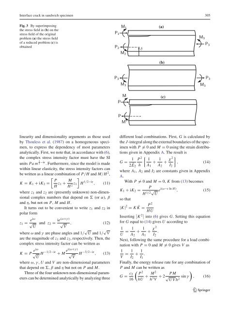
Fig. 3 By superimposing
the stress field in (b) onthe
stress field of the original
problem (a) the stress field
of a reduced problem (c) is
obtained
linearity and dimensionality arguments as those used
by Thouless et al. (1987) on a homogeneous specimen,
to express the dependency of most parameters
analytically. First, we note that, in accordance with (6),
the complex stress intensity factor must have the SI
units Pa m 1 2 −iɛ . Furthermore, since the model is made
within linear elasticity, the stress intensity factors can
be written as a linear combination of P/H and M/H 2 ,
P
K = K1 + iK2 =
H z1 + M
z1 H
H 2 1/2−iɛ , (11)
where z1 and z2 are (presently unknown) non-dimensional
complex numbers that depend on (or α), β
and η, but not on P, M and H.
It turns out to be convenient to write z1 and z2 in
polar form
z1 = eiω
√ U and z2 = ie(ω+γ)
√ V , (12)
where ω and γ are phase angles and 1/ √ U and 1/ √ V
are the magnitude of z1 and z2, respectively. Then, the
complex stress intensity factor can be written as
K = P eiω
√ U H −1/2−iɛ + M ei(ω+γ)
√ V H −3/2−iɛ , (13)
where ω, γ , U and V are non-dimensional parameters
that depend on , β and η but not on P and M.
Three of the four unknown non-dimensional parameters
can be determined analytically by analyzing three
P1
M1
P2
M2
P3
M3
M3 M3
M
P
P
M∗ δ
(a)
(b)
(c)
different load combinations. First, G is calculated by
the J-integral along the external boundaries of the specimen
with P = 0 and M = 0 using the strain distributions
given in Appendix A. The result is
G = 1 P
2Ē2
2
1
+
h A1
1
+
A2
χ 2
, (14)
I2
where A1, A2 and I2 are constants given in Appendix
A.
With P = 0 and M = 0, K from (13) becomes
P
K1 + iK2 =
H 1/2√U ei(ω−ɛ ln H) , (15)
so that
|K | 2 = K ¯K = P2
HU
Inserting K 2 into (6) givesG. Setting this equation
for G equal to (14) givesUaccording to
1 1
= +
U A2
1
+
A1
χ 2
.
I2
Next, following the same procedure for a load combination
with P = 0 and M = 0givesVas 1 1
= +
V I2
1
.
I1
Finally, the energy release rate for any combination of
P and M can be written as
G = c2
P2 M2
+
16 hU h3
PM
+ 2√ sin γ , (16)
V UVh2 P3
P3
123