Dynamics of Machines - Part II - IFS.pdf
Dynamics of Machines - Part II - IFS.pdf Dynamics of Machines - Part II - IFS.pdf
1.8.5 Experimental – Natural Frequencies (a) Amplitude [m/s 2 ] (b) Amplitude [m/s 2 ] 2 1 0 −1 −2 x Signal 10−4 3 1 (a) in Time Domain − (b) in Frequency Domain 0 5 10 15 time [s] 20 25 30 x 10−5 2 0 0 5 10 15 20 25 frequency [Hz] Figure 34: Transient Vibration – Acceleration of the clamped-free flexible beam when two concentrated masses m = m1 + m2 = 0.382 Kg are attached at its free end (L3 = 0.610 m), two additional masses m = m1 + m2 = 0.382 Kg are attached at its length (L2 = 0.410 m) and two additional masses m = m1 +m2 = 0.382 Kg are attached at its length (L1 = 0.210 m) – Natural frequencies of the 3 D.O.F. mass-spring system ”A”: 1.03 Hz, 7.00 Hz and 19.31 Hz. 1.8.6 Experimental – Resonances and Mode Shapes • Visualization of the participation of modes shapes in the transient response – Visualization using your eyes! Transient motion of the physical system excited with different initial conditions by using your fingers! • Applying an oscillatory excitation by using your finger at the 3 different points of the physical system (co-ordinates of the mechanical model) and detecting the participation of the mode shapes in the permanent solution or steady-state response by using your eyes. 56
(a) Amplitude [m/s 2 ] (b) Amplitude [m/s 2 ] (a) Amplitude [m/s 2 ] (b) Amplitude [m/s 2 ] (a) Amplitude [m/s 2 ] (b) Amplitude [m/s 2 ] 2 1 0 −1 −2 x 10 −5 Signal (a) in Time Domain − (b) in Frequency Domain 0 5 10 15 time [s] 20 25 30 1.5 1 0.5 x 10 −5 0 0 5 10 15 20 25 frequency [Hz] 2 1 0 −1 −2 1.5 0.5 x 10 −5 Signal (a) in Time Domain − (b) in Frequency Domain 0 5 10 15 time [s] 20 25 30 1 x 10 −5 0 0 5 10 15 20 25 frequency [Hz] 2 1 0 −1 −2 1.5 0.5 x 10 −5 Signal (a) in Time Domain − (b) in Frequency Domain 0 5 10 15 time [s] 20 25 30 1 x 10 −5 0 0 5 10 15 20 25 frequency [Hz] Figure 35: Resonance phenomena due to the excitation force with frequencies around the natural frequencies of the mass-spring system: 3 D.O.F. system with the natural frequencies of 0.75 Hz, 5.12 Hz and 14.68 Hz, excited by the shaker – Spring-mass system ”A” with two masses m = m1 + m2 = 0.382 Kg fixed at the beam length L3 = 0.610 m, two additional masses fixed at L2 = 0.410 m and two more at L1 = 0.210 m. 57
- Page 5 and 6: 1.3 Data of the Mechanical System
- Page 7 and 8: 1.5 Calculating Stiffness Matrices
- Page 9 and 10: 1.6 Mechanical Systems with 1 D.O.F
- Page 11 and 12: Demanding (λ 2 + 2ξωnλ + ω 2 n
- Page 13 and 14: 1 yini − A det λ1 vini − A C2
- Page 15 and 16: 1.6.4 Analytical and Numerical Solu
- Page 17 and 18: (a) y(t) [m] (b) y(t) [m] (c) y(t)
- Page 19 and 20: 1.6.6 Homogeneous Solution or Free-
- Page 21 and 22: (a) Amplitude [m/s 2 ] x Signal 10
- Page 23 and 24: (a) Amplitude [m/s 2 ] (b) Amplitud
- Page 25 and 26: Imag(A(ω)) [m/N] 0 −1 −2 −3
- Page 27 and 28: 1.6.11 Superposition of Transient a
- Page 29 and 30: (a) Amplitude [m/s 2 ] (b) Amplitud
- Page 31 and 32: 1.7 Mechanical Systems with 2 D.O.F
- Page 33 and 34: ⎧ ⎫ ⎪⎨ ˙y1(t) ⎪⎬ ˙y
- Page 35 and 36: zini = U c + A ⇒ c = U −1 {(zin
- Page 37 and 38: 1.7.4 Modal Analysis using Matlab e
- Page 39 and 40: 0.7 0.6 0.5 0.4 0.3 0.2 0.1 First M
- Page 41 and 42: %__________________________________
- Page 43 and 44: ||y 1 (ω)|| [m/N] Phase [ o] Excit
- Page 45 and 46: ||y i (ω)|| [m/N] Phase [ o] 0.8 0
- Page 47 and 48: Imag(y i (ω)/f 1 (ω)) (i=1,2) [m/
- Page 49 and 50: 1.8 Mechanical Systems with 3 D.O.F
- Page 51 and 52: which could be verified using Modal
- Page 53 and 54: %%%%%%%%%%%%%%%%%%%%%%%%%%%%%%%%%%%
- Page 55: 1.8.4 Theoretical Frequency Respons
- Page 59 and 60: 4. Vary the number of masses attach
- Page 61 and 62: 1.10 Project 0 - Identification of
- Page 63 and 64: (a) (b) REAL(Acc/force) [(m/s 2 )/N
- Page 65 and 66: 6. Model application - As explained
- Page 67 and 68: changeable unbalanced mass for simu
- Page 69 and 70: %Modal Matrix u with mode shapes %M
- Page 71 and 72: acc [m/s 2 ] acc [m/s 2 ] 0.8 0.6 0
1.8.5 Experimental – Natural Frequencies<br />
(a) Amplitude [m/s 2 ]<br />
(b) Amplitude [m/s 2 ]<br />
2<br />
1<br />
0<br />
−1<br />
−2<br />
x Signal 10−4<br />
3<br />
1<br />
(a) in Time Domain − (b) in Frequency Domain<br />
0 5 10 15<br />
time [s]<br />
20 25 30<br />
x 10−5<br />
2<br />
0<br />
0 5 10 15 20 25<br />
frequency [Hz]<br />
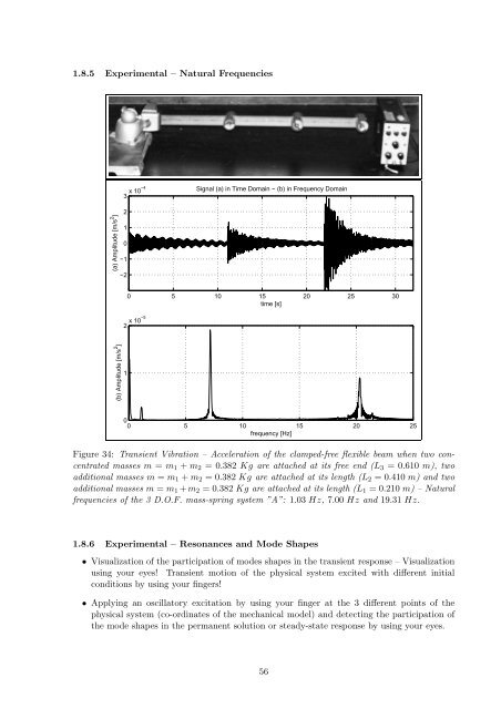
Figure 34: Transient Vibration – Acceleration <strong>of</strong> the clamped-free flexible beam when two concentrated<br />
masses m = m1 + m2 = 0.382 Kg are attached at its free end (L3 = 0.610 m), two<br />
additional masses m = m1 + m2 = 0.382 Kg are attached at its length (L2 = 0.410 m) and two<br />
additional masses m = m1 +m2 = 0.382 Kg are attached at its length (L1 = 0.210 m) – Natural<br />
frequencies <strong>of</strong> the 3 D.O.F. mass-spring system ”A”: 1.03 Hz, 7.00 Hz and 19.31 Hz.<br />
1.8.6 Experimental – Resonances and Mode Shapes<br />
• Visualization <strong>of</strong> the participation <strong>of</strong> modes shapes in the transient response – Visualization<br />
using your eyes! Transient motion <strong>of</strong> the physical system excited with different initial<br />
conditions by using your fingers!<br />
• Applying an oscillatory excitation by using your finger at the 3 different points <strong>of</strong> the<br />
physical system (co-ordinates <strong>of</strong> the mechanical model) and detecting the participation <strong>of</strong><br />
the mode shapes in the permanent solution or steady-state response by using your eyes.<br />
56


