Dynamics of Machines - Part II - IFS.pdf
Dynamics of Machines - Part II - IFS.pdf Dynamics of Machines - Part II - IFS.pdf
1.7.9 Resonance – Experimental Analysis in Time Domain (a) Amplitude [m/s 2 ] 1 0 −1 x Signal 10−5 2 (a) in Time Domain − (b) in Frequency Domain −2 0 5 10 15 time [s] 20 25 30 (b) Amplitude [m/s 2 ] 4 3 2 1 x 10 −6 0 0 5 10 15 20 25 frequency [Hz] (a) Amplitude [m/s 2 ] 1 0 −1 x Signal 10−5 2 (a) in Time Domain − (b) in Frequency Domain −2 0 5 10 15 time [s] 20 25 30 (b) Amplitude [m/s 2 ] 8 6 4 2 x 10 −6 0 0 5 10 15 20 25 frequency [Hz] Figure 31: Resonance phenomena due to the excitation force with frequency around the natural frequency of the mass-spring system: 2 D.O.F. system with the natural frequencies of 0.62 Hz and 4.59, excited by the shaker – Spring-mass system ”A” with three masses m = m1+m2+m3 = 0.573 Kg fixed at the beam length L2 = 0.610 m and three additional masses m = m4+m5+m6 = 0.573 Kg fixed at the middle L1 = 0.310 m resulting in two natural frequencies of 0.62 Hz and 4.60 Hz. 48
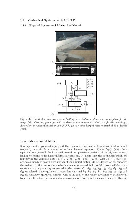
1.8 Mechanical Systems with 3 D.O.F. 1.8.1 Physical System and Mechanical Model (a) (b) (c) Figure 32: (a) Real mechanical system built by three turbines attached to an airplane flexible wing; (b) Laboratory prototype built by three lumped masses attached to a flexible beam); (c) Equivalent mechanical model with 3 D.O.F. for the three lumped masses attached to a flexible beam. 1.8.2 Mathematical Model It is important to point out again, that the equations of motion in Dynamics of Machinery will frequently have the form of a second order differential equation: ¨y(t) = F(y(t), ˙y(t)). Such equations can generally be linearized around an operational position of the physical system, leading to second order linear differential equations. It means that the coefficients which are multiplying the variables ¨y1(t) , ˙y1(t) , y1(t) , ¨y2(t) , ˙y2(t) , y2(t) , ¨y3(t) , ˙y3(t) , y3(t) (coordinates chosen to describe the motion of the physical system) do not depend on the variables themselves. In the case of the mechanical model presented in figure 32, these coefficients are constants: m1, m2 and m3 are related to the masses; d11, d12, d13, d21, d22, d23, d31, d32 and d33 are related to the equivalent viscous damping; and k11, k12, k13, k21, k22, k23, k31, k32 and k33 are related to equivalent stiffness. One of the goals of the course (Dynamics of Machines) is to present theoretical or experimental approaches to properly find these coefficients, so that the 49
- Page 1 and 2: DYNAMICS OF MACHINES 41614 PART I -
- Page 3 and 4: 1 Introduction to Dynamical Modelli
- Page 5 and 6: 1.3 Data of the Mechanical System
- Page 7 and 8: 1.5 Calculating Stiffness Matrices
- Page 9 and 10: 1.6 Mechanical Systems with 1 D.O.F
- Page 11 and 12: Demanding (λ 2 + 2ξωnλ + ω 2 n
- Page 13 and 14: 1 yini − A det λ1 vini − A C2
- Page 15 and 16: 1.6.4 Analytical and Numerical Solu
- Page 17 and 18: (a) y(t) [m] (b) y(t) [m] (c) y(t)
- Page 19 and 20: 1.6.6 Homogeneous Solution or Free-
- Page 21 and 22: (a) Amplitude [m/s 2 ] x Signal 10
- Page 23 and 24: (a) Amplitude [m/s 2 ] (b) Amplitud
- Page 25 and 26: Imag(A(ω)) [m/N] 0 −1 −2 −3
- Page 27 and 28: 1.6.11 Superposition of Transient a
- Page 29 and 30: (a) Amplitude [m/s 2 ] (b) Amplitud
- Page 31 and 32: 1.7 Mechanical Systems with 2 D.O.F
- Page 33 and 34: ⎧ ⎫ ⎪⎨ ˙y1(t) ⎪⎬ ˙y
- Page 35 and 36: zini = U c + A ⇒ c = U −1 {(zin
- Page 37 and 38: 1.7.4 Modal Analysis using Matlab e
- Page 39 and 40: 0.7 0.6 0.5 0.4 0.3 0.2 0.1 First M
- Page 41 and 42: %__________________________________
- Page 43 and 44: ||y 1 (ω)|| [m/N] Phase [ o] Excit
- Page 45 and 46: ||y i (ω)|| [m/N] Phase [ o] 0.8 0
- Page 47: Imag(y i (ω)/f 1 (ω)) (i=1,2) [m/
- Page 51 and 52: which could be verified using Modal
- Page 53 and 54: %%%%%%%%%%%%%%%%%%%%%%%%%%%%%%%%%%%
- Page 55 and 56: 1.8.4 Theoretical Frequency Respons
- Page 57 and 58: (a) Amplitude [m/s 2 ] (b) Amplitud
- Page 59 and 60: 4. Vary the number of masses attach
- Page 61 and 62: 1.10 Project 0 - Identification of
- Page 63 and 64: (a) (b) REAL(Acc/force) [(m/s 2 )/N
- Page 65 and 66: 6. Model application - As explained
- Page 67 and 68: changeable unbalanced mass for simu
- Page 69 and 70: %Modal Matrix u with mode shapes %M
- Page 71 and 72: acc [m/s 2 ] acc [m/s 2 ] 0.8 0.6 0
1.8 Mechanical Systems with 3 D.O.F.<br />
1.8.1 Physical System and Mechanical Model<br />
(a)<br />
(b)<br />
(c)<br />
Figure 32: (a) Real mechanical system built by three turbines attached to an airplane flexible<br />
wing; (b) Laboratory prototype built by three lumped masses attached to a flexible beam); (c)<br />
Equivalent mechanical model with 3 D.O.F. for the three lumped masses attached to a flexible<br />
beam.<br />
1.8.2 Mathematical Model<br />
It is important to point out again, that the equations <strong>of</strong> motion in <strong>Dynamics</strong> <strong>of</strong> Machinery will<br />
frequently have the form <strong>of</strong> a second order differential equation: ¨y(t) = F(y(t), ˙y(t)). Such<br />
equations can generally be linearized around an operational position <strong>of</strong> the physical system,<br />
leading to second order linear differential equations. It means that the coefficients which are<br />
multiplying the variables ¨y1(t) , ˙y1(t) , y1(t) , ¨y2(t) , ˙y2(t) , y2(t) , ¨y3(t) , ˙y3(t) , y3(t) (coordinates<br />
chosen to describe the motion <strong>of</strong> the physical system) do not depend on the variables<br />
themselves. In the case <strong>of</strong> the mechanical model presented in figure 32, these coefficients are<br />
constants: m1, m2 and m3 are related to the masses; d11, d12, d13, d21, d22, d23, d31, d32 and<br />
d33 are related to the equivalent viscous damping; and k11, k12, k13, k21, k22, k23, k31, k32 and<br />
k33 are related to equivalent stiffness. One <strong>of</strong> the goals <strong>of</strong> the course (<strong>Dynamics</strong> <strong>of</strong> <strong>Machines</strong>) is<br />
to present theoretical or experimental approaches to properly find these coefficients, so that the<br />
49


