Dynamics of Machines - Part II - IFS.pdf

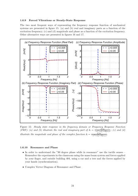
1.6.9 Forced Vibrations or Steady-State Response
The two most frequent ways of representing the frequency response function of mechanical
systems are presented in figure 15: (a) and (b) real and imaginary parts as a function of the
excitation frequency; (c) and (d) magnitude and phase as a function of the excitation frequency.
Other alternative ways are presented in figures 16 and 17.
(a) Frequency Response Function (Real Part)
5
ξ=0.005
ξ=0.05
Real(A(ω)) [m/N]
0
−5
0 0.5 1 1.5 2
Frequency [Hz]
(b) Frequency Response Function (Imaginary Part)
0
ξ=0.005
−2
ξ=0.05
Imag(A(ω)) [m/N]
−4
−6
−8
−10
0 0.5 1 1.5 2
Frequency [Hz]
Phase(A(ω)) [ o]
(c) Frequency Response Function (Amplitude)
10
ξ=0.005
8
ξ=0.05
||A(ω)|| [m/N]
6
4
2
−100
−150
0
0 0.5 1 1.5 2
Frequency [Hz]
(d) Frequency Response Function (Phase)
0
−50
ξ=0.005
ξ=0.05
−200
0 0.5 1 1.5 2
Frequency [Hz]
Figure 15: Steady state response in the frequency domain or Frequency Response Function
f/m
(FRF): (a) and (b) illustrate the real and imaginary part of A = −ω2 +ω2 n +i2ξωnω; (c) and (d)
illustrate the magnitude and phase of the complex function A =
1.6.10 Resonance and Phase
f/m
−ω 2 +ω 2 n+i2ξωnω .
• In order to understand the ”90 degree phase while in resonance” use the tactile senses –
Remember the experiments in the classroom using the mass-beam system and forces applied
by your finger, and outside building 404, using a car and a tree and the forces applied by
your hands (synchronization).
• Complex Vector Diagram of Resonance and Phase
24