Dynamics of Machines - Part II - IFS.pdf

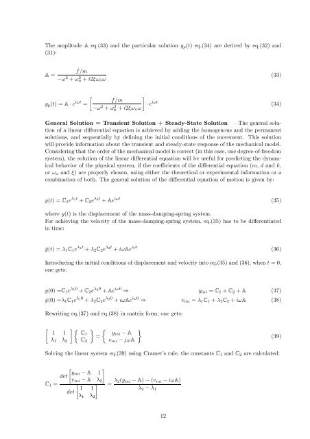
The amplitude A eq.(33) and the particular solution yp(t) eq.(34) are derived by eq.(32) and
(31):
A =
f/m
−ω 2 + ω 2 n + i2ξωnω
yp(t) = A · e iωt
=
f/m
−ω 2 + ω 2 n + i2ξωnω
· e iωt
General Solution = Transient Solution + Steady-State Solution – The general solution
of a linear differential equation is achieved by adding the homogenous and the permanent
solutions, and sequentially by defining the initial conditions of the movement. This solution
will provide information about the transient and steady-state response of the mechanical model.
Considering that the order of the mechanical model is correct (in this case, one degree-of-freedom
system), the solution of the linear differential equation will be useful for predicting the dynamical
behavior of the physical system, if the coefficients of the differential equation (m, d and k,
or ωn and ξ) are properly chosen, using either the theoretical or experimental information or a
combination of both. The general solution of the differential equation of motion is given by:
y(t) = C1e λ1t + C2e λ2t + Ae iωt
where y(t) is the displacement of the mass-damping-spring system.
For achieving the velocity of the mass-damping-spring system, eq.(35) has to be differentiated
in time:
˙y(t) = λ1C1e λ1t + λ2C2e λ2t + iωAe iωt
Introducing the initial conditions of displacement and velocity into eq.(35) and (36), when t = 0,
one gets:
y(0) =C1e λ10 + C2e λ20 + Ae iω0 ⇒ yini = C1 + C2 + A (37)
˙y(0) =λ1C1e λ10 + λ2C2e λ20 + iωAe iω0 ⇒ vini = λ1C1 + λ2C2 + iωA (38)
Rewriting eq.(37) and eq.(38) in matrix form, one gets:
1 1
λ1 λ2
C1
C2
=
yini − A
vini − jωA
Solving the linear system eq.(39) using Cramer’s rule, the constants C1 and C2 are calculated:
C1 =
yini − A 1
det
vini − A λ2
=
1 1
det
λ2(yini − A) − (vini − iωA)
λ2 − λ1
λ1 λ2
12
(33)
(34)
(35)
(36)
(39)