Relational Takagi–Sugeno Models for Rainfall ... - EUSFLAT

Relational Takagi–Sugeno Models for Rainfall-Discharge Modeling
Hilde Vernieuwe
Department of Applied Mathematics,
Biometrics and Process Control
Ghent University
Coupure links 653, 9000 Gent, Belgium
Hilde.Vernieuwe@rug.ac.be
Abstract
In this paper, the use of fuzzy models relating
rainfall to catchment discharge is investigated
for the Zwalm catchment in Belgium.
The models are built along the lines
of Gaweda’s method [4]. Since acceptable
models were not obtained for this data set,
the method was further adapted. The newly
obtained models are of comparable performance
as Takagi–Sugeno models based on
the Gustafson–Kessel clustering algorithm.
Keywords: Gustafson–Kessel clustering,
rainfall-discharge, relational rules, Takagi–
Sugeno models.
1 Introduction
With respect to rainfall-discharge prediction some
models using fuzzy rules have been reported over
the past years. See and Openshaw [8] used a combination
of a hybrid neural network, an autoregressive
moving average model, and a simple fuzzy rulebased
model for discharge forecasting. Hundecha
et al. [5] developed fuzzy rule-based routines simulating
different processes involved in the generation
of discharge from precipitation inputs, and incorporated
them in the modular conceptual physical
model of Bergstrom [2]. Finally, Xiong et al. [11]
used a Takagi–Sugeno model in a flood forecasting
study, combining the forecasts of five different
rainfall-discharge models.
In [10], we developed different Takagi–Sugeno models
using three different identification methods for
identifying the antecedent parts: grid partitioning,
Bernard De Baets
Department of Applied Mathematics,
Biometrics and Process Control
Ghent University
Coupure links 653, 9000 Gent, Belgium
Bernard.DeBaets@rug.ac.be
subtractive clustering and Gustafson–Kessel clustering.
The results in that paper show that Takagi–
Sugeno models with antecedent parts determined by
the Gustafson–Kessel clustering method and with linear
consequent parts (GKL) give the best results.
In this paper, we investigate whether comparable results
can be obtained using a Takagi–Sugeno model
with relational rules. The relational rules are identified
using the method presented in [4].
2 Study Area and Data Used
The Takagi–Sugeno models developed in this paper
have been applied to predict the discharge of the river
Zwalm in Belgium. Troch et al. [9] give a general
overview of the soil, vegetative, and topographic conditions
of the catchment.
The data set consists of hourly precipitation values
(obtained through disaggregation of daily observations)
and hourly measured discharge values from
1994 through 1998. Pauwels et al. [7] describe in detail
this precipitation disaggregation algorithm.
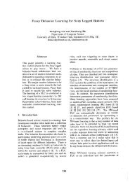
The identification data set used to build the models
consists of the data set for 1994 only (Fig. 1). The
entire data set was then used for validation. The discharge
records show a high temporal variability, and
include extremely high and low values. Since the
hourly precipitation records were obtained using daily
observations, the model performance was evaluated
using both hourly and daily averages of simulated and
observed discharge values.

Q(t+1)
20
15
10
5
0
20
15
10
Q(t)
5
0 0
Figure 1: Identification data
3 Relational Rules for the Zwalm
Catchment
The Takagi–Sugeno models used will predict the discharge
value Q at time step t + 1 using the precipitation
and discharge values P and Q at the previous time
step t. The Takagi–Sugeno model uses relational rules
of the form:
IF(P(t),Q(t)) is Ri THEN Q(t + 1) =
2
4
P(t)
aiP(t)+biQ(t)+ci
where Ri is a fuzzy relation on the Cartesian products
of the domains of P and Q [4]. In this particular
case, the fuzzy relation R is considered as a twodimensional
membership function. Q(t + 1) is computed
as:
Q(t + 1) = ∑n i=1 Ri(P(t),Q(t))(aiP(t)+biQ(t)+ci)
∑ n i=1 Ri(P(t),Q(t))
(1)
In order to identify the parameters of the rules, the
method presented in [4] is used. First, the Gustafson–
Kessel clustering method is applied on the data set
in the input-output space. From this clustering algorithm,
a fuzzy partition matrix is obtained. This
matrix contains the membership degrees of the data
points z = (x,y) to the different fuzzy clusters. From
this partition matrix, a subset Zi, corresponding to the
i-th cluster, is determined. This subset contains the
data points with a membership value to the i-th cluster
bigger than an arbitrarily chosen threshold α. For
each subset, the parameters of the two-dimensional
membership functions are determined: the center coordinates
for the i-th membership function:
c i = 1
Ni
Ni
∑ x
k=1
k
6
8
10
12
(2)
with Ni the number of data points in the subset Zi. The
standard deviation for the i-th membership function:
s i
∑
p =
Ni
k=1 (cip − xk p) 2
(3)
Ni − 1
with c i p and x k p the values of c i and x k for the p-th dimension.
The correlation coefficient for the i-th membership
function between the p-th and the q-th dimen-
sions:
r i pq =
∑ N i
k=1 (ci p−x k p)(c i q−x k q)
Ni−1
s i ps i q
(4)
with x k p, x k q, c ip and c iq the values of x k and c i for the pth
and the q-th dimension. The membership functions
Gaweda uses are then:
−1
1−ri pq 2
xp−ci p
si 2
xq−ci q
+
p
si 2 −2r
q
i (xp−c
pq
i p )(xq−ciq )
si psi
q
Ri(xp,xq)=e
(5)
The vector ai = (ai,bi,ci) containing the consequent
parameters of rule i is then computed using:
ai = (X T
i Xi) −1 X T
i Yi
(6)
with Xi the matrix containing Ni rows of type (x k 1)
and Yi the vector containing the corresponding output
parts of the vectors of the subset Zi.
4 Modeling Results and Improvements
In order to examine the performance of the Takagi–
Sugeno models, the following two indices are used:
(i) The criterion of Nash and Suttcliffe [6] (NS),
commonly used in hydrological studies and comparable
to the Variance Accounted For (VAF),
compares the sum of squares of model errors
with the sum of squares of errors when “no
model” is present:
NS = 1 −
N
∑
k=1
N
∑
k=1
(Qm(k) − Qobs(k)) 2
(Qobs(k) − Qobs) 2
(7)
where Qm is the simulated discharge, Qobs is the
observed discharge and Qobs denotes the mean of
the observed data. The optimal value of NS is 1,
meaning a perfect match of the model. A value
of zero indicates that the model predictions are as

Table 1: Coordinates of the centra, with the corresponding
performance indices
Centra Coordinates NS RMSE
Model P(t) Q(t) [-] [m 3 s −1 ]
I 1.11 2.69 -77.33 16.49
0.01 1.70
II 0.05 3.44 -0.72 2.45
0.12 1.00
good as that of a “no-knowledge” model continuously
simulating the mean of the observed signal
[3]. Negative values indicate that the model
is performing worse than this “no-knowledge”
model [3].
(ii) The Root Mean Square Error (RMSE) given by:
N
∑(Qobs(k)
− Qm(k))
k=1
RMSE =
2
(8)
N
Using the above described method, the parameters of
the rules were identified. Since the Gustafson–Kessel
fuzzy clustering algorithm is an iterative clustering algorithm
with a random initialisation of the partition
matrix, the method was repeated 30 times. For the
Gustafson–Kessel clustering, the tolerance value was
set to 10 −3 and the fuzziness exponent was set to 2.
Since the optimal number of clusters found in [10]
was 2, the relational models were built using 2 clusters.
For each repetition, a relational rule base was
built and a baseline run was performed on the training
data. Within these 30 repetitions, essentially two different
values for the performance indices were found.
The corresponding models also have the same parameters,
i.e. centra, spreads, correlation coefficients and
consequent parameters, within a certain accuracy. Apparently,
for this data set, the Gustafson–Kessel clustering
algorithm can only convergence to two different
models. The coordinates of the centra, together with
the corresponding values of the performance indices
are given in Table 1. The values of the performance
indices show that these models do not perform gooed.
These poor values may be caused by the fact that data
points that have a higher value in rainfall and/or discharge
are not well covered by the membership functions.
This can be seen by comparing Figs. 1and 2.
Figure 2: Membership functions for one of the relational
models
In order to improve the relational models for this data
set, the covariance matrices Σi, and the cluster centra
mi, resulting from the Gustafson–Kessel clustering
algorithm, are used to construct the two-dimensional
membership functions. The two-dimensional membership
functions can then be scaled by introducing a
multiplicative parameter βi into each of the different
covariance matrices. In order to use a Gaussian-like
expression, the exponent in Eq. 5 is multiplied by 0.5.
Eq. 5 can then be rewritten as:
Ri(xp,xq) = e −0.5(x−mi)(β 2 i Σi) −1 (x−mi) T
(9)
The consequent parameters were then estimated using
a global least squares method [1].
βi was varied between 1,2,3 and 4 for the two clusters
separately. For each combination of the two βi’s, the
covariance matrices and the cluster centra of the previous
30 models were used to build new models. A
baseline run was performed on the training data. The
values of the performance indices for the best models
found with the above described combinations of
β’s varied between 0.11 and 0.45 for NS and 1.75 and
1.38 for RMSE. The models with the best values for
both NS= 0.45 and RMSE= 1.38, were found with 2
and 4 as βi’s. These best models are built using model
type I of Tabel 1, with the covariance matrix of the
first cluster multiplied by 4 and the covariance matrix
of the second cluster multiplied by 16. Fig. 3 shows
the membership functions for one of these models.
These best models were then used to perform a baseline
run on the entire data set. The performance indices
are calculated using the mean output of these
models (Table 2). The values of the performance indices
for the GKL models are also listed (Table 2).
From this table, one can see that both methods yield

Figure 3: Membership functions for one of the relational
models
Table 2: Values of the performance indices for the
baseline run on the entire data set using the relational
models and the GKL models
Relational GKL
NS hourly 0.43 0.43
[-] daily 0.48 0.47
RMSE hourly 1.37 1.37
[m 3 s −1 ] daily 1.18 1.19
comparable results. The modeling results for the relational
models for 1998 are shown in Fig. 4.
5 Conclusion
Relational rules were used to develop data-driven
Takagi–Sugeno models. Applying the method as described
by [4] dit not result in acceptable models. This
can be due to the fact that the membership functions
are too narrow compared to the spread of the training
data. Multiplying the covariance matrices by a factor
β2 i , did result in broader membership functions and
model results that are comparable to those obtained
Q(m3/s)
16
14
12
10
8
6
4
2
0
0 50 100 150 200 250 300 350
Day of year
Figure 4: Simulation results for the relational models
for 1998. The observations are in solid lines and the
simulations are in dashed lines.
0
20
40
60
80
100
120
140
P(mm/day)
by the GKL models.
Acknowledgements
The authors would like to thank A. Gaweda for the
use of his software.
References
[1] R. Babuˇska, Fuzzy Modeling for Control,
Kluwer Academic Publishers, 1998.
[2] S. Bergström, The HBV model, Computer Models
of Watershed Hydrology (V. P. Singh, ed.),
Water Resources Publications, 1995, pp. 443–
476.
[3] K.J. Beven, Rainfall-Runoff Modelling, The
Primer, John Wiley and Sons, 2000.
[4] A.E. Gaweda, Optimal data-driven rule extraction
using adaptive fuzzy-neural models, Ph.D.
thesis, University of Louisville, Lousville, Kentucky,
August 2002.
[5] Y. Hundecha, A. Bárdossy, and H.W. Theisen,
Development of a fuzzy logic-based rainfallrunoff
model, Hydrol. Sc. Journal 46 (2001),
no. 3, 363–376.
[6] J.E. Nash and J.V. Sutcliffe, River flow forecasting
through conceptual models part I - a discussion
of principles, J. Hydrol. 10 (1970), 282–
290.
[7] V. R. N. Pauwels, N. E. C. Verhoest, and F. P.
De Troch, A meta-hillslope model based on an
analytical solution to the linearized Boussinesqequation
for temporally variable recharge rates,
Water Resour. Res. 38 (2002), no. 12, 1297,
doi:1029/2001WR000714.
[8] L. See and S. Openshaw, A hybrid multi-model
approach to river level forecasting, Hydrol. Sci.
Journal 45 (2000), no. 4, 523–536.
[9] P.A. Troch, F.P. De Troch, and W. Brutsaert, Effective
water table depth to describe initial conditions
prior to storm rainfall in humid regions,
Water Resour. Res. 29 (1993), no. 2, 427–434.
[10] H. Vernieuwe, O. Georgieva, B. De Baets,
V.R.N. Pauwels, and N.E.C. Verhoest, Fuzzy
models of rainfall-discharge dynamics, Lecture
Notes in Computer Science, to appear.
[11] L. Xiong, A.Y. Shamseldin, and K.M.
O’Connor, A non-linear combination of the
forecasts of rainfall-runoff models by the firstorder
Takagi-Sugeno fuzzy system, J. Hydrol.
245 (2001), 196–217.