Sub-additivity re-examined: the case for Value-at-Risk - Eurandom
Sub-additivity re-examined: the case for Value-at-Risk - Eurandom
Sub-additivity re-examined: the case for Value-at-Risk - Eurandom

Create successful ePaper yourself
Turn your PDF publications into a flip-book with our unique Google optimized e-Paper software.
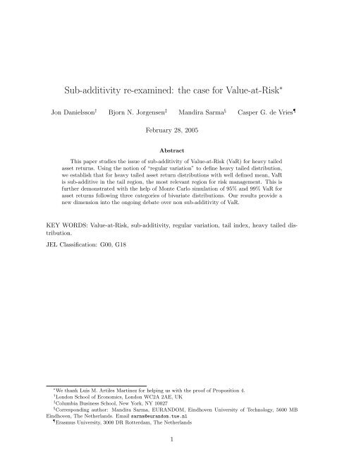
<strong>Sub</strong>-<strong>additivity</strong> <strong>re</strong>-<strong>examined</strong>: <strong>the</strong> <strong>case</strong> <strong>for</strong> <strong>Value</strong>-<strong>at</strong>-<strong>Risk</strong> ∗<br />
Jon Danielsson † Bjorn N. Jorgensen ‡ Mandira Sarma § Casper G. de Vries <br />
February 28, 2005<br />
Abstract<br />
This paper studies <strong>the</strong> issue of sub-<strong>additivity</strong> of <strong>Value</strong>-<strong>at</strong>-<strong>Risk</strong> (VaR) <strong>for</strong> heavy tailed<br />
asset <strong>re</strong>turns. Using <strong>the</strong> notion of “<strong>re</strong>gular vari<strong>at</strong>ion” to define heavy tailed distribution,<br />
we establish th<strong>at</strong> <strong>for</strong> heavy tailed asset <strong>re</strong>turn distributions with well defined mean, VaR<br />
is sub-additive in <strong>the</strong> tail <strong>re</strong>gion, <strong>the</strong> most <strong>re</strong>levant <strong>re</strong>gion <strong>for</strong> risk management. This is<br />
fur<strong>the</strong>r demonstr<strong>at</strong>ed with <strong>the</strong> help of Monte Carlo simul<strong>at</strong>ion of 95% and 99% VaR <strong>for</strong><br />
asset <strong>re</strong>turns following th<strong>re</strong>e c<strong>at</strong>egories of bivari<strong>at</strong>e distributions. Our <strong>re</strong>sults provide a<br />
new dimension into <strong>the</strong> ongoing deb<strong>at</strong>e over non sub-<strong>additivity</strong> of VaR.<br />
KEY WORDS: <strong>Value</strong>-<strong>at</strong>-<strong>Risk</strong>, sub-<strong>additivity</strong>, <strong>re</strong>gular vari<strong>at</strong>ion, tail index, heavy tailed distribution.<br />
JEL Classific<strong>at</strong>ion: G00, G18<br />
∗ We thank Luis M. Artiles Martinez <strong>for</strong> helping us with <strong>the</strong> proof of Proposition 4.<br />
† London School of Economics, London WC2A 2AE, UK<br />
‡ Columbia Business School, New York, NY 10027<br />
§ Cor<strong>re</strong>sponding author: Mandira Sarma, EURANDOM, Eindhoven University of Technology, 5600 MB<br />
Eindhoven, The Ne<strong>the</strong>rlands. Email sarma@eurandom.tue.nl<br />
Erasmus University, 3000 DR Rotterdam, The Ne<strong>the</strong>rlands<br />
1
1 Introduction<br />
<strong>Value</strong>-<strong>at</strong>-<strong>Risk</strong> (VaR) has been widely accepted as a tool <strong>for</strong> financial risk management. The<br />
Basel Committee’s <strong>re</strong>commend<strong>at</strong>ion <strong>for</strong> VaR in 1996 (Basel Committee on Banking Supervision,<br />
1996) and <strong>re</strong>cently proposed Basel II norms (Basel Committee on Banking Supervision,<br />
2003) have heightened <strong>the</strong> importance of VaR as a market risk measu<strong>re</strong>. Following <strong>the</strong> guidelines<br />
of <strong>the</strong> Basel Committee, financial <strong>re</strong>gul<strong>at</strong>ors all over <strong>the</strong> world have adopted VaR <strong>for</strong><br />
designing capital adequacy standard <strong>for</strong> banks and financial institutions. Apart from financial<br />
<strong>re</strong>gul<strong>at</strong>ors like central banks and Securities Exchange <strong>re</strong>gul<strong>at</strong>ors, financial firms have adopted<br />
VaR <strong>for</strong> internal risk management and alloc<strong>at</strong>ion of <strong>re</strong>sources.<br />
Despite its global <strong>re</strong>cognition as a measu<strong>re</strong> of financial risk, VaR has been criticised on certain<br />
<strong>the</strong>o<strong>re</strong>tical grounds. Artzner et al. (1997) and Artzner et al. (1999) have criticised VaR <strong>for</strong> not<br />
s<strong>at</strong>isfying <strong>the</strong> conditions of a “cohe<strong>re</strong>nt” risk measu<strong>re</strong>. The axioms of “cohe<strong>re</strong>ncy” comprise<br />
four ma<strong>the</strong>m<strong>at</strong>ical properties, viz., monotonicity, positive homogeneity, transl<strong>at</strong>ion invariance<br />
and sub-<strong>additivity</strong>. VaR, being a tail-quantile, is not sub-additive in general, and <strong>the</strong><strong>re</strong>fo<strong>re</strong>,<br />
is not cohe<strong>re</strong>nt. VaR is sub-additive under <strong>the</strong> <strong>re</strong>strictive assumption of normally distributed<br />
asset <strong>re</strong>turns, which is a ra<strong>re</strong> situ<strong>at</strong>ion. since most often asset <strong>re</strong>turns a<strong>re</strong> found to be heavy<br />
tailed ra<strong>the</strong>r than normally distributed.<br />
In this paper we study <strong>the</strong> issue of non sub-<strong>additivity</strong> of VaR in <strong>the</strong> tail <strong>re</strong>gion of heavy tailed<br />
asset <strong>re</strong>turns. Using <strong>the</strong> concept of “<strong>re</strong>gular vari<strong>at</strong>ion” to define heavy tails, we show th<strong>at</strong> <strong>for</strong><br />
heavy tailed distributions, VaR is sub-additive in <strong>the</strong> tail <strong>re</strong>gion. Thus, although VaR is not<br />
sub-additive <strong>for</strong> a generic distribution, <strong>at</strong> <strong>the</strong> tail <strong>re</strong>gion of heavy tailed distribution VaR does<br />
s<strong>at</strong>isfy sub-<strong>additivity</strong>. Keeping in view th<strong>at</strong> financial <strong>re</strong>turns a<strong>re</strong> often heavy tailed, coupled<br />
with <strong>the</strong> fact th<strong>at</strong> only <strong>the</strong> tail <strong>re</strong>gion is most <strong>re</strong>levant <strong>for</strong> risk management and not <strong>the</strong> enti<strong>re</strong><br />
distribution, this provides an inte<strong>re</strong>sting insight into <strong>the</strong> ongoing deb<strong>at</strong>e on <strong>the</strong> suitability of<br />
VaR as a risk measu<strong>re</strong>. This is specially <strong>re</strong>levant <strong>for</strong> st<strong>re</strong>ss testing th<strong>at</strong> <strong>re</strong>qui<strong>re</strong> estim<strong>at</strong>ion of<br />
ext<strong>re</strong>me quantiles, lying far out in <strong>the</strong> tail <strong>re</strong>gion.<br />
This paper is organised as follows: Section 2 discusses <strong>the</strong> concept of sub-<strong>additivity</strong>, along with<br />
a brief <strong>re</strong>view of <strong>the</strong> sub-<strong>additivity</strong> deb<strong>at</strong>e. Section 3 discusses <strong>the</strong> concept of “<strong>re</strong>gular vari<strong>at</strong>ion”<br />
and defines heavy-tailed distributions as those with “<strong>re</strong>gularly varying” tails. In Section<br />
4 we discuss sub-<strong>additivity</strong> of VaR <strong>at</strong> <strong>the</strong> tail <strong>re</strong>gion and establish th<strong>at</strong> VaR is sub-additive in<br />
<strong>the</strong> tail a<strong>re</strong>a <strong>for</strong> distributions with well-defined first moment. This is fur<strong>the</strong>r demonstr<strong>at</strong>ed in<br />
Section 5 with <strong>the</strong> help of Monte Carlo simul<strong>at</strong>ion to display <strong>the</strong> sub-<strong>additivity</strong> of 95% and<br />
99% VaR <strong>for</strong> simul<strong>at</strong>ed asset <strong>re</strong>turns belonging to th<strong>re</strong>e c<strong>at</strong>egories of bivari<strong>at</strong>e distributions.<br />
Section 6 concludes <strong>the</strong> paper.<br />
2 <strong>Sub</strong>-<strong>additivity</strong><br />
Let X and Y be two financial assets. A risk measu<strong>re</strong> ρ is sub-additive if <strong>the</strong> following is true.<br />
ρ(X + Y ) ≤ ρ(X) + ρ(Y ) (1)<br />
Thus, <strong>the</strong> risk measu<strong>re</strong> of <strong>the</strong> sum of two assets is bounded above by <strong>the</strong> sum of <strong>the</strong>ir individual<br />
2
isks. 1 The property of sub-<strong>additivity</strong> can be motiv<strong>at</strong>ed by many practical consider<strong>at</strong>ions.<br />
<strong>Sub</strong>-<strong>additivity</strong> ensu<strong>re</strong>s th<strong>at</strong> <strong>the</strong> diversific<strong>at</strong>ion principle of modern portfolio <strong>the</strong>ory holds. A<br />
sub-additive measu<strong>re</strong> would always gener<strong>at</strong>e a lower risk measu<strong>re</strong> <strong>for</strong> a diversified portfolio<br />
than a non-diversified portfolio. In terms of internal risk management, sub-<strong>additivity</strong> also<br />
implies th<strong>at</strong> <strong>the</strong> overall risk of a financial firm can be added up to be equal to or less than<br />
<strong>the</strong> sum of <strong>the</strong> risks of individual departments of <strong>the</strong> firm. This appears to give an appealing<br />
dimension into <strong>the</strong> idea of integr<strong>at</strong>ed risk management. Fur<strong>the</strong>r, in <strong>the</strong> absence of sub<strong>additivity</strong>,<br />
a financial firm with risk X + Y would calcul<strong>at</strong>e a smaller <strong>re</strong>gul<strong>at</strong>ory capital of<br />
ρ(X) + ρ(Y ), leading to unde<strong>re</strong>stim<strong>at</strong>ion of risk <strong>re</strong>serve.<br />
It can be proved easily by constructing suitable examples th<strong>at</strong> VaR viol<strong>at</strong>es sub-<strong>additivity</strong><br />
property (Artzner et al., 1999; Acerbi & Tasche, 2001; Acerbi et al., 2001). The lack of sub<strong>additivity</strong><br />
of VaR has been seve<strong>re</strong>ly criticised, and several altern<strong>at</strong>ive measu<strong>re</strong>s have been<br />
proposed to <strong>re</strong>place VaR such as tail conditional expect<strong>at</strong>ion (TCE) and worst conditional<br />
expect<strong>at</strong>ion (WCE) by Artzner et al. (1999) and expected shortfall (ES) by Acerbi et al.<br />
(2001).<br />
It is however, argued th<strong>at</strong> “imposing sub-<strong>additivity</strong> <strong>for</strong> all risks (including dependent risks)<br />
is not in line with wh<strong>at</strong> could be called best practice” (Dhaene et al., 2003). 2 The measu<strong>re</strong><br />
of global risk may not be a priori smaller than <strong>the</strong> sum total of local risks. The following<br />
example <strong>at</strong>tempts to illustr<strong>at</strong>e this point.<br />
Consider a hypo<strong>the</strong>tical economy whe<strong>re</strong> <strong>the</strong><strong>re</strong> a<strong>re</strong> only two banks, viz. B1 and B2. Suppose<br />
th<strong>at</strong> B1 has only one investment project P1 and B2 has only one investment project P2, P1<br />
and P2 being independent, each project having exactly <strong>the</strong> same pay off structu<strong>re</strong> as follows:<br />
Pay-off Probability<br />
High profit (H)<br />
Low profit (L)<br />
High loss (-H)<br />
Low loss (-L)<br />
Thus, <strong>the</strong> probability of failu<strong>re</strong> of a bank is 1<br />
2 .<br />
Under this scenario, it is easy to show th<strong>at</strong><br />
1<br />
4<br />
1<br />
4<br />
1<br />
4<br />
1<br />
4<br />
Pr{At least one bank fails} = 3<br />
4<br />
Pr{Systemic failu<strong>re</strong>} = 1<br />
4<br />
Now, assume th<strong>at</strong> <strong>the</strong> two banks merge. Then, <strong>the</strong> hypo<strong>the</strong>tical economy has just one bank,<br />
investing in two independent projects P1 and P2 with <strong>the</strong> pay-off structu<strong>re</strong> from each project<br />
1 “...a merger does not c<strong>re</strong><strong>at</strong>e extra risk” (Artzner et al., 1999). However it depends. Merger usually c<strong>re</strong><strong>at</strong>es<br />
positive diversific<strong>at</strong>ion effect but might inc<strong>re</strong>ase <strong>the</strong> systemic risk. See example th<strong>at</strong> follows.<br />
2 Dhaene et al. (2003) have also argued th<strong>at</strong> <strong>the</strong> axioms of “cohe<strong>re</strong>nce” leads to a very <strong>re</strong>strictive set of risk<br />
measu<strong>re</strong>s th<strong>at</strong> cannot be used in practical situ<strong>at</strong>ions.<br />
3
as given above. Under this scenario it is easily shown th<strong>at</strong><br />
Pr{Bank fails} = 6<br />
16<br />
Pr{Systemic failu<strong>re</strong>} = 6<br />
16<br />
Thus, <strong>the</strong> probability of bank failu<strong>re</strong> <br />
6<br />
16 is less in <strong>the</strong> second scenario than th<strong>at</strong> in <strong>the</strong> first<br />
scenario <br />
3<br />
4 . This implies th<strong>at</strong> <strong>the</strong> diversific<strong>at</strong>ion effect of <strong>the</strong> merger has <strong>re</strong>duced <strong>the</strong> risk of<br />
<strong>the</strong> bank failu<strong>re</strong>.<br />
As far as <strong>the</strong> global risk is concerned, in <strong>the</strong> first scenario, systemic b<strong>re</strong>akdown occurs when<br />
both <strong>the</strong> banks fail and in <strong>the</strong> second scenario this occurs when <strong>the</strong> merged bank fails. In<br />
this example we see th<strong>at</strong> <strong>the</strong> probability of systemic failu<strong>re</strong> is higher in <strong>the</strong> second scenario<br />
( 6<br />
1<br />
16 ) than th<strong>at</strong> in <strong>the</strong> first scenario ( 4 )! Thus, <strong>the</strong> merger has led to an inc<strong>re</strong>ase in <strong>the</strong> global<br />
risk, despite <strong>the</strong> benefit of diversific<strong>at</strong>ion. 3<br />
This simple example illustr<strong>at</strong>es th<strong>at</strong> <strong>the</strong> diversific<strong>at</strong>ion does not necessarily lead to a <strong>re</strong>duction<br />
in <strong>the</strong> global risk. From this point of view sub-<strong>additivity</strong> may not depict <strong>the</strong> complex n<strong>at</strong>u<strong>re</strong><br />
of <strong>the</strong> financial markets.<br />
As <strong>the</strong> deb<strong>at</strong>e over <strong>the</strong> <strong>re</strong>qui<strong>re</strong>ment of sub-<strong>additivity</strong> (or, <strong>for</strong> th<strong>at</strong> m<strong>at</strong>ter, <strong>the</strong> axioms of<br />
cohe<strong>re</strong>nce) continues, we take a f<strong>re</strong>sh look <strong>at</strong> VaR <strong>for</strong> heavy tailed asset <strong>re</strong>turn distribution.<br />
We p<strong>re</strong>sent a new dimension into <strong>the</strong> deb<strong>at</strong>e by establishing th<strong>at</strong> VaR is sub-additive in <strong>the</strong><br />
tail <strong>re</strong>gions of heavy tailed distributions.<br />
3 Heavy tailed asset <strong>re</strong>turns and Regular Vari<strong>at</strong>ion<br />
Empirical studies have established th<strong>at</strong> <strong>the</strong> distribution of specul<strong>at</strong>ive asset <strong>re</strong>turns tend to<br />
have heavier tails than <strong>the</strong> normal distribution tails (Mandelbrot, 1963; Pagan, 1996; Engle,<br />
1982; Jansen & de Vries, 1991). Heavy tailed distributions a<strong>re</strong> often defined in terms of higher<br />
than normal kurtosis. However, <strong>the</strong> kurtosis of a distribution may be high if ei<strong>the</strong>r <strong>the</strong> tails<br />
of <strong>the</strong> cdf a<strong>re</strong> heavier than <strong>the</strong> normal or if <strong>the</strong> center is mo<strong>re</strong> peaked, or both. Fur<strong>the</strong>r, it<br />
is not only <strong>the</strong> higher than normal kurtosis, but also failu<strong>re</strong> of higher moments th<strong>at</strong> define<br />
heavy tails.<br />
In this paper we define heavy tailed distribution as one characterised by <strong>the</strong> failu<strong>re</strong> of <strong>the</strong><br />
moments of order m (> 0) or higher. Such distributions have tails th<strong>at</strong> exhibit a power type<br />
behaviour like <strong>the</strong> Pa<strong>re</strong>to distribution, as commonly observed in finance. Such tail behaviour<br />
can be ma<strong>the</strong>m<strong>at</strong>ically defined by using <strong>the</strong> notion of “<strong>re</strong>gular vari<strong>at</strong>ion”, as defined below 4 .<br />
Definition: A cdf F (x) varies <strong>re</strong>gularly <strong>at</strong> minus infinity with tail index α > 0 if<br />
F (−tx)<br />
lim<br />
t→∞ F (−t) = x−α ∀x > 0 (2)<br />
3<br />
One can easily generalise this example to incorpor<strong>at</strong>e mo<strong>re</strong> complex financial entities, and still come up<br />
with similar argument.<br />
4<br />
For an encyclopedic t<strong>re</strong><strong>at</strong>ment of <strong>re</strong>gular vari<strong>at</strong>ion, see Bingham et al. (1987); Resnick (1987).<br />
4
This implies th<strong>at</strong>, to a first order approxim<strong>at</strong>ion, all distributions have a tail comparable to<br />
<strong>the</strong> Pa<strong>re</strong>to distribution:<br />
This implies, <strong>for</strong> large x,<br />
F (−x) = Ax −α [1 + o(1)], x > 0, <strong>for</strong> α > 0 and A > 0 (3)<br />
f(−x) ≈ αAx −α−1 x > 0, <strong>for</strong> α > 0 and A > 0 (4)<br />
so th<strong>at</strong> <strong>the</strong> density declines <strong>at</strong> a power r<strong>at</strong>e x −α−1 far to <strong>the</strong> left of <strong>the</strong> cent<strong>re</strong> of <strong>the</strong> distribution<br />
which contrasts with <strong>the</strong> exponentially fast declining tails of <strong>the</strong> Gaussian distribution. This<br />
power is outweighed by <strong>the</strong> explosion of x m in <strong>the</strong> comput<strong>at</strong>ion of moments of order m ≥ α.<br />
Thus, moments of order m ≥ α a<strong>re</strong> unbounded and <strong>the</strong><strong>re</strong>fo<strong>re</strong> <strong>the</strong>se distributions display<br />
heavy tailed behaviour. The power α is called <strong>the</strong> tail index and it determines <strong>the</strong> number<br />
of bounded moments. It is <strong>re</strong>adily verified th<strong>at</strong> Student–t distributions, among o<strong>the</strong>rs, vary<br />
<strong>re</strong>gularly <strong>at</strong> infinity, has deg<strong>re</strong>es of f<strong>re</strong>edom equal to <strong>the</strong> tail index and s<strong>at</strong>isfies <strong>the</strong> above<br />
approxim<strong>at</strong>ion. Likewise, <strong>the</strong> st<strong>at</strong>ionary distribution of <strong>the</strong> popular GARCH(1,1) process has<br />
<strong>re</strong>gularly varying tails, see de Haan et al. (1989).<br />
Fur<strong>the</strong>r, to a second order approxim<strong>at</strong>ion, <strong>the</strong> tail of a <strong>re</strong>gularly varying cdf can be approxim<strong>at</strong>ed<br />
as<br />
<br />
−α<br />
F (−x) = Ax 1 + Bx −β <br />
+ O x −β<br />
, as x → ∞ (5)<br />
4 <strong>Sub</strong>-<strong>additivity</strong> of VaR in <strong>the</strong> tail<br />
In this section, we examine sub-<strong>additivity</strong> of VaR <strong>at</strong> <strong>the</strong> tail <strong>re</strong>gion of heavy tailed distributions<br />
defined as above. We consider only <strong>the</strong> lower tail. 5<br />
In <strong>the</strong> following, we assume th<strong>at</strong> X and Y a<strong>re</strong> two asset <strong>re</strong>turns, each having a <strong>re</strong>gularly<br />
varying tail with tail index α > 0. In this paper we consider only <strong>the</strong> <strong>case</strong> whe<strong>re</strong> <strong>the</strong> two<br />
asset <strong>re</strong>turns have equal tail index and equal or unequal tail coefficients. If <strong>the</strong> tail coefficients<br />
a<strong>re</strong> equal <strong>the</strong>n <strong>the</strong> asset <strong>re</strong>turns have identical tails while <strong>the</strong> tails a<strong>re</strong> non-identical if <strong>the</strong><br />
tail coefficients a<strong>re</strong> diffe<strong>re</strong>nt. Thus, we assume th<strong>at</strong> <strong>the</strong> source of non-identical tail behaviour<br />
arises from <strong>the</strong> differing values of <strong>the</strong> tail coefficients. 6<br />
We consider <strong>the</strong> <strong>case</strong> of independent X and Y in Section 4.1 and <strong>the</strong> <strong>case</strong> whe<strong>re</strong> X and Y<br />
a<strong>re</strong> dependent in Section 4.2.<br />
5<br />
For defining <strong>the</strong> upper tails of a heavy tailed distributions, we may use <strong>the</strong> notion of “<strong>re</strong>gular vari<strong>at</strong>ion”<br />
<strong>at</strong> plus infinity and carry on with an analogous proof.<br />
6<br />
Some empirical studies have found th<strong>at</strong> most asset <strong>re</strong>turns distributions tend to display equal tail coefficients<br />
but do differ considerably with <strong>re</strong>spect to <strong>the</strong>ir scale coefficients. See, eg. Hyung & de Vries (2002).<br />
5
4.1 Case of independent assets<br />
Proposition 1 Suppose th<strong>at</strong> X and Y a<strong>re</strong> two independent asset <strong>re</strong>turns both having <strong>re</strong>gularly<br />
varying tails with index α > 0 and scale coefficients A > 0 and B > 0. Then <strong>for</strong> α > 1 VaR<br />
is sub-additive in <strong>the</strong> tail <strong>re</strong>gion, <strong>re</strong>gardless of whe<strong>the</strong>r or not A = B.<br />
Proof:<br />
See Appendix A.1.<br />
Thus, if we assume th<strong>at</strong> α > 1, so th<strong>at</strong> <strong>the</strong> mean of <strong>the</strong> assets a<strong>re</strong> well defined, <strong>the</strong>n sub<strong>additivity</strong><br />
of VaR is established. The <strong>case</strong> of α ≤ 1, or <strong>the</strong> <strong>case</strong> of unbounded mean is very<br />
ra<strong>re</strong> in finance, and <strong>the</strong><strong>re</strong>fo<strong>re</strong> <strong>the</strong> assumption of α > 1 is not un<strong>re</strong>asonable <strong>for</strong> financial assets.<br />
4.1.1 Second order approxim<strong>at</strong>ion<br />
The second order tail approxim<strong>at</strong>ion (5) approxim<strong>at</strong>es a much larger a<strong>re</strong>a in <strong>the</strong> tail than <strong>the</strong><br />
first order approxim<strong>at</strong>ion.<br />
We can show th<strong>at</strong> even a second order approxim<strong>at</strong>ion of <strong>the</strong> tails, when such an approxim<strong>at</strong>ion<br />
is valid, can display VaR sub-<strong>additivity</strong> in some <strong>case</strong>s.<br />
For example, suppose th<strong>at</strong> X and Y a<strong>re</strong> two independent asset <strong>re</strong>turns, each having <strong>re</strong>gularly<br />
varying tails with <strong>the</strong> second order approxim<strong>at</strong>ion as in (5) with identical tail indexes and<br />
identical tail coefficients.<br />
Applic<strong>at</strong>ion of <strong>the</strong> Bruijn’s <strong>the</strong>ory of asymptotic inversion (Bingham et al., 1987) (pages<br />
28-29) leads to <strong>the</strong> following <strong>re</strong>sults<br />
V aRp(X) ≈ A 1<br />
<br />
1<br />
− α p α<br />
V aRp(Y ) ≈ A 1 1<br />
− α p α<br />
V aRp(X) + V aRp(Y ) ≈ 2A 1 1<br />
− α p α<br />
1 + B<br />
α<br />
<br />
1 + B<br />
α<br />
<br />
β<br />
A− α p β<br />
<br />
α<br />
β<br />
A− α p β<br />
<br />
α<br />
1 + B β<br />
A− α p<br />
α β<br />
α<br />
Proposition 2 If X and Y a<strong>re</strong> independent <strong>re</strong>turns with <strong>re</strong>gularly varying tails, each following<br />
<strong>the</strong> second order approxim<strong>at</strong>ion (5) with identical tail index and identical scale coefficients,<br />
<strong>the</strong>n V aRp(X + Y ) can be approxim<strong>at</strong>ed by <strong>the</strong> following exp<strong>re</strong>ssion.<br />
V aRp(X + Y ) ≈ (2A) 1<br />
<br />
1<br />
− α p α 1 + B<br />
<br />
p<br />
β<br />
α<br />
+<br />
α 2A<br />
α + 1<br />
2 E(X2 <br />
p<br />
)<br />
2A<br />
Proof:<br />
See Appendix A.2.<br />
<br />
(6)<br />
(7)<br />
(8)<br />
2 <br />
α<br />
+ E(X) (9)<br />
Proposition 3 If X and Y a<strong>re</strong> independent <strong>re</strong>turns with <strong>re</strong>gularly varying tails, each following<br />
<strong>the</strong> second order approxim<strong>at</strong>ion (5) with identical tail index and identical scale coefficients,<br />
and if E(X) = 0, β < 2 and B > 0, <strong>the</strong>n VaR is sub-additive in <strong>the</strong> tail <strong>re</strong>gion.<br />
6
Proof:<br />
Using <strong>re</strong>sults from (6) to (9), and using <strong>the</strong> conditions E(X) = 0, β < 2 and B > 0, it is<br />
easy to show th<strong>at</strong><br />
V aRp(X + Y ) − V aRp(X) − V aRp(Y ) ≈ A 1 1<br />
− α p α<br />
< 0<br />
2 1 <br />
α − 2<br />
+ B<br />
α<br />
β<br />
A− α p β <br />
α<br />
2 1<br />
α<br />
β<br />
− α − 2<br />
<br />
Thus under <strong>the</strong>se specific assumptions, even a second order tail approxim<strong>at</strong>ion leads to VaR<br />
sub-<strong>additivity</strong>.<br />
4.2 Case of dependent assets<br />
It is well known th<strong>at</strong> financial assets a<strong>re</strong> not necessarily independent. In this section we<br />
consider <strong>the</strong> <strong>case</strong> whe<strong>re</strong> <strong>the</strong> assets a<strong>re</strong> assumed to be dependent.<br />
Suppose th<strong>at</strong> X1 and X2 a<strong>re</strong> two assets, not necessarily independent. The simplest way to<br />
model <strong>the</strong> dependence between X1 and X2 would be to introduce <strong>the</strong> dependence through a<br />
common market factor, as in <strong>the</strong> <strong>case</strong> of a single index market model, given below<br />
Xi = βi R + Qi, i = 1, 2 (10)<br />
whe<strong>re</strong> R denotes <strong>the</strong> <strong>re</strong>turn of <strong>the</strong> market portfolio, βi <strong>the</strong> market risk and Qi <strong>the</strong> idiosyncr<strong>at</strong>ic<br />
risk of asset Xi. In this model, <strong>the</strong> Qis and R a<strong>re</strong> independent of each o<strong>the</strong>r; fur<strong>the</strong>r Qis a<strong>re</strong><br />
<strong>the</strong>mselves independent of each o<strong>the</strong>r. Thus, <strong>the</strong> only source of cross-sectional dependence<br />
between X1 and X2 is <strong>the</strong> common market risk. The security specific risks Qi a<strong>re</strong> independent<br />
of each o<strong>the</strong>r and <strong>the</strong><strong>re</strong>fo<strong>re</strong> can be diversified away.<br />
Since R and Qi a<strong>re</strong> independent, we can use Feller’s convolution <strong>the</strong>o<strong>re</strong>m to approxim<strong>at</strong>e <strong>the</strong><br />
tails of X1 and X2, depending upon <strong>the</strong> tail behaviour of R, Q1 and Q2. We can fur<strong>the</strong>r use<br />
it to approxim<strong>at</strong>e <strong>the</strong> tail of X1 + X2. Thus, under such a model, we can proceed in a similar<br />
manner as in <strong>the</strong> <strong>case</strong> of independent asset <strong>re</strong>turns. To illustr<strong>at</strong>e this, we p<strong>re</strong>sent below one<br />
particular <strong>case</strong>, viz., <strong>the</strong> <strong>case</strong> whe<strong>re</strong> R, Q1 and Q2 have <strong>re</strong>gularly varying tails with <strong>the</strong> same<br />
tail index α, but with diffe<strong>re</strong>nt tail coefficients.<br />
Proposition 4 Suppose th<strong>at</strong> asset <strong>re</strong>turns X1 and X2 can be modelled by <strong>the</strong> single index<br />
market model, whe<strong>re</strong> R, Q1 and Q2 all have <strong>re</strong>gularly varying tails with tail index α > 0 and<br />
tail coefficients Ar > 0, A1 > 0 and A2 > 0 <strong>re</strong>spectively. If α > 1, <strong>the</strong>n under <strong>the</strong> assumption<br />
th<strong>at</strong> <strong>the</strong> distribution of R is symmetric, VaR is sub-additive in <strong>the</strong> tail <strong>re</strong>gion.<br />
Proof:<br />
See Appendix A.3<br />
In general, <strong>the</strong> single index market model (10) may not describe <strong>the</strong> true n<strong>at</strong>u<strong>re</strong> of <strong>the</strong><br />
dependence between X1 and X2 since Qi’s may not be cross sectionally independent, although<br />
each one of <strong>the</strong>m may be independent from <strong>the</strong> common market factor R. For example, apart<br />
from <strong>the</strong> market risk, <strong>the</strong> assets X1 and X2 may be dependent on an industry specific risk,<br />
depicted by <strong>the</strong> movement of an industry specific index S, also known as “sectoral index”<br />
7
in finance. Such industry specific factor may lead to dependence between Q1 and Q2. We<br />
may model such cross sectional dependence by generalising <strong>the</strong> model (10) by incorpor<strong>at</strong>ing<br />
a sector specific factor S.<br />
Xi = βi R + τi S + Qi, i = 1, 2 (11)<br />
whe<strong>re</strong> R is <strong>the</strong> market factor, S is <strong>the</strong> industry specific factor and Qi is <strong>the</strong> idiosyncr<strong>at</strong>ic<br />
risk of <strong>the</strong> asset Xi. In this model Qi is independent of R and S. Fur<strong>the</strong>r, Qi a<strong>re</strong> cross<br />
sectionally independent. In this model, τi is <strong>the</strong> industry specific risk of <strong>the</strong> asset Xi. If S has<br />
a <strong>re</strong>gularly varying tail with scale coefficient As and tail index α, <strong>the</strong>n under <strong>the</strong> assumption<br />
of symmetric tails <strong>for</strong> R and S, it can be shown in <strong>the</strong> similar manner as in Appendix A.3,<br />
th<strong>at</strong><br />
V aRp(X1) ≈ p 1<br />
α (|β1| α Ar + |τ1| α As + A1) 1<br />
α<br />
V aRp(X2) ≈ p 1<br />
α (|β2| α Ar + |τ2| α As + A2) 1<br />
α<br />
V aRp(X1 + X2) ≈ p 1<br />
α (|β1 + β2| α Ar + |τ1 + τ2| α As + A1 + A2) 1<br />
α<br />
Proceeding similarly as in <strong>the</strong> <strong>case</strong> of <strong>case</strong> of <strong>the</strong> single index market model above (Proposition<br />
4), one <strong>case</strong> easily establish th<strong>at</strong><br />
V aRp(X1 + X2) ≤ V aRp(X1) + V aRp(X2)<br />
One can generalise <strong>the</strong> model by introducing mo<strong>re</strong> factors in <strong>the</strong> dependence structu<strong>re</strong> between<br />
X1 and X2 and establish sub-<strong>additivity</strong> in an analogous manner.<br />
5 Simul<strong>at</strong>ion <strong>re</strong>sults<br />
In order to demonstr<strong>at</strong>e empirically <strong>the</strong> above <strong>re</strong>sults, we have carried out a set of simul<strong>at</strong>ions.<br />
In this section we p<strong>re</strong>sent <strong>the</strong> <strong>re</strong>sults from <strong>the</strong> simul<strong>at</strong>ions from th<strong>re</strong>e c<strong>at</strong>egories of bivari<strong>at</strong>e<br />
distributions: Student’s t, jump process and bivari<strong>at</strong>e garch. We simul<strong>at</strong>e from two sample<br />
sizes N = 10 3 and 10 6 , <strong>the</strong> <strong>for</strong>mer is chosen to mimic <strong>the</strong> <strong>re</strong>al world sample sizes, and <strong>the</strong> l<strong>at</strong>ter<br />
<strong>the</strong> asymptotics. The number of simul<strong>at</strong>ions from each sample size is S = 10000 and 200. In<br />
<strong>the</strong> simul<strong>at</strong>ions, p denotes <strong>the</strong> significance level of VaR and n denotes <strong>the</strong> number of <strong>case</strong>s<br />
whe<strong>re</strong><br />
V aRp(X1 + X2) > V aRp(X1) + V aRp(X2)<br />
5.1 Student’s t-distribution<br />
The Student’s t-distribution is widely applied in modeling financial <strong>re</strong>turns. It has a <strong>re</strong>gularly<br />
varying tail with tail index equal to its deg<strong>re</strong>es of f<strong>re</strong>edom and tail coefficient as below:<br />
A =<br />
Γ( ν+1<br />
2 )<br />
Γ( ν<br />
2 )<br />
8<br />
ν ν−1<br />
2<br />
√<br />
νπ
whe<strong>re</strong> ν is <strong>the</strong> deg<strong>re</strong>es of f<strong>re</strong>edom. Fur<strong>the</strong>r, <strong>for</strong> ν > 2 <strong>the</strong> tail of Student’s t-distribution<br />
s<strong>at</strong>isfy <strong>the</strong> second order approxim<strong>at</strong>ion (5) with β = 2, and B = − ν2<br />
2<br />
ν+1<br />
ν+2 .<br />
Suppose th<strong>at</strong> X1 is N draws from t (ν1) and X2 is N draws from t (ν1), both being iid. We <strong>the</strong>n<br />
provide a dependence structu<strong>re</strong> as follows. Suppose ρ is a cor<strong>re</strong>l<strong>at</strong>ion coefficients. Consider<br />
<strong>the</strong> Choleski decomposition of <strong>the</strong> covariance m<strong>at</strong>rix<br />
Then <strong>the</strong> d<strong>at</strong>a m<strong>at</strong>rix is given by<br />
⎛<br />
1<br />
⎞<br />
ρ<br />
Σ = ⎝ ⎠ = A<br />
ρ 1<br />
′ A<br />
X =<br />
X1<br />
X2<br />
Thus, <strong>the</strong> cor<strong>re</strong>l<strong>at</strong>ion between <strong>the</strong> two columns of X is ρ <strong>at</strong> least when <strong>the</strong> second moment is<br />
defined. The <strong>re</strong>sults from simul<strong>at</strong>ing <strong>the</strong>se d<strong>at</strong>a a<strong>re</strong> p<strong>re</strong>sented in Tables 1 and 2.<br />
As shown in <strong>the</strong>se tables, n, <strong>the</strong> number of times when sub-<strong>additivity</strong> fails is very high when<br />
ν1 = 1 and/or ν2 = 1. These a<strong>re</strong> <strong>the</strong> <strong>case</strong>s when <strong>the</strong> first moments of X1 and X2 a<strong>re</strong> not<br />
well defined. Existence of well-defined mean is a necessary assumption in our analysis <strong>for</strong><br />
sub-<strong>additivity</strong> to hold.<br />
When <strong>the</strong> deg<strong>re</strong>es of f<strong>re</strong>edom of <strong>the</strong> Student’s t-vari<strong>at</strong>es is higher than 1, <strong>the</strong>n <strong>the</strong> first moment<br />
is well defined. As shown in Tables 1 and 2 <strong>for</strong> well defined first moment, <strong>the</strong> viol<strong>at</strong>ion of<br />
sub-<strong>additivity</strong> is negligible or zero.<br />
5.2 Jump process<br />
x1 and x2 a<strong>re</strong> N draws from N (0, 1), whe<strong>re</strong> each process is subject to <strong>the</strong> occasional jump:<br />
in our <strong>case</strong><br />
<br />
xi,j =<br />
<br />
xi,j =<br />
<br />
A ′<br />
xi,j with probability a<br />
b + c, c˜U (0, d) with probability 1 − a<br />
xi,j with probability 0.995<br />
10 + c, c˜U (0, 0.2) with probability 0.005<br />
we <strong>the</strong>n introduce wh<strong>at</strong> we call joint event prob, denoted by q, which is <strong>the</strong> probability th<strong>at</strong><br />
on days when <strong>the</strong> x1 jumps, x2 also Jumps.<br />
Table 3 p<strong>re</strong>sents <strong>the</strong> <strong>re</strong>sults of <strong>the</strong> simul<strong>at</strong>ion from <strong>the</strong> jump process.<br />
5.3 BEKK GARCH<br />
we estim<strong>at</strong>e <strong>the</strong> parameters of a bivari<strong>at</strong>e GARCH model, specifically <strong>the</strong> BEKK <strong>for</strong>m with<br />
daily d<strong>at</strong>a from Microsoft and Goldman Sachs over four years. We <strong>the</strong>n simul<strong>at</strong>e from this<br />
9
model. Using <strong>the</strong>se simul<strong>at</strong>ed <strong>re</strong>sults, we estim<strong>at</strong>e VaRs of <strong>the</strong> individual <strong>re</strong>turns and <strong>the</strong>ir<br />
sum. In Table 4 we p<strong>re</strong>sent <strong>the</strong> <strong>re</strong>sults from <strong>the</strong> simul<strong>at</strong>ion. It is seen from this table th<strong>at</strong><br />
<strong>the</strong> number of sub-<strong>additivity</strong> failu<strong>re</strong> is close to zero.<br />
6 Conclusion<br />
In this paper we take a f<strong>re</strong>sh look <strong>at</strong> <strong>the</strong> issue of sub-<strong>additivity</strong> of VaR. We argue th<strong>at</strong> <strong>for</strong><br />
heavy tailed asset <strong>re</strong>turn distributions VaR is sub-additive in <strong>the</strong> tail <strong>re</strong>gion. We define heavy<br />
tailed distribution as one characterised by <strong>the</strong> failu<strong>re</strong> of moments of order m > 0 or higher.<br />
Using <strong>the</strong> notion of “<strong>re</strong>gular vari<strong>at</strong>ion” to describe such a tail behaviour, we establish th<strong>at</strong><br />
<strong>for</strong> distributions with well defined mean (m > 1), VaR is sub-additive <strong>at</strong> <strong>the</strong> tail <strong>re</strong>gion of<br />
<strong>the</strong> distribution. Thus in <strong>the</strong> <strong>re</strong>levant <strong>re</strong>gion <strong>for</strong> risk management, i.e., <strong>the</strong> tail <strong>re</strong>gion, VaR<br />
is sub-additive. We fur<strong>the</strong>r demonstr<strong>at</strong>e our <strong>re</strong>sults with <strong>the</strong> help of a set of Monte Carlo<br />
simul<strong>at</strong>ion of 99% and 95% VaR <strong>for</strong> asset <strong>re</strong>turns simul<strong>at</strong>ed from th<strong>re</strong>e c<strong>at</strong>egories of bivari<strong>at</strong>e<br />
distributions: Student’s t-distribution, jump processes and bivari<strong>at</strong>e garch processes.<br />
Our <strong>re</strong>sults provide a new insight into <strong>the</strong> sub-<strong>additivity</strong> deb<strong>at</strong>e and offers VaR to be still<br />
applicable <strong>for</strong> risk management despite its lack of sub-<strong>additivity</strong> in general.<br />
10
Refe<strong>re</strong>nces<br />
Acerbi, C. & Tasche, D. (2001), Expected Shortfall: a n<strong>at</strong>ural cohe<strong>re</strong>nt altern<strong>at</strong>ive to <strong>Value</strong><br />
<strong>at</strong> <strong>Risk</strong>, Abaxbank Working Paper arXiv:cond-m<strong>at</strong>/0105191.<br />
Acerbi, C., Nordio, C. & Sirtori, C. (2001), Expected Shortfall as a Tool <strong>for</strong> Financial <strong>Risk</strong><br />
Management, Abaxbank Working Paper arXiv:cond-m<strong>at</strong>/0102304.<br />
Artzner, P., Delbaen, F., Eber, J. M. & He<strong>at</strong>h, D. (1997), ‘Thinking cohe<strong>re</strong>ntly’, <strong>Risk</strong><br />
10(11), 68–71.<br />
Artzner, P., Delbaen, F., Eber, J. M. & He<strong>at</strong>h, D. (1999), ‘Cohe<strong>re</strong>nt Measu<strong>re</strong>s of Riak’,<br />
Ma<strong>the</strong>m<strong>at</strong>ical Finance 9, 203–228.<br />
Basel Committee on Banking Supervision (1996), Ammendment to <strong>the</strong> capital accord to<br />
incorpor<strong>at</strong>e market risks, Committee Report 24, Basel Committee on Banking Supervision,<br />
Basel, Switzerland.<br />
Basel Committee on Banking Supervision (2003), Consult<strong>at</strong>ive Document The New Basel<br />
Capital Accord, Committee <strong>re</strong>port, Basel Committee on Banking Supervision, Basel,<br />
Switzerland.<br />
Bingham, N. H., Goldie, C. M. & Teugels, J. L. (1987), Regular Vari<strong>at</strong>ion, Cambridge University<br />
P<strong>re</strong>ss, Cambridge.<br />
de Haan, L., Resnick, S. I., Rootzen, H. & de Vries, C. G. (1989), ‘Ext<strong>re</strong>mal Behaviour of Solutions<br />
to a Stochastic Diffe<strong>re</strong>nce Equ<strong>at</strong>ion with Applic<strong>at</strong>ions to Arch-Processes’, Stochastic<br />
Processes and <strong>the</strong>ir Applic<strong>at</strong>ions pp. 213–224.<br />
Dhaene, J., Goovaerts, M. J. & Kaas, R. (2003), ‘Economic Capital Alloc<strong>at</strong>ion Derived from<br />
<strong>Risk</strong> Masu<strong>re</strong>s’, North American Actuarial Journal 7(2), 44–56.<br />
Engle, R. (1982), ‘Auto<strong>re</strong>g<strong>re</strong>ssive Conditional Heteroscedasticity with Estim<strong>at</strong>es of <strong>the</strong> Variance<br />
of United Kingdom Infl<strong>at</strong>ion’, Econometrica 50, 987–1007.<br />
Feller, W. (1971), An Introduction to Probability Theory and Its Applic<strong>at</strong>ions, Vol. II, John<br />
Wiley & Sons.<br />
Garcia, R., Renault, E. & Tsafack, G. (2003), Proper Conditioning <strong>for</strong> Cohe<strong>re</strong>nt VaR in<br />
Portfolio Management, Unversite de Mont<strong>re</strong>al, CIRANO and CIREQ Working Paper.<br />
Hyung, N. & de Vries, C. G. (2002), ‘Portfolio Diversific<strong>at</strong>ion Effects and Regular Vari<strong>at</strong>ion<br />
in Financial D<strong>at</strong>a’, Journal of German St<strong>at</strong>istical Society 86, 69–82.<br />
Jansen, D. W. & de Vries, C. G. (1991), ‘On <strong>the</strong> F<strong>re</strong>quency of Large Stock Returns: Putting<br />
Booms and Busts into Perspective’, The Review of Economics and St<strong>at</strong>istics 73(1), 18–24.<br />
Loeve, M. (1963), Probability Theory, 3rd edn, Springer, New York.<br />
Mandelbrot, B. B. (1963), ‘The vari<strong>at</strong>ion of certain specul<strong>at</strong>ive prices’, Journal of Business<br />
36, 392 – 417.<br />
11
Pagan, A. (1996), ‘The econometrics of financial markets’, Journal of Empirical Finance 3, 15<br />
– 102.<br />
Resnick, S. I. (1987), Ext<strong>re</strong>me <strong>Value</strong>s, Regular Vari<strong>at</strong>ion and Point Process, Springer-Verlag.<br />
12
Appendix A<br />
A.1 Proof of Proposition 1<br />
Suppose th<strong>at</strong> X and Y a<strong>re</strong> two independent asset <strong>re</strong>turns both having <strong>re</strong>gularly varying tails<br />
such th<strong>at</strong><br />
Pr{X ≤ −x} ≈ A x −α<br />
Pr{Y ≤ −x} ≈ B x −α<br />
Then <strong>the</strong> V aR <strong>at</strong> p-level <strong>for</strong> X, denoted by V aRp(X), is given by<br />
Similarly,<br />
We consider <strong>the</strong> following <strong>case</strong>s:<br />
I. A = B 7 In this <strong>case</strong>,<br />
Pr{X ≤ V aRp(X)} ≈ p<br />
A [V aRp(X)] −α ≈ p<br />
V aRp(X) ≈<br />
V aRp(Y ) ≈<br />
1<br />
B α<br />
p<br />
A<br />
p<br />
V aRp(X) + V aRp(Y ) ≈ 2<br />
1<br />
α<br />
1<br />
A α<br />
p<br />
Using Feller’s convolution <strong>the</strong>o<strong>re</strong>m (Feller, 1971)(page 278), we have<br />
Thus it follows<br />
Pr{X + Y ≤ V aRp(X + Y )} ≈ p<br />
2 A [V aRp(X + Y )] −α ≈ p<br />
V aRp(X + Y ) ≈ 2 1<br />
α<br />
V aRp(X + Y ) − [V aRp(X) + V aRp(Y )] ≈<br />
Following <strong>case</strong>s may be conside<strong>re</strong>d<br />
1<br />
A α<br />
p<br />
1<br />
A α<br />
[2<br />
p<br />
1<br />
α − 2]<br />
7 Garcia et al. (2003) have <strong>examined</strong> this by using a diffe<strong>re</strong>nt approach than ours.<br />
13
(a) α = 1 : in this <strong>case</strong> V aRp(X + Y ) = V aRp(X) + V aRp(Y ) and <strong>the</strong><strong>re</strong>fo<strong>re</strong> VaR is<br />
additive.<br />
(b) 0 < α < 1 : in this <strong>case</strong> V aRp(X + Y ) > V aRp(X) + V aRp(Y ) and hence VaR is<br />
super-additive.<br />
(c) α > 1 : in this <strong>case</strong> V aRp(X + Y ) < V aRp(X) + V aRp(Y ) and hence VaR is<br />
sub-additive.<br />
II. A = B<br />
In this <strong>case</strong>, Feller’s <strong>the</strong>o<strong>re</strong>m gives<br />
Thus we get <strong>the</strong> VaR as:<br />
This gives<br />
Pr{X + Y ≤ −x} ≈ (A + B) x −α<br />
V aRp(X + Y ) ≈<br />
V aRp(X + Y ) − V aRp(X) − V aRp(Y ) ≈<br />
Following <strong>case</strong>s may be conside<strong>re</strong>d:<br />
A + B<br />
p<br />
1<br />
α<br />
1<br />
1 α <br />
(A + B)<br />
p<br />
1<br />
α − A 1<br />
α − B 1 <br />
α<br />
(a) α > 1: In this <strong>case</strong>, 1<br />
α < 1. Using Cα inequality (Loeve, 1963), (p. 155), it di<strong>re</strong>ctly<br />
follows th<strong>at</strong><br />
VaR is sub-additive in this <strong>case</strong><br />
(A + B) 1<br />
α ≤ A 1<br />
α + B 1<br />
α<br />
(b) α < 1: In this <strong>case</strong>, 1<br />
α > 1. Hence <strong>the</strong> Cα inequality gives<br />
(A + B) 1<br />
α ≤ 2 1<br />
α −1 (A 1<br />
α + B 1<br />
α )<br />
Thus VaR is not necessarily sub-additive in this <strong>case</strong>.<br />
A.2 Proof of Proposition 2<br />
Suppose th<strong>at</strong> X and Y a<strong>re</strong> two independent asset <strong>re</strong>turns, each having <strong>re</strong>gularly varying tails<br />
with <strong>the</strong> following identical second order approxim<strong>at</strong>ion<br />
Pr{X ≤ −x} =<br />
<br />
−α<br />
Pr{X > x} = Ax 1 + Bx −β + o(x −α <br />
)<br />
Pr{Y ≤ −x} =<br />
<br />
−α<br />
Pr{Y > x} = Ax 1 + Bx −β + o(x −α <br />
)<br />
whe<strong>re</strong> α > 2, β > 0, A > 0 and B ∈ R 1 − {0}<br />
14
Following <strong>the</strong> second order convolution <strong>re</strong>sult from Dacorogna et al (1998) and de Vries (1999),<br />
we have,<br />
Pr{X + Y > x} = Pr{X + Y ≤ −x} ≈ 2Ax −α<br />
<br />
1 + Bx −β + αE(X)x −1 + 1<br />
2 α(α + 1)E(X2 )x −2<br />
<br />
whe<strong>re</strong> E(X) = E(Y ) and E(X 2 ) = E(Y 2 )<br />
Let p = Pr{X + Y ≤ −x}. Then,<br />
p ≈ 2Ax −α<br />
<br />
1 + Bx −β + αE(X)x −1 + 1<br />
2 α(α + 1)E(X2 )x −2<br />
p<br />
2A<br />
≈<br />
<br />
<br />
x−α 1 + Bx −β + αE(X)x −1 + 1<br />
2 α(α + 1)E(X2 )x −2<br />
y ≈<br />
<br />
x −α<br />
<br />
1 + Bx −β + αE(X)x −1 + 1<br />
2 α(α + 1)E(X2 )x −2<br />
<br />
whe<strong>re</strong> y = p<br />
2A (12)<br />
x ≈<br />
<br />
1<br />
−<br />
y α 1 + Bx −β + αE(X)x −1 + 1<br />
2 α(α + 1)E(X2 )x −2<br />
1<br />
α<br />
Clearly,<br />
1<br />
−<br />
= y α g (x(y))<br />
1 1<br />
− −<br />
= y α + y α {g (x(y)) − 1}<br />
1<br />
−<br />
= y α + ɛ(y) say (13)<br />
ɛ(y)<br />
1<br />
− y α<br />
Using (13) in (12), we have <strong>the</strong> following:<br />
y ≈<br />
Thus,<br />
→ 0 as x → ∞ since, as x → ∞, g (x(y)) → 1<br />
<br />
1<br />
−α 1<br />
−β 1<br />
−1<br />
− − −<br />
y α + ɛ(y) 1 + B y α + ɛ(y) + αE(X) y α + ɛ(y) + 1<br />
<br />
= y 1 + ɛ(y)<br />
⎡<br />
−α<br />
1<br />
− y α<br />
<br />
1 ≈ 1 + ɛ(y)<br />
⎡<br />
−α<br />
1<br />
− y α<br />
Now, let<br />
⎣1 + By β<br />
α<br />
⎣1 + By β<br />
α<br />
<br />
<br />
1 + ɛ(y)<br />
1<br />
− y α<br />
1 + ɛ(y)<br />
1<br />
− y α<br />
−β<br />
−β<br />
+ αE(X)y 1<br />
α<br />
+ αE(X)y 1<br />
α<br />
u = ɛ(y)<br />
1 , and<br />
− y α<br />
f(u) = (1 + u) −α<br />
15<br />
<br />
<br />
1 + ɛ(y)<br />
1<br />
− y α<br />
1 + ɛ(y)<br />
1<br />
− y α<br />
−1<br />
−1<br />
2 α(α + 1)E(X2 )<br />
+ 1<br />
2<br />
α(α + 1)y α<br />
2<br />
<br />
1<br />
−2<br />
−<br />
y α + ɛ(y)<br />
<br />
1 + ɛ(y)<br />
⎤<br />
−2<br />
⎦<br />
1<br />
− y α<br />
+ 1<br />
2 α(α + 1)E(X2 )y 2<br />
<br />
α 1 + ɛ(y)<br />
⎤<br />
−2<br />
⎦<br />
1<br />
− y α<br />
(14)
Taylor’s expansion of f(u) around u = 0 gives<br />
f(u) = f(0) + uf ′<br />
= 1 − αu + α(α + 1) u2<br />
2<br />
Thus, to a first order approxim<strong>at</strong>ion,<br />
<br />
(u)|u=0 + u2 ′′<br />
f (u)|u=0 +<br />
2! u3 ′′′<br />
f (u)|u=0 + ...<br />
3!<br />
1 + ɛ(y)<br />
1<br />
− y α<br />
− α(α + 1)(α + 2)u3<br />
6<br />
f(u) ≈ 1 − αu<br />
−α<br />
≈ 1 − α ɛ(y)<br />
1<br />
− y α<br />
Using (15) in (14), we have,<br />
<br />
1 ≈ 1 − α ɛ(y)<br />
<br />
1<br />
− y α<br />
1 + By β<br />
<br />
α 1 − β ɛ(y)<br />
<br />
1<br />
− y α<br />
+ 1<br />
2 α(α + 1)E(X2 )y 2<br />
<br />
α 1 − 2 ɛ(y)<br />
<br />
1<br />
− y α<br />
= 1 + By β<br />
<br />
α 1 − β ɛ(y)<br />
<br />
1 + αE(X)y<br />
− y α<br />
1<br />
<br />
α 1 − ɛ(y)<br />
<br />
1<br />
− y α<br />
−α ɛ(y)<br />
1 − αBɛ(y)y<br />
− y α<br />
β 1<br />
+ α α 1 − βɛ(y)y 1<br />
α<br />
− 1<br />
2 α2 (α + 1)E(X 2 )ɛ(y)y 3<br />
α (1 − 2ɛ(y)y 1<br />
α )<br />
+ αE(X)y 1<br />
α<br />
αɛ(y)y 1<br />
α ≈ By β<br />
α + αE(X)y 1<br />
α + 1<br />
2 α(α + 1)E(X2 )y 2<br />
α − ɛ(y)<br />
ɛ(y) ≈ B<br />
α<br />
+α(α + 1)E(X 2 )y 3<br />
<br />
2<br />
+(ɛ(y))<br />
αβBy β<br />
α<br />
+ ...<br />
<br />
1 − ɛ(y)<br />
<br />
1<br />
− y α<br />
+ 1<br />
2 α(α + 1)E(X2 )y 2<br />
<br />
α<br />
<br />
− α 2 E(X)ɛ(y)y 2<br />
α (1 − ɛ(y)y 1<br />
α )<br />
<br />
Bβy β 1<br />
+ α α + αE(X)y 2<br />
α<br />
α + αBy β 1<br />
+ α α + α 2 E(X)y 2<br />
α + 1<br />
2 α2 (α + 1)E(X 2 )y 3<br />
α<br />
+ 2<br />
α + α 2 E(X)y 3<br />
α + α 2 (α + 1)E(X 2 )y 4<br />
α<br />
<br />
<br />
(15)<br />
1 − 2 ɛ(y)<br />
<br />
1<br />
− y α<br />
β 1<br />
−<br />
y α α + E(X) + 1<br />
2 (α + 1)E(X2 )y 1<br />
α (16)<br />
As x → ∞, <strong>the</strong> o<strong>the</strong>r terms → 0 faster. Using (16) in (13),<br />
substituting y = p<br />
2A ,<br />
x ≈<br />
1<br />
−<br />
x ≈ y<br />
1<br />
−<br />
y α<br />
α + B<br />
<br />
α<br />
β 1<br />
−<br />
y α α + E(X) + 1<br />
1 + B β<br />
y α +<br />
α<br />
α + 1<br />
2 E(X2 )y 2<br />
α<br />
2 (α + 1)E(X2 )y 1<br />
α<br />
<br />
+ E(X)<br />
<br />
p<br />
1 <br />
− α<br />
1 +<br />
2A<br />
B<br />
<br />
p<br />
β<br />
α<br />
+<br />
α 2A<br />
α + 1<br />
2 E(X2 <br />
p<br />
)<br />
2A<br />
16<br />
2 <br />
α<br />
+ E(X)
Appendix A.3 Proof of Proposition 4<br />
Suppose th<strong>at</strong> R has a <strong>re</strong>gularly varying tail with index α and Qi i = 1, 2 has a <strong>re</strong>gularly<br />
varying tail with index α. Fur<strong>the</strong>r, suppose th<strong>at</strong> R has a symmetric distribution. Thus, to a<br />
first order approxim<strong>at</strong>ion,<br />
If βi > 0 <strong>the</strong>n<br />
If βi < 0 <strong>the</strong>n<br />
Thus<br />
For <strong>the</strong> individual assets Q1 and Q2<br />
By Feller’s convolution <strong>the</strong>o<strong>re</strong>m<br />
Similarly<br />
Thus,<br />
Pr{R ≤ −x} ≈ Ar x −α<br />
Pr{R ≥ x} ≈ Ar x −α<br />
Pr{βiR ≤ −x} = Pr{R ≤ − x<br />
}<br />
<br />
Pr R ≤ − x<br />
<br />
≈ Arβ<br />
βi<br />
α i x −α<br />
Pr{βiR ≤ −x} = Pr{−|βi|R ≤ −x}<br />
βi<br />
= Pr{|βi|R ≥ x}<br />
≈ Ar|βi| α x −α<br />
Pr{βiR ≤ −x} ≈ Ar|βi| α x −α , βi ∈ R<br />
Pr{Qi ≤ −x} ≈ Ai x −α , i = 1, 2<br />
Pr{Xi ≤ −x} ≈ |βi| α Ar x −α + Aix −α<br />
p ≈ x −α (Ai + |βi| α Ar)<br />
1<br />
−<br />
x ≈ p α (Ai + |βi| α Ar) 1<br />
α<br />
Pr{X1 + X2 ≤ −x} ≈ |β1 + β2| α Ar x −α + A1x −α + A2x −α<br />
1<br />
−<br />
V aRp(X1) ≈ p α (A1 + |β1| α Ar) 1<br />
α<br />
1<br />
−<br />
V aRp(X2) ≈ p α (A2 + |β2| α Ar) 1<br />
α<br />
1<br />
−<br />
V aRp(X1 + X2) ≈ p α<br />
<br />
(A1 + A2 + |β1 + β2| α Ar) 1<br />
α<br />
17
To establish <strong>the</strong> sub-<strong>additivity</strong> we proceed as follows.<br />
V aRp(X1 + X2) ≈<br />
1<br />
−<br />
p α (A1 + A2 + |β1 + β2| α Ar) 1 <br />
α<br />
≤ p 1<br />
α [Ar (|β1| + |β2|) α + (A1 + A2)] 1<br />
α<br />
Using Triangular inequality<br />
<br />
Ar (|β1| + |β2|) α <br />
+<br />
= p 1<br />
α<br />
≤ p 1<br />
<br />
α Ar (|β1| + |β2|) α <br />
+<br />
= p 1<br />
α<br />
≤ p 1<br />
α<br />
A 1<br />
α<br />
1<br />
(A1 + A2) 1<br />
α<br />
A 1<br />
α<br />
1<br />
α 1<br />
α<br />
1<br />
1 α<br />
α<br />
α + A2 Using Cα inequality <strong>for</strong> α > 1<br />
<br />
A 1<br />
α<br />
r |β1| + A 1<br />
α <br />
α<br />
r |β2| + A 1<br />
1<br />
1 α<br />
α<br />
α α<br />
1 + A2 A 1<br />
α <br />
α<br />
r |β1| +<br />
1 α<br />
α<br />
<br />
+ A 1<br />
α α<br />
r |β2|<br />
Using Minkowski’s Inequality <strong>for</strong> α > 1<br />
= p 1<br />
α (Ar|β1| α + A1) 1<br />
α + p 1<br />
α (Ar|β2| α + A2) 1<br />
α<br />
= V aRp(X1) + V aRp(X2)<br />
Thus, <strong>for</strong> α > 1, VaR is sub-additive.<br />
18<br />
<br />
+<br />
A 1<br />
α<br />
2<br />
1 <br />
α<br />
α<br />
,
Table 1 Simul<strong>at</strong>ion from Student’s t-distribution: <strong>re</strong>alistic sample size<br />
N S p ν1 ν2 ρ n n<br />
S<br />
1000 10000 0.01 1 1 0.000 4088 0.4088<br />
1000 10000 0.05 1 1 0.000 4611 0.4611<br />
1000 10000 0.01 1 1 0.500 4308 0.4308<br />
1000 10000 0.05 1 1 0.500 4578 0.4578<br />
1000 10000 0.01 2 1 0.000 95 0.0095<br />
1000 10000 0.05 2 1 0.000 0 0.0000<br />
1000 10000 0.01 2 1 0.500 867 0.0867<br />
1000 10000 0.05 2 1 0.500 126 0.0126<br />
1000 10000 0.01 1 3 0.000 95 0.0095<br />
1000 10000 0.05 1 3 0.000 0 0.0000<br />
1000 10000 0.01 1 3 0.500 867 0.0867<br />
1000 10000 0.05 1 3 0.500 126 0.0126<br />
1000 10000 0.01 3 3 0.000 3 0.0003<br />
1000 10000 0.05 3 3 0.000 0 0.0000<br />
1000 10000 0.01 3 3 0.500 165 0.0165<br />
1000 10000 0.05 3 3 0.500 5 0.0005<br />
1000 10000 0.01 4 4 0.000 0 0.0000<br />
1000 10000 0.05 4 4 0.000 0 0.0000<br />
1000 10000 0.01 4 4 0.500 48 0.0048<br />
1000 10000 0.05 4 4 0.500 1 0.0001<br />
1000 10000 0.01 6 6 0.000 0 0.0000<br />
1000 10000 0.05 6 6 0.000 0 0.0000<br />
1000 10000 0.01 6 6 0.500 17 0.0017<br />
1000 10000 0.05 6 6 0.500 0 0.0000<br />
19
Table 2 Simul<strong>at</strong>ion from Student’s t-distribution: very large Sample size<br />
N S p ν1 ν2 ρ n n<br />
S<br />
1000000 200 0.01 1 1 0.000 110 0.550<br />
1000000 200 0.05 1 1 0.000 109 0.545<br />
1000000 200 0.01 1 1 0.500 103 0.515<br />
1000000 200 0.05 1 1 0.500 96 0.480<br />
1000000 200 0.01 2 1 0.000 0 0.000<br />
1000000 200 0.05 2 1 0.000 0 0.000<br />
1000000 200 0.01 2 1 0.500 0 0.000<br />
1000000 200 0.05 2 1 0.500 0 0.000<br />
1000000 200 0.01 1 3 0.000 0 0.000<br />
1000000 200 0.05 1 3 0.000 0 0.000<br />
1000000 200 0.01 1 3 0.500 0 0.000<br />
1000000 200 0.05 1 3 0.500 0 0.000<br />
1000000 200 0.01 3 3 0.000 0 0.000<br />
1000000 200 0.05 3 3 0.000 0 0.000<br />
1000000 200 0.01 3 3 0.500 0 0.000<br />
1000000 200 0.05 3 3 0.500 0 0.000<br />
1000000 200 0.01 4 4 0.000 0 0.000<br />
1000000 200 0.05 4 4 0.000 0 0.000<br />
1000000 200 0.01 4 4 0.500 0 0.000<br />
1000000 200 0.05 4 4 0.500 0 0.000<br />
1000000 200 0.01 6 6 0.000 0 0.000<br />
1000000 200 0.05 6 6 0.000 0 0.000<br />
1000000 200 0.01 6 6 0.500 0 0.000<br />
1000000 200 0.05 6 6 0.500 0 0.000<br />
20
Table 3 Simul<strong>at</strong>ion from Jump processes<br />
N S p q n n<br />
S<br />
1000 10000 0.01 0.000 2504 0.2504<br />
1000 10000 0.01 0.050 4811 0.4811<br />
1000 10000 0.05 0.000 0 0.0000<br />
1000 10000 0.05 0.050 0 0.0000<br />
1000000 200 0.01 0.000 90 0.4500<br />
1000000 200 0.01 0.050 1 0.0050<br />
1000000 200 0.05 0.000 0 0.0000<br />
1000000 200 0.05 0.050 0 0.0000<br />
Table 4 Simul<strong>at</strong>ion from <strong>the</strong> bekk garch processes<br />
N S p n n<br />
S<br />
1000 10000 0.01 10 0.0010<br />
1000 10000 0.05 2 0.0002<br />
1000000 200 0.01 0 0.0000<br />
1000000 200 0.05 0 0.0000<br />
21
![The Contraction Method on C([0,1]) and Donsker's ... - Eurandom](https://img.yumpu.com/19554492/1/190x143/the-contraction-method-on-c01-and-donskers-eurandom.jpg?quality=85)