Bayesian Detection of Radar Interference in Radio Astronomy
Bayesian Detection of Radar Interference in Radio Astronomy
Bayesian Detection of Radar Interference in Radio Astronomy

You also want an ePaper? Increase the reach of your titles
YUMPU automatically turns print PDFs into web optimized ePapers that Google loves.
<strong>Bayesian</strong> <strong>Detection</strong> <strong>of</strong> <strong>Radar</strong> <strong>Interference</strong> <strong>in</strong><br />
<strong>Radio</strong> <strong>Astronomy</strong><br />
Brian D. Jeffs, Weizhen Lazarte,<br />
Department <strong>of</strong> Electrical and Computer Eng<strong>in</strong>eer<strong>in</strong>g, Brigham Young University, Provo, UT 84606;<br />
(bjeffs@ee.byu.edu, wzhdong@hotmail.com)<br />
and J. Richard Fisher<br />
National <strong>Radio</strong> <strong>Astronomy</strong> Observatory, 520 Edgemont Road, Charlottesville, VA 22903-2475, USA;<br />
(rfisher@nrao.edu)<br />
Abstract<br />
L-Band observations at the Green Bank Telescope (GBT) and other radio observatories are <strong>of</strong>ten made <strong>in</strong> frequency<br />
bands allocated to aviation pulsed radar transmissions. It is possible to mitigate radar contam<strong>in</strong>ation <strong>of</strong> the astronomical<br />
signal by time blank<strong>in</strong>g data conta<strong>in</strong><strong>in</strong>g these pulses. However, even when strong direct path pulses and nearby fixed<br />
clutter echoes are removed there are still undetected weaker aircraft echoes present which can corrupt the data. In a<br />
previous paper we presented an algorithm to improve real-time echo blank<strong>in</strong>g by form<strong>in</strong>g a Kalman filter tracker to<br />
follow the path <strong>of</strong> a sequence <strong>of</strong> echoes observed on successive radar antenna sweeps. The tracker builds a history<br />
which can be used to predict the location <strong>of</strong> upcom<strong>in</strong>g echoes. We now present details <strong>of</strong> a new <strong>Bayesian</strong> detection<br />
algorithm which uses this prediction <strong>in</strong>formation to enable more sensitive weak pulse acquisition. The developed track<br />
<strong>in</strong>formation is used to form a spatial prior probability distribution for the presence <strong>of</strong> the next echoes. Regions with<br />
higher probability are processed with a lower detection threshold to pull out low level pulses without <strong>in</strong>creas<strong>in</strong>g the<br />
overall probability <strong>of</strong> false alarm detection. The ultimate result is more complete removal, by blank<strong>in</strong>g the detected<br />
pulse, <strong>of</strong> radar corruption <strong>in</strong> astronomical observations.<br />
Index Terms<br />
RFI mitigation, radar RFI mitigation, Kalman track<strong>in</strong>g, <strong>Bayesian</strong> detection.<br />
I. INTRODUCTION<br />
<strong>Radio</strong> astronomers must <strong>of</strong>ten share spectrum with other licensed radio services when observ<strong>in</strong>g deep space<br />
objects. For example, though the neutral Hydrogen emission l<strong>in</strong>e at 1,420.4 MHz lies <strong>in</strong> a protected band, moderate<br />
red shift<strong>in</strong>g seen <strong>in</strong> distant sources can move the signal <strong>in</strong>to the 1,230-1,350 MHz range where many high power<br />
air surveillance radar transmitters operate. These impulsive sources are ever present. Even when the telescope is<br />
This work was supported by the National Science Foundation grant number AST-9987339<br />
February 22, 2006 DRAFT<br />
Draft manuscript for review, Copyright 2006, American Geophysical Union<br />
1
located <strong>in</strong> a radio quiet zone surrounded by mounta<strong>in</strong>s block<strong>in</strong>g the direct l<strong>in</strong>e <strong>of</strong> sight signal path, echoes from<br />
aircraft hundreds <strong>of</strong> kilometers away can corrupt sensitive observations [1], [2], [3].<br />
This paper reports on efforts to mitigate radar <strong>in</strong>terference at the NRAO Green Bank observatory <strong>in</strong> West Virg<strong>in</strong>ia.<br />
Pulses from the ARSR-3 surveillance radar located 104 km to the south southeast have corrupted Green Bank<br />
Telescope (GBT) observations at 1,292 MHz even when signals arrive <strong>in</strong> the telescope deep sidelobes. S<strong>in</strong>ce radar<br />
transmissions are impulsive with a relatively low duty cycle, the customary mitigation approach is to “blank” or<br />
excise data samples conta<strong>in</strong><strong>in</strong>g corrupt<strong>in</strong>g echo pulses. The rema<strong>in</strong><strong>in</strong>g data is still suitable for long <strong>in</strong>tegration<br />
power spectrum analysis. The challenge lies <strong>in</strong> detect<strong>in</strong>g <strong>in</strong>terfer<strong>in</strong>g pulses so that they can be removed.<br />
In a previous companion paper [4] we proposed a Kalman tracker to follow a sequence <strong>of</strong> aircraft echo detections<br />
seen at a radio telescope. The track history was used to guide real-time predictive blank<strong>in</strong>g. It was also suggested<br />
briefly that track <strong>in</strong>formation could be used to improve detection performance. In this present paper we further<br />
develop that concept, present a detection theoretic basis for a new <strong>Bayesian</strong> detection method, and analyze detection<br />
performance improvement us<strong>in</strong>g Monte Carlo simulation. We refer the reader to [4] for a more detailed description<br />
<strong>of</strong> the <strong>in</strong>terfer<strong>in</strong>g radar signal characteristics and Kalman tracker implementation.<br />
The pr<strong>in</strong>cipal advantage <strong>of</strong> the proposed <strong>Bayesian</strong> method is that it enables detection <strong>of</strong> weaker echoes than is<br />
possible us<strong>in</strong>g conventional methods. This can improve track quality by reduc<strong>in</strong>g the number <strong>of</strong> missed detections<br />
aris<strong>in</strong>g from normal random fluctuations <strong>in</strong> aircraft radar cross section (and thus echo <strong>in</strong>tensity). Furthermore,<br />
s<strong>in</strong>ce <strong>in</strong> radio astronomy we are <strong>in</strong>terested <strong>in</strong> signal levels below the noise floor, weak undetected echoes can still<br />
have higher <strong>in</strong>stantaneous power levels than the signal <strong>of</strong> <strong>in</strong>terest, and can thus bias observations. Any method<br />
that improves weak echo detection can potentially reduce the amount <strong>of</strong> corrupted, unblanked data used <strong>in</strong> signal<br />
analysis.<br />
In the proposed detection algorithm, Kalman track histories consist<strong>in</strong>g <strong>of</strong> a series <strong>of</strong> detected echoes from each<br />
aircraft are used to form a spatially dependent prior probability model for echo arrival. This prior distribution<br />
enables the <strong>Bayesian</strong> detector approach which <strong>in</strong>creases probability <strong>of</strong> echo detection (PD) without <strong>in</strong>creas<strong>in</strong>g the<br />
effective probability <strong>of</strong> false alarm (PFA, i.e. the probability <strong>of</strong> declar<strong>in</strong>g an echo detection when none is present).<br />
The sampled radio telescope signal is first processed by a conventional radar digital matched filter receiver to<br />
produce a complex baseband time series, b[n]. Details for the radar receiver design are found <strong>in</strong> [5] and [4]. Receiver<br />
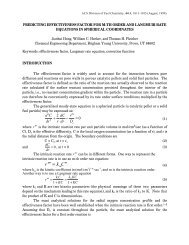
output b[n] is reordered for detection process<strong>in</strong>g to form a 2-D range-azimuth map b(R, θ) as shown <strong>in</strong> Figure 1.<br />
Each column <strong>of</strong> pixels conta<strong>in</strong>s receiver output samples from one transmitter pulse <strong>in</strong>terval. Each time sample n<br />
maps to a correspond<strong>in</strong>g po<strong>in</strong>t <strong>in</strong> space p located at the center <strong>of</strong> a range-azimuth b<strong>in</strong> (or pixel). The midpo<strong>in</strong>t <strong>of</strong><br />
b<strong>in</strong> p has Cartesian coord<strong>in</strong>ates (xp,yp) and polar coord<strong>in</strong>ates (Rp,θp). In expressions where geometrical position<br />
is more mean<strong>in</strong>gful than time sample <strong>in</strong>dex, bp will be used <strong>in</strong>terchangeably with b[n], and serves as a shorthand<br />
notation for b<strong>in</strong> p <strong>in</strong> the range-azimuth map, b(Rp,θp).<br />
<strong>Detection</strong> processor outputs are used both to guide blank<strong>in</strong>g and as <strong>in</strong>puts to the Kalman tracker (see [4]). The<br />
tracker creates detection histories and predicts locations for the next anticipated echoes. These prediction po<strong>in</strong>ts are<br />
utilized <strong>in</strong> turn by the <strong>Bayesian</strong> detector as prior probability <strong>in</strong>puts to adjust detection sensitivity as a function <strong>of</strong><br />
February 22, 2006 DRAFT<br />
Draft manuscript for review, Copyright 2006, American Geophysical Union<br />
2
spatial position.<br />
Sections II and III present the underly<strong>in</strong>g probability models and theoretical algorithm development respectively<br />
for the proposed <strong>Bayesian</strong> detector. Experimental results demonstrat<strong>in</strong>g performance are found <strong>in</strong> Section IV,<br />
followed by conclusions <strong>in</strong> Section V. Prior conference publications provid<strong>in</strong>g partial results are [6] and [7].<br />
II. PROBABILITY MODELS FOR THE BAYESIAN-KALMAN DETECTOR<br />
This section develops statistical models for the prior probability <strong>of</strong> the presence <strong>of</strong> an aircraft radar echo given<br />
the Kalman tracker history. These models will be exploited <strong>in</strong> Section II to form a new algorithm which improves<br />
the probability <strong>of</strong> detect<strong>in</strong>g weak echo pulses for a given fixed rate <strong>of</strong> false alarms. The approach is founded on<br />
fundamental statistical decision theory pr<strong>in</strong>ciples and provides a unified framework for <strong>in</strong>corporat<strong>in</strong>g <strong>in</strong>formation<br />
from a Kalman tracker state space estimate <strong>in</strong>to a constant false alarm rate detector. A new detection statistic, “total<br />
false alarm probability” (PTFA) will be <strong>in</strong>troduced and used as an optimization criterion to derive the algorithm.<br />
The method is general and can be applied to any sequential detection problem possess<strong>in</strong>g a dynamical state space<br />
model suitable for a Kalman tracker. The discussion here however will focus on the application <strong>of</strong> locat<strong>in</strong>g radar<br />
aircraft echoes <strong>in</strong> radio astronomy data.<br />
With<strong>in</strong> a s<strong>in</strong>gle range-azimuth b<strong>in</strong> (Rp,θp) consider the problem <strong>of</strong> decid<strong>in</strong>g whether to accept the hypothesis<br />
that random event Hp: “an aircraft echo is present <strong>in</strong> b<strong>in</strong> p” or its complement ¯ Hp: “no echo is seen <strong>in</strong> b<strong>in</strong> p,”<br />
has occurred. The associated event probabilities are P (Hp) and P ( ¯ Hp) =1− P (Hp). The classical radar detector<br />
makes this decision us<strong>in</strong>g a Neyman-Pearson (N-P) likelihood ratio test by compar<strong>in</strong>g bp with a fixed threshold 1<br />
to achieve maximum probability <strong>of</strong> detection (PD) while enforc<strong>in</strong>g a specified constra<strong>in</strong>t probability <strong>of</strong> false alarm<br />
(PFA) [8]. This is a reasonable approach <strong>in</strong> the usual case when it is difficult to assign mean<strong>in</strong>gful costs to each<br />
decision or when prior probabilities for Hp are unavailable.<br />
However the Kalman track state history conta<strong>in</strong>s <strong>in</strong>formation that can be <strong>in</strong>terpreted, if an appropriate model<br />
can be found, as a prior probability for presence <strong>of</strong> an echo. Echoes are more likely <strong>in</strong> a region S surround<strong>in</strong>g a<br />
po<strong>in</strong>t where the tracker predicts an echo will occur, than <strong>in</strong> the rest <strong>of</strong> the range-azimuth map. The classical Bayes<br />
decision criterion seems a likely candidate to exploit this knowledge, but aga<strong>in</strong> we do not have the required cost<br />
measures <strong>in</strong> our radar detection problem [9]. The proposed algorithm addresses this issue and is structurally related<br />
to both the Bayes and Neyman-Pearson criteria.<br />
A. Kalman Tracker Notation<br />
This section reviews a few equations and notation from [4] which are necessary <strong>in</strong> develop<strong>in</strong>g the <strong>Bayesian</strong><br />
detector. For simplicity the follow<strong>in</strong>g discussion is limited to detections from a s<strong>in</strong>gle track formed by a series<br />
<strong>of</strong> echo detections from one aircraft. However, as implemented the system manages multiple simultaneous tracks.<br />
1When statistics for noise and echo clutter are vary<strong>in</strong>g, a common implementation for constant false alarm rate (CFAR) detection scales the<br />
fixed threshold by a local estimate <strong>of</strong> noise variance. This is effectively a time vary<strong>in</strong>g threshold detector, but does not adjust the threshold<br />
accord<strong>in</strong>g to probability <strong>of</strong> echo presence as does the proposed algorithm.<br />
February 22, 2006 DRAFT<br />
Draft manuscript for review, Copyright 2006, American Geophysical Union<br />
3
Assume the k th radar transmit antenna rotational pass over the radio telescope occurs nom<strong>in</strong>ally at time t[k]. This<br />
yields an aircraft echo detection, referred to as “snapshot k.” All quantities that are updated on a once-per-snapshot<br />
basis will be represented with a [k] argument. For example, the sampled position for a s<strong>in</strong>gle aircraft detected <strong>in</strong><br />
snapshot k is expressed as (R, θ)[k] or (x, y)[k].<br />
The desired tracker outputs at snapshot k are: 1) a prediction po<strong>in</strong>t, (ˆx, ˆy)[k +1|k], where the next detection is<br />
expected, and 2) shape parameters for region S centered on this po<strong>in</strong>t (see Figure 2 and Section II-B). S specifies<br />
an area likely to conta<strong>in</strong> the aircraft echo dur<strong>in</strong>g succeed<strong>in</strong>g snapshot k +1. The “hat” notation, ˆ, will be used<br />
throughout to <strong>in</strong>dicate an estimated or predicted quantity. An argument [k +1|k] <strong>in</strong>dicates a predicted value for<br />
snapshot k +1 based on observations up to and <strong>in</strong>clud<strong>in</strong>g k, while [k|k] <strong>in</strong>dicates a “correction” or smoothed<br />
estimate <strong>of</strong> the true value at time k based on observations through snapshot k. The size <strong>of</strong> S depends on the quality<br />
<strong>of</strong> the track and gets larger with an <strong>in</strong>crease <strong>in</strong> observation noise, missed snapshot detections, or rapid acceleration<br />
<strong>of</strong> the target. S is also used to def<strong>in</strong>e the blanked region for predictive real-time blank<strong>in</strong>g, to determ<strong>in</strong>e which<br />
track each new detection is associated with, and as the boundary for the region <strong>of</strong> <strong>in</strong>creased prior probability for<br />
an arriv<strong>in</strong>g echo pulse used <strong>in</strong> the <strong>Bayesian</strong> detection scheme.<br />
For an exist<strong>in</strong>g track, each new observation snapshot <strong>in</strong>itiates an iteration <strong>of</strong> the Kalman filter which produces<br />
an updated state vector prediction, ˆx[k +1|k], and prediction error covariance matrix P [k +1|k]:<br />
ˆx[k +1|k] = F ˆx[k|k] (1)<br />
P [k +1|k] = FP[k|k]F T + GQG T , where (2)<br />
x[k] =<br />
<br />
x[k] y[k] ˙x[k]<br />
T ˙y[k]<br />
and where x and y are a s<strong>in</strong>gle aircraft’s coord<strong>in</strong>ates, ˙x and ˙y are correspond<strong>in</strong>g velocities, F is the state transition<br />
matrix, G is the process transfer matrix, Q is the process acceleration matrix, and T denotes matrix transpose.<br />
Further details are found <strong>in</strong> [4].<br />
The prediction po<strong>in</strong>t (ˆx, ˆy)[k +1|k] is given by the first two elements <strong>of</strong> ˆx[k +1|k] <strong>in</strong> (1). Its accuracy is gauged<br />
us<strong>in</strong>g P [k +1|k] from (2). With this prior <strong>in</strong>formation, it is reasonable to assume that for the snapshot at time<br />
t[k +1], echo detections have higher probability near the prediction po<strong>in</strong>t.<br />
B. Echo Arrival Probability Model<br />
We propose us<strong>in</strong>g uncerta<strong>in</strong>ty region S as the basis for a spatial prior probability density function (pdf) model<br />
for the presence <strong>of</strong> an aircraft echo <strong>in</strong> snapshot k +1. A few terms must first be def<strong>in</strong>ed before this model can be<br />
<strong>in</strong>troduced.<br />
Assume that for each exist<strong>in</strong>g track exactly one echo will occur (with probability one) dur<strong>in</strong>g snapshot k +1<br />
somewhere <strong>in</strong> an annular slice region<br />
⎧ <br />
⎫<br />
⎨ <br />
x = R cos θ and y = R s<strong>in</strong> θ where ⎬<br />
Ω= (x, y) <br />
⎩ <br />
Rm<strong>in</strong> ≤ R ≤ Rmax, θm<strong>in</strong> ≤ θ ≤ ⎭ θmax<br />
February 22, 2006 DRAFT<br />
Draft manuscript for review, Copyright 2006, American Geophysical Union<br />
4
conta<strong>in</strong><strong>in</strong>g all range-azimuth b<strong>in</strong>s <strong>of</strong> <strong>in</strong>terest. The {(x, y) | expression } notation def<strong>in</strong>es the set <strong>of</strong> all (x, y) pairs<br />
satisfy<strong>in</strong>g the expression. The s<strong>in</strong>gle echo assumption implies that as far as the probability model is concerned, an<br />
established track will always produce an aircraft echo dur<strong>in</strong>g each new antenna pass as long as the track rema<strong>in</strong>s <strong>in</strong><br />
Ω. Cases <strong>of</strong> aircraft dropp<strong>in</strong>g out <strong>of</strong> the airspace due to land<strong>in</strong>g or other events are neglected. These cont<strong>in</strong>gencies<br />
are handled by track management logic which will drop a track after a series <strong>of</strong> snapshots which produce no<br />
detections [4].<br />
Prediction region S is def<strong>in</strong>ed by the quadratic matrix form for an ellipse<br />
S = (x, y) [x − ˆx, y − ˆy]P −1 [x − ˆx, y − ˆy] T ≤ β 2 and (x, y) ∈ Ω <br />
where ∈ denotes “element <strong>of</strong>,” and (ˆx, ˆy) =(ˆx, ˆy)[k +1|k] and P = P [k +1|k] are used with the snapshot<br />
dependence dropped to simplify notation. S is centered on (ˆx, ˆy)[k +1|k] and has size, elongation, and orientation<br />
determ<strong>in</strong>ed by P [k +1|k]. User def<strong>in</strong>ed parameter β controls the scale (size) <strong>of</strong> S relative to the error variances<br />
<strong>in</strong> P .<br />
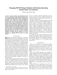
Larger prediction error variance <strong>in</strong> P [k +1|k] leads to a larger S, represent<strong>in</strong>g <strong>in</strong>creased uncerta<strong>in</strong>ty as to where<br />
the next radar echo will be detected. Figure 2 illustrates this behavior. The plot shows track evolution for real GBT<br />
data over five snapshots for a dense scene with multiple overlapp<strong>in</strong>g aircraft tracks. The ellipses represent S for<br />
each established track. Note the variety <strong>of</strong> sizes correspond<strong>in</strong>g to variations <strong>in</strong> track quality.<br />
Due to the assumption <strong>of</strong> a s<strong>in</strong>gle echo per track - per rotational pass <strong>of</strong> the transmit antenna, we can <strong>in</strong>terchangeably<br />
refer to the presence <strong>of</strong> an aircraft or its associated echo. Based on the antenna directional beamwidth<br />
(<strong>in</strong>clud<strong>in</strong>g sidelobes) and the transmit pulse length, shape and repetition rate, this echo spans many range-azimuth<br />
map b<strong>in</strong>s cover<strong>in</strong>g many transmit pulses. Note that <strong>in</strong> this def<strong>in</strong>ition an echo is a collection <strong>of</strong> <strong>in</strong>dividual pulse<br />
returns, not just one pulse reflection. The echo thus has a footpr<strong>in</strong>t F , or region <strong>of</strong> support, due to the effective<br />
po<strong>in</strong>t spread function <strong>in</strong> the range-azimuth map as can be seen <strong>in</strong> Figure 1. This footpr<strong>in</strong>t has fixed size <strong>in</strong> (R, θ)<br />
dependent on transmit beampattern and pulse shape. The echo may or may not be detected <strong>in</strong> any <strong>of</strong> these b<strong>in</strong>s,<br />
depend<strong>in</strong>g on echo amplitude, local noise sample statistics, and the detection algorithm. Figure 4 illustrates the<br />
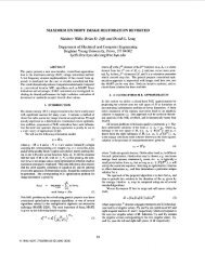
geometry <strong>of</strong> S, F , and a range-azimuth b<strong>in</strong> <strong>in</strong> (R, θ) and (x, y) coord<strong>in</strong>ate systems.<br />
Let fe(x, y | ˆx, ˆy, P ) be the conditional density over (x, y) for the echo footpr<strong>in</strong>t centroid po<strong>in</strong>t (i.e. the actual<br />
aircraft position) given parameters def<strong>in</strong><strong>in</strong>g S. The probability the centroid is conta<strong>in</strong>ed <strong>in</strong> some arbitrary 2-D patch<br />
A is then given by <br />
A fe(x, y | ˆx, ˆy, P )dxdy. We propose the follow<strong>in</strong>g pdf mixture model <strong>in</strong>volv<strong>in</strong>g a truncated<br />
2-D Gaussian term<br />
fe(x, y | ˆx, ˆy, P ) = (4)<br />
⎧<br />
⎪⎨<br />
⎪⎩<br />
1−PS √<br />
CΩ x2 +y2 +<br />
1<br />
2πσ2 |P | exp − 1<br />
2σ2 [x − ˆx, y − ˆy]P −1 <br />
T [x − ˆx, y − ˆy]<br />
1−PS √<br />
CΩ x2 +y2 (x, y) ∈S<br />
(x, y) ∈ ¯ S.<br />
February 22, 2006 DRAFT<br />
Draft manuscript for review, Copyright 2006, American Geophysical Union<br />
5<br />
(3)
The notation ¯ S <strong>in</strong>dicates the complement <strong>of</strong> region S such that Ω=S∪ ¯ S where ∪ is set union. The notation<br />
f(·) will be used throughout the paper to denote any pdf, and subscript e here identifies this as an echo centroid<br />
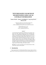
distribution over space. Figure 3 presents an example realization for this pdf.<br />
User def<strong>in</strong>ed parameter σ controls how concentrated fe(x, y | ˆx, ˆy, P ) is around its central peak. The rema<strong>in</strong><strong>in</strong>g<br />
terms <strong>in</strong> (4) are def<strong>in</strong>ed as<br />
<br />
PS =<br />
CΩ =<br />
S<br />
1<br />
2πσ2 |P | exp<br />
<br />
− 1<br />
2σ2 [x − ˆx, y − ˆy]P −1 [x − ˆx, y − ˆy] T<br />
<br />
dxdy (5)<br />
β2<br />
−<br />
=1− e 2σ2 (6)<br />
<br />
Ω<br />
1<br />
dxdy, =<br />
x2 + y2 <br />
=(Rmax − Rm<strong>in</strong>)(θmax − θm<strong>in</strong>)<br />
Ω<br />
where |P | is the matrix determ<strong>in</strong>ant <strong>of</strong> P . Equation (5) was evaluated by substitution <strong>of</strong> (3) for S, us<strong>in</strong>g x = αρ cos θ<br />
and y = ρ s<strong>in</strong> θ, sett<strong>in</strong>g (ˆx, ˆy) =(0, 0), and solv<strong>in</strong>g <strong>in</strong> polar coord<strong>in</strong>ates to obta<strong>in</strong> (6). The probability the echo<br />
centroid is anywhere with<strong>in</strong> S is given by P (HS) = <br />
S fe(x, y |·)dxdy = 1−PS √<br />
S x2 +y2 dxdy + PS ≈ PS. The<br />
approximation is due to the Gaussian term <strong>in</strong> (4) dom<strong>in</strong>at<strong>in</strong>g the expression. Outside <strong>of</strong> S we assume each range-<br />
azimuth b<strong>in</strong> is equally likely to conta<strong>in</strong> the echo centroid. This assumption is made to force a constant threshold,<br />
and thus conventional constant PFA performance outside <strong>of</strong> S <strong>in</strong> the <strong>Bayesian</strong> detection framework <strong>in</strong>troduced <strong>in</strong><br />
the follow<strong>in</strong>g section.<br />
The area <strong>of</strong> a b<strong>in</strong> is proportional to R, which necessitates that over ¯ S, fe(x, y | ˆx, ˆy, P ) must be proportional<br />
to 1/ x 2 + y 2 =1/R. Divid<strong>in</strong>g by CΩ <strong>in</strong> (4) normalizes the <strong>in</strong>tegral to this b<strong>in</strong> area growth with R. Problems<br />
with division by zero are avoided s<strong>in</strong>ce <strong>in</strong> every practical case Rm<strong>in</strong> ≫ 1. Note also that this def<strong>in</strong>ition <strong>in</strong>sures that<br />
<br />
Ω fe(x, y | ˆx, ˆy, P )dxdy =1as required for a pdf.<br />
This model is a reasonable choice because it possesses the follow<strong>in</strong>g necessary characteristics:<br />
dRdθ<br />
• fe(x, y | ˆx, ˆy, P ) decreases monotonically with distance from the prediction po<strong>in</strong>t.<br />
• Over S it is a smooth function with no discont<strong>in</strong>uities.<br />
• The shape <strong>of</strong> fe(x, y | ˆx, ˆy, P ) depends on prediction error covariance, P [k +1|k], such that higher prediction<br />
error leads to lower probability density.<br />
• There is a low, uniform probability across all range-azimuth b<strong>in</strong>s outside the prediction region for presence <strong>of</strong><br />
the echo centroid.<br />
C. Calculat<strong>in</strong>g Prior Probability P ( ¯ Hp)<br />
Given the echo centroid pdf model, fe(x, y | ˆx, ˆy, P ), it is possible to solve for the probability P (Hp) that the<br />
echo footpr<strong>in</strong>t <strong>in</strong>tersects range-azimuth b<strong>in</strong> p.<br />
Let Ap be the 2-D patch which covers b<strong>in</strong> p and which has midpo<strong>in</strong>t (xp,yp) =(Rpcos θp,Rp s<strong>in</strong> θp). Uniform<br />
sampl<strong>in</strong>g <strong>in</strong> Rp and θp yields non uniform spac<strong>in</strong>g <strong>in</strong> (x, y), so the size and orientation <strong>of</strong> Ap depend on Rp and<br />
February 22, 2006 DRAFT<br />
Draft manuscript for review, Copyright 2006, American Geophysical Union<br />
CΩ<br />
6
θp as shown <strong>in</strong> Figure 4, and must be considered when comput<strong>in</strong>g P (Hp). Def<strong>in</strong>e Fq as the footpr<strong>in</strong>t region for an<br />
echo with centroid at another arbitrary b<strong>in</strong> q. All b<strong>in</strong>s q where Fq <strong>in</strong>tersects Ap contribute to the probability P (Hp)<br />
<strong>of</strong> an echo <strong>in</strong> b<strong>in</strong> p. The probability that the echo centroid is <strong>in</strong> b<strong>in</strong> q is given by <br />
Aq fe(x, y | ˆx, ˆy, P )dxdy. Thus<br />
the probability that any portion <strong>of</strong> the echo footpr<strong>in</strong>t is conta<strong>in</strong>ed <strong>in</strong> b<strong>in</strong> p is given by<br />
<br />
<br />
P (Hp) =<br />
fe(x, y | ˆx, ˆy, P )dxdy (7)<br />
{q | Ap∩Fq=φ}<br />
where φ is the empty set and ∩ denotes <strong>in</strong>tersection. Po<strong>in</strong>t (xp,yp) is at the approximate centroid <strong>of</strong> a region ˘ Fp<br />
def<strong>in</strong>ed as the area covered by the union <strong>of</strong> all Fq that satisfy Ap ∩ Fq = φ, i.e. all Fq that overlap Ap.<br />
When ˘ Fp is small 2 compared to S the local surface <strong>of</strong> fe(x, y | ˆx, ˆy, P ) around (xp,yp) is well approximated<br />
by a plane. S<strong>in</strong>ce all b<strong>in</strong> patches Aq <strong>in</strong> this region are approximately the same size as Ap, and the average <strong>of</strong> a<br />
function <strong>of</strong> constant slope over a symmetric planar region is found at its centroid, (7) can be approximated as<br />
<br />
<br />
P (Hp) ≈<br />
fe(x, y | ˆx, ˆy, P )dxdy (8)<br />
where αp = <br />
≈<br />
{q | Ap∩Fq=φ}<br />
<br />
{q | Ap∩Fq=φ}<br />
Aq<br />
Ap<br />
αpfe(xp,yp | ˆx, ˆy, P ) (9)<br />
≈ Kαpfe(xp,yp | ˆx, ˆy, P ) (10)<br />
Ap dxdy is the area <strong>of</strong> patch Ap and K is the number <strong>of</strong> b<strong>in</strong>s, <strong>in</strong>dexed by q, satisfy<strong>in</strong>g {q | Ap ∩Fq =<br />
φ}. The approximations are due to <strong>in</strong>tegrat<strong>in</strong>g over Ap rather than Aq and assum<strong>in</strong>g fe(x, y | ˆx, ˆy, P ) is constant<br />
over small patch Ap <strong>in</strong> (8).<br />
Thus substitut<strong>in</strong>g (4) <strong>in</strong>to (10) yields<br />
⎧<br />
⎪⎨<br />
P (Hp) ≈<br />
⎪⎩<br />
Kαp(1−PS) √<br />
CΩ x2 p +y2 p<br />
+ Kαp<br />
2πσ2 |P | exp − 1<br />
2σ2 [xp − ˆx, yp − ˆy]P −1 <br />
T [xp − ˆx, yp − ˆy]<br />
Kαp(1−PS) √<br />
CΩ x2 p +y2 p<br />
(xp,yp) ∈S<br />
(xp,yp) ∈ ¯ S<br />
P ( ¯ Hp) =1− P (Hp). (12)<br />
The specific pulse repetition and antenna sweep rates <strong>of</strong> the ARSR-3 radar as observed at the GBT, coupled with<br />
our baseband sample rate for b[n], lead to range-azimuth b<strong>in</strong> widths <strong>of</strong> ∆R ≈ 13.87m and ∆θ ≈ 0.0015 radians.<br />
This yields αp ≈ ∆θ∆RRp =0.0208Rp.<br />
2 We have found that ˘ Fp is usually smaller than S <strong>in</strong> practice, due to the short range extent <strong>of</strong> echoes, and particularly when only the transmit<br />
beampattern ma<strong>in</strong>lobe is considered to be part <strong>of</strong> the echo footpr<strong>in</strong>t Fq. Some very bright echoes have sidelobe extent <strong>in</strong> azimuth that could<br />
extend beyond S (see Figure 1), but exclud<strong>in</strong>g these from Fq is reasonable s<strong>in</strong>ce we do not wish to emphasize detection <strong>of</strong> sidelobes <strong>in</strong> any<br />
case.<br />
February 22, 2006 DRAFT<br />
Draft manuscript for review, Copyright 2006, American Geophysical Union<br />
7<br />
(11)
III. BAYESIAN DETECTOR ALGORITHM DEVELOPMENT<br />
This section presents details <strong>of</strong> the proposed improved detection algorithm which is based on a new optimal<br />
detection criterion, “constant total false alarm probability.”<br />
A. <strong>Detection</strong> Statistic Model<br />
The goal <strong>of</strong> radar detection is to observe digital receiver output time series b[n] (equivalently bp) and make a<br />
decision at each time sample (equivalently range-azimuth b<strong>in</strong> p) whether an echo is present. For a s<strong>in</strong>gle b<strong>in</strong> p, bp<br />
is a random variable with conditional amplitude pdf’s fb(bp | ¯ Hp) and fb(bp | Hp), given the absence or presence<br />
<strong>of</strong> an echo respectively. Note that while fe(x, y |·) is a distribution over space, fb(bp |·) describes an amplitude, or<br />
voltage distribution.<br />
Digital receiver output bp is formed as the sum <strong>of</strong> the squares <strong>of</strong> the real (<strong>in</strong> phase) and imag<strong>in</strong>ary (quadrature)<br />
baseband matched filter channels, each <strong>of</strong> which conta<strong>in</strong>s <strong>in</strong>dependent additive Gaussian noise [10]. As such, bp<br />
consists <strong>of</strong> the sum <strong>of</strong> two squared Gaussian random variables, so bp/ση (where σ 2 η is the noise variance for both<br />
the real or imag<strong>in</strong>ary channels) has a central chi-squared (χ 2 2) distribution with two degrees <strong>of</strong> freedom under ¯ H,<br />
and noncentral χ 2 2 under H as illustrated <strong>in</strong> Figure 5 [8][11]. In many communications texts vp = bp is used as<br />
the detection statistic, and it is shown to have a Rice distribution,<br />
<br />
vp|s|<br />
fv(vp|Hp) = vp<br />
σ2 I0<br />
η<br />
σ 2 η<br />
<br />
e − v2 p +s2<br />
2σ2 η<br />
where I0(·) is the zero-th order modified Bessel function <strong>of</strong> the first k<strong>in</strong>d and noncentrality parameter s is<br />
proportional to echo signal power [10]. The follow<strong>in</strong>g discussion uses bp as the detection statistic, but a parallel<br />
development could also be presented us<strong>in</strong>g vp by simply tak<strong>in</strong>g the square root <strong>of</strong> each side <strong>of</strong> every threshold test<br />
<strong>in</strong>equality.<br />
B. Related Detector Structures<br />
This section discusses some well known detector architectures as a brief tutorial background and to motivate<br />
design choices for the new method. The <strong>in</strong>tent is to show that the <strong>Bayesian</strong> constant PTFA detector <strong>in</strong>troduced <strong>in</strong><br />
equations (19) - (21) below can be <strong>in</strong>terpreted as a natural extension <strong>of</strong> familiar concepts.<br />
The famous Neyman-Pearson (N-P) detector uses the follow<strong>in</strong>g likelihood ratio test:<br />
fb(bp | Hp)<br />
fb(bp | ¯ Hp)<br />
where the stacked <strong>in</strong>equality denotes “decide Hp if the left hand side is greater than τ ′ NP , otherwise choose ¯ Hp.”<br />
S<strong>in</strong>ce the likelihood ratio is monotonic <strong>in</strong> b for these particular pdf’s, (13) is equivalent to a simple direct threshold<strong>in</strong>g<br />
<strong>of</strong> the receiver output:<br />
bp<br />
H<br />
><br />
< ¯H<br />
February 22, 2006 DRAFT<br />
Draft manuscript for review, Copyright 2006, American Geophysical Union<br />
H<br />
><br />
< ¯H<br />
τ NP<br />
τ ′ NP<br />
8<br />
(13)<br />
(14)
where τ NP is a function <strong>of</strong> the constant threshold τ ′ NP . The associated probability <strong>of</strong> false alarm (detect<strong>in</strong>g an echo<br />
when none is present) is def<strong>in</strong>ed as<br />
PFA =<br />
∞<br />
τ NP<br />
fb(bp | ¯ Hp)db. (15)<br />
The usual approach for establish<strong>in</strong>g the threshold level is to fix PFA to some suitably small constant and then solve<br />
(15) for τ NP. Note that PFA is def<strong>in</strong>ed conditionally under ¯ H and that the <strong>in</strong>tegrand comes from the denom<strong>in</strong>ator<br />
<strong>of</strong> the left hand side <strong>of</strong> (13).<br />
The simple NP test does not provide a mechanism for exploit<strong>in</strong>g prior probability <strong>in</strong>formation obta<strong>in</strong>ed from the<br />
tracker. One possible alternative is the Bayes decision criterion [9] [12]<br />
P (Hp) fb(bp | Hp)<br />
P ( ¯ Hp) fb(bp | ¯ Hp)<br />
H<br />
><br />
< ¯H<br />
CH, H¯ − CH, ¯ H¯<br />
CH,H ¯ − CH,H<br />
= τ(C) (16)<br />
where constants CI,J for I,J ∈{ ¯ H,H} are costs (also called Bayes loss) associated with decid<strong>in</strong>g I when J<br />
is true, and C = {C ¯ H, ¯ H,C¯ H,H,C 1, ¯ H,CH,H}. Unfortunately, (16) has some disadvantages. We do not have a<br />
satisfactory systematic approach to specify the costs. Also it is not clear how to frame this <strong>in</strong> the desired direct<br />
threshold<strong>in</strong>g form <strong>of</strong> (14).<br />
To illustrate the difficulty, note that the left hand side <strong>of</strong> (16) is still monotonic <strong>in</strong> bp and that τ(C) is a constant<br />
(though dependent on C). This suggests that a correspond<strong>in</strong>g threshold test comparable to (13) would be<br />
fb(bp | Hp)<br />
fb(bp | ¯ Hp)<br />
H<br />
><br />
< ¯H<br />
P ( ¯ Hp)<br />
τ(C) =τ(p, C). (17)<br />
P (Hp)<br />
Now threshold τ(p, C) depends on position p s<strong>in</strong>ce P ( ¯ Hp) and P (Hp) are spatially vary<strong>in</strong>g. In this <strong>Bayesian</strong><br />
framework the direct threshold form correspond<strong>in</strong>g to (14) is found by def<strong>in</strong><strong>in</strong>g the likelihood ratio function L(b) =<br />
fb(b | Hp)/fb(b | ¯ Hp) and operat<strong>in</strong>g on the left and right hands sides <strong>of</strong> (17) with the functional <strong>in</strong>verse L −1 (·) to<br />
obta<strong>in</strong><br />
bp<br />
H<br />
><br />
< ¯H<br />
L −1 τ(p, C) = τ ′ (p, C). (18)<br />
The problem with this formulation is that although it is <strong>in</strong> fact the desired direct test on receiver output sample bp,<br />
we do not know how to evaluate threshold τ ′ (p, C). In a typical scenario all the CI,J are unknown. Also L −1 (·)<br />
depends on fb(τ(p, C) | Hp) which unlike fb(τ(p, C) | ¯ Hp) is hard to model because aircraft echoes have unknown<br />
random <strong>in</strong>tensities. One cannot readily f<strong>in</strong>d the appropriate threshold value because we cannot use the constant<br />
PFA constra<strong>in</strong>t <strong>of</strong> (15) to avoid these complexities and still satisfy the desired <strong>Bayesian</strong> relationships <strong>of</strong> (16).<br />
C. Constant PTFA <strong>Detection</strong><br />
We propose an alternative <strong>Bayesian</strong> framework for improved detection performance to address the problems<br />
mentioned above, and which is based on a physically mean<strong>in</strong>gful criterion related to specify<strong>in</strong>g a fixed PFA.We<br />
February 22, 2006 DRAFT<br />
Draft manuscript for review, Copyright 2006, American Geophysical Union<br />
9
def<strong>in</strong>e the unconditional “total probability <strong>of</strong> false alarm” (PTFA) as the jo<strong>in</strong>t probability that a spatially vary<strong>in</strong>g<br />
threshold, τp, was crossed and no echo was present,<br />
PTFA = P ((bp >τp) ∩ ¯ Hp)<br />
∞<br />
= P ( ¯ Hp) fb(b | ¯ Hp) db (19)<br />
τp<br />
= P ( ¯ Hp)PFA.<br />
This is the total probability (i.e. not conditioned on H or ¯ H) that a false alarm will occur at range-azimuth b<strong>in</strong> p<br />
given some τp.<br />
Equation (19) provides a means to solve for an appropriate threshold for a direct test <strong>in</strong> the form <strong>of</strong> (14) or(18),<br />
but which <strong>in</strong>corporates the prior <strong>in</strong>formation P ( ¯ Hp) drawn from the Kalman track history through equations (11)<br />
and (12). Note that τp = τ ′ (p, C) = τ NP so the detector is neither N-P, nor classical Bayes decision criterion, but<br />
depends on the Bayes relationship used <strong>in</strong> (19).<br />
Spatially vary<strong>in</strong>g τp is found by specify<strong>in</strong>g a fixed value for the acceptable PTFA and solv<strong>in</strong>g (19) for τp <strong>in</strong><br />
closed form:<br />
τp = −σ 2 <br />
PTFA<br />
η log<br />
P ( ¯ <br />
Hp)<br />
where PTFA is specified by the user to be some small constant, P ( ¯ Hp) is given by (11) and (12), and 2σ 2 η is the<br />
complex noise variance for b[n].<br />
This is not the same test as <strong>in</strong> (16). One obvious dist<strong>in</strong>ction is that costs Ci,j are not <strong>in</strong>cluded s<strong>in</strong>ce the threshold<br />
is set by solv<strong>in</strong>g a PTFA equation. Some <strong>in</strong>sight is provided by not<strong>in</strong>g that (19) uses the left hand side denom<strong>in</strong>ator<br />
<strong>of</strong> (16) as an <strong>in</strong>tegrand, just as (15) <strong>in</strong>tegrates the denom<strong>in</strong>ator <strong>of</strong> (13). Also, we propose that constant PTFA<br />
detection is a rational solution given that the expected total number <strong>of</strong> false alarms will be known over the range<br />
azimuth map. This is set as a design parameter. On the other hand, a fixed PFA detector will have vary<strong>in</strong>g numbers<br />
<strong>of</strong> false alarms as P ( ¯ H) varies. The computational load for a radar detection system is proportional to the number<br />
<strong>of</strong> threshold cross<strong>in</strong>gs, so be<strong>in</strong>g able to fix the average number <strong>of</strong> false alarms can be a useful constra<strong>in</strong>t on system<br />
capacity.<br />
Summariz<strong>in</strong>g, the constant PTFA detector (CTFA) is computed with the follow<strong>in</strong>g steps:<br />
1) Set PTFA = a small constant.<br />
2) Evaluate (20) to f<strong>in</strong>d the spatially vary<strong>in</strong>g τp at each range-azimuth b<strong>in</strong>, b(xp,yp).<br />
3) Threshold each b<strong>in</strong>:<br />
bp<br />
H<br />
><br />
< ¯H<br />
10<br />
(20)<br />
τp. (21)<br />
The effect <strong>of</strong> this approach is that the threshold is lowered <strong>in</strong> the prediction regions S where based on prior track<br />
history it is known that echoes are more likely. This leads to more reliable detection <strong>of</strong> weak aircraft echoes. By<br />
proper selection <strong>of</strong> parameters PTFA, β, and σ, the probability <strong>of</strong> detection PD = ∞<br />
τp fb(bp|Hp) is <strong>in</strong>creased while<br />
February 22, 2006 DRAFT<br />
Draft manuscript for review, Copyright 2006, American Geophysical Union
false alarms are kept low, as shown <strong>in</strong> Figure 5. Figure 6 illustrates the variable threshold τp plotted as a function<br />
<strong>of</strong> x and y for two prediction regions from two tracks. Note that the lower quality track has a wider prediction<br />
region (right), lead<strong>in</strong>g to a more shallow threshold depression. This corresponds to greater uncerta<strong>in</strong>ty about the<br />
next echo location, so less emphasis on detection is generated here. Note however that <strong>in</strong> both cases the threshold<br />
reduction is relatively small (less than 0.5% <strong>in</strong> this example) as a natural consequence <strong>of</strong> the way the constant<br />
PTFA detector is def<strong>in</strong>ed. However, s<strong>in</strong>ce it is applied over many b<strong>in</strong>s, even such a small change <strong>in</strong> threshold can<br />
have a significant effect on detection statistics, improv<strong>in</strong>g the probability <strong>of</strong> f<strong>in</strong>d<strong>in</strong>g a threshold cross<strong>in</strong>g <strong>in</strong> at least<br />
one b<strong>in</strong> <strong>of</strong> the echo footpr<strong>in</strong>t. This is demonstrated <strong>in</strong> results presented <strong>in</strong> the follow<strong>in</strong>g section. With this small<br />
threshold depression PD is <strong>in</strong>creased while avoid<strong>in</strong>g the potential problem <strong>of</strong> forc<strong>in</strong>g a detection <strong>in</strong> S whether an<br />
echo is present or not.<br />
As noted earlier there are <strong>of</strong>ten multiple concurrent aircraft tracks <strong>in</strong> Ω, each with a prediction region and<br />
associated computed threshold levels τp. This potential conflict is handled as follows. Let τp,j be the threshold<br />
computed for the p th range-azimuth b<strong>in</strong> us<strong>in</strong>g Sj from the j th track. A s<strong>in</strong>gle threshold test is made for each b<strong>in</strong><br />
as <strong>in</strong> (21) where<br />
τp = m<strong>in</strong> τp,j. (22)<br />
j<br />
This method was used <strong>in</strong> Figure 6. The set <strong>of</strong> threshold cross<strong>in</strong>gs is then processed with the CLEAN algorithm<br />
[13] to collapse the sidelobe structure to a s<strong>in</strong>gle po<strong>in</strong>t, and each cleaned detection is assigned to an exist<strong>in</strong>g or<br />
new track follow<strong>in</strong>g arbitration rules described <strong>in</strong> [4].<br />
A. Performance Evaluation with Simulated Data<br />
IV. EXPERIMENTAL RESULTS<br />
It is very difficult to quantitatively characterize detection performance us<strong>in</strong>g real-world data because relevant<br />
signal properties such as signal to noise ratio (SNR) and absence or presence <strong>of</strong> an echo are unknown. We have<br />
developed a realistic echo synthesis code to generate data used <strong>in</strong> Monte Carlo simulation trials to estimate detection<br />
properties such as probability <strong>of</strong> detection (PD) and probability <strong>of</strong> false alarm (PFA) as functions <strong>of</strong> SNR and<br />
aircraft motion dynamics. The new <strong>Bayesian</strong> detector is shown to improve PD for a fixed PFA as compared with<br />
the conventional approach, thus validat<strong>in</strong>g the strategy <strong>of</strong> detector design based on constant PTFA.<br />
The simulator generates a time sequence b[n] <strong>of</strong> receiver outputs with the follow<strong>in</strong>g properties:<br />
• Receiver sensitivity, IF bandwidth, data sample rate, and antenna sidelobe ga<strong>in</strong> response all approximately<br />
match those used to collect radar data at the GBT.<br />
• Transmitter pulse length, pulse shape, pulse repetition rate, antenna sweep rate, and transmit beamwidth<br />
approximate those <strong>of</strong> the ARSR-3 radar system as discussed <strong>in</strong> [14], [15], [5], [4].<br />
• Additive white Gaussian noise (AWGN) is used with variance ση 2 match<strong>in</strong>g sample variance estimated from<br />
real radar-echo-free GBT data.<br />
• In order to elim<strong>in</strong>ate problems <strong>in</strong> associat<strong>in</strong>g new detections with their correspond<strong>in</strong>g tracks, there is only one<br />
simulated echo track <strong>in</strong> each randomly generated trial observation.<br />
February 22, 2006 DRAFT<br />
Draft manuscript for review, Copyright 2006, American Geophysical Union<br />
11
• Realistic aircraft motion is simulated us<strong>in</strong>g the Kalman state space model with acceleration a(k) generated<br />
as a lowpass filtered 2-D Gaussian i.i.d. random noise process. The lowpass corner frequency is adjusted to<br />
produce smoothly connected random maneuvers with turn radii consistent with commercial aircraft.<br />
• The pulse echo amplitude follows a Swirl<strong>in</strong>g IV distribution model suitable for a square law receiver [16].<br />
Received pulses have constant mean amplitude throughout an entire scan, but are uncorrelated from pulse to<br />
pulse. The echo amplitude pdf is given by<br />
fΣ(σ) = 4σ<br />
σ2 exp(−<br />
av<br />
2σ<br />
) (23)<br />
σav<br />
where subscript Σ denotes the Swirl<strong>in</strong>g pdf, σ is the random radar cross section (RCS) value, and σav is the<br />
average RCS over all target fluctuations.<br />
A Monte-Carlo simulation was used with repeated random trials to evaluate PD vs. PFA <strong>in</strong> order to estimate the<br />
receiver operat<strong>in</strong>g characteristic (ROC). When compar<strong>in</strong>g the new <strong>Bayesian</strong> algorithm with a conventional detector<br />
one must carefully consider the differences <strong>in</strong> how false alarms arise. As def<strong>in</strong>ed <strong>in</strong> (15), PFA only depends on the<br />
noise power and a threshold τNP with fixed value over the entire range-azimuth map. However, the new algorithm<br />
improves PD at the cost <strong>of</strong> a slight local false alarm rate <strong>in</strong>crease <strong>in</strong>side S. To be fair, a comparison <strong>of</strong> PD between<br />
algorithms must be made when each has the same effective total PFA value. For Figure 7 the “Probability <strong>of</strong> False<br />
Alarm” values along the horizontal axis represent actual observed error counts across a series <strong>of</strong> range-azimuth map<br />
random realizations, divided by the number <strong>of</strong> trials and the number <strong>of</strong> b<strong>in</strong>s (pixels) <strong>in</strong> a map. In order to calculate<br />
sample statistics <strong>in</strong> the realistic PFA regime between 10 −8 and 10 −6 it was necessary to run many thousands<br />
<strong>of</strong> random trials to observe enough <strong>of</strong> the rare false alarms to keep error variance low. A family <strong>of</strong> ROC curves<br />
is presented to demonstrate the superior performance <strong>of</strong> the new algorithm. <strong>Detection</strong> probabilities are uniformly<br />
higher for the <strong>Bayesian</strong> detector when both algorithms are produc<strong>in</strong>g the same number <strong>of</strong> false alarms.<br />
B. Performance with Real Data<br />
Two sets <strong>of</strong> real data were recorded at the GBT and used to test performance <strong>of</strong> the echo detection algorithm,<br />
track<strong>in</strong>g, and blank<strong>in</strong>g. Set one consists <strong>of</strong> five 12 second long data w<strong>in</strong>dows recorded at one m<strong>in</strong>ute <strong>in</strong>tervals on<br />
April 5, 2002. Set two conta<strong>in</strong>s a cont<strong>in</strong>uous block <strong>of</strong> 10 m<strong>in</strong>utes <strong>of</strong> data (50 radar antenna rotations) recorded <strong>in</strong><br />
January, 2003. The Kalman tracker and both the conventional N-P and new <strong>Bayesian</strong> detectors were run on all data<br />
<strong>in</strong> both sets. A more extensive presentation <strong>of</strong> these results is found <strong>in</strong> [5].<br />
In data set one there are five snapshots conta<strong>in</strong><strong>in</strong>g eight dist<strong>in</strong>ct aircraft tracks. The <strong>Bayesian</strong> detector found<br />
three echoes that were missed by the conventional method. A missed detection was declared when no conventional<br />
threshold cross<strong>in</strong>g occurred <strong>in</strong> a track’s prediction region at snapshot t[k +1], but was reacquired <strong>in</strong> snapshot<br />
t[k +2], i.e. the tracker had to make a two-step prediction update to keep the track alive. The reacquisition at<br />
t[k +2] implies that the aircraft echo was present <strong>in</strong> S at t[k +1], but was just too weak to detect. In total there<br />
were 33 track associated detections with the conventional algorithm, and 36 with the new detector. No “false alarm”<br />
detections (i.e. new threshold cross<strong>in</strong>gs not associated with a track) arose with the new method.<br />
February 22, 2006 DRAFT<br />
Draft manuscript for review, Copyright 2006, American Geophysical Union<br />
12
In data set two there were four missed detections recovered by the <strong>Bayesian</strong> algorithm over 15 snapshots with<br />
six active tracks as shown <strong>in</strong> Figure 8. One more possible false alarm was made by the <strong>Bayesian</strong> detector than with<br />
the N-P approach. For this experiment both PFA and PTFA were set to 3.87 × 10⁻⁸ when calculat<strong>in</strong>g threshold<br />
sett<strong>in</strong>gs.<br />
On the other hand, Figure 9 illustrates what occurs when the N-P detection threshold is lowered (by <strong>in</strong>creas<strong>in</strong>g<br />
the design PFA) <strong>in</strong> an attempt to recover the lost echoes which were found by the <strong>Bayesian</strong> detector. When PFA is<br />
raised from 3.87 × 10⁻⁸ to 2.32 × 10⁻⁷ two <strong>of</strong> the four miss<strong>in</strong>g detections were found, but four false alarms were<br />
added. In order to detect the rema<strong>in</strong><strong>in</strong>g two echoes PFA had to be raised so high that hundreds <strong>of</strong> false alarms<br />
appeared (not shown <strong>in</strong> this figure). Clearly the <strong>Bayesian</strong> approach provides better false alarm management while<br />
improv<strong>in</strong>g weak echo detection.<br />
To illustrate the potential scientific observational impact <strong>of</strong> blank<strong>in</strong>g the previously missed echoes which are now<br />
caught by the <strong>Bayesian</strong> algorithm we processed a segment <strong>of</strong> data from data set two. This w<strong>in</strong>dow from 187.2 to<br />
188.4 seconds <strong>in</strong> the record<strong>in</strong>g produced no aircraft detections us<strong>in</strong>g the conventional algorithm, but the new method<br />
found three. Figure 10 shows power spectral estimates accumulated over the 1.2 second w<strong>in</strong>dow which conta<strong>in</strong>ed<br />
ground terra<strong>in</strong> echo clutter. The upper curve <strong>in</strong>cludes no radar pulse blank<strong>in</strong>g and exhibits a dom<strong>in</strong>ant spectral peak<br />
around 5.5 MHz caused by ground clutter. The lower curve shows the spectrum after fixed time w<strong>in</strong>dow blank<strong>in</strong>g<br />
synchronized to the transmit antenna sweep. This corresponds to excis<strong>in</strong>g all data between a delay <strong>of</strong> 0 and 150<br />
µs <strong>in</strong> Figure 1. At this plott<strong>in</strong>g scale all RFI appears to have been elim<strong>in</strong>ated. All blank<strong>in</strong>g was implemented by<br />
“zero-stuff<strong>in</strong>g” [3], that is, plac<strong>in</strong>g zeros <strong>in</strong>to the time samples where radar <strong>in</strong>terference is detected.<br />
However, at the expanded scale <strong>of</strong> Figure 11, a difference is seen between spectral estimates us<strong>in</strong>g the new<br />
<strong>Bayesian</strong> detection as compared with conventional N-P detection. The Kalman track was established from five<br />
previous antenna sweeps, which occur at 12 s <strong>in</strong>tervals. The three weak aircraft echoes which were detected<br />
with the new algorithm were blanked, and the result<strong>in</strong>g lower curve spectrum shows reduced bias near 5.5 MHz<br />
correspond<strong>in</strong>g to the radar pulse center frequency.<br />
V. CONCLUSIONS<br />
The forgo<strong>in</strong>g analysis has demonstrated the potential for a Kalman tracker based <strong>Bayesian</strong> detector to provide<br />
high performance pulsed <strong>in</strong>terference removal from radio astronomical data. Even when result<strong>in</strong>g spectral estimates<br />
are improved only subtly, it is desirable <strong>in</strong> radio astronomy to remove every <strong>in</strong>terference component possible to<br />
<strong>in</strong>crease confidence <strong>in</strong> the affected scientific observation. These radar systems are not go<strong>in</strong>g away, and as <strong>in</strong>terest<br />
<strong>in</strong>creases for deep space observation <strong>in</strong> the radar band allocations such a system will become <strong>in</strong>creas<strong>in</strong>gly necessary.<br />
Though the mathematical development presented here appears fairly complex, computer implementation <strong>of</strong> the<br />
tracker - constant PTFA detector is quite straightforward. Computational burdens are small because track state<br />
and threshold computation updates need be made only once per 12 second antenna sweep. Thus, aside from the<br />
digital receiver functions, only modest computational resources are required as long as a digitized signal stream<br />
is available. The digital radar receiver must operate at RF sample rates, but such systems are <strong>in</strong> widespread use.<br />
February 22, 2006 DRAFT<br />
Draft manuscript for review, Copyright 2006, American Geophysical Union<br />
13
Any system used to blank pulses after detect<strong>in</strong>g them (e.g. us<strong>in</strong>g N-P detection) must use the same type digital<br />
radar receiver front-end. Therefore, by comparison the additional computational burden to add Kalman track<strong>in</strong>g and<br />
constant PTFA detection could be handled by the slowest <strong>of</strong> PC’s.<br />
This study suggests that the Kalman tracker <strong>Bayesian</strong> detector system is a good candidate for real-time operation<br />
and permanent implementation at the observatory. Plans are currently under consideration to pursue fund<strong>in</strong>g for<br />
such an obvious next step.<br />
However, even without <strong>in</strong>vest<strong>in</strong>g <strong>in</strong> significant real-time process<strong>in</strong>g resources the proposed system can be used<br />
<strong>in</strong> a post process<strong>in</strong>g mode on virtually any extended pre-recorded data set conta<strong>in</strong><strong>in</strong>g pulsed radar RFI. In a post<br />
process<strong>in</strong>g scenario it would also be possible to adapt the proposed approach to operate both backwards and forwards<br />
<strong>in</strong> time. One can envision a forward-backward two pass echo Kalman track<strong>in</strong>g scheme and a <strong>Bayesian</strong> detector<br />
which draws on the entire data set (rather than just past detections) for prior probability <strong>in</strong>ference. This should<br />
<strong>of</strong>fer additional detection performance ga<strong>in</strong>s, particularly at the beg<strong>in</strong>n<strong>in</strong>g <strong>of</strong> an aircraft track where start-up errors<br />
are large. As described above, two successive N-P detections are required before a track can be <strong>in</strong>itiated. Us<strong>in</strong>g<br />
backward prediction it would be possible to f<strong>in</strong>d weak echoes which did not cross the N-P threshold and which<br />
occurred before the causal track was created. Future research plans <strong>in</strong>clude develop<strong>in</strong>g this bidirectional track<strong>in</strong>g<br />
detector. Block estimation methods that do not rely on sequential process<strong>in</strong>g, either forward or backward, can also<br />
be <strong>in</strong>vestigated.<br />
REFERENCES<br />
[1] S. Ell<strong>in</strong>gson and G. Hampson, “Rfi and asynchronous pulse blank<strong>in</strong>g <strong>in</strong> the 1230-1375 mhz band at arecibo,” Ohio State University, Tech.<br />
Rep. 743467-3, 2003.<br />
[2] S. Ell<strong>in</strong>gson, “Capabilities and limitations <strong>of</strong> adaptive cancel<strong>in</strong>g for microwave radiometry,” IEEE International Geoscience and Remote<br />
Sens<strong>in</strong>g Symposium 2002, IGARSS’02, vol. 3, pp. 1685–1687, June 2002.<br />
[3] Q. Zhang, Y. Zheng, S. Wilson, J. Fisher, and R. Bradley, “Combat<strong>in</strong>g pulsed radar <strong>in</strong>terference <strong>in</strong> radio astronomy,” The Astronomical<br />
Journal, vol. 126, pp. 1588–1594, 2003.<br />
[4] W. Dong, B. Jeffs, and J. Fisher, “<strong>Radar</strong> <strong>in</strong>terference blank<strong>in</strong>g <strong>in</strong> radio astronomy us<strong>in</strong>g a kalman tracker,” <strong>Radio</strong> Science, RS5S04,<br />
doi:10.1029/2004RS003130, vol. 40, no. 5, June 2005.<br />
[5] W. Dong, “Time blank<strong>in</strong>g for gbt data with radar rfi,” Master’s thesis, Brigham Young University, 2004.<br />
[6] W. Dong, B. Jeffs, and J. Fisher, “A kalman-tracker-based bayesian detector for radar <strong>in</strong>terference <strong>in</strong> radio astronomy,” <strong>in</strong> Proc. <strong>of</strong> the<br />
IEEE International Conf. on Acoust,, Speech, and Signal Process<strong>in</strong>g, vol. IV, 2005, pp. 657–660.<br />
[7] W. Dong and B. Jeffs, “Kalman track<strong>in</strong>g and bayesian detection for radar rfi blank<strong>in</strong>g,” <strong>in</strong> Proceed<strong>in</strong>gs <strong>of</strong> RFI2004, IUCAD DRAO<br />
Workshop <strong>in</strong> Mitigation <strong>of</strong> <strong>Radio</strong> Frequency <strong>Interference</strong> <strong>in</strong> <strong>Radio</strong> <strong>Astronomy</strong>, Web address:<br />
http://www.ece.vt.edu/∼swe/RFI2004/, Penticton, British Columbia, July 2004.<br />
[8] H. V. Trees, <strong>Detection</strong>, Estimation, and Modulation Theory, Part III, <strong>Radar</strong>-Sonar Signal Process<strong>in</strong>g and Gaussian Signals <strong>in</strong> Noise. John<br />
Wiley and Sons, 2001.<br />
[9] ——, <strong>Detection</strong>, Estimation, and Modulation Theory, Part I. John Wiley and Sons, 2001.<br />
[10] J. Proakis and M. Salehi, Communications Systems Eng<strong>in</strong>eer<strong>in</strong>g, Second Ed. Englewood Cliffs, New Jersey: Prentice Hall, 2002.<br />
[11] A. Papoulis, Probability, Random Variables, and Stochastic Processes, Second Ed. New-York: McGraw Hill, 1984.<br />
[12] L. L. Scharf, Statistical Signal Process<strong>in</strong>g: <strong>Detection</strong>, Estimation, and Time Series Analysis. Read<strong>in</strong>g, Massachusetts: Addison-Wesley,<br />
1991.<br />
[13] J. Högbom, “Aperture synthesis with a nonregular distribution <strong>of</strong> <strong>in</strong>terferometer basel<strong>in</strong>es,” <strong>Astronomy</strong> and Astrophysics Supplement, vol. 15,<br />
pp. 417–426, 1974.<br />
February 22, 2006 DRAFT<br />
Draft manuscript for review, Copyright 2006, American Geophysical Union<br />
14
[14] J. Fisher, “Summary <strong>of</strong> rfi data samples at green bank,” National <strong>Radio</strong> <strong>Astronomy</strong> Observatory, Green Bank Observatory, Tech. Rep.,<br />
2001.<br />
[15] ——, “Analysis <strong>of</strong> radar data from february 6, 2001,” National <strong>Radio</strong> <strong>Astronomy</strong> Observatory, Green Bank Observatory, Tech. Rep., 2001.<br />
[16] B. Mahafza, <strong>Radar</strong> Systems Analysis and Design Us<strong>in</strong>g MATLAB. Chapman and Hall/CRC Press, 2000.<br />
February 22, 2006 DRAFT<br />
Draft manuscript for review, Copyright 2006, American Geophysical Union<br />
15
Pulse delay <strong>in</strong> microseconds / range R <strong>in</strong> km<br />
900 /<br />
270<br />
600 /<br />
180<br />
300 /<br />
90<br />
0 / 0<br />
1 / -18 1.5 / -8 2 / 2 2.5 / 12 3 / 22 3.5 / 32<br />
Antenna sweep time <strong>in</strong> seconds / Azimuth θ <strong>in</strong> degrees<br />
Fig. 1. A typical range-azimuth map, b(R, θ), <strong>of</strong> radar data collected at the GBT. This map covers approximately 60◦ <strong>of</strong> azimuth θ along<br />
the 3.5 s span <strong>of</strong> the horizontal axis. The bright region at about 1.8 seconds and 0-100 µs delay corresponds to the transmitter beam pass<strong>in</strong>g<br />
overhead at the GBT and generat<strong>in</strong>g strong reflections from nearby mounta<strong>in</strong> peaks. Several aircraft echoes are visible. Note the horizontal<br />
extent <strong>of</strong> the bright echoes due to the sidelobe directional response pattern <strong>of</strong> the radar transmit antenna. The echo extent or region <strong>of</strong> support<br />
for a s<strong>in</strong>gle aircraft is denoted as footpr<strong>in</strong>t F .<br />
February 22, 2006 DRAFT<br />
Draft manuscript for review, Copyright 2006, American Geophysical Union<br />
16
y (meter)<br />
x x−y 104<br />
9<br />
8<br />
7<br />
6<br />
5<br />
4<br />
3<br />
coord<strong>in</strong>ate<br />
−3 −2.5 −2 −1.5 −1 −0.5 0 0.5 1 1.5 2<br />
x 10 4<br />
2<br />
detection<br />
prediction<br />
estimation<br />
x (meter)<br />
Fig. 2. An example <strong>of</strong> Kalman track<strong>in</strong>g performance for data acquired at the GBT. Four aircraft tracks have been automatically established<br />
and plotted, <strong>in</strong>clud<strong>in</strong>g a pair <strong>of</strong> cross<strong>in</strong>g tracks. Data from five snapshots are shown. In order to exaggerate the motion between snapshots and<br />
reduce computational demand, only every other antenna pass was used, result<strong>in</strong>g <strong>in</strong> a snapshot <strong>in</strong>terval ≈ 24s. The f<strong>in</strong>al po<strong>in</strong>t plotted for each<br />
track is the prediction po<strong>in</strong>t, (ˆx, ˆy)[k +1|k]. Prediction regions, S, shown by the dashed ellipses vary <strong>in</strong> size accord<strong>in</strong>g to track quality. Note<br />
that the center track has a large S due to a missed detection. The entire area covered by the figure is represented by Ω. Predictive real-time<br />
blank<strong>in</strong>g is accomplished by excis<strong>in</strong>g the prediction region data. For this example, <strong>of</strong>f diagonal terms <strong>in</strong> P [k +1|k] were assumed to be zero,<br />
which forces the S ellipses to align to the x and y axes.<br />
February 22, 2006 DRAFT<br />
Draft manuscript for review, Copyright 2006, American Geophysical Union<br />
17
fe(x,y| . )<br />
0.02<br />
0.015<br />
0.01<br />
0.005<br />
0<br />
10<br />
5<br />
y<br />
0<br />
S<br />
5<br />
10<br />
10<br />
5<br />
0<br />
(xp,yp)<br />
Fig. 3. A typical realization <strong>of</strong> the two dimensional Gaussian model for fe(x, y | ˆx, ˆy, P ) both <strong>in</strong>side and outside elliptical region S. (xp,yp)<br />
is an arbitrary po<strong>in</strong>t <strong>in</strong>side S. The x, y scale <strong>of</strong> this plot is centered relative to an arbitrary (ˆx, ˆy)<br />
February 22, 2006 DRAFT<br />
Draft manuscript for review, Copyright 2006, American Geophysical Union<br />
x<br />
5<br />
10<br />
18
y<br />
∆R<br />
S<br />
∆θ<br />
x<br />
(x,y)<br />
(xq,yq)<br />
(x 1 ,y 1 )<br />
(R 1 ,θ 1 )<br />
ry<br />
(xp,yp)<br />
(Rp,θp)<br />
Fig. 4. Geometry <strong>of</strong> a prediction region, S centered on (ˆx, ˆy). r 2 x = β 2 P11[k +1|k] and r 2 y = β 2 P22[k +1|k] where Pij[k +1|k] is the<br />
i, j-th matrix element <strong>in</strong> P [k +1|k]. M<strong>in</strong>or axis length and rotation <strong>of</strong> the ellipse are affected by <strong>of</strong>f diagonal term P12[k +1|k]. Ap covers<br />
the range-azimuth b<strong>in</strong> centered on (xp,yp). Fq is the echo footpr<strong>in</strong>t for an echo centered on some other b<strong>in</strong>, q. Due to uniform sampl<strong>in</strong>g <strong>in</strong><br />
angle with spac<strong>in</strong>g ∆θ and because Rp >R1, the area <strong>of</strong> b<strong>in</strong> Ap is greater than that <strong>of</strong> the b<strong>in</strong> centered on (x1,y1). Note that the sizes <strong>of</strong><br />
Ap and Fq relative to S are exaggerated to display geometry.<br />
February 22, 2006 DRAFT<br />
Draft manuscript for review, Copyright 2006, American Geophysical Union<br />
F q<br />
Ap<br />
rx<br />
19
f b(b p|H 0,i)<br />
0.3<br />
0.25<br />
0.2<br />
0.15<br />
0.1<br />
0.05<br />
f b(b p|H p)<br />
P(H p) f b(b p|H p)<br />
(<strong>in</strong>side S)<br />
τ p<br />
τ NP<br />
P FA<br />
P TFA<br />
PD Neyman-Pearson<br />
PD new algorithm<br />
fb(b p|H p)<br />
0<br />
0 1 2 3 4 5 6 7 8 9 10<br />
bp (square law matched filter output)<br />
Fig. 5. Comparison <strong>of</strong> detection statistics for the N-P and proposed detectors. Inside S spatially vary<strong>in</strong>g τp is lower than conventional fixed<br />
τNP. This <strong>in</strong>creases PD for the new algorithm s<strong>in</strong>ce the <strong>in</strong>tegrated area beyond τp under the curve fb(bp|Hp) is larger than the area beyond<br />
τNP. However PTFA ≈ PFA because P ( ¯ Hp) < 1.0. For this illustration P ( ¯ Hp) =0.4 and the signal to noise ratio at the matched filter<br />
output is 4.8 dB, which determ<strong>in</strong>es the non-centrality parameter s for fb(bp|Hp).<br />
February 22, 2006 DRAFT<br />
Draft manuscript for review, Copyright 2006, American Geophysical Union<br />
20
Fig. 6. The spatially vary<strong>in</strong>g detection threshold τp = τ(xp,yp). In this example Ω conta<strong>in</strong>s two prediction regions S from two aircraft<br />
tracks. Prediction po<strong>in</strong>ts (ˆxp, ˆyp) correspond to the two local m<strong>in</strong>ima. Prior knowledge that echoes are likely over the two S ellipses leads to<br />
lowered threshold levels and thus the probability <strong>of</strong> detection is <strong>in</strong>creased. For this plot Rm<strong>in</strong> = 104 km, Rmax = 239 km, θm<strong>in</strong> = 11<br />
24 π,<br />
θmax = 19<br />
24 π, σ =0.2, PTFA =1.0 × 10 −4 , σ 2 η =0.001, rx =30km for both prediction regions, and ry =15km and 45 km respectively<br />
for the left and right regions. These parameters are typical for GBT data except that rx and ry have been <strong>in</strong>creased by a factor <strong>of</strong> 10, and<br />
PTFA by 100 to make detail <strong>in</strong> the plot easy to see.<br />
February 22, 2006 DRAFT<br />
Draft manuscript for review, Copyright 2006, American Geophysical Union<br />
21
Probability <strong>of</strong> <strong>Detection</strong><br />
0.8<br />
0.7<br />
0.6<br />
0.5<br />
0.4<br />
0.3<br />
0.2<br />
0.1<br />
0<br />
10 −8<br />
10 −7<br />
Probability <strong>of</strong> False alarm<br />
SNR = 29.08dB, New method<br />
SNR = 29.08dB, old method<br />
SNR = 27.32dB, New method<br />
SNR = 27.32dB, old method<br />
SNR = 25.45dB, New method<br />
SNR = 25.45dB, old method<br />
Fig. 7. <strong>Detection</strong> performance comparison for the “new” <strong>Bayesian</strong> constant PTFA method and “old” conventional N-P constant PFA approach.<br />
PFA vs. PD ROC curves are shown for a range <strong>of</strong> SNR values. PFA values for both algorithms are computed as the ratio <strong>of</strong> observed false<br />
alarms to the number <strong>of</strong> trials times the number <strong>of</strong> b<strong>in</strong>s <strong>in</strong> Ω.<br />
February 22, 2006 DRAFT<br />
Draft manuscript for review, Copyright 2006, American Geophysical Union<br />
10 −6<br />
22
Delay <strong>in</strong> microseond / range R <strong>in</strong> km<br />
800 /<br />
240<br />
600 /<br />
180<br />
300 /<br />
90<br />
conventional det.<br />
<strong>Bayesian</strong> det.<br />
100 /<br />
30<br />
-1.0 / -20 -0.5 / -10 0 / 0 0.5 / 10 1 / 20 1.5 / 30<br />
Antenna sweep time <strong>in</strong> seconds / Azimuth <strong>in</strong> degrees<br />
Fig. 8. All detections for the even numbered antenna sweeps <strong>in</strong> data set 2. Note that the conventional N-P detector missed four echoes (marked<br />
by crosses without circles) found by the new <strong>Bayesian</strong> method. This represents an 9% <strong>in</strong>crease <strong>in</strong> f<strong>in</strong>d<strong>in</strong>g true echoes when us<strong>in</strong>g <strong>Bayesian</strong><br />
detection. The new detector added one false alarm, marked with a triangle. PTFA = PFA =3.87 × 10⁻⁸ .<br />
February 22, 2006 DRAFT<br />
Draft manuscript for review, Copyright 2006, American Geophysical Union<br />
23
Delay <strong>in</strong> microseond / range R <strong>in</strong> km<br />
800 /<br />
240 conventional det.<br />
<strong>Bayesian</strong> det.<br />
600 /<br />
180<br />
300 /<br />
90<br />
100 /<br />
30<br />
-1.0 / -20 -0.5 / -10 0 / 0 0.5 / 10 1 / 20 1.5 / 30<br />
Antenna sweep time <strong>in</strong> seconds / Azimuth <strong>in</strong> degrees<br />
Fig. 9. <strong>Detection</strong> comparison when the N-P threshold is raised <strong>in</strong> an attempt to locate some missed echoes that were found by the <strong>Bayesian</strong><br />
detector. Boxed detections are new correct ones. Triangles <strong>in</strong>dicate new N-P false alarms. PTFA =3.87 × 10⁻⁸ , PFA =2.32 × 10⁻⁷ .<br />
February 22, 2006 DRAFT<br />
Draft manuscript for review, Copyright 2006, American Geophysical Union<br />
24
Relative Power<br />
12<br />
10<br />
8<br />
6<br />
4<br />
2<br />
unblanked<br />
time w<strong>in</strong>dow blank<strong>in</strong>g ONLY<br />
0<br />
0 1 2 3 4 5<br />
Frequency <strong>in</strong> MHz<br />
6 7 8 9 10<br />
Fig. 10. Sample power spectra at the GBT show<strong>in</strong>g radar RFI near 5.0 MHz. The upper curve <strong>in</strong>cludes no pulse blank<strong>in</strong>g. The lower curve<br />
has only blank<strong>in</strong>g for fixed ground echoes.<br />
February 22, 2006 DRAFT<br />
Draft manuscript for review, Copyright 2006, American Geophysical Union<br />
25
Relative Power<br />
0.47<br />
0.46<br />
0.45<br />
0.44<br />
0.43<br />
0.42<br />
0.41<br />
time w<strong>in</strong>dow + conventional pulse detected blank<strong>in</strong>g<br />
time w<strong>in</strong>dow + improved pulse detected blank<strong>in</strong>g<br />
0.4<br />
0 1 2 3 4 5<br />
Frequency <strong>in</strong> MHz<br />
6 7 8 9 10<br />
Fig. 11. Spectrum for the same 1.2 second data set seen <strong>in</strong> Figure 10, but us<strong>in</strong>g Kalman track<strong>in</strong>g and detected pulse blank<strong>in</strong>g. Five previous<br />
antenna sweeps were used to form the track history. The upper curve resulted from conventional detection methods. The lower curve used the<br />
new <strong>Bayesian</strong> detector. Three additional aircraft were detected <strong>in</strong> this snapshot which had been missed by the conventional detector. The lower<br />
curve shows the result<strong>in</strong>g lower spectral levels <strong>in</strong> the radar RFI region near 5.0 MHz.<br />
February 22, 2006 DRAFT<br />
Draft manuscript for review, Copyright 2006, American Geophysical Union<br />
26