MODELING CHAR OXIDATION AS A FUNCTION OF PRESSURE ...
MODELING CHAR OXIDATION AS A FUNCTION OF PRESSURE ... MODELING CHAR OXIDATION AS A FUNCTION OF PRESSURE ...
Effectiveness Factor, η 2 1 8 6 4 2 0.1 8 6 4 6 8 0.1 Zeroth order First order 2 4 6 8 Asymptotic lines 1 34 2 4 6 8 10 General Thiele Modulus, M T Figure 4.2. Effectiveness factor curves for first order and zeroth order reactions in spherical coordinates. For reactions described by the Langmuir and m-th order rate equations, the curves lie in the narrow band bounded by the first order and zero-th order curves. The dotted line in the band corresponds to m = 0.5 and corresponds approximately to KC s = 1. Correction Function It was shown earlier that in the intermediate range of M T (0.2 < M T < 5), the general asymptotic solution leads to up to -17% error. The error in reaction rate may be amplified to an unacceptably high level when the reaction rate calculation is coupled with the energy equation. Therefore it is desirable to reduce the error in calculating the effectiveness factor by using an empirical correction function with the general asymptotic solution. Two correction functions were constructed to counter the errors associated with the general asymptotic solutions for (a) m-th order rate equations and (b) the Langmuir rate equation, respectively. In order to construct these correction functions, the patterns of error were studied for both the m-th order and the Langmuir rate equations. 2
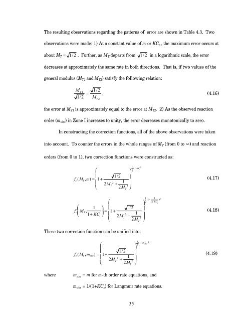
The resulting observations regarding the patterns of error are shown in Table 4.3. Two observations were made: 1) At a constant value of m or KC s , the maximum error occurs at about M T = 1/2 . Further, as M T departs from 1/2 in a logarithmic scale, the error decreases at approximately the same rate in both directions. That is, if two values of the general modulus (M T1 and M T2) satisfy the following relation: M T 1 1/2 = 1/2 M T2 , (4.16) the error at M T1 is approximately equal to the error at M T2. 2) As the observed reaction order (m obs) in Zone I increases to unity, the error decreases monotonically to zero. In constructing the correction functions, all of the above observations were taken into account. To counter the errors in the whole ranges of M T (from 0 to ∞) and reaction orders (from 0 to 1), two correction functions were constructed as: ⎛ ⎜ fc (MT ,m) = 1 + ⎜ ⎝ 1/2 2 1 2MT + 2 2MT ⎛ 1 fc MT , ⎝ 1+ KCs ⎜ ⎛ ⎞ ⎜ ⎟ = 1 + ⎠ ⎜ ⎝ ⎞ ⎟ ⎟ ⎠ 1/2 1 (1−m )2 2 2 1 2MT + 2 2MT These two correction function can be unified into: ⎛ ⎜ fc (MT ,mobs) = 1+ ⎜ ⎝ 1/2 2 1 2MT + 2 2MT 35 ⎞ ⎟ ⎟ ⎠ ⎞ ⎟ ⎟ ⎠ 1 2 (1− mobs )2 1 2 (1− 1 ) 1+ KCs 2 where m obs = m for m-th order rate equations, and m obs = 1/(1+KC s) for Langmuir rate equations. (4.17) (4.18) (4.19)
- Page 3 and 4: BRIGHAM YOUNG UNIVERSITY As chair o
- Page 5 and 6: CBK model uses: 1) an intrinsic Lan
- Page 7 and 8: Table of Contents List of Figures..
- Page 9: Appendices.........................
- Page 12 and 13: Figure A.2. Mass releases of the Ko
- Page 14 and 15: Table 7.6. Parameters Used in Model
- Page 16 and 17: Ed activation energy of desorption,
- Page 18 and 19: vc the volume of combustible materi
- Page 21 and 22: Background 1. Introduction The rate
- Page 23: the CBK model developed at Brown Un
- Page 26 and 27: Zone III rate ∝ C og E obs → 0
- Page 28 and 29: coal-general kinetic rate constants
- Page 30 and 31: Boundary Layer Diffusion The molar
- Page 32 and 33: = q obs q max The factor can be use
- Page 34 and 35: where k 1 and K are two kinetic par
- Page 36 and 37: particle can therefore be convenien
- Page 38 and 39: This is the first time that the gen
- Page 40 and 41: Data of Mathias Mathias (1996) perf
- Page 42 and 43: urn with shrinking diameters, and t
- Page 45 and 46: 3. Objectives and Approach The obje
- Page 47 and 48: Introduction 4. Analytical Solution
- Page 49 and 50: Task and Methodology Task One of th
- Page 51 and 52: 2 [ (i +1) − (i − 1)] i b = −
- Page 53: Table 4.1. The Relative Error * (%)
- Page 57 and 58: correction. The values of functions
- Page 59 and 60: Table 4.6. The Relative Error* (%)
- Page 61 and 62: Table 4.8. The Relative Error* (%)
- Page 63 and 64: general asymptotic solution. An arc
- Page 65 and 66: 5. Theoretical Developments The int
- Page 67 and 68: order of a reaction is usually dete
- Page 69 and 70: nobs = 1 (KCs ) 2 2 1 [KCs − ln(1
- Page 71 and 72: The observed reaction order in Zone
- Page 73 and 74: Bulk Diffusion vs. Knudsen Diffusio
- Page 75 and 76: where D K is in cm 2 /sec, r p is t
- Page 77 and 78: where T p is in K, P is in atm. The
- Page 79 and 80: Both of these assumptions are argua
- Page 81 and 82: 2 r obs ′ − [kD Pog + k d + kD
- Page 83 and 84: oxygen partial pressure (Suuberg et
- Page 85 and 86: Farrauto and Batholomew (1997) prop
- Page 87: assumes a homogeneous, non-interact
- Page 90 and 91: Single-Film Char Oxidation Submodel
- Page 92 and 93: where and An energy balance is used
- Page 94 and 95: where is the empirical burning mode
- Page 96 and 97: calculation uses a 7 × 7 × 7 matr
- Page 98 and 99: HP-CBK Model Development The HP-CBK
- Page 100 and 101: Effective Diffusivity The major obs
- Page 102 and 103: where r p1 and r p2 are the average
The resulting observations regarding the patterns of error are shown in Table 4.3. Two<br />
observations were made: 1) At a constant value of m or KC s , the maximum error occurs at<br />
about M T = 1/2 . Further, as M T departs from 1/2 in a logarithmic scale, the error<br />
decreases at approximately the same rate in both directions. That is, if two values of the<br />
general modulus (M T1 and M T2) satisfy the following relation:<br />
M T 1<br />
1/2<br />
= 1/2<br />
M T2<br />
, (4.16)<br />
the error at M T1 is approximately equal to the error at M T2. 2) As the observed reaction<br />
order (m obs) in Zone I increases to unity, the error decreases monotonically to zero.<br />
In constructing the correction functions, all of the above observations were taken<br />
into account. To counter the errors in the whole ranges of M T (from 0 to ∞) and reaction<br />
orders (from 0 to 1), two correction functions were constructed as:<br />
⎛<br />
⎜<br />
fc (MT ,m) = 1 +<br />
⎜<br />
⎝<br />
1/2<br />
2 1<br />
2MT + 2 2MT ⎛ 1<br />
fc MT ,<br />
⎝ 1+ KCs ⎜<br />
⎛<br />
⎞ ⎜<br />
⎟ = 1 +<br />
⎠ ⎜<br />
⎝<br />
⎞<br />
⎟<br />
⎟<br />
⎠<br />
1/2<br />
1<br />
(1−m )2<br />
2<br />
2 1<br />
2MT + 2 2MT These two correction function can be unified into:<br />
⎛<br />
⎜<br />
fc (MT ,mobs) = 1+<br />
⎜<br />
⎝<br />
1/2<br />
2 1<br />
2MT + 2 2MT 35<br />
⎞<br />
⎟<br />
⎟<br />
⎠<br />
⎞<br />
⎟<br />
⎟<br />
⎠<br />
1<br />
2 (1− mobs )2<br />
1<br />
2 (1−<br />
1<br />
)<br />
1+ KCs 2<br />
where m obs = m for m-th order rate equations, and<br />
m obs = 1/(1+KC s) for Langmuir rate equations.<br />
(4.17)<br />
(4.18)<br />
(4.19)


