NONLINEAR CONTROLLER COMPARISON ON A BENCHMARK ...

NONLINEAR CONTROLLER COMPARISON ON A
BENCHMARK SYSTEM
by
J. Willard Curtis III
A thesis submitted to the faculty of
Brigham Young University
in partial ful llment oftherequirements for the degree of
Master of Science
Department ofElectrical and Computer Engineering
Brigham Young University
April 2000

Copyright c 2000 J. Willard Curtis III
All Rights Reserved

BRIGHAM YOUNG UNIVERSITY
GRADUATE COMMITTEE APPROVAL
of a thesis submitted by
J. Willard Curtis III
This thesis has been read by each member of the following graduate committee and
by majority vote has been found to be satisfactory.
Date Randy W. Beard, Chair
Date Wynn Stirling
Date Timothy McLain

BRIGHAM YOUNG UNIVERSITY
As chair of the candidate's graduate committee, I have read the thesis of J. Willard
Curtis III in its nal form and have found that (1) its format, citations, and bibliographical
style are consistent and acceptable and ful ll university and department
style requirements (2) its illustrative materials including gures, tables, and charts
are in place and (3) the nal manuscript is satisfactory to the graduate committee
and is ready for submission to the university library.
Date Randy W. Beard
Chair, Graduate Committee
Accepted for the Department
Accepted for the College
A. Lee Swindlehurst
Graduate Coordinator
Douglas M. Chabries
Dean, College of Engineering and Technology

ABSTRACT
NONLINEAR CONTROLLER COMPARISON ON A BENCHMARK SYSTEM
J. Willard Curtis III
Department ofElectrical and Computer Engineering
Master of Science
The quest for practical, robust, and e ective nonlinear feedback controllers
has been an area of active research in recent years. One of the challenges in this
research ishowtoevaluate the performance of new nonlinear control strategies, given
that the set of nonlinear systems is so varied. A benchmark problem for nonlinear
systems has been proposed, in order to provide a standard testbed for newly devel-
oped, nonlinear control algorithms. This benchmark problem is an ideal system on
which to apply the Successive Galerkin Approximation to the optimal nonlinear full-
state feedback problem. The Successive Galerkin Approximation (SGA) technique
provides an approximation to the solution of the Hamilton-Jacobi equations associ-
ated with optimal nonlinear control theory. The main contribution of this thesis is
the comparison of the SGA algorithm to four other control methodologies, each of
which is implemented on a hardware system that can be modeled as the nonlinear
benchmark problem. The results show that the SGA algorithms provide excellent
performance and good robustness properties when applied to this benchmark system,
outperforming a simple passivity-based control, two standard linearized controls, and
a simpli ed backstepping control.

ACKNOWLEDGMENTS
I would like to acknowledge my advisor Dr. Beard for all of his assistance
and guidance in the direction of the research that culminated in the thesis. He has
been a wonderful mentor, always willing to help me understand the intricacies of the
mathematics and the subtleties of the eld of robust control. He has always been
supportive of my ideas and a useful source of knowledge and experience.
I would also like toacknowledge the encouragement I received from my other
committee members Dr. Mclain and Dr. Stirling, and for their support of my en-
deavors.
I thank my family and friends wholeheartedly: I'm lucky to have a kind and
patient family, and I'm indebted to them for their love and support, and for their
quiet encouragement of my studies. Thanks to my friends also, for your fellowship.
Especially, I'd like to thank Miguel Apeztegia for his friendship and support, and his
aide in preparing this thesis.

Contents
Acknowledgments vi
List of Tables ix
List of Figures xii
1 Introduction 1
1.1 Motivation and Problem Description . . . . . . . . . . . . . . . . . . 1
1.2 Contributions . . . . . . . . . . . . . . . . . . . . . . . . . . . . . . . 3
1.3 Literature Review . . . . . . . . . . . . . . . . . . . . . . . . . . . . . 4
2 Plant Speci cations and Model 7
2.1 Hardware Set-up and Speci cations . . . . . . . . . . . . . . . . . . . 7
2.2 Derivation of the Mathematical Model . . . . . . . . . . . . . . . . . 8
2.3 Software Set-up . . . . . . . . . . . . . . . . . . . . . . . . . . . . . . 13
3 Overview of Control Strategies Implemented on the Flexible Beam
System 15
3.1 Linear Quadratic Regulation . . . . . . . . . . . . . . . . . . . . . . . 15
3.2 Linear H1 Control . . . . . . . . . . . . . . . . . . . . . . . . . . . . 17
3.3 Passivity-Based Control . . . . . . . . . . . . . . . . . . . . . . . . . 19
3.4 Backstepping . . . . . . . . . . . . . . . . . . . . . . . . . . . . . . . 21
3.5 Successive Galerkin Approximations . . . . . . . . . . . . . . . . . . . 24
3.5.1 The H 2 Problem . . . . . . . . . . . . . . . . . . . . . . . . . 24
3.5.2 The H1 Problem . . . . . . . . . . . . . . . . . . . . . . . . . 27
vii

4 Simulation Results 29
4.1 The Simulated Testbed . . . . . . . . . . . . . . . . . . . . . . . . . . 29
4.2 Evaluation of the Plots in Simulation . . . . . . . . . . . . . . . . . . 31
4.2.1 Linearized Optimal H 2 . . . . . . . . . . . . . . . . . . . . . . 31
4.2.2 Linearized H1 . . . . . . . . . . . . . . . . . . . . . . . . . . 33
4.2.3 Passivity Based Control . . . . . . . . . . . . . . . . . . . . . 33
4.2.4 Backstepping Algorithm . . . . . . . . . . . . . . . . . . . . . 34
4.2.5 SGA: Nonlinear H 2 Optimal Control . . . . . . . . . . . . . . 36
4.2.6 SGA: Nonlinear H1 Control . . . . . . . . . . . . . . . . . . . 39
4.3 Tabulated Results . . . . . . . . . . . . . . . . . . . . . . . . . . . . . 45
4.4 Tuning and Ease of Implementation . . . . . . . . . . . . . . . . . . . 45
4.5 Robustness Analysis . . . . . . . . . . . . . . . . . . . . . . . . . . . 46
5 Experimental Results 49
5.1 Testbed and Open Loop Response . . . . . . . . . . . . . . . . . . . . 49
5.2 Linearized Optimal and Robust Controls . . . . . . . . . . . . . . . . 49
5.3 Passivity Based Control . . . . . . . . . . . . . . . . . . . . . . . . . 50
5.4 Successive Galerkin Approximations . . . . . . . . . . . . . . . . . . . 52
5.5 Tabulated Results . . . . . . . . . . . . . . . . . . . . . . . . . . . . . 59
6 Conclusion and Future Work 61
6.1 Overview . . . . . . . . . . . . . . . . . . . . . . . . . . . . . . . . . . 61
6.2 Extensions to this Research . . . . . . . . . . . . . . . . . . . . . . . 62
Bibliography 66

List of Tables
4.1 Tabular Comparison of Simulated Results . . . . . . . . . . . . . . . 45
4.2 Tabular Comparison of Simulated Robustness . . . . . . . . . . . . . 47
5.1 Tabular Comparison of Experimental Results . . . . . . . . . . . . . . 59
ix

List of Figures
1.1 TORA System . . . . . . . . . . . . . . . . . . . . . . . . . . . . . . 2
2.1 Photograph of Flexible Beam System . . . . . . . . . . . . . . . . . . 8
2.2 Mechanical Model of Flexible Beam System, . . . . . . . . . . . . . . 9
2.3 Torsional Spring Model of FBS . . . . . . . . . . . . . . . . . . . . . 10
2.4 Translational Oscillation Model for FBS . . . . . . . . . . . . . . . . 11
2.5 Simulink Diagram of FBS . . . . . . . . . . . . . . . . . . . . . . . . 14
4.1 Initial Open Loop Disturbance . . . . . . . . . . . . . . . . . . . . . . 30
4.2 Initial Open Loop Response . . . . . . . . . . . . . . . . . . . . . . . 30
4.3 Linearized Optimal vs. Open Loop Response . . . . . . . . . . . . . . 32
4.4 Linear H1 vs. Open Loop Response . . . . . . . . . . . . . . . . . . 33
4.5 Linear H1 vs. Linearized Optimal . . . . . . . . . . . . . . . . . . . 34
4.6 Passivity Based Control vs. Open Loop Response . . . . . . . . . . . 35
4.7 Passivity Based Control vs. Linear Optimal Control . . . . . . . . . . 35
4.8 Passivity Based Control vs. Linear Robust Control . . . . . . . . . . 36
4.9 Backstepping vs. Open Loop Response . . . . . . . . . . . . . . . . . 37
4.10 Backstepping vs. Linear Optimal Control . . . . . . . . . . . . . . . . 37
4.11 Backstepping vs. Linear Robust Control . . . . . . . . . . . . . . . . 38
4.12 Backstepping vs. Passivity Based Control . . . . . . . . . . . . . . . 38
4.13 SGA: Nonlinear H 2 vs. Open Loop Response . . . . . . . . . . . . . . 39
4.14 SGA: Nonlinear H 2 vs. Linear Optimal control . . . . . . . . . . . . . 40
4.15 SGA: Nonlinear H 2 vs. Linear Robust Control . . . . . . . . . . . . . 40
4.16 SGA: Nonlinear H 2 vs. Passivity Based Control . . . . . . . . . . . . 41
4.17 SGA: Nonlinear H 2 vs. Backstepping Control . . . . . . . . . . . . . 41
4.18 SGA: Nonlinear H1 vs. Open Loop Response . . . . . . . . . . . . . 42
xi

4.19 SGA: Nonlinear H1 vs. Linear Optimal Control . . . . . . . . . . . . 42
4.20 SGA: Nonlinear H1 vs. Linear Robust Control . . . . . . . . . . . . 43
4.21 SGA: Nonlinear H1 vs. Passivity Based Control . . . . . . . . . . . . 43
4.22 SGA: Nonlinear H1 vs. Backstepping Control . . . . . . . . . . . . . 44
4.23 SGA: Nonlinear H1 vs. SGA: Nonlinear H 2 . . . . . . . . . . . . . . 44
5.1 Open Loop Response of the FBS . . . . . . . . . . . . . . . . . . . . 50
5.2 Linear Optimal vs. Open Loop . . . . . . . . . . . . . . . . . . . . . 51
5.3 Linear Robust vs. Open Loop . . . . . . . . . . . . . . . . . . . . . . 51
5.4 Linear Robust vs. Linear Optimal . . . . . . . . . . . . . . . . . . . . 52
5.5 Passivity Based vs. Open Loop . . . . . . . . . . . . . . . . . . . . . 53
5.6 Passivity Based vs. Linear Optimal . . . . . . . . . . . . . . . . . . . 53
5.7 Passivity Based vs. Linear Robust . . . . . . . . . . . . . . . . . . . . 54
5.8 SGA: Nonlinear H 2 vs. Open Loop . . . . . . . . . . . . . . . . . . . 54
5.9 SGA: Nonlinear H 2 vs. Linear Optimal . . . . . . . . . . . . . . . . . 55
5.10 SGA: Nonlinear H 2 vs. Linear Robust . . . . . . . . . . . . . . . . . 55
5.11 SGA: Nonlinear H 2 vs. Passivity Based . . . . . . . . . . . . . . . . . 56
5.12 SGA: Nonlinear H1 vs. Open Loop . . . . . . . . . . . . . . . . . . . 56
5.13 SGA: Nonlinear H1 vs. Linear Optimal . . . . . . . . . . . . . . . . 57
5.14 SGA: Nonlinear H1 vs. Linear Robust . . . . . . . . . . . . . . . . . 57
5.15 SGA: Nonlinear H1 vs. Passivity Based . . . . . . . . . . . . . . . . 58
5.16 SGA: Nonlinear H1 vs. SGA: Nonlinear H 2 . . . . . . . . . . . . . . 58
xii

Chapter 1
Introduction
1.1 Motivation and Problem Description
The reliability and e ectiveness of feedback control systems has been recog-
nized for centuries: they provide a simple and robust way of regulating a large class
of physical systems, and there exists a rich body of mathematical results that enable
the systematic design of feedback control laws. A signi cant limitation of most of the
classic results is that they apply to a rather narrow class of systems { those which can
be modeled by systems of linear di erential equations. Despite the fact that many
physical plants can be linearized, and thus an adequate small-signal control can be
realized for the linearized system, the fact remains that almost all physical systems in-
volve dynamics that cannot be modeled completely by a linear system. Such nonlinear
systems have been the subject of much research in the past two decades researchers
have sought to extend the results obtained for linear plants to non-linear plants.
A good example of this is the search for the nonlinear optimal feedback con-
troller. It is well known that the solution of the optimal linear control problem
depends upon the solution of an algebraic Riccati equation. For the non-linear case,
this result generalizes nicely: the optimal non-linear controller requires the solution of
the Hamilton-Jacobi-Bellman (HJB) equation (which was actually discovered before
the Riccati equations). This partial di erential equation is very di cult to solve,
however, and the quest for a reliable and accurate approximation of its solution is an
open problem. The Successive Galerkin Approximation (SGA) is one such method of
approximation, and the details of its implementation will be described in Chapter 3.
1

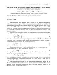
Figure 1.1: TORA System
One of the challenges of evaluating the non-linear control design techniques
that are being developed is to nd a reasonable method of gauging their performance.
There exists a large variation in the complexity, behavior, and dynamics within the
set of non-linear systems, and a given control design might work very well on one
speci c type of system while providing poor performance on another. Thus the need
for a benchmark non-linear problem { a mathematical system that contains signi cant
non-linearities, has a tractable mathematical model, and is fairly easy to implement
in hardware.
In recent years, the translational oscillator rotational actuator (TORA) [1]
system (also referred to as the Non-linear Benchmark Problem or NLBP) has been
proposed as just such a benchmark system. In this system a mass is restricted to a
linear oscillatory motion by ideal springs, and the system is actuated by arotational
proof mass. The coupling between the rotational and linear motion provides the non-
linearity. Many di erent researchers have used this system as a testbed to evaluate
various non-linear control strategies, so this system was selected as a way to eval-
uate and compare the performance of the successive Galerkin technique with other
robust, non-linear control laws as well as with standard optimal linearized methods.
Speci cally, six unique control laws are derived and implemented on a hardware im-
plementation of the TORA system. A non-linear Galerkin approximation to the H 2
2

problem and a Galerkin approximation to the non-linear H1 problem are studied and
compared with the results of a linearized optimal control, a linearized H1 control, a
passivity-based control, and a control law based on integrator backstepping. These
control strategies are chosen because they are current topics of research, and most
are proposed as control laws that will be provide robust performance.
The speci c hardware system, upon which the tests were performed, is de-
scribed in Chapter 2 along with a derivation of the equations of motion. Chapter 3
presents an overview of the control strategies tested, and it explains the details of the
implementations of each algorithm. Chapter 3 also explains the successive Galerkin
approximation technique and shows how it is implemented on the hardware system.
Chapter 4 explains the mechanics of the testbed and the methods of comparing per-
formance, and a comparison of the six controls in simulation is presented. The actual
results of the tests as performed in hardware are compared and discussed in Chap-
ter 5, and an analysis of the robustness of the control laws is presented in Chapter
6. Finally Chapter 7 sums up the results of the experiment the conclusions of the
research are presented along with recommendations for future research.
1.2 Contributions
There is often a wide gap between mathematical systems and the physical
plants these systems attempt to model. The TORA system is proposed in [2] as
a benchmark problem so that nonlinear control algorithms can be compared on a
common system { a system that can be easily implemented in hardware. While many
control designs perform well in the idealized environment of mathematics, the true
test of a nonlinear algorithm must lie in its regulation of a physical plant. The SGA
technique is applied to the nonlinear benchmark problem, and it performs better than
other well known nonlinear techniques when applied to a physical implementation of
this TORA system. This result is the main contribution of this thesis: it o ers
experimental evidence that the SGA method produces excellent results when applied
to real-life problems and systems. This thesis also justi es further research into
understanding, clarifying, and improving the SGA technique.
3

1.3 Literature Review
In surveying the technical literature relevant to this thesis, there are two pri-
mary topics: research on the topic of the successive Galerkin approximation method,
and research devoted to the topic of the NLBP system. Additionally a short review of
the literature pertaining to the various control strategies used to highlight the SGA
method will be presented.
The SGA method was rst published in [3] as a method for iteratively improv-
ing a nonlinear feedback control. This publication included a proof of the algorithm's
convergence and the stability of the resulting control law at each iteration. Addi-
tionally, each iteration brings the control design closer to solving the HJB equation,
and thus the method of successive approximation eventually yields an approxima-
tion of the nonlinear optimal solution with any desired accuracy, as the order of the
Galerkin approximation increases and as the number of iterations goes to in nity.
In [4] the algorithm was successfully applied to the inverted pendulum problem as
well as several one-dimensional examples. In [5] the SGA technique was extended to
the optimal robust nonlinear control problem. In the robust problem, a solution of the
Hamilton-Jacobi-Isaacs equation is required with the minimum possible L 2 gain from
disturbance to output. In [5] a proof is presented of the convergence and stability of
the algorithm at each successive iteration, and su cient conditions for convergence
and stability are presented for both the nonlinear optimal and robust algorithms.
Additionally, [5] successfully applies the algorithm to a hydraulic actuation system,
a missile autopilot design, and the control of an underwater vehicle system.
The control of the TORA system was originally proposed as a model of a
dual-spin spacecraft. The goal was to study how to circumvent the resonance capture
e ect in [6], but in [7], [8] the system was studied to analyze the usefulness of a
rotational actuator in damping out linear oscillations and vibrations. It was rst
proposed as a benchmark problem for nonlinear control systems in [2]. A physical
testbed is described consisting of a motor driven proof mass that was mounted on a
linear air track. In [2], the three-fold objective of the Nonlinear Benchmark Problem
is set forth: to stabilize the closed loop system, to exhibit good disturbance rejection
4

compared to the uncontrolled oscillator, and to require limited control e ort. A
passivity-based control design is also described that uses the control to simulate a
damped pendulum absorber. The International Journal of Robust and Nonlinear
Control published a special issue devoted exclusively to the NLBP (volume 8, 1998)
and the 1995 American Control Conference contained an invited session in which six
papers were submitted on the topic of the Nonlinear Benchmark Problem.
The literature devoted to the TORA system was used as the basis for the
designs presented in this thesis. In particular, the passivity-based control strategy
comes mainly from the implementation described in [9], while a more complete ex-
planation of passivity-based control of Euler-Lagrange systems can be found in [10]
or in [11]. The integrator backstepping controller was mainly derived from [1] where
they supply the necessary variable substitutions and transformations to derive acas-
cade controller. It should be noted that the cascade controller presented in [1] is
almost identical to the one derived in this thesis, and this controller is a special case
of the full controller one obtains using integrator backstepping as described in [12].
The linearized optimal H 2 controller was derived by the well known solution to the
Riccati equation. A concise overview of the theory and application of optimal linear
control can be found in [13]. The linearized H1 controller was also designed by the
well known robust control technique as described in Chapter 6 of [14].
5

Chapter 2
Plant Speci cations and Model
2.1 Hardware Set-up and Speci cations
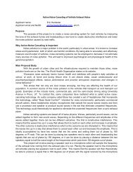
The various control strategies studied in this thesis are implemented on the
same experimental testbed, which consists of a Flexible Beam System (FBS) that
was purchased from Quanser Consulting Inc. A picture of the FBS upon which the
control experiments were conducted is shown in Figure 2.1.
It consists of a thin metal beam that is clamped at one end while free at the
other. The free end is equipped with a voltage controlled DC motor that rotates a
rigid beam structure this structure acts as a proof mass, and it's rotation is the only
actuation mechanism in the system. The object of the control is to actuate this proof
mass in such away that its motion will damp an initial vibration in the exible beam.
The whole system consists of four parts:
1) A exible beam,
2) A proof mass structure consisting of two rigid beams and a cross beam,
3) A DC motor and an encoder,
4) A base plate instrumented with a strain gauge.
The exible beam is 44 cm in length, while the rigid beams that form the proof
mass are 28.5 cm in length. The rst mode sti ness of the system is experimentally
derived by measuring the natural frequency, anditsvalue is approximately 30 N . The
m
mass of the cross bar that acted as the proof mass is .05 kg, with the inertia of the
rigid beams connecting the cross bar to the motor is found to be :0039Kgm 2 . The DC
motor has an external gear ratio of 70 to 1, an electrical resistance of 2.6 ohms, and a
7

Figure 2.1: Photograph of Flexible Beam System
torque constant of .001 Nm/Amp. The motor served as the only input to the system,
however a strain gauge placed near the xed end of the exible beam senses the
beam's de ection, and an encoder on the motor senses the angular position the proof
mass. The strain gauge is calibrated to give 1 Volt per inch, and the encoder uses a
1024 count disc which in quadrature results in a resolution of 4096 counts/revolution.
The FBS can be mounted in two con gurations, with the exible beam vertically or
horizontally mounted. We choose to mount the beam horizontally so that gravity will
be acting perpendicular to the motion of the system, thus making stabilization more
di cult.
2.2 Derivation of the Mathematical Model
Obtaining an adequate mathematical model for the FBS, one that was not too
complex to be useful nor one that was too simple to be accurate, is a challenge. The
rst step is representing the physical system in a simpler way. Figure 2.2 shows a
simple mechanical model of the system. Here the rigid beam structure is modeled as a
single rigid beam with a point mass (m) located at one end and a motor at the other.
8

Figure 2.2: Mechanical Model of Flexible Beam System,
The exible beam is treated as capable only of motion in the plane of the diagram.
If perturbed the free end of the beam will oscillate according to the classical beam
equation:
A(x) @2 w(x t)
@t 2
+ @2
@x 2 [EI(x)@2 w(x t)
@x 2 ]=f(x t) (2.1)
where f(x t) is the applied force on the beam in the y direction,and w(x t) is the
de ection of a point a distance x from the xed end at time = t. Unfortunately, the
partial derivatives in this equation are not suitable for the state-space model that we
seek, something of the form:
where x 2 IR n .
_x = f(x)+g(x)u(x) (2.2)
A simpler idea would be to model the exible beam as a rigid beam with a
single torsional spring at the xed end (see Figure 2.3). A state-space equation can
be obtained for this model using the Euler-Lagrange (EL) equations:
d
dt (@Lp(qp qp) _
) ;
@qp _
@Lp(qp qp) _
= Mup
@qp
9
(2.3)

Figure 2.3: Torsional Spring Model of FBS
Here, Lp is the Lagrangian (the kinetic energy minus the potential energy) and Mup
is avector representing the external forces applied to the system.
Using these equations, we obtain a model that is unwieldy and di cult to use
in designing control laws, therefore an even simpler model is desired. If one assumes
that the free end of the exible beam undergoes only small de ections, then it can
be assumed to follow a linear path, and its de ection can be measured as a length
rather than as an angle. We can then model the bending dynamics of the beam as
a simple linear spring with spring constant k. The system can then be thought of
as a rotational actuator that either induces or attenuates translational oscillations.
Figure 2.4 shows a simple diagram of this concept. While this model ignores all of the
higher order modes and dynamics of the beam as well as the nonlinear motion of the
free end, it does yield a su ciently simple mathematical representation. The linear
displacement of the motor xture at the free end of the exible beam is represented
by y, is the angle made by the rigid proof mass, k is the equivalent linear sti ness of
the exible beam structure, m is the mass at the end of the proof mass, M is the total
mass of the motor xture, c is the length of the rigid proof mass, Rm is the motor's
10

Figure 2.4: Translational Oscillation Model for FBS
electrical resistance, and I is the inertia of the proof mass. Letting x =(y _y _ ) T ,
and using the voltage applied to the motor as the input to the system, the resulting
state space equations are as follows:
0 1 0
_y
B C B
B C B
ByC
B
B C
B _C
= B
C B
@ A @
_y
_2 Rm sin( )(m 2 c 3 +Imc)+mc cos( ) _ K 2 m K 2 g;ykRm(mc 2 +I)
Rm[(I+mc 2 )(M +m);m 2 c 2 cos 2 ( )]
_
;m2c2Rm cos( )sin( ) _2 +yRmkmc cos( );y(m+M )Rmk
Rm[(I+mc2 )(M +m);m2c2 cos2 ( )]
0
B
+ B
@
1
C
A
0
;mcKmKg cos( )
Rm[(I+mc2 )(M +m);m2c2 cos2 ( )]
0
KmKg(m+M )
Rm[(I+mc 2 )(M +m);m 2 c 2 cos 2 ( )]
1
C u(x) (2.4)
C
A
Again, this state-space model was derived using the EL equations. One mightwonder
at the validity of the simplifying assumptions necessary to derive this model. For the
purpose of this thesis, modeling inaccuracy is highly desirable { the control strategies
studied in this paper are purportedly \robust" in some sense. One would hope that
11

a robust design strategy would, in practice, stabilize a physical plant that di ers
substantially from its mathematical model. Thus the crudeness of our model only
helps to demonstrate the robustness of the control laws that succeed in yielding
adequate performance on the actual hardware system. Another advantage of this
mechanical model is that it is identical, in form, to the system equations presented
in [2] as a nonlinear benchmark problem. Since the object of this research is to
compare nonlinear robust control strategies, this model is ideal in the sense that it
is already widely used as a standard mathematical system for testing and comparing
nonlinear control techniques. The mathematical model in (2.4) is slightly di erent
than the standard model of the NLBP in that our input is voltage, not torque. This
adds one extra term and a few constants in order to incorporate the voltage to torque
transfer function into the model. Many of the papers involving the NLBP express the
system equation in a non-dimensionalized form. Since some of the control strategies in
this comparison make use of these dimensionless equations, and because they simplify
the model by combining all of the physical parameters into a single value, we include
them here:
0 1
_z
B C
B C
BzC
B C
B _ C
@ A
=
Where _ represents d
z = y
= t
=
d q
M +m
I+mc
q
k
M +m
0
B
@
v(x) =u(x) m+M
k(I+mc2 )
mc = p
(I+mc2 )(m+M )
_z
;z+ _2 sin( ); 2 cos( )_z K2 m K2 g
Rmmc
1; 2 cos( ) 2
_
cos( )[z; 2 sin( )]+ K2 m K2 g
Rmmc
1; 2 cos( ) 2
1
C
A
+
0
B
@
0
KmKg
Rm
cos( )
1; 2 cos( ) 2
0
KmKg
Rm
1; 2 cos( ) 2
and the following transformations are used:
12
1
C v(x): (2.5)
C
A

2.3 Software Set-up
All of the control strategies presented in this paper were simulated in MAT-
LAB's SIMULINK environment. They were then implemented by way of Quanser
Consulting's Multiq3 I/O board which interfaced with the SIMULINK Real Time
Workshop. Figure 2.5 shows the SIMULINK model used in the simulations and in
the actual exible beam system. Their are two main blocks, one is the control block
that takes the four states as inputs, as well as an initial open loop disturbance. The
control has only one output, a voltage signal that is fed into the system block. The
output of the strain gauge and the motor encoder were run through the Multiq3
board into SIMULINK. These provided a direct state measurement of the angle, ,
and the strain was a good estimator for the linear displacement, y. The state ve-
locities in the system equations were numerically computed using lters of the form
s
s+
. Although this theoretically makes for a relatively crude observer, in practice
these pseudo derivatives actually performed very well. Even though the assumption
of full-state feedback is not strictly true, in practice a more complicated observer
is unnecessary to achieve good performance by the control laws. The sample rate
for in the SIMULINK model for both the simulation and the FBS was 1 kHz. All
of the physical parameters for the Quanser system are noted here: k = 30N=m,
m = :05Kg, M = :6Kg, c = :285m, I = :0030Kgm 2 , Km = :001Nm=A, Kg = 70,
Rm =2:6 Ohms.
13

printed 09−Mar−2000 09:04
page 1/1
/tmp_mnt/auto/ee/willy/work/simbeam/lqr2a.mdl
Integrate x1^3
Display1
Control
Sequence
In2 Out1
select OL/CL
In1
0
Open loop
2*pi*fnat*2
s+2*pi*fnat*2
2
Limit
thetadot
Filter
Disturbance
U
Disturbance
Sequence
defdot
theta
Figure 2.5: Simulink Diagram of FBS
14
def
Integrate x1^2
Display
LQR Controller
In2 Out1
In1
0
Smart System /curtis
rad −−> deg
theta
theta
−K−
thetadot
Volts
lqr.mat
defdot
input
m −−> cm
position
To File1
def
100
lqr2a

Chapter 3
Overview of Control Strategies Implemented on the Flexible
Beam System
This Chapter will provide a review of all of the control strategies that were
tested on the NLBP. The focus of this thesis is the comparison of the SGA method
of control with a broad sample of current robust nonlinear control methodologies.
Thus the following nonlinear design methodologies are included mainly to highlight
the uniqueness of the SGA design method. This chapter will explain the mathemat-
ical derivation of two linearized controls, a passivity based approach, abackstepping
controller, and the SGA algorithm. Additionally, the details of the implementation
of these controllers will be explained.
3.1 Linear Quadratic Regulation
As a starting point of comparison, an H 2 optimal control was rst designed
for the linearized system. With optimal control, the objective is to minimize a cost
functional of the following form:
V (x 0)=
Z 1
(x
0
T (t)Qx(t)+u T Ru)dt (3.1)
where V (x 0) represents the cost associated with moving from a given state, x 0, under
a control signal u to the origin. Q and R are matrices that weight the cost of the
states and the control respectively. The goal is to nd the stabilizing control signal
u (x) that will minimize the cost V (x). Linear quadratic regulation has a well known
solution, where the optimal stabilizing control u (x) is a simple linear combination of
the states: u (x) =;Kx. K is a matrix that depends upon the input matrix B, the
15

weighting matrix R, and P : K = R ;1 B T P , where P is the solution to the following
algebraic Riccati equation:
0=A T P + PA+ Q ; PBR ;1 B T P (3.2)
As the name implies, a linearization of the system equations is necessary to implement
this control strategy. The linearized equations for system (2.4) were derived as follows:
_~x = rF (x)jx0 ~x + rG(x)jx0 ~u = A~x + B~u (3.3)
where F (x) and G(x) are as de ned in (2.4). A and B are calculated to be:
0
0
B (mc
B
A = B
@
1 0 0
2 +I)k
Mmc2 +I(m+M ) 0 0
mcK2 mK2 g
Rm(Mmc2 1 0
0 0 0
0
C B
C B ;mcKmKg
C B
+I(m+M )) C B = B Rm(Mmc
B
1 C B
A @
0 0
2 1
C
+I(m+M )) C
0 C
A
mck
Mmc 2 +I(m+M )
;K2 mK2 g (m+M )
Rm(Mmc2 +I(m+M ))
(m+M )KmKg
Rm(Mmc 2 +I(m+M ))
(3.4)
After the constants are substituted, the linearized model becomes:
0
1 0 1
0
B
B;48
_x = B 0
@
1
0
0
0
0
0
0
:44
1
0
C B C
C B C
C B;:69C
C x + B C
B C u(x):
C B 0 C
A @ A
(3.5)
86 0 0 ;19:9 31:7
Next, simulations were run to determine which matrices Q and R would result in a
strongly damping control while not running the actuator past it's physical limitations.
Once suitable weighting matrices were obtained, the control was implemented on the
hardware, and the weights were tuned again to give good performance on the physical
plant. Tuning is always a subjective endeavor, and there is no guarantee that the
values we found were, in fact, the absolute best choices, nevertheless the parameters
that we found to give the best performance were the following:
0
1
2000
B 0
Q = B 0
@
0
100
0
0
0
70
0
C
0 C
0C
A
0 0 0 0
R = :01:
16

The optimal gain matrix was given by K =(;658 69:8 26 3:7). Although the LQR
design is simple to derive and easy to implement, it is subject to several weaknesses.
First and foremost, this control strategy is optimized for a mathematical system
quite di erent from the actual hardware. Note that the original model itself is a
large simpli cation of the physical plant, and now even this model has been further
distorted through the linearization process. Hence, the errors in modeling should be
compounded, whereas all of the unmodelled and non-linear dynamics will be ignored
by the LQR design. Another possible limitation of LQR control design is the sim-
plicity of its mechanism: the control signal is limited to be just a linear combination
of the states. Other controls studied in this paper will implement feedback controls
generated by more sophisticated functions of the plant's outputs.
3.2 Linear H1 Control
The objective of a linear H1 controller is to nd a feedback gain u = ;Kx such
that the L 2 gain from an exogenous disturbance signal, w(x), to an output signal,
z(x), is minimized i.e. we must nd a stabilizing u(x) that achieves the smallest
possible gain, :
Z T
0
z(t) T z(t)dt = 2
Z T
0
w(t) T w(t)dt (3.6)
This approach attempts to nd a robust control that will yield adequate performance
even with a worst case disturbance signal, and it is hoped that such a control will then
be robust with respect to the various modeling errors and unmodelled dynamics of
the physical system studied. For our system, the disturbance signal w(x) ismodeled
as the apparent linear force acting on the free end of the exible beam:
0
0
B
KmKg(M +m)
B
_x = f(x)+g(x)u(x)+ B Rm[(I+mc
B
@
2 )(M +m);m2c2 cos2 1
C ( )] C w(x):
0
C
A
(3.7)
;mcKmKg cos( )KmKg
Rm[(I+mc 2 )(M +m);m 2 c 2 cos 2 ( )]
and the output signal z(x) is de ned as a quadratic weighting of the states plus the
control energy. These de nitions are reasonable since the unmodelled and truncated
17

higher order dynamics of the beam should manifest themselves as forces acting on
the beam, while the desired output is the regulation of the states subject to limited
actuator power. Thus the linearized H1 control should, even under worst-case e ects
from modeling and linearization errors, generate an adequate, stabilizing control. Like
the LQR design strategy, linearH1 is a solved problem, the solution of which can be
obtained by solving the following modi ed algebraic Riccati equation:
0=PA+ A T P ; P (B 2B T
2 ; ;2 B 1B T
1 )P + C T C: (3.8)
The valid solutions are ones in which P 0 and are suchthatA;(B 2B 0 2; 2 B 1B 0 1)P is
asymptotically stable. Asearch is then performed to nd the smallest possible that
satis es these conditions, and the resulting solution (a function of this optimal ) is
guaranteed to minimize the L 2 gain from disturbance to output while simultaneously
stabilizing the system. The optimal feedback gain matrix K is next computed from
this solution as follows: K = ;B 0 2P . In these equations, B 1 is the matrix resulting
from a linearization of k(x), where
0
B
k(x) = B
@
0
KmKg(M +m)
Rm[(I+mc2 )(M +m);m2c2 cos2 ( )]
0
;mcKmKg cos( )KmKg
Rm[(I+mc 2 )(M +m);m 2 c 2 cos 2 ( )]
1
C (3.9)
C
A
and B 2 is the linearization of g(x) about the equilibrium point x =0. For the exible
beam system, B2 was found to be:
0 1
0
B C
B C
B;:69C
B2 = B C
B C : (3.10)
B 0 C
@ A
31:7
The parameters used to compute this control were Q = 2000 100 70 0 and
R = :01. The optimal gain matrix was computed to be K = ;62 17 1:5 :46
and the optimal gamma was was found to be = 302.
18

3.3 Passivity-Based Control
Certain physical systems can be pro tably studied by examining the prop-
erties of their potential energy functions, and by noticing the natural damping and
dissipation present. Passivity-Based Control (PBC) algorithms have yielded simple,
yet robust control laws to a variety of such systems by shaping the energy and dis-
sipation functions. The exible beam system is an example of an under-actuated
Euler-Lagrange system, a system that is completely modeled by the EL equations.
The stability of the equilibrium states of EL systems is solely dependent on their
potential energy functions, and if enough damping is present these equilibria will be
asymptotically stable. Passivity-based control designs seek to exploit these facts to
robustly stabilize complicated nonlinear systems. In particular, the potential energy
function of the closed-loop system is shaped by the controller, and suitable damping
is injected into the system via the control law to achieve the desired stability and
performance objectives. There are several fundamental properties of EL systems that
make this energy-shaping and damping injection practical. First, EL systems are
completely described by their EL parameters: TpVpFpM where the EL equation is
written as follows:
d
dt (@Lp(qp qp) _
) ;
@qp _
@Lp(qp qp) _
@qp
= Mup ; @Fp( qp) _
: (3.11)
@ _
In this equation Lp(qp qp) _ = Tp(qp qp) _ ; Vp(qp qp), _ where Tp is the plant's kinetic
energy, Vp is the plant's potential energy, Fp( qp) _ is the Rayleigh dissipation function
for the plant, and M is a vector of ones and zeros that indicates which of the states
are directly actuated by the plant inputs, up. We can now construct a controller as
another EL system as follows:
d
dt (@Tc(qc qc) _
) ;
@qc _
@Tc(qc qc) _
+
@qc
@Vc(qcqp)
+
@qc
@Fp( qp) _
=0: (3.12)
@qp _
Here, the potential energy function of the control block, Vc, is a function of the plant
states qp and the control state qc, but its not a function of the generalized control
velocity qc. _ This equation can be combined with the EL equation for the plant into
19
qp

a total closed-loop expression, provided that the plant input, up, is de ned according
to the following interconnection constraint:
up = ; @Vc(qcqp)
: (3.13)
@qp
Thus, the second and most important factabout EL systems is that the closed-loop
system is itself an EL system, and the closed-loop EL parameters (TclVclFcl) are
simply the sum of the parameters of the plant and the control. In other words,
we can shape the energy and dissipation of the closed loop system as desired by
choosing the dynamics of the control in the correct manner: it must comply with
the aforementioned interconnection constraint. In [10] this idea is further re ned
by showing that the injected dissipation function in the control need not necessarily
be a function of the derivative of the plant variables. Rather, a dynamic system in
the control is su cient, under certain passivity conditions on the original plant, to
guarantee closed loop asymptotic stability. In addition, Ortega et.al. [10] add the
constraint thatthere is limited actuator power available, or in other words
up umax: (3.14)
Following the design outlined in [15], a suitable Rayleigh dissipation function Fc was
chosen:
Fc = 1
2ab _
qc
(3.15)
where a and b are parameters that scale the injected damping. Also, the potential
energy function of the control was constructed so as to ensure the stability of the zero
equilibrium point. A su cient condition is that Vcl = Vp + Vc have a global minimum
at zero. Since the potential energy of the plant is a quadratic function of the states,
we chose Vc as
Vc(q3qc) = 1
Z Z qc+bq3
q3
k1 tanh(s)ds + k2 tanh(s)ds: (3.16)
b 0
0
so that it was the sum of two strictly increasing integrals that are minimized at the
zero state. Here tanh(s) was chosen as a saturation function to model the actuator
20

limitations, k 1 and k 2 are tuning parameters to properly shape the closed loop en-
ergy function, and q 3 is the actuated plant variable, . The controller dynamics are
computed from the interconnection constraint andthe controller's EL equation:
u = ;k 2 tanh(qc + b ) ; k 1 tanh( )
qc _ = ;ak2 tanh(qc + b ):
(3.17)
Thus the control takes the measurable output, , as its only input, and the dynamics
in the control produce a pseudo-derivative of to generate the necessary damping.
The mathematical model for the exible beam system was slightly di erent from the
nonlinear benchmark problem due to the extra term that resulted from the fact that
we used voltage as an input instead of torque. This made the implementation of the
saturation constraint a little tricky. In fact, the particular software/hardware con g-
uration of the exible beam system required the removal of the saturation functions
in the controller dynamics. (The actual control signal was up = ;k 2(qc + b ) ; k 1 .)
To implement the control was simple: nd appropriate values for a b k 1 and k 2.
The constants a = 250, b = 2:7, k 1 = :29 and k 2 = 2:5 were chosen experimentally
to give the best possible dynamic performance. This control was relatively easy to
implement, and its great advantage is that it only uses measurable outputs of the
system. This strength can also be seen as a weakness, though the controller does
not utilize all of the available information { only one of the two truly measurable
states is used to generate the control signal. From an informational stand-point, the
ideal controller should use all of the available plant output signals. However, the
passivity-based control can clearly do more than a feedback system consisting of a
simple gain matrix { PBC systems implement a dynamic system in the feedback loop
that, in our case, provides information about _ as well as .
3.4 Backstepping
Another recent approach to the problem of robustly stabilizing non-linear sys-
tems is that of integrator backstepping. This control strategy is an attempt to con-
struct for a given non-linear system a control that will render the closed-loop system's
21

control Lyapunov function globally asymptotically stable. Backstepping essentially
tries to reduce the system to a number of subsystems in series. Then the stabilizing
inputs for the subsystem closest to the output are computed, and these inputs are
then treated as the outputs of the previous system, and a new set of inputs to this
next subsystem are computed to guarantee stability. This process is repeated until
the original control input is computed. Control laws generated by this methodol-
ogy, as shown in [1], are proven to stabilize the system globally and asymptotically.
However, this design procedure is the most di cult to compute and implement, and
the resulting control law is both complicated and cumbersome. The rst step is
to apply a variable transformation to the exible beam's non-dimensionalized state
equations (2.5) to obtain:
z 1 = x 1 + sin( )
z 2 = x 2 + _ cos( )
y 1 = x 3
y 2 = x 4
v =
1
1 ; 2 cos 2 ( )
cos( )(z1 ; (1 + _2 ) sin( )) + k2 mk2 g
Rmmc (z2 ; _ cos( )) + kmkgu
R ; m
(3.18)
This variable substitution and the feedback transformation from u to v (which is
a non-singular transformation because the parameter is always smaller than 1)
simpli ed the system equations to the following form:
z_ 1 = z2 z_ 2 = ;z1 + sin( )
y_ 3 = _
y_ 4 = = v
22
(3.19)

Now we regard as the control variable and construct a control law y 1( ) that
will make the translational coordinates (z 1 and z 2) globally asymptotically stable.
Jankovic et.al. [1] choose y 1( )=; arctan(c 0z 2). However, y 1 is not the control vari-
able, and it follows its own dynamic equations. Therefore we de ne new angular
variables to implement the desired trajectories of and _ : 1 = + arctan(c 0z 2) and
2 = _ 1. Substituting into the previous system equation yields the following modi ed
system equation:
z_ 1 = z2 z_ 2 = ;z1 + sin( 1 ; arctan(c0z2)) _ 1 = 2
_ 2 = w
w = v ; 2c3 0z2 1+c2 0z2 (;z1 + sin( ))
2
2 +
c 0
1+c 2
0z2 2
(;z 2 + _ cos( )):
(3.20)
Now all that is required is to stabilize the -subsystem which can be done with the
simple feedback w = ;K . By following the approach outlined in [1], but with the
system modi ed for voltage as the input instead of torque, the following control law
is obtained:
u = k(I + mc2 )
m + M
= ;k1(y1 + arctan(c0z2)) ; k _
k2c0(;z1 + sin( )
2 ;
1+c2 0z2 2
+ 2c0z2(;z1 + sin( )) 2
(1 + c2 0z2 2) 2 + c0(;z2 + _ cos( )
1+c2 0z2 2
mc
= p
2 (I + mc )(m + M)
(3.21)
The primary di culty with implementing this control is understanding the purposes
of the various transformations and substitutions. Additionally, this last expression for
the control input is quite complicated { this makes it di cult to assign physical mean-
ing to the control parameters, c 0, k 1, k 2. The parameters used in the commissioning
of this design are as follows: c 0 =1,k 1 = 10, and k 2 =1.
23

3.5 Successive Galerkin Approximations
The primary purpose for implementing the four previous designs was to pro-
vide a reasonably complete set of control laws with which to compare the successive
Galerkin approximation algorithm as developed in [5]. This control strategy seeks to
solve the non-linear H 2 and H1 problems by approximating the solutions to their
associated Hamilton-Jacobi equations. These equations are non-linear partial dif-
ferential equations that are impossible to solve analytically in the general case. To
accomplish the approximation the Hamilton-Jacobi equations are rst reduced to an
in nite sequence of linear partial di erential equations, named generalized Hamilton-
Jacobi equations. Second, Galerkin's method is used to approximate the solutions
of these linear equations, and the combination of these two steps yields a control
algorithm that converges to the optimal solution as the order of the approximation
and the number of iterations goes to in nity.
3.5.1 The H 2 Problem
The SGA technique was rst applied to the non-linear optimal H 2 problem,
where the goal is to minimize a cost functional V with respect to some u (x):
_x = f(x)+g(x)u
Z
V (x) =min l(x)+kuk
u
2
R dt
where l(x) is some cost function that depends on the state x, and R is the matrix
that weights the cost of the control. Throughout this development we shall assume
that f(0) = 0, that l(x) is a positive de nite function, and that f(x) is observable
through l(x). The solution to this minimization problem is given by the full-state
feedback control law
u (x) =; 1
2 R;1 T @V
g
@x
24
(3.22)

where V satis es the well known Hamilton-Jacobi-Bellman (HJB) equation, written
as follows:
@V T
@x
1 @V
f + l ;
4 @x gR;1 T
T @V
g
@x
=0: (3.23)
To implement the rst step of the SGA algorithm we write the HJB equation as
@V T
@x
(f + gu)+l + kuk2 R =0 (3.24)
u (x) =; 1
2 R;1 T @V
g
@x
: (3.25)
Equation (3.24), a linear partial di erential equation, is the Generalized Hamilton-
Jacobi Bellman equation (GHJB). The usefulness of writing the HJB equation in
this form is that now V and u are decoupled. Assuming that we start with some
stabilizing control, u (0) (x), we can perform an in nite sequence of iterations to nd
the optimal control, u (x):
@V (i)T
@x (f + gu(i) )+l(x)+
(i)
u
2
=0 R (3.26)
u (i+1) (x) =; 1
2 R;1g T (i) @V
(x) (x)
@x
(3.27)
where i ranges from 0 to 1. If u (0) (x) asymptotically stabilizes the system on IR n ,
then Equations (3.26) and (3.27) describe a sequence of iterations, which was shown
in [16] to converge to the solution of the HJB equation point wiseon . Thus instead
of computing V and u simultaneously as in the HJB equation, we compute them
iteratively. The only problem left is to solve the GHJB equation at each step of the
iteration.
The solution V (i) of Equation (3.26) on can be approximated via a global
Galerkin approximation scheme as follows. Let V (i)
N (x) = PN j=1 c(i)
j
j(x), where the
set f j(x)g 1 j=1 is a complete basis for L 2( ) and j(0) = 0. The coe cients c (i)
j are
found by solving the algebraic Galerkin equation
Z
@V (i)T
@x (f + gu(i) )+l +
(i)
u
2
R
k =1:::N.
25
k dx =0

To apply this algorithm to the exible beam system, we made use of a Matlab
implementation of this algorithm contained in the le hjb.m (see Appendix B). It is
a straightforward numerical implementation of the preceding algorithm, and it only
required three items: the set , the basis elements f jg N
j=1, and the initial stabiliz-
ing control u (0) . In the hardware implementation we used the following initializing
parameters:
=[;:2:2] [;2:5 2:5] [; 2 2 ] [;20 20]
f jg = fx 2
1x 2
2x 2
3x 2
4x 1x 2x 1x 3x 1x 4x 2x 3x 2x 4x 3x 4g
u (0) (x) =41x 1 ; 1:5x 2 ; 2:6x 3 ; :19x 4:
We added higher order terms in simulation, though they only slightly improved the
performance:
=[;:05:05] [;5 5] [; 2 2 ] [;10 10]
f jg = fx 2
1x 2
2x 2
3x 2
4x 1x 2x 1x 3x 1x 4x 2x 3x 2x 4x 3x 4x 3
1x 2x 1x 3
2x 3
1x 3x 3
2x 3x 1x 3
3
x 2x 3
3x 3
1x 4x 3
2x 4x 3
3x 4x 1x 3
4x 2x 3
4x 3x 3
4g
u (0) (x) = 120x 1 ; 25x 2 ; 4:5x 3 ; :6x 4:
In other words, we made the initial stabilizing control the linearized LQR control
developed previously. was constructed so that the control would be stabilizing for
displacements of up to 20 cm in either direction and for rotations of up to 90 degrees
by the proof mass, in the hardware. The basis functions were simply a set of second
order polynomials and their corresponding cross terms, and in the simulation fourth
order terms were added as basis functions. This control has several bene cial qualities.
First, it uses all of the available outputs to generate a truly non-linear control signal {
u(x) can depend on the square of the states, and the g T (x) term renders even a second
order SGA control signal nonlinear. Second, the SGA algorithm is approximating an
optimal solution: the designer can feel assured that the control approaches optimality
with respect to the desired cost functional. Third, the SGA algorithm is easy to tune
26

ecause one can quickly adjust the Q and R matrices to change the state penalty
weightings. Finally, this design technique can be interpreted as improving upon the
initial stabilizing control (developed through some sub-optimal approach, such as a
backstepping or PBC strategy) at each iteration of the algorithm.
3.5.2 The H1 Problem
The successive Galerkin approximation technique for the Hamilton-Jacobi-
Isaacs (HJI) equation is described in [5]. The basic idea is similar to the previous
section except that the successive iteration step requires two nested loops. The non-
linear H1 problem data is given by
_x = f(x)+g(x)u + k(x)w
Z T
0
l(x)+kuk 2
R dt
x(0) = 0 8 T 0
2
Z T
0
kwk 2
P dt
where it is also desirable to compute the smallest possible > 0. In other words, the
objective is to minimize the L 2 gain from an exogenous disturbance signal, w, to an
output de ned by R l(x)+kuk 2
R dt. The solution to this minimization problem is the
HJI equations, given by
@V T
@x f + hT h + 1
4
@V
@x
1
(
2 2 kP ;1 k T ; gR ;1 g T T
@V
)
@x
=0: (3.28)
In a manner directly analogous to the previous section we can write the HJI equation
in a way that decouples u, w, and V , and then we can solve for the optimal u
iteratively: we start, as before, with an initial stabilizing control u (0) , and then iterate
between the disturbance and V untilitistheworst disturbance for the given control.
Then we update the control u (1) and iteratively compute the worst disturbance for
27

the new control, then update the control again and so on. Thus we actually perform
two simultaneous iterations, one for w (x) and one for u (x):
@V (ij)T
(f + gu
@x
(i) + kw (ij) )
(i)
2
+ l + u
R ; 2 (ij) 2
w
P
=0 (3.29)
w (ij+1) (x) = 1
2 2 P ;1 k T (ij)
@V
(x) (x) (3.30)
@x
u (i+1) (x) =; 1
2 R;1g T (i1)
@V
(x) (x) (3.31)
@x
where i and j range from zero to 1. If u (0) (x) asymptotically stabilizes the system
_x = f + gu (0) on IR n , then Equations (3.29), (3.30) and (3.31) converge to
the solution of the HJI equation pointwise on as shown in [5]. V (ij) (x) is again
approximated via a global Galerkin approximation scheme where the coe cients are
found by solving the algebraic Galerkin equation:
Z @V (ij)T
@x
(f + gu + kw)+l + kuk 2
R
!
k dx =0
k = 1:::N and is found via a bisection search algorithm. The le hji.m is a
straightforward implementation of this algorithm in Matlab code, where the integrals
are computed numerically using Matlab's quad function. This software package again
only requires three things: the set , the basis elements f jg N
j=1, and an initial
stabilizing control u (0) . To implement this control in hardware we used the following:
=[;:2:2] [;2:5 2:5] [; 2 2 ] [;20 20]
f jg = fx 2
1x 2
2x 2
3x 2
4x 1x 2x 1x 3x 1x 4x 2x 3x 2x 4x 3x 4g
u (0) (x) =41y ; 1:5_y ; 2:6 ; :19 _ :
We used the same basis functions, , and initial control as in the HJB case. This
control strategy has all of the strengths of the HJB law, and it additionally improves
the robustness of the control.
28

Chapter 4
Simulation Results
4.1 The Simulated Testbed
It is di cult to nd a completely objective way to compare the performance
of di erent control algorithms, and in this comparison we have tried to take the
simplest possible approach in evaluating the six regulation strategies. In order to
ensure that the same initial disturbance was present in each trial, the system was
rst excited in an open-loop fashion by applying a voltage pulse to the exible beam
system's motor. This initial disturbance causes the exible beam to begin oscillating
the objective of the feedback controls is now to damp the oscillation as quickly as
possible. Figures 4.1 and 4.2 show the open loop control e ort and the open loop
response { the case where the loop is never closed. Notice that the disturbance signal
in Figure 4.1 dies out before t = 2:5 seconds: it doesn't interfere with the control
algorithms. Figure 4.2 shows that the NLBP mathematical model does not include
any damping terms, whereas the actual FBS exhibits signi cant natural damping of
the beam's oscillations.
At t = 2:5 seconds the loop is closed and the feedback control law begins
operating. In these simulated results, a saturation block has been added so that the
control signal will not exceed plus or minus 7 Volts { exactly as in the real exible
beam system. In fact, the SIMULINK models in simulation are exactly like the actual
real-time SIMULINK models except that the mathematical model for the plant is
used instead of the actual plant. The expectation is that the simulated results will
provide a more theoretical comparison: a test without modeling errors or exogenous
29

Control Signal in Volts
Response in cm
2
1.5
1
0.5
0
−0.5
−1
−1.5
−2
0 1 2 3 4 5
time
6 7 8 9 10
4
3
2
1
0
−1
−2
−3
Figure 4.1: Initial Open Loop Disturbance
−4
0 1 2 3 4 5
time
6 7 8 9 10
Figure 4.2: Initial Open Loop Response
30

disturbances, whereas the hardware results will indicate the controls' performance in
the presence of modeling errors, sensor noise, and other unmodelled disturbances.
Plots showing how each of the six control laws compares to each of the others
are included and discussed, but it is vital to have a more quantitative measure of
performance. To this end a couple of simple methods were chosen to quantify the
performance of the algorithms. First, a simple integrator was added that returns the
total energy of the rst state (the beam's de ection) from t =2:5 to t = 10 seconds.
This quanti es how quickly the oscillations died out which is the primary objective
of the control laws. This sum also includes a measure of the steady state error of the
controls, because most of the control laws achieved their steady states before t = 8
seconds. Second, an integrator returned the sum of the squared input signal from
t = 2:5 to t = 10 seconds. This number represents the amount of energy used to
implement the control: it provides an estimate of the control e ort, and it may thus
be used to evaluate the e ciency of the control laws (i.e. if two control designs had
comparable damping, which used less control e ort to achieve this damping?) These
results are compared at the end of this section in tabular form.
All of the simulations were conducted on the same SIMULINK model of the
plant. Each of the control techniques was tuned extensively using the information
from the simulations to yield the best possible performance. It should be noted that
this process of tuning, of choosing the parameters in order to implement the controls
at an optimal level, is a highly subjective activity. In fact there is no way to be sure
that the parameters nally used yielded the best possible performance for the given
implementation of the control strategy, though the utmost care was taken to try and
achieve the best possible performance with each of the design strategies.
4.2 Evaluation of the Plots in Simulation
4.2.1 Linearized Optimal H 2
The standard linear quadratic regulation method successfully regulated the
system, a fact which perhaps argues against this physical system as a benchmark
for non-linear systems: the whole purpose of nonlinear control theory is to provide
31

Response in cm
4
3
2
1
0
−1
−2
−3
Linearized Optimal
Open Loop Response
−4
0 1 2 3 4 5
Time
6 7 8 9 10
Figure 4.3: Linearized Optimal vs. Open Loop Response
solutions to plants that are di cult to regulate using the standard linear approaches.
Figure 4.3 shows the LQR design's performance plotted against the open loop re-
sponse.
This linearized H 2 approach gave almost the best performance in simulations.
This is reasonable since the initial disturbance was small, and the system stayed within
a region where linearization yields a good estimate of the true system dynamics.
It should be said, though, that this control relied on relatively high gains (Kc =
[;658 69:8 26 3:7]), and it was later discovered that such gains resulted in actuator
dysfunction and instability on the hardware system. This really highlights the goal
of nonlinear control design research: to nd control laws that will e ectively regulate
systems when they operate in the presence of real-world nonlinearities or when they
operate well beyond their linear region.
32

Response in cm
4
3
2
1
0
−1
−2
−3
Linearized Robust
Open Loop Response
−4
0 1 2 3 4 5
Time
6 7 8 9 10
4.2.2 Linearized H1
Figure 4.4: Linear H1 vs. Open Loop Response
The linearized H1 control also gave good performance, though it could not
match the performance of the linearized H 2 controller. In fact, this linearized H1
control could match neither the H 2 SGA nor the Backstepping control's performance.
Figure 4.5 shows that the price of a more robustness is less performance.
The gains produced by the linearized H1 design (Kc = [;62 16:7 1:5:46])
were muchlower than those of the LQR design. These gains were, in fact, more robust
at least in the sense that they produced a control that succeeded in stabilizing the
actual exible beam system unlike the gains produced by the linearized H 2 approach.
4.2.3 Passivity Based Control
As seen in in Figure 4.6, the passivity based control exhibited some strange
behavior: after suddenly attenuating the vibration at about t = 6 the oscillations then
increase a little before dying out. Though this control is still a dramatic improvement
on the open loop response, both of the linearized controllers provided better damping
33

Response in cm
4
3
2
1
0
−1
−2
−3
Linearized Robust
Linearized Optimal
−4
0 1 2 3 4 5
Time
6 7 8 9 10
Figure 4.5: Linear H1 vs. Linearized Optimal
than this approach in the simulations. Figures 4.7 and 4.8 show that the linearized
designs attenuated the vibrations faster.
A possible explanation for the strange envelope of the rst state's oscillations,
is that the dynamics in the feedback loop act as an energy shaping block. It is possible
that, similar to the way the energy in two coupled pendulums is transfered back and
forth before damping out, energy is being coupled back and forth between the control
and the system dynamics, while being steadily absorbed by the controller's virtual
damping e ect.
4.2.4 Backstepping Algorithm
The backstepping control design performed very well { it seemed to damp
the oscillations quicker than any of the other designs in simulation. Figures 4.10
through 4.12 show that it attenuated the vibrations faster than the other control
designs. There were, however, two anomalies associated with this controller: it ex-
pended a great deal more control e ort than the previous designs, and it began by
34

Response in cm
Response in cm
4
3
2
1
0
−1
−2
−3
Passivity Based
Open Loop Response
−4
0 1 2 3 4 5
Time
6 7 8 9 10
4
3
2
1
0
−1
−2
−3
Figure 4.6: Passivity Based Control vs. Open Loop Response
Passivity Based
Linearized Optimal
−4
0 1 2 3 4 5
Time
6 7 8 9 10
Figure 4.7: Passivity Based Control vs. Linear Optimal Control
35

Response in cm
4
3
2
1
0
−1
−2
−3
Passivity Based
Linearized Robust
−4
0 1 2 3 4 5
Time
6 7 8 9 10
Figure 4.8: Passivity Based Control vs. Linear Robust Control
increasing the amplitude of the rst oscillation after it was turned on (notice in Fig-
ure 4.9 how the rst oscillation after the loop was closed is greater than the open loop
response).
The unusually high rst state energy ( R x 2
1dt) number of the backstepping
control as shown in 4.1 is actually the direct result of this initial perturbation in the
beam's motion, and it is therefore misleading. It's strong attenuation of the beam's
oscillations, clearly seen in Figures 4.10 through 4.12, is a direct result from the
fact that this control design used more control energy than the other designs. This
became a weakness on the experimental testbed, however, because it's high input
signal requirements were too demanding on the electric motor, and it was unable to
e ectively regulate the FBS.
4.2.5 SGA: Nonlinear H 2 Optimal Control
The SGA technique performed reasonably well in simulation. It regulated the
NLBP faster than the linearized H1 and the PBC controller as seen in Figures 4.15
and 4.16, however it was not as e ective as the backstepping (Figure 4.17 or the
36

Response in cm
Response in cm
5
4
3
2
1
0
−1
−2
−3
Backstepping
Open Loop Response
−4
0 1 2 3 4 5
Time
6 7 8 9 10
5
4
3
2
1
0
−1
−2
−3
Figure 4.9: Backstepping vs. Open Loop Response
Backstepping
Linearized Optimal
−4
0 1 2 3 4 5
Time
6 7 8 9 10
Figure 4.10: Backstepping vs. Linear Optimal Control
37

Response in cm
Response in cm
5
4
3
2
1
0
−1
−2
−3
Backstepping
Linearized Robust
−4
0 1 2 3 4 5
Time
6 7 8 9 10
5
4
3
2
1
0
−1
−2
−3
Figure 4.11: Backstepping vs. Linear Robust Control
Backstepping
Passivity Based
−4
0 1 2 3 4 5
Time
6 7 8 9 10
Figure 4.12: Backstepping vs. Passivity Based Control
38

Response in cm
4
3
2
1
0
−1
−2
−3
SGA: Nonlinear Optimal
Open Loop Response
−4
0 1 2 3 4 5
Time
6 7 8 9 10
Figure 4.13: SGA: Nonlinear H 2 vs. Open Loop Response
linearized H 2 (Figure 4.14 controllers in damping the vibrating beam. It did not use
as much control e ort as either of these controllers, however, so it did use control
e ort very e ciently.
Since this control was fully nonlinear, in the sense that it was a nonlinear
function of the state of the system, it was hoped that it could outperform the standard
linearized approach. The fact that the LQR control provided better performance
could be attributed to the fact that not enough basis functions were used, or perhaps
the wrong basis functions were used. Only polynomials were used for basis functions,
but logarithms or exponential functions might have performed better.
4.2.6 SGA: Nonlinear H1 Control
The performance of the SGA to the HJI equation is comparable to that of
the SGA to the HJB equation (see Figure 4.23). It seems that in both the H 2 and
the H1 cases, the linear LQR design yields better overall performance, as shown in
Figure 4.19. It was hoped though, that the nonlinear solutions would perform better
in hardware { the added uncertainties should demand more selective controllers.
39

Response in cm
Response in cm
4
3
2
1
0
−1
−2
−3
SGA: Nonlinear Optimal
Linearized Optimal
−4
0 1 2 3 4 5
Time
6 7 8 9 10
4
3
2
1
0
−1
−2
−3
Figure 4.14: SGA: Nonlinear H 2 vs. Linear Optimal control
SGA: Nonlinear Optimal
Linearized Robust
−4
0 1 2 3 4 5
Time
6 7 8 9 10
Figure 4.15: SGA: Nonlinear H 2 vs. Linear Robust Control
40

Response in cm
Response in cm
4
3
2
1
0
−1
−2
−3
SGA: Nonlinear Optimal
Passivity Based Control
−4
0 1 2 3 4 5
Time
6 7 8 9 10
5
4
3
2
1
0
−1
−2
−3
Figure 4.16: SGA: Nonlinear H 2 vs. Passivity Based Control
SGA: Nonlinear Optimal
Backstepping
−4
0 1 2 3 4 5
Time
6 7 8 9 10
Figure 4.17: SGA: Nonlinear H 2 vs. Backstepping Control
41

Response in cm
Response in cm
4
3
2
1
0
−1
−2
−3
SGA: Nonlinear Robust
Open Loop Response
−4
0 1 2 3 4 5
Time
6 7 8 9 10
4
3
2
1
0
−1
−2
−3
Figure 4.18: SGA: Nonlinear H1 vs. Open Loop Response
SGA: Nonlinear Robust
Linearized Optimal
−4
0 1 2 3 4 5
Time
6 7 8 9 10
Figure 4.19: SGA: Nonlinear H1 vs. Linear Optimal Control
42

Response in cm
Response in cm
4
3
2
1
0
−1
−2
−3
SGA: Nonlinear Robust
Linearized Robust
−4
0 1 2 3 4 5
Time
6 7 8 9 10
4
3
2
1
0
−1
−2
−3
Figure 4.20: SGA: Nonlinear H1 vs. Linear Robust Control
SGA: Nonlinear Robust
Passivity Based
−4
0 1 2 3 4 5
Time
6 7 8 9 10
Figure 4.21: SGA: Nonlinear H1 vs. Passivity Based Control
43

Response in cm
Response in cm
5
4
3
2
1
0
−1
−2
−3
SGA: Nonlinear Robust
Backstepping
−4
0 1 2 3 4 5
Time
6 7 8 9 10
4
3
2
1
0
−1
−2
−3
Figure 4.22: SGA: Nonlinear H1 vs. Backstepping Control
SGA: Nonlinear Robust
SGA: Nonlinear Optimal
−4
0 1 2 3 4 5
Time
6 7 8 9 10
Figure 4.23: SGA: Nonlinear H1 vs. SGA: Nonlinear H 2
44

It is seen in Figure 4.23 that the performance of the nonlinear H1 solution
and the nonlinear H 2 solution provide similar performance, with the robust design
being slightly inferior, similar to the linearized case. The question becomes now,
what exactly is gained by using such 'robust' design methodologies? As is shown
in Chapter 5, the H1 designs do provide better performance on the hardware, a
vindication of robust design methodology.
4.3 Tabulated Results
Table 4.1 shows how the numbers compare for the various control strate-
gies. The linearized H 2 was easily the best performer, while the passivity-based
control yielded the worst results. The backstepping algorithm was the best oscillation
damper, despite its high rst-state energy, but it also used a lot more control e ort
than the other designs. Disappointingly, the nonlinear control laws do not particu-
larly stand out as notably superior to the linearized ones: perhaps the TORA system
is too easily stabilized and not appropriate for a nonlinear benchmark problem.
Table 4.1: Tabular Comparison of Simulated Results
LQR Lin. H1 PBC Backstep HJB HJI
R y(t) 2 dt(cm 2 ) 3.06 5.72 11.2 6.03 4.12 5.28
R u(t) 2 dt(V 2 ) 4.05 4.39 .945 21.12 4.5 1.366
4.4 Tuning and Ease of Implementation
The easiest controls to tune are the linearized optimal control laws. Both LQR
and the optimal H1 require only the adjustment of the weighting matrix Q, and to
rapidly test the new values is as simple as loading the new feedback gain vector, Kc,
onto the software workspace. These controls are also the easiest to implement, as they
require only the linearization of the state-space model, and the solution of a Riccati
45

equation. The Matlab commands lqr and hinf automate the entire procedure. The
Galerkin approximations are also fairly easy to implement, requiring only the e ort to
master the software package. All of the work is then done by the algorithm. Choosing
an appropriate required several attempts: a balance must be struck between having
the largest possible region of stabilityandhaving improved performance on the region
of operation.
The backstepping control is by far the most di cult to implement, as it requires
a good deal of e ort to do all of the variable transformations and to create the stable
control Lyapunov functions. Tuning for this algorithm is also di cult due to the
complexity of the feedback law: it is not clear how changing the weighting coe cients
will a ect the control signal (i.e. in the LQR and SGA designs Q and R weight the
cost of the states, there's no such physical intuition here.)
The passivity based control is also relatively di cult to implement, and its
results are the poorest of the test group. It is also di cult to tune this control its
performance is very sensitive to changes in the feedback loop parameters, a b k 1
and k 2, and it took the longest time to adjust this control in order to provide an
acceptable response. Perhaps, its poor performance is due to an inappropriate choice
of these parameters, but tuning this control is unclear at best { raising the gains does
not translate into more instability and better performance. In fact, the nal design
is the result of lowering the values of k 1 and k 2.
4.5 Robustness Analysis
The true test of any given algorithm's robustness lies in how it will perform in
hardware: imperfect sensors, actuators, and unmodelled disturbances and dynamics
will always degrade control e orts. So in many ways, the best measure of robustness
for the six control designs studied is to examine how their simulated results compare
with their results as tested in hardware. Another way to gauge robustness, especially
with respect to modeling errors, is to design for a speci c set of system parameters, run
the control on a system with di erent parameter values, and measure the degradation
in the performance. This was easily accomplished with the TORA system, because
46

all of the physical parameters except for the motor constants can be combined into
the term as described in Chapter 1 = p mc
(I+mc2 )(m+M )
. All of the controllers
were designed for the actual value of = :2. The simulations were then run with
varying values of until the controller no longer regulated the system. Thus, the
more robust controllers could tolerate greater changes in epsilon than the less robust
designs. In Table 4.2 below, the maximum and minimum values of that the control
designs could regulate, given that they were assuming a plant value of = :2, are
compared:
Table 4.2: Tabular Comparison of Simulated Robustness
LQR Lin. H1 PBC Backstep HJB HJI
max .277 .275 .245 .251 .262 .275
min .016 .015 .014 .015 .102 .093
Interestingly, the linearized controls outperformed the nonlinear designs in this
simulation as well: the linearized LQR control had the highest tolerance for raising
the value of in the system, with the linearized H1 and the SGA to the nonlinear
H1 yielding only slightly less robustness with respect to this upper bound. On the
lower bound, the system value for could be lowered to = :014 before the passivity
based control failed to regulate the system, over a 1000 percent change in the value
of ! In fact, all of the controls gave similarly robust results for the lower bound of ,
except the Galerkin approximations whose lower bounds were notably inferior.
Robustness is a property that is very di cult to measure precisely, and the
above simulated results only give a rough idea of how the controllers behave when
there are signi cant modeling errors present. It should be noted that they all exhibit
a wide range of values for , wherein the controls continue to regulate the system,
and they are all, therefore, meaningfully robust.
47

Chapter 5
Experimental Results
5.1 Testbed and Open Loop Response
The experimental results obtained from the actual exible beam system are
similar to those obtained in simulation { a veri cation of the functionality of the
mathematical model used. In the actual hardware experiments, however, the nonlin-
ear control strategies clearly outperform the linearized controls: it is a validation of
the true robustness of these nonlinear algorithms and their design methodologies.
The experiments conducted on the FBS use the same testing method that
was introduced in the simulation: an initial voltage pulse begins an oscillation, and
at time = 2 seconds the control is switched on to dampen the disturbance. As
shown in the plot of the open loop response, there is substantial unmodelled damping
present in the system, therefore the plots only show the response through time =
6 seconds. Due to some software incompatibilities and some di culty in tuning
(the backstepping designs either went unstable or made the system's motor grind),
the backstepping control was not implemented and tested on the hardware system,
but the ve remaining control laws were each tuned to provide the best possible
performance in hardware. As before, the results of each of the control strategies will
be compared to each of the others as well as to the open-loop response of the plant.
5.2 Linearized Optimal and Robust Controls
The linearized controls, which appeared to be among the best feedback choices
in simulation, show lack-luster results when implemented in hardware. The linearized
49

Response in m
0.05
0.04
0.03
0.02
0.01
0
−0.01
−0.02
Open Loop Response
−0.03
0 1 2 3 4 5 6 7
Time
Figure 5.1: Open Loop Response of the FBS
H 2 control did not even stabilize the system until its gains were recomputed, and its
nal gains were substantially lower (Kc =[;45 11:3 1:8:32]) than those used in the
simulations.
Figure 5.4 shows that the linearized H1 controller outperformed the H 2 design
by a small margin. Clearly the unmodelled dynamics and disturbances in the system
are enough to give the robust design an advantage when applied to a real, physical
plant.
5.3 Passivity Based Control
The passivity-based algorithm's results in hardware are very similar to its
simulated response. It displays the same unusual rebound behavior: it damps the
vibration rmly in the rst seconds, then the amplitude of the vibrations increases
before nally dying out (see Figure 5.5). This phenomenon, though not a serious e ect
in this experiment, could be a serious liability in situations where a monotonically
decreasing response envelope is required. The passivity-based design yields better
performance than the linearized controls as measured by the energy in the rst state,
50

Response in m
Response in m
0.05
0.04
0.03
0.02
0.01
0
−0.01
−0.02
Linear Optimal
Open Loop Response
−0.03
0 1 2 3 4 5 6 7
Time
0.05
0.04
0.03
0.02
0.01
0
−0.01
−0.02
Figure 5.2: Linear Optimal vs. Open Loop
Linear Robust
Open Loop Response
−0.03
0 1 2 3 4 5 6 7
Time
Figure 5.3: Linear Robust vs. Open Loop
51

Response in m
0.05
0.04
0.03
0.02
0.01
0
−0.01
−0.02
Linear Robust
Linear Optimal
−0.03
0 1 2 3 4 5 6 7
Time
Figure 5.4: Linear Robust vs. Linear Optimal
though Figures 5.6 and 5.7 show that the linearized controllers' attenuation was more
uniform.
Since its performance increases with respect to the linearized designs in going
from simulation to the hardware testbed, the passivity based control design is justi ed.
Its robustness is also apparent from its portability between simulation and hardware.
5.4 Successive Galerkin Approximations
The successive Galerkin approximations yields the best results in hardware.
Both the HJB solution and the HJI solution outperform the linearized controlsaswell
as the passivity based control, as shown in Figures 5.9, 5.10, and 5.11. Figure 5.16
shows that the nonlinear robust approximation slightly outperforms the HJB solution,
perhaps because its design emphasizes robustness with respect to the unmodelled
e ects of the exible beam.
The SGA method succeeds in outperforming standard linear approaches as
well as a passivity based design. Its implementation is straightforward, and it is eas-
ily tuned to optimize its performance. Its excellent performance in hardware speaks
52

Response in m
Response in m
0.05
0.04
0.03
0.02
0.01
0
−0.01
−0.02
Passivity Based
Open Loop
−0.03
0 1 2 3 4 5 6 7
Time
0.05
0.04
0.03
0.02
0.01
0
−0.01
−0.02
Figure 5.5: Passivity Based vs. Open Loop
Passivity Based
Linear Optimal
−0.03
0 1 2 3 4 5 6 7
Time
Figure 5.6: Passivity Based vs. Linear Optimal
53

Response in m
Response in m
0.05
0.04
0.03
0.02
0.01
0
−0.01
−0.02
Passivity Based
Linear Robust
−0.03
0 1 2 3 4 5 6 7
Time
0.05
0.04
0.03
0.02
0.01
0
−0.01
−0.02
Figure 5.7: Passivity Based vs. Linear Robust
SGA: Nonlinear Optimal
Open Loop
−0.03
0 1 2 3 4 5 6 7
Time
Figure 5.8: SGA: Nonlinear H 2 vs. Open Loop
54

Response in m
Response in m
0.05
0.04
0.03
0.02
0.01
0
−0.01
−0.02
SGA: Nonlinear Optimal
Linear Optimal
−0.03
0 1 2 3 4 5 6 7
Time
0.05
0.04
0.03
0.02
0.01
0
−0.01
−0.02
Figure 5.9: SGA: Nonlinear H 2 vs. Linear Optimal
SGA: Nonlinear Optimal
Linear Robust
−0.03
0 1 2 3 4 5 6 7
Time
Figure 5.10: SGA: Nonlinear H 2 vs. Linear Robust
55

Response in m
Response in m
0.05
0.04
0.03
0.02
0.01
0
−0.01
−0.02
SGA: Nonlinear Optimal
Passivity Based
−0.03
0 1 2 3 4 5 6 7
Time
0.05
0.04
0.03
0.02
0.01
0
−0.01
−0.02
Figure 5.11: SGA: Nonlinear H 2 vs. Passivity Based
SGA: Nonlinear Robust
Open Loop
−0.03
0 1 2 3 4 5 6 7
Time
Figure 5.12: SGA: Nonlinear H1 vs. Open Loop
56

Response in m
Response in m
0.05
0.04
0.03
0.02
0.01
0
−0.01
−0.02
SGA: Nonlinear Robust
Linear Optimal
−0.03
0 1 2 3 4 5 6 7
Time
0.05
0.04
0.03
0.02
0.01
0
−0.01
−0.02
Figure 5.13: SGA: Nonlinear H1 vs. Linear Optimal
SGA: Nonlinear Robust
Linear Robust
−0.03
0 1 2 3 4 5 6 7
Time
Figure 5.14: SGA: Nonlinear H1 vs. Linear Robust
57

Response in m
Response in m
0.05
0.04
0.03
0.02
0.01
0
−0.01
−0.02
SGA: Nonlinear Robust
Passivity Based
−0.03
0 1 2 3 4 5 6 7
Time
0.05
0.04
0.03
0.02
0.01
0
−0.01
−0.02
Figure 5.15: SGA: Nonlinear H1 vs. Passivity Based
SGA: Nonlinear Robust
SGA: Nonlinear Optimal
−0.03
0 1 2 3 4 5 6 7
Time
Figure 5.16: SGA: Nonlinear H1 vs. SGA: Nonlinear H 2
58

for its true robustness, and its only drawback is the care with which one must choose
appropriate basis functions for the approximation and an appropriate region of sta-
bility, .
5.5 Tabulated Results
Table 5.1 summarizes the performance of the control strategies implemented
on the FBS. The rst row compares the e ective exponential decay rates { these
values were computed by doing a least-square t of the rst three local maxima of
the response curves. The PBC control shows an unusual perturbation in its response
envelope, and its decay number is therefore not meaningful. The second row shows
the integral of the total energy in the linear position state, y, from the time the
control is turned on till the steady-state is reached at about 6 seconds. The third row
compares the control e ort by giving the integral of the control signal from 2 to 6
seconds. (In the hardware tests steady-state error is non-existent due to the natural
damping of the system, therefore the integrator is only run to t =6seconds.)
Table 5.1: Tabular Comparison of Experimental Results
Linear Optimal Linear H1 Passivity HJB HJI
: e ; t 1.88 1.88 1.89 1.90 1.91
R y(t) 2 dt 1.71 1.71 1.63 1.41 1.1
R u(t) 2 dt .23 .33 1.35 .3 .44
Clearly the best control is the non-linear H1 (SGA/HJI) solution. It outperforms
the other control laws without using as much control e ort as the PBC control. The
next best control is the non-linear H 2 (SGA/HJB) solution. It does not attenuate the
disturbance as fast as the HJI solution, but it also uses less control e ort. These two
SGA-based controllers produced nonlinear feedback control laws that were noticeably
superior to the linearized controllers. PBC performs better than both of the linearized
controls, but it uses an unusual amount of control e ort. An advantage of the PBC
59

control was that it requires only the angle as an input (no state estimation), though
perhaps this explains why it is not very e cient in its use of control e ort.
60

Chapter 6
Conclusion and Future Work
6.1 Overview
The exible beam system is a nonlinear system subject to the higher-order
dynamics of the beam's motion, as well as to the non-linearity caused by the coupling
between the rotational actuator and the quasi-linear motion of the mass at the end
of the beam. Despite all of these nonlinearities and despite all of the unmodelled
dynamics, the linearized approaches work adequately and damp the beam's vibration.
It was gratifying to note, however, that the full nonlinear approaches did prove tobe
better controllers when implemented in hardware.
The successive Galerkin approximations to the HJB and HJI equations pro-
duce control algorithms that e ciently regulate the non-linear benchmark problem.
The performance of these algorithms as implemented on the FBS is superior to the
performance of standard linearized controllers as well as a passivity-based design and
a backstepping design. All of the control strategies studied produce robust, stabi-
lizing designs, though the passivity based approach is very sensitive to its feedback
parameters.
In implementing this broad sample of nonlinear control algorithms, the similar-
ities and di erences of the studied approaches become more apparent. The standard
linearized optimal and robust approaches are simply ways of computing the appro-
priate state-feedback gains so that the system is optimally regulated and robust with
respect to a given cost function. This approach is thus dependent on an expert fa-
miliar with the system to choose an appropriate cost function. This is very similar
61

to the Galerkin approximation technique, where again an optimal set of coe cients
is sought that will regulate the system optimally in some region of the state space,
. The di erence is that the linearized controls are only guaranteed to locally stabi-
lize the system, whereas the Galerkin approximations take into account more global
information. Also, the SGA technique creates a truly nonlinear control signal, and
this translates into better and more robust performance when implemented on the
exible beam set-up.
On the other hand, the backstepping approach uses a Lyapunov approach {
building a control Lyapunov function step by step, then implementing a very complex
and non-linear control that is a composite of the control signals at the various steps.
The passivity-based strategy seeks to exploit the structure and ow of the
energy in the system by adding a dynamic in the feedback loop.This control dynamic
is chosen to add damping arti cially to the closed-loop system and to shape the
potential energy function for closed-loop stability andperformance.
6.2 Extensions to this Research
Some interesting things have come to light throughout the testing of these
controls: there does not seem to be any advantage of adding higher order terms to
the Galerkin approximations. As higher power terms are added to the basis functions
there was a slight degradation in performance. This would be an excellent extension
to this research: to discover why adding higher power terms to the approximation
does not improve the control. Also, it would be valuable to experiment with non-
polynomial basis functions, to see if other functions might provide better control
signals perhaps exponential, logarithmic, Bessel, or other functions would generate
useful nonlinearities in the feedback signal.
The selection of an appropriate and appropriate basis functions is also an
area where more research should be conducted. It was observed that changing the
region of stability, , could signi cantly improve or degrade the control. Future
research might explore ways of mathematically determining the optimal size of for
a given demand of robustness and performance within a given region of the state
62

space. As the number of states in the system increases, the number of basis functions
required to implement a given order of approximation grows exponentially. This
means that for systems with a large number of states, a technique must be found for
selecting only the higher order basis functions that provide useful information and
that will translate into e ective elements of the control signal. Future research could
be done to determine how to automate such a procedure, and this might alsoleadto
an understanding of why some higher order basis functions degrade performance.
63

Bibliography
[1] P. Kokotovic M. Jankovic, D. Fontaine, \Tora example, cascade and passivity
control designs", in Proceedings of the American Control Conference, Seattle,
WA, June 1995, pp. 4363{4367.
[2] Robert T. Bupp, Dennis S. Bernstein, and Vincent T. Coppola, \A benchmark
problem for nonlinear control design: Problem statement, experimental testbed,
and passive nonlinear compensation", in Proceedings of the American Control
Conference, Seattle, WA, June 1995, pp. 4363{4367.
[3] Randal Beard, Improving the Closed-Loop Performance of Nonlinear Systems,
PhD thesis, Rensselaer Polytechnic Institute, Troy, New York, 1995.
[4] Randal Beard, George Saridis, and John Wen, \Improving the performance of
stabilizing control for nonlinear systems", Control Systems Magazine, vol. 16,
no. 5, pp. 27{35, October 1996.
[5] Randal W. Beard and Timothy W. McLain, \Successive Galerkin approximation
algorithms for nonlinear optimal and robust control", International Journal of
Control: Special Issue on Breakthroughs in the Control of Nonlinear Systems,
vol. 71, no. 5, pp. 717{743, 1998.
[6] R.J. Kinsey R.H. Rand and D.L. Mingori, \Dynamics of spinup through res-
onance", International Journal of Non-Linear Mechanics, vol. 27, no. 3, pp.
489{502, 1992.
[7] D.S. Bernstein C.J. Wan and V.T. Coppola, \Global stabilization of the oscillat-
ing eccentric rotor", in Proceedings of IEEE Conference ofDecision and Control,
Orlando,FL, 1994, pp. 4024{4029.
65

[8] V.T. Coppola R.T. Bupp and D.S. Bernstein, \Vibration suppression of multi-
modal translational motion using a rotational actuator", in Proceedings of the
American Control Conference, Seattle, WA, June 1995, pp. 4363{4367.
[9] H. Sira-Ramirez G. Escobar, R. Ortega, \Ouput-feedback global stabilization
of a nonlinear benchmark system using a saturated passivity-based controller",
IEEE Transactions on Control Systems Technology, vol. 7, no. 2, pp. 289{293,
March 1999.
[10] R. Kelly R. Ortega, A. Loria and L. Praly, \On passivity-based output feedback
global stabilization of euler-lagrange systems", Int. J. of Robust and Nonlinear
Contr., vol. 5, pp. 313{323, 1995.
[11] R. Ortega-V. Santibanez A. Loria, R. Kelly, \On global output feedback regu-
lation of euler-lagrange systems with bounded inputs", IEEE Transactions on
Automatic Control, vol. 42, pp. 1137{1143, 1997.
[12] P. Kokotovic A. Saberi and H. Sussmann, \Global stabilization of partially linear
composite systems", SIAM Journal on Control and Optimization, vol. 28, pp.
1491{1503, 1990.
[13] C. Abdallah P. Dorato and V. Cerone, Linear-Quadratic Control: An Introduc-
tion, Prentice Hall, Englewood Cli s, New Jersey, 1995.
[14] Michael Green and David J. N. Limebeer, Linear Robust Control, Prentice Hall,
1995.
[15] Gerando Escobar, Romeo Ortega, and Herbertt Sira-Ramirez, \Output-feedback
global stabilization of a nonlinear benchmark system using a saturated passivity-
based controller", IEEE Transactions on Automatic Control, vol. 7, no. 2, pp.
289{293, March 1999.
[16] George N. Saridis and Chun-Sing G. Lee, \An approximation theory of optimal
control for trainable manipulators", IEEE Transactions on Systems, Man, and
Cybernetics, vol. 9, no. 3, pp. 152{159, March 1979.
66