Satisfiability Solvers - Cornell University

Handbook of Knowledge Representation 89 

Edited by F. van Harmelen, V. Lifschitz and B. Porter 

c○ 2008 Elsevier B.V. All rights reserved 

Chapter 2 

Satisfiability Solvers 

Carla P. Gomes, Henry Kautz, 

Ashish Sabharwal, and Bart Selman 

The past few years have seen an enormous progress in the performance of Boolean 

satisfiability (SAT) solvers . Despite the worst-case exponential run time of all known 

algorithms, satisfiability solvers are increasingly leaving their mark as a generalpurpose 

tool in areas as diverse as software and hardware verification [29–31, 228], 

automatic test pattern generation [138, 221], planning [129, 197], scheduling [103], 

and even challenging problems from algebra [238]. Annual SAT competitions have 

led to the development of dozens of clever implementations of such solvers [e.g. 13, 

19, 71, 93, 109, 118, 150, 152, 161, 165, 170, 171, 173, 174, 184, 198, 211, 213, 236], 

an exploration of many new techniques [e.g. 15, 102, 149, 170, 174], and the creation 

of an extensive suite of real-world instances as well as challenging hand-crafted 

benchmark problems [cf. 115]. Modern SAT solvers provide a “black-box” procedure 

that can often solve hard structured problems with over a million variables and several 

million constraints. 

In essence, SAT solvers provide a generic combinatorial reasoning and search 

platform. The underlying representational formalism is propositional logic. However, 

the full potential of SAT solvers only becomes apparent when one considers their use 

in applications that are not normally viewed as propositional reasoning tasks. For 

example, consider AI planning, which is a PSPACE-complete problem. By restricting 

oneself to polynomial size plans, one obtains an NP-complete reasoning problem, 

easily encoded as a Boolean satisfiability problem, which can be given to a SAT 

solver [128, 129]. In hardware and software verification, a similar strategy leads one 

to consider bounded model checking, where one places a bound on the length of possible 

error traces one is willing to consider [30]. Another example of a recent application 

of SAT solvers is in computing stable models used in the answer set programming 

paradigm, a powerful knowledge representation and reasoning approach [81]. In 

these applications—planning, verification, and answer set programming—the translation 

into a propositional representation (the “SAT encoding”) is done automatically

90 2. Satisfiability Solvers 

and is hidden from the user: the user only deals with the appropriate higher-level 

representation language of the application domain. Note that the translation to SAT 

generally leads to a substantial increase in problem representation. However, large 

SAT encodings are no longer an obstacle for modern SAT solvers. In fact, for many 

combinatorial search and reasoning tasks, the translation to SAT followed by the use 

of a modern SAT solver is often more effective than a custom search engine running 

on the original problem formulation. The explanation for this phenomenon is that 

SAT solvers have been engineered to such an extent that their performance is difficult 

to duplicate, even when one tackles the reasoning problem in its original representation. 

1 

Although SAT solvers nowadays have found many applications outside of knowledge 

representation and reasoning, the original impetus for the development of such 

solvers can be traced back to research in knowledge representation. In the early to 

mid eighties, the tradeoff between the computational complexity and the expressiveness 

of knowledge representation languages became a central topic of research. Much 

of this work originated with a seminal series of papers by Brachman and Levesque on 

complexity tradeoffs in knowledge representation, in general, and description logics, 

in particular [36–38, 145, 146]. For a review of the state of the art in this area, see 

Chapter 3 of this Handbook. A key underling assumption in the research on complexity 

tradeoffs for knowledge representation languages is that the best way to proceed 

is to find the most elegant and expressive representation language that still allows for 

worst-case polynomial time inference. In the early nineties, this assumption was challenged 

in two early papers on SAT [168, 213]. In the first [168], the tradeoff between 

typical-case complexity versus worst-case complexity was explored. It was shown 

that most randomly generated SAT instances are actually surprisingly easy to solve 

(often in linear time), with the hardest instances only occurring in a rather small range 

of parameter settings of the random formula model. The second paper [213] showed 

that many satisfiable instances in the hardest region could still be solved quite effectively 

with a new style of SAT solvers based on local search techniques. These results 

challenged the relevance of the ”worst-case” complexity view of the world. 2 

The success of the current SAT solvers on many real-world SAT instances with 

millions of variables further confirms that typical-case complexity and the complexity 

of real-world instances of NP-complete problems is much more amenable to effective 

general purpose solution techniques than worst-case complexity results might suggest. 

(For some initial insights into why real-world SAT instances can often be solved 

efficiently, see [233].) Given these developments, it may be worthwhile to reconsider 

the study of complexity tradeoffs in knowledge representation languages by not insist- 

1 Each year the International Conference on Theory and Applications of Satisfiability Testing hosts a 

SAT competition or race that highlights a new group of “world’s fastest” SAT solvers, and presents detailed 

performance results on a wide range of solvers [141–143, 215]. In the 2006 competition, over 30 solvers 

competed on instances selected from thousands of benchmark problems. Most of these SAT solvers can 

be downloaded freely from the web. For a good source of solvers, benchmarks, and other topics relevant 

to SAT research, we refer the reader to the websites SAT Live! (http://www.satlive.org) and 

SATLIB (http://www.satlib.org). 

2 The contrast between typical- and worst-case complexity may appear rather obvious. However, 

note that the standard algorithmic approach in computer science is still largely based on avoiding any 

non-polynomial complexity, thereby implicitly acceding to a worst-case complexity view of the world. 

Approaches based on SAT solvers provide the first serious alternative.

C.P. Gomes et al. 91 

ing on worst-case polynomial time reasoning but allowing for NP-complete reasoning 

sub-tasks that can be handled by a SAT solver. Such an approach would greatly extend 

the expressiveness of representation languages. The work on the use of SAT solvers 

to reason about stable models is a first promising example in this regard. 

In this chapter, we first discuss the main solution techniques used in modern SAT 

solvers, classifying them as complete and incomplete methods. We then discuss recent 

insights explaining the effectiveness of these techniques on practical SAT encodings. 

Finally, we discuss several extensions of the SAT approach currently under development. 

These extensions will further expand the range of applications to include 

multi-agent and probabilistic reasoning. For a review of the key research challenges 

for satisfiability solvers, we refer the reader to [127]. 

2.1 Definitions and Notation 

A propositional or Boolean formula is a logic expressions defined over variables (or 

atoms) that take value in the set {FALSE, TRUE}, which we will identify with {0,1}. 

A truth assignment (or assignment for short) to a set V of Boolean variables is a map 

σ : V → {0,1}. A satisfying assignment for F is a truth assignment σ such that F 

evaluates to 1 under σ. We will be interested in propositional formulas in a certain 

special form: F is in conjunctive normal form (CNF) if it is a conjunction (AND, ∧) of 

clauses, where each clause is a disjunction (OR, ∨) of literals, and each literal is either 

a variable or its negation (NOT, ¬). For example, F = (a∨¬b)∧(¬a∨c∨d)∧(b∨d) 

is a CNF formula with four variables and three clauses. 

The Boolean Satisfiability Problem (SAT) is the following: Given a CNF formula 

F, does F have a satisfying assignment? This is the canonical NP-complete 

problem [51, 147]. In practice, one is not only interested in this decision (“yes/no”) 

problem, but also in finding an actual satisfying assignment if there exists one. All 

practical satisfiability algorithms, known as SAT solvers, do produce such an assignment 

if it exists. 

It is natural to think of a CNF formula as a set of clauses and each clause as 

a set of literals. We use the symbol Λ to denote the empty clause, i.e., the clause 

that contains no literals and is therefore unsatisfiable. A clause with only one literal 

is referred to as a unit clause. A clause with two literals is referred to as a binary 

clause. When every clause of F has k literals, we refer to F as a k-CNF formula. 

The SAT problem restricted to 2-CNF formulas is solvable in polynomial time, while 

for 3-CNF formulas, it is already NP-complete. A partial assignment for a formula 

F is a truth assignment to a subset of the variables of F. For a partial assignment ρ 

for a CNF formula F, F|ρ denotes the simplified formula obtained by replacing the 

variables appearing in ρ with their specified values, removing all clauses with at least 

one TRUE literal, and deleting all occurrences of FALSE literals from the remaining 

clauses. 

CNF is the generally accepted norm for SAT solvers because of its simplicity and 

usefulness; indeed, many problems are naturally expressed as a conjunction of relatively 

simple constraints. CNF also lends itself to the DPLL process to be described 

next. The construction of Tseitin [225] can be used to efficiently convert any given 

propositional formula to one in CNF form by adding new variables corresponding to


its subformulas. For instance, given an arbitrary propositional formula G, one would 

first locally re-write each of its logic operators in terms of ∧,∨, and ¬ to obtain, say, 

G = (((a∧b)∨(¬a∧¬b))∧¬c)∨d. To convert this to CNF, one possibility is to add 

four auxiliary variables w,x,y, and z, construct clauses that encode the four relations 

w ↔ (a∧b), x ↔ (¬a∧¬b), y ↔ (w∨x), and z ↔ (y∧¬c), and add to that the clause 

(z ∨ d). 

2.2 SAT Solver Technology—Complete Methods 

A complete solution method for the SAT problem is one that, given the input formula 

F, either produces a satisfying assignment for F or proves that F is unsatisfiable. 

One of the most surprising aspects of the relatively recent practical progress of SAT 

solvers is that the best complete methods remain variants of a process introduced 

several decades ago: the DPLL procedure, which performs a backtrack search in the 

space of partial truth assignments. A key feature of DPLL is efficient pruning of the 

search space based on falsified clauses. Since its introduction in the early 1960’s, the 

main improvements to DPLL have been smart branch selection heuristics, extensions 

like clause learning and randomized restarts, and well-crafted data structures such as 

lazy implementations and watched literals for fast unit propagation. This section is 

devoted to understanding these complete SAT solvers, also known as “systematic” 

solvers. 3 

2.2.1 The DPLL Procedure 

The Davis-Putnam-Logemann-Loveland or DPLL procedure is a complete, systematic 

search process for finding a satisfying assignment for a given Boolean formula or 

proving that it is unsatisfiable. Davis and Putnam [61] came up with the basic idea 

behind this procedure. However, it was only a couple of years later that Davis, Logemann, 

and Loveland [60] presented it in the efficient top-down form in which it is 

widely used today. It is essentially a branching procedure that prunes the search space 

based on falsified clauses. 

Algorithm 1, DPLL-recursive(F,ρ), sketches the basic DPLL procedure on 

CNF formulas. The idea is to repeatedly select an unassigned literal ℓ in the input 

formula F and recursively search for a satisfying assignment for F|ℓ and F¬ℓ. The 

step where such an ℓ is chosen is commonly referred to as the branching step. Setting 

ℓ to TRUE or FALSE when making a recursive call is called a decision, and is associated 

with a decision level which equals the recursion depth at that stage. The end 

of each recursive call, which takes F back to fewer assigned variables, is called the 

backtracking step. 

A partial assignment ρ is maintained during the search and output if the formula 

turns out to be satisfiable. If F|ρ contains the empty clause, the corresponding clause 

of F from which it came is said to be violated by ρ. To increase efficiency, unit clauses 

are immediately set to TRUE as outlined in Algorithm 1; this process is termed unit 

3 Due to space limitation, we cannot do justice to a large amount of recent work on complete SAT 

solvers, which consists of hundreds of publications. The aim of this section is to give the reader an overview 

of several techniques commonly employed by these solvers.

Algorithm 2.1: DPLL-recursive(F,ρ) 


Input : A CNF formula F and an initially empty partial assignment ρ 

Output : UNSAT, or an assignment satisfying F 

begin 

(F,ρ) ← UnitPropagate(F,ρ) 

if F contains the empty clause then return UNSAT 

if F has no clauses left then 

Output ρ 

return SAT 

ℓ ← a literal not assigned by ρ // the branching step 

if DPLL-recursive(F|ℓ,ρ ∪ {ℓ}) = SAT then return SAT 

return DPLL-recursive(F|¬ℓ,ρ ∪ {¬ℓ}) 

end 

sub UnitPropagate(F,ρ) 

begin 

while F contains no empty clause but has a unit clause x do 

F ← F|x 

ρ ← ρ ∪ {x} 

return (F,ρ) 

end 

propagation. Pure literals (those whose negation does not appear) are also set to 

TRUE as a preprocessing step and, in some implementations, during the simplification 

process after every branch. 

Variants of this algorithm form the most widely used family of complete algorithms 

for formula satisfiability. They are frequently implemented in an iterative 

rather than recursive manner, resulting in significantly reduced memory usage. The 

key difference in the iterative version is the extra step of unassigning variables when 

one backtracks. The naive way of unassigning variables in a CNF formula is computationally 

expensive, requiring one to examine every clause in which the unassigned 

variable appears. However, the watched literals scheme provides an excellent way 

around this and will be described shortly. 

2.2.2 Key Features of Modern DPLL-Based SAT Solvers 

The efficiency of state-of-the-art SAT solvers relies heavily on various features that 

have been developed, analyzed, and tested over the last decade. These include fast 

unit propagation using watched literals, learning mechanisms, deterministic and randomized 

restart strategies, effective constraint database management (clause deletion 

mechanisms), and smart static and dynamic branching heuristics. We give a flavor of 

some of these next. 

Variable (and value) selection heuristic is one of the features that vary the most 

from one SAT solver to another. Also referred to as the decision strategy, it can have 

a significant impact on the efficiency of the solver (see e.g. [160] for a survey). The 

commonly employed strategies vary from randomly fixing literals to maximizing a 

moderately complex function of the current variable- and clause-state, such as the


MOMS (Maximum Occurrence in clauses of Minimum Size) heuristic [121] or the 

BOHM heuristic [cf. 32]. One could select and fix the literal occurring most frequently 

in the yet unsatisfied clauses (the DLIS (Dynamic Largest Individual Sum) 

heuristic [161]), or choose a literal based on its weight which periodically decays but 

is boosted if a clause in which it appears is used in deriving a conflict, like in the 

VSIDS (Variable State Independent Decaying Sum) heuristic [170]. Newer solvers 

like BerkMin [93], Jerusat [171], MiniSat [71], and RSat [184] employ further 

variations on this theme. 

Clause learning has played a critical role in the success of modern complete 

SAT solvers. The idea here is to cache “causes of conflict” in a succinct manner (as 

learned clauses) and utilize this information to prune the search in a different part of 

the search space encountered later. We leave the details to Section 2.2.3, which will 

be devoted entirely to clause learning. We will also see how clause learning provably 

exponentially improves upon the basic DPLL procedure. 

The watched literals scheme of Moskewicz et al. [170], introduced in their solver 

zChaff, is now a standard method used by most SAT solvers for efficient constraint 

propagation. This technique falls in the category of lazy data structures introduced 

earlier by Zhang [236] in the solver Sato. The key idea behind the watched literals 

scheme, as the name suggests, is to maintain and “watch” two special literals for 

each active (i.e., not yet satisfied) clause that are not FALSE under the current partial 

assignment; these literals could either be set to TRUE or be as yet unassigned. Recall 

that empty clauses halt the DPLL process and unit clauses are immediately satisfied. 

Hence, one can always find such watched literals in all active clauses. Further, as 

long as a clause has two such literals, it cannot be involved in unit propagation. These 

literals are maintained as follows. Suppose a literal ℓ is set to FALSE. We perform 

two maintenance operations. First, for every clause C that had ℓ as a watched literal, 

we examine C and find, if possible, another literal to watch (one which is TRUE or 

still unassigned). Second, for every previously active clause C ′ that has now become 

satisfied because of this assignment of ℓ to FALSE, we make ¬ℓ a watched literal for 

C ′ . By performing this second step, positive literals are given priority over unassigned 

literals for being the watched literals. 

With this setup, one can test a clause for satisfiability by simply checking whether 

at least one of its two watched literals is TRUE. Moreover, the relatively small amount 

of extra book-keeping involved in maintaining watched literals is well paid off when 

one unassigns a literal ℓ by backtracking—in fact, one needs to do absolutely nothing! 

The invariant about watched literals is maintained as such, saving a substantial amount 

of computation that would have been done otherwise. This technique has played a 

critical role in the success of SAT solvers, in particular those involving clause learning. 

Even when large numbers of very long learned clauses are constantly added to 

the clause database, this technique allows propagation to be very efficient—the long 

added clauses are not even looked at unless one assigns a value to one of the literals 

being watched and potentially causes unit propagation. 

Conflict-directed backjumping, introduced by Stallman and Sussman [220], allows 

a solver to backtrack directly to a decision level d if variables at levels d or lower 

are the only ones involved in the conflicts in both branches at a point other than the 

branch variable itself. In this case, it is safe to assume that there is no solution extending 

the current branch at decision level d, and one may flip the corresponding variable


at level d or backtrack further as appropriate. This process maintains the completeness 

of the procedure while significantly enhancing the efficiency in practice. 

Fast backjumping is a slightly different technique, relevant mostly to the nowpopular 

FirstUIP learning scheme used in SAT solvers Grasp [161] and zChaff [170]. 

It lets a solver jump directly to a lower decision level d when even one branch leads 

to a conflict involving variables at levels d or lower only (in addition to the variable 

at the current branch). Of course, for completeness, the current branch at level d is 

not marked as unsatisfiable; one simply selects a new variable and value for level 

d and continues with a new conflict clause added to the database and potentially a 

new implied variable. This is experimentally observed to increase efficiency in many 

benchmark problems. Note, however, that while conflict-directed backjumping is always 

beneficial, fast backjumping may not be so. It discards intermediate decisions 

which may actually be relevant and in the worst case will be made again unchanged 

after fast backjumping. 

Assignment stack shrinking based on conflict clauses is a relatively new technique 

introduced by Nadel [171] in the solver Jerusat, and is now used in other 

solvers as well. When a conflict occurs because a clause C ′ is violated and the resulting 

conflict clause C to be learned exceeds a certain threshold length, the solver 

backtracks to almost the highest decision level of the literals in C. It then starts assigning 

to FALSE the unassigned literals of the violated clause C ′ until a new conflict 

is encountered, which is expected to result in a smaller and more pertinent conflict 

clause to be learned. 

Conflict clause minimization was introduced by Eén and Sörensson [71] in their 

solver MiniSat. The idea is to try to reduce the size of a learned conflict clause 

C by repeatedly identifying and removing any literals of C that are implied to be 

FALSE when the rest of the literals in C are set to FALSE. This is achieved using 

the subsumption resolution rule, which lets one derive a clause A from (x ∨ A) and 

(¬x ∨ B) where B ⊆ A (the derived clause A subsumes the antecedent (x ∨ A)). This 

rule can be generalized, at the expense of extra computational cost that usually pays 

off, to a sequence of subsumption resolution derivations such that the final derived 

clause subsumes the first antecedent clause. 

Randomized restarts, introduced by Gomes et al. [102], allow clause learning 

algorithms to arbitrarily stop the search and restart their branching process from decision 

level zero. All clauses learned so far are retained and now treated as additional 

initial clauses. Most of the current SAT solvers, starting with zChaff [170], employ 

aggressive restart strategies, sometimes restarting after as few as 20 to 50 backtracks. 

This has been shown to help immensely in reducing the solution time. Theoretically, 

unlimited restarts, performed at the correct step, can provably make clause learning 

very powerful. We will discuss randomized restarts in more detail later in the chapter. 

2.2.3 Clause Learning and Iterative DPLL 

Algorithm 2.2 gives the top-level structure of a DPLL-based SAT solver employing 

clause learning. Note that this algorithm is presented here in the iterative format 

(rather than recursive) in which it is most widely used in today’s SAT solvers. 

The procedure DecideNextBranch chooses the next variable to branch on (and 

the truth value to set it to) using either a static or a dynamic variable selection heuris-


Algorithm 2.2: DPLL-ClauseLearning-Iterative 

Input : A CNF formula 

Output : UNSAT, or SAT along with a satisfying assignment 

begin 

while TRUE do 

DecideNextBranch 

while TRUE do 

status ← Deduce 

if status = CONFLICT then 

blevel ← AnalyzeConflict 

if blevel = 0 then return UNSAT 

Backtrack(blevel) 

else if status = SAT then 

Output current assignment stack 

return SAT 

else break 

end 

tic. The procedure Deduce applies unit propagation, keeping track of any clauses that 

may become empty, causing what is known as a conflict. If all clauses have been satisfied, 

it declares the formula to be satisfiable. 4 The procedure AnalyzeConflict 

looks at the structure of implications and computes from it a “conflict clause” to learn. 

It also computes and returns the decision level that one needs to backtrack. Note that 

there is no explicit variable flip in the entire algorithm; one simply learns a conflict 

clause before backtracking, and this conflict clause often implicitly “flips” the value 

of a decision or implied variable by unit propagation. This will become clearer when 

we discuss the details of conflict clause learning and unique implication point. 

In terms of notation, variables assigned values through the actual variable selection 

process (DecideNextBranch) are called decision variables and those assigned 

values as a result of unit propagation (Deduce) are called implied variables. Decision 

and implied literals are analogously defined. Upon backtracking, the last decision 

variable no longer remains a decision variable and might instead become an implied 

variable depending on the clauses learned so far. The decision level of a decision 

variable x is one more than the number of current decision variables at the time of 

branching on x. The decision level of an implied variable y is the maximum of the 

decision levels of decision variables used to imply y; if y is implied a value without 

using any decision variable at all, y has decision level zero. The decision level at any 

step of the underlying DPLL procedure is the maximum of the decision levels of all 

current decision variables, and zero if there is no decision variable yet. Thus, for instance, 

if the clause learning algorithm starts off by branching on x, the decision level 

of x is 1 and the algorithm at this stage is at decision level 1. 

A clause learning algorithm stops and declares the given formula to be unsatisfiable 

whenever unit propagation leads to a conflict at decision level zero, i.e., when 

4 In some implementations involving lazy data structures, solvers do not keep track of the actual 

number of satisfied clauses. Instead, the formula is declared to be satisfiable when all variables have been 

assigned truth values and no conflict is created by this assignment.


no variable is currently branched upon. This condition is sometimes referred to as a 

conflict at decision level zero. 

Clause learning grew out of work in artificial intelligence seeking to improve the 

performance of backtrack search algorithms by generating explanations for failure 

(backtrack) points, and then adding the explanations as new constraints on the original 

problem. The results of Davis [62], de Kleer and Williams [63], Dechter [64], Genesereth 

[82], Stallman and Sussman [220], and others proved this approach to be quite 

promising. For general constraint satisfaction problems the explanations are called 

“conflicts” or “no-goods”; in the case of Boolean CNF satisfiability, the technique 

becomes clause learning—the reason for failure is learned in the form of a “conflict 

clause” which is added to the set of given clauses. Despite the initial success, the early 

work in this area was limited by the large numbers of no-goods generated during the 

search, which generally involved many variables and tended to slow the constraint 

solvers down. Clause learning owes a lot of its practical success to subsequent research 

exploiting efficient lazy data structures and constraint database management 

strategies. Through a series of papers and often accompanying solvers, Bayardo 

Jr. and Miranker [17], Bayardo Jr. and Schrag [19], Marques-Silva and Sakallah 

[161], Moskewicz et al. [170], Zhang [236], Zhang et al. [240], and others showed 

that clause learning can be efficiently implemented and used to solve hard problems 

that cannot be approached by any other technique. 

In general, the learning process hidden in AnalyzeConflict is expected to save 

us from redoing the same computation when we later have an assignment that causes 

conflict due in part to the same reason. Variations of such conflict-driven learning 

include different ways of choosing the clause to learn (different learning schemes) 

and possibly allowing multiple clauses to be learned from a single conflict. We next 

formalize the graph-based framework used to define and compute conflict clauses. 

Implication Graph and Conflicts 

Unit propagation can be naturally associated with an implication graph that captures 

all possible ways of deriving all implied literals from decision literals. In what follows, 

we use the term known clauses to refer to the clauses of the input formula as 

well as to all clauses that have been learned by the clause learning process so far. 

Definition 1. The implication graph G at a given stage of DPLL is a directed acyclic 

graph with edges labeled with sets of clauses. It is constructed as follows: 

Step 1: Create a node for each decision literal, labeled with that literal. These 

will be the indegree-zero source nodes of G. 

Step 2: While there exists a known clause C = (l1 ∨...lk ∨l) such that ¬l1,...,¬lk 

label nodes in G, 

i. Add a node labeled l if not already present in G. 

ii. Add edges (li,l),1 ≤ i ≤ k, if not already present. 

iii. Add C to the label set of these edges. These edges are thought of as 

grouped together and associated with clause C.


Step 3: Add to G a special “conflict” node Λ. For any variable x that occurs both 

positively and negatively in G, add directed edges from x and ¬x to Λ. 

Since all node labels in G are distinct, we identify nodes with the literals labeling 

them. Any variable x occurring both positively and negatively in G is a conflict variable 

, and x as well as ¬x are conflict literals. G contains a conflict if it has at least 

one conflict variable. DPLL at a given stage has a conflict if the implication graph at 

that stage contains a conflict. A conflict can equivalently be thought of as occurring 

when the residual formula contains the empty clause Λ. Note that we are using Λ to 

denote the node of the implication graph representing a conflict, and Λ to denote the 

empty clause. 

By definition, the implication graph may not contain a conflict at all, or it may 

contain many conflict variables and several ways of deriving any single literal. To 

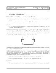
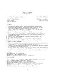
better understand and analyze a conflict when it occurs, we work with a subgraph of 

the implication graph, called the conflict graph (see Figure 2.1), that captures only one 

among possibly many ways of reaching a conflict from the decision variables using 

unit propagation. 

¬ p 

¬ q 

b 

a cut corresponding 

to clause (¬ a ∨ ¬ b) 

a 

¬ t 

¬ x 1 

¬ x 2 

¬ x 3 

reason side conflict side 

Figure 2.1: A conflict graph 

y 

¬ y 

conflict 

variable 

Definition 2. A conflict graph H is any subgraph of the implication graph with the 

following properties: 

(a) H contains Λ and exactly one conflict variable. 

(b) All nodes in H have a path to Λ. 

(c) Every node l in H other than Λ either corresponds to a decision literal or has 

precisely the nodes ¬l1,¬l2,...,¬lk as predecessors where (l1 ∨l2 ∨...∨lk ∨l) 

is a known clause. 

While an implication graph may or may not contain conflicts, a conflict graph 

always contains exactly one. The choice of the conflict graph is part of the strategy 

of the solver. A typical strategy will maintain one subgraph of an implication graph 

that has properties (b) and (c) from Definition 2, but not property (a). This can be 

Λ


thought of as a unique inference subgraph of the implication graph. When a conflict 

is reached, this unique inference subgraph is extended to satisfy property (a) as well, 

resulting in a conflict graph, which is then used to analyze the conflict. 

Conflict clauses 

For a subset U of the vertices of a graph, the edge-cut (henceforth called a cut) corresponding 

to U is the set of all edges going from vertices in U to vertices not in 

U. 

Consider the implication graph at a stage where there is a conflict and fix a conflict 

graph contained in that implication graph. Choose any cut in the conflict graph that 

has all decision variables on one side, called the reason side, and Λ as well as at least 

one conflict literal on the other side, called the conflict side. All nodes on the reason 

side that have at least one edge going to the conflict side form a cause of the conflict. 

The negations of the corresponding literals forms the conflict clause associated with 

this cut. 

Learning Schemes 

The essence of clause learning is captured by the learning scheme used to analyze and 

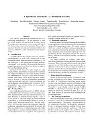
learn the “cause” of a failure. More concretely, different cuts in a conflict graph separating 

decision variables from a set of nodes containing Λ and a conflict literal correspond 

to different learning schemes (see Figure 2.2). One may also define learning 

schemes based on cuts not involving conflict literals at all such as a scheme suggested 

by Zhang et al. [240], but the effectiveness of such schemes is not clear. These will 

not be considered here. 

¬ p 

¬ q 

b 

Decision clause 

(p ∨ q ∨ ¬ b) 

a 

¬ t 

rel-sat clause 

(¬ a ∨ ¬ b) 

1UIP clause 

t 

¬ x 1 

¬ x 2 

¬ x3 FirstNewCut clause 

(x1 ∨ x2 ∨ x3) Figure 2.2: Learning schemes corresponding to different cuts in the conflict graph 

It is insightful to think of the nondeterministic scheme as the most general learning 

scheme. Here we select the cut nondeterministically, choosing, whenever possible, 

one whose associated clause is not already known. Since we can repeatedly 

branch on the same last variable, nondeterministic learning subsumes learning multiple 

clauses from a single conflict as long as the sets of nodes on the reason side of 

the corresponding cuts form a (set-wise) decreasing sequence. For simplicity, we will 

assume that only one clause is learned from any conflict. 

y 

¬ y 

Λ


In practice, however, we employ deterministic schemes. The decision scheme 

[240], for example, uses the cut whose reason side comprises all decision variables. 

Relsat [19] uses the cut whose conflict side consists of all implied variables at the 

current decision level. This scheme allows the conflict clause to have exactly one 

variable from the current decision level, causing an automatic flip in its assignment 

upon backtracking. In the example depicted in Figure 2.2, the decision clause (p ∨ 

q ∨ ¬b) has b as the only variable from the current decision level. After learning this 

conflict clause and backtracking by unassigning b, the truth values of p and q (both 

FALSE) immediately imply ¬b, flipping the value of b from TRUE to FALSE. 

This nice flipping property holds in general for all unique implication points 

(UIPs) [161]. A UIP of an implication graph is a node at the current decision level 

d such that every path from the decision variable at level d to the conflict variable or 

its negation must go through it. Intuitively, it is a single reason at level d that causes 

the conflict. Whereas relsat uses the decision variable as the obvious UIP, Grasp 

[161] and zChaff [170] use FirstUIP, the one that is “closest” to the conflict variable. 

Grasp also learns multiple clauses when faced with a conflict. This makes it typically 

require fewer branching steps but possibly slower because of the time lost in learning 

and unit propagation. 

The concept of UIP can be generalized to decision levels other than the current 

one. The 1UIP scheme corresponds to learning the FirstUIP clause of the current decision 

level, the 2UIP scheme to learning the FirstUIP clauses of both the current level 

and the one before, and so on. Zhang et al. [240] present a comparison of all these 

and other learning schemes and conclude that 1UIP is quite robust and outperforms 

all other schemes they consider on most of the benchmarks. 

Another learning scheme, which underlies the proof of a theorem to be presented 

in the next section, is the FirstNewCut scheme [22]. This scheme starts with the cut 

that is closest to the conflict literals and iteratively moves it back toward the decision 

variables until a conflict clause that is not already known is found; hence the name 

FirstNewCut. 

2.2.4 A Proof Complexity Perspective 

Propositional proof complexity is the study of the structure of proofs of validity of 

mathematical statements expressed in a propositional or Boolean form. Cook and 

Reckhow [52] introduced the formal notion of a proof system in order to study mathematical 

proofs from a computational perspective. They defined a propositional proof 

system to be an efficient algorithm A that takes as input a propositional statement S 

and a purported proof π of its validity in a certain pre-specified format. The crucial 

property of A is that for all invalid statements S, it rejects the pair (S,π) for all π, 

and for all valid statements S, it accepts the pair (S,π) for some proof π. This notion 

of proof systems can be alternatively formulated in terms of unsatisfiable formulas— 

those that are FALSE for all assignments to the variables. 

They further observed that if there is no propositional proof system that admits 

short (polynomial in size) proofs of validity of all tautologies, i.e., if there exist computationally 

hard tautologies for every propositional proof system, then the complexity 

classes NP and co-NP are different, and hence P = NP. This observation makes 

finding tautological formulas (equivalently, unsatisfiable formulas) that are computa-


tionally difficult for various proof systems one of the central tasks of proof complexity 

research, with far reaching consequences to complexity theory and Computer Science 

in general. These hard formulas naturally yield a hierarchy of proof systems based on 

the sizes of proofs they admit. Tremendous amount of research has gone into understanding 

this hierarchical structure. Beame and Pitassi [23] summarize many of the 

results obtained in this area. 

To understand current complete SAT solvers, we focus on the proof system called 

resolution, denoted henceforth as RES. It is a very simple system with only one rule 

which applies to disjunctions of propositional variables and their negations: (a OR B) 

and ((NOT a) OR C) together imply (B OR C). Repeated application of this rule 

suffices to derive an empty disjunction if and only if the initial formula is unsatisfiable; 

such a derivation serves as a proof of unsatisfiability of the formula. 

Despite its simplicity, unrestricted resolution as defined above (also called general 

resolution) is hard to implement efficiently due to the difficulty of finding good 

choices of clauses to resolve; natural choices typically yield huge storage requirements. 

Various restrictions on the structure of resolution proofs lead to less powerful 

but easier to implement refinements that have been studied extensively in proof complexity. 

Those of special interest to us are tree-like resolution, where every derived 

clause is used at most once in the refutation, and regular resolution, where every 

variable is resolved upon at most one in any “path” from the initial clauses to the 

empty clause. While these and other refinements are sound and complete as proof 

systems, they differ vastly in efficiency. For instance, in a series of results, Bonet 

et al. [34], Bonet and Galesi [35], and Buresh-Oppenheim and Pitassi [41] have shown 

that regular, ordered, linear, positive, negative, and semantic resolution are all exponentially 

stronger than tree-like resolution. On the other hand, Bonet et al. [34] and 

Alekhnovich et al. [7] have proved that tree-like, regular, and ordered resolution are 

exponentially weaker than RES. 

Most of today’s complete SAT solvers implement a subset of the resolution proof 

system. However, till recently, it wasn’t clear where exactly do they fit in the proof 

system hierarchy and how do they compare to refinements of resolution such as regular 

resolution. Clause learning and random restarts can be considered to be two 

of the most important ideas that have lifted the scope of modern SAT solvers from 

experimental toy problems to large instances taken from real world challenges. Despite 

overwhelming empirical evidence, for many years not much was known of the 

ultimate strengths and weaknesses of the two. 

Beame, Kautz, and Sabharwal [22, 199] answered several of these questions in a 

formal proof complexity framework. They gave the first precise characterization of 

clause learning as a proof system called CL and began the task of understanding its 

power by relating it to resolution. In particular, they showed that with a new learning 

scheme called FirstNewCut, clause learning can provide exponentially shorter proofs 

than any proper refinement of general resolution satisfying a natural self-reduction 

property. These include regular and ordered resolution, which are already known to 

be much stronger than the ordinary DPLL procedure which captures most of the SAT 

solvers that do not incorporate clause learning. They also showed that a slight variant 

of clause learning with unlimited restarts is as powerful as general resolution itself. 

From the basic proof complexity point of view, only families of unsatisfiable formulas 

are of interest because only proofs of unsatisfiability can be large; minimum


proofs of satisfiability are linear in the number of variables of the formula. In practice, 

however, many interesting formulas are satisfiable. To justify the approach of 

using a proof system CL, we refer to the work of Achlioptas, Beame, and Molloy [2] 

who have shown how negative proof complexity results for unsatisfiable formulas can 

be used to derive run time lower bounds for specific inference algorithms, especially 

DPLL, running on satisfiable formulas as well. The key observation in their work 

is that before hitting a satisfying assignment, an algorithm is very likely to explore 

a large unsatisfiable part of the search space that results from the first bad variable 

assignment. 

Proof complexity does not capture everything we intuitively mean by the power 

of a reasoning system because it says nothing about how difficult it is to find shortest 

proofs. However, it is a good notion with which to begin our analysis because 

the size of proofs provides a lower bound on the running time of any implementation 

of the system. In the systems we consider, a branching function, which determines 

which variable to split upon or which pair of clauses to resolve, guides the search. A 

negative proof complexity result for a system (“proofs must be large in this system”) 

tells us that a family of formulas is intractable even with a perfect branching function; 

likewise, a positive result (“small proofs exist”) gives us hope of finding a good 

branching function, i.e., a branching function that helps us uncover a small proof. 

We begin with an easy to prove relationship between DPLL (without clause learning) 

and tree-like resolution (for a formal proof, see e.g. [199]). 

Proposition 1. For a CNF formula F, the size of the smallest DPLL refutation of F is 

equal to the size of the smallest tree-like resolution refutation of F. 

The interesting part is to understand what happens when clause learning is brought 

into the picture. It has been previously observed by Lynce and Marques-Silva [157] 

that clause learning can be viewed as adding resolvents to a tree-like resolution proof. 

The following results show further that clause learning, viewed as a propositional 

proof system CL, is exponentially stronger than tree-like resolution. This explains, 

formally, the performance gains observed empirically when clause learning is added 

to DPLL based solvers. 

Clause Learning Proofs 

The notion of clause learning proofs connects clause learning with resolution and 

provides the basis for the complexity bounds to follow. If a given formula F is unsatisfiable, 

the clause learning based DPLL process terminates with a conflict at decision 

level zero. Since all clauses used in this final conflict themselves follow directly or 

indirectly from F, this failure of clause learning in finding a satisfying assignment 

constitutes a logical proof of unsatisfiability of F. In an informal sense, we denote by 

CL the proof system consisting of all such proofs; this can be made precise using the 

notion of a branching sequence [22]. The results below compare the sizes of proofs in 

CL with the sizes of (possibly restricted) resolution proofs. Note that clause learning 

algorithms can use one of many learning schemes, resulting in different proofs. 

We next define what it means for a refinement of a proof system to be natural and 

proper. Let CS(F) denote the length of a shortest refutation of a formula F under a 

proof system S.


Definition 3 ([22, 199]). For proof systems S and T , and a function f : N → [1,∞), 

• S is natural if for any formula F and restriction ρ on its variables, CS(F|ρ) ≤ 

CS(F). 

• S is a refinement of T if proofs in S are also (restricted) proofs in T . 

• S is f (n)-proper as a refinement of T if there exists a witnessing family {Fn} 

of formulas such that CS(Fn) ≥ f (n) · CT (Fn). The refinement is exponentiallyproper 

if f (n) = 2 nΩ(1) 

and super-polynomially-proper if f (n) = n ω(1) . 

Under this definition, tree-like, regular, linear, positive, negative, semantic, and 

ordered resolution are natural refinements of RES, and further, tree-like, regular, and 

ordered resolution are exponentially-proper [7, 34]. 

Now we are ready to state the somewhat technical theorem relating the clause 

learning process to resolution, whose corollaries are nonetheless easy to understand. 

The proof of this theorem is based on an explicit construction of so-called “proof-trace 

extension” formulas, which interestingly allow one to translate any known separation 

result between RES and a natural proper refinement S of RES into a separation between 

CL and S. 

Theorem 1 ([22, 199]). For any f (n)-proper natural refinement S of RES and for CL 

using the FirstNewCut scheme and no restarts, there exist formulas {Fn} such that 

CS(Fn) ≥ f (n) · CCL(Fn). 

Corollary 1. CL can provide exponentially shorter proofs than tree-like, regular, and 

ordered resolution. 

Corollary 2. Either CL is not a natural proof system or it is equivalent in strength to 

RES. 

We remark that this leaves open the possibility that CL may not be able to simulate 

all regular resolution proofs. In this context, MacKenzie [158] has used arguments 

similar to those of Beame et al. [20] to prove that a natural variant of clause learning 

can indeed simulate all of regular resolution. 

Finally, let CL-- denote the variant of CL where one is allowed to branch on a literal 

whose value is already set explicitly or because of unit propagation. Of course, such 

a relaxation is useless in ordinary DPLL; there is no benefit in branching on a variable 

that doesn’t even appear in the residual formula. However, with clause learning, such 

a branch can lead to an immediate conflict and allow one to learn a key conflict clause 

that would otherwise have not been learned. This property can be used to prove that 

RES can be efficiently simulated by CL-- with enough restarts. In this context, a clause 

learning scheme will be called non-redundant if on a conflict, it always learns a clause 

not already known. Most of the practical clause learning schemes are non-redundant. 

Theorem 2 ([22, 199]). CL-- with any non-redundant scheme and unlimited restarts 

is polynomially equivalent to RES. 

We note that by choosing the restart points in a smart way, CL together with 

restarts can be converted into a complete algorithm for satisfiability testing, i.e., for


all unsatisfiable formulas given as input, it will halt and provide a proof of unsatisfiability 

[16, 102]. The theorem above makes a much stronger claim about a slight 

variant of CL, namely, with enough restarts, this variant can always find proofs of 

unsatisfiability that are as short as those of RES. 

2.2.5 Symmetry Breaking 

One aspect of many theoretical as well as real-world problems that merits attention is 

the presence of symmetry or equivalence amongst the underlying objects. Symmetry 

can be defined informally as a mapping of a constraint satisfaction problem (CSP) 

onto itself that preserves its structure as well as its solutions. The concept of symmetry 

in the context of SAT solvers and in terms of higher level problem objects is 

best explained through some examples of the many application areas where it naturally 

occurs. For instance, in FPGA (field programmable gate array) routing used 

in electronics design, all available wires or channels used for connecting two switch 

boxes are equivalent; in our design, it does not matter whether we use wire #1 between 

connector X and connector Y, or wire #2, or wire #3, or any other available 

wire. Similarly, in circuit modeling, all gates of the same “type” are interchangeable, 

and so are the inputs to a multiple fan-in AND or OR gate (i.e., a gate with several inputs); 

in planning, all identical boxes that need to be moved from city A to city B are 

equivalent; in multi-processor scheduling, all available processors are equivalent; in 

cache coherency protocols in distributed computing, all available identical caches are 

equivalent. A key property of such objects is that when selecting k of them, we can 

choose, without loss of generality, any k. This without-loss-of-generality reasoning is 

what we would like to incorporate in an automatic fashion. 

The question of symmetry exploitation that we are interested in addressing arises 

when instances from domains such as the ones mentioned above are translated into 

CNF formulas to be fed to a SAT solver. A CNF formula consists of constraints over 

different kinds of variables that typically represent tuples of these high level objects 

(e.g. wires, boxes, etc.) and their interaction with each other. For example, during 

the problem modeling phase, we could have a Boolean variable zw,c that is TRUE iff 

the first end of wire w is attached to connector c. When this formula is converted 

into DIMACS format for a SAT solver, the semantic meaning of the variables, that, 

say, variable 1324 is associated with wire #23 and connector #5, is discarded. Consequently, 

in this translation, the global notion of the obvious interchangeability of 

the set of wire objects is lost, and instead manifests itself indirectly as a symmetry 

between the (numbered) variables of the formula and therefore also as a symmetry 

within the set of satisfying (or un-satisfying) variable assignments. These sets of 

symmetric satisfying and un-satisfying assignments artificially explode both the satisfiable 

and the unsatisfiable parts of the search space, the latter of which can be a 

challenging obstacle for a SAT solver searching for a satisfying assignment. 

One of the most successful techniques for handling symmetry in both SAT and 

general CSPs originates from the work of Puget [187], who showed that symmetries 

can be broken by adding one lexicographic ordering constraint per symmetry. 

Crawford et al. [55] showed how this can be done by adding a set of simple “lexconstraints” 

or symmetry breaking predicates (SBPs) to the input specification to 

weed out all but the lexically-first solutions. The idea is to identify the group of


permutations of variables that keep the CNF formula unchanged. For each such permutation 

π, clauses are added so that for every satisfying assignment σ for the original 

problem, whose permutation π(σ) is also a satisfying assignment, only the lexicallyfirst 

of σ and π(σ) satisfies the added clauses. In the context of CSPs, there has been 

a lot of work in the area of SBPs. Petrie and Smith [182] extended the idea to value 

symmetries, Puget [189] applied it to products of variable and value symmetries, and 

Walsh [231] generalized the concept to symmetries acting simultaneously on variables 

and values, on set variables, etc. Puget [188] has recently proposed a technique 

for creating dynamic lex-constraints, with the goal of minimizing adverse interaction 

with the variable ordering used in the search tree. 

In the context of SAT, value symmetries for the high-level variables naturally manifest 

themselves as low-level variable symmetries, and work on SBPs has taken a 

different path. Tools such as Shatter by Aloul et al. [8] improve upon the basic 

SBP technique by using lex-constraints whose size is only linear in the number of 

variables rather than quadratic. Further, they use graph isomorphism detectors like 

Saucy by Darga et al. [56] to generate symmetry breaking predicates only for the 

generators of the algebraic groups of symmetry. This latter problem of computing 

graph isomorphism, however, is not known to have any polynomial time algorithms, 

and is conjectured to be strictly between the complexity classes P and NP [cf. 136]. 

Hence, one must resort to heuristic or approximate solutions. Further, while there are 

formulas for which few SBPs suffice, the number of SBPs one needs to add in order 

to break all symmetries can be exponential. This is typically handled in practice by 

discarding “large” symmetries, i.e., those involving too many variables with respect to 

a fixed threshold. This may, however, sometimes result in much slower SAT solutions 

in domains such as clique coloring and logistics planning. 

A very different and indirect approach for addressing symmetry is embodied in 

SAT solvers such as PBS by Aloul et al. [9], pbChaff by Dixon et al. [68], and 

Galena by Chai and Kuehlmann [44], which utilize non-CNF formulations known 

as pseudo-Boolean inequalities. Their logic reasoning is based on what is called the 

Cutting Planes proof system which, as shown by Cook et al. [53], is strictly stronger 

than resolution on which DPLL type CNF solvers are based. Since this more powerful 

proof system is difficult to implement in its full generality, pseudo-Boolean solvers 

often implement only a subset of it, typically learning only CNF clauses or restricted 

pseudo-Boolean constraints upon a conflict. Pseudo-Boolean solvers may lead to 

purely syntactic representational efficiency in cases where a single constraint such as 

y1 + y2 + ... + yk ≤ 1 is equivalent to k 2 binary clauses. More importantly, they are 

relevant to symmetry because they sometimes allow implicit encoding. For instance, 

the single constraint x1 +x2 +...+xn ≤ m over n variables captures the essence of the 

pigeonhole formula PHPn m over nm variables which is provably exponentially hard to 

solve using resolution-based methods without symmetry considerations [108]. This 

implicit representation, however, is not suitable in certain applications such as clique 

coloring and planning that we discuss. In fact, for unsatisfiable clique coloring instances, 

even pseudo-Boolean solvers provably require exponential time. 

One could conceivably keep the CNF input unchanged but modify the solver to 

detect and handle symmetries during the search phase as they occur. Although this 

approach is quite natural, we are unaware of its implementation in a general purpose 

SAT solver besides sEqSatz by Li et al. [151], which has been shown to be effective


on matrix multiplication and polynomial multiplication problems. Symmetry handling 

during search has been explored with mixed results in the CSP domain using 

frameworks like SBDD and SBDS [e.g. 72, 73, 84, 87]. Related work in SAT has 

been done in the specific areas of automatic test pattern generation by Marques-Silva 

and Sakallah [162] and SAT-based model checking by Shtrichman [214]. In both 

cases, the solver utilizes global information obtained at a stage to make subsequent 

stages faster. In other domain-specific work on symmetries in problems relevant to 

SAT, Fox and Long [74] propose a framework for handling symmetry in planning 

problems solved using the planning graph framework. They detect equivalence between 

various objects in the planning instance and use this information to reduce the 

search space explored by their planner. Unlike typical SAT-based planners, this approach 

does not guarantee plans of optimal length when multiple (non-conflicting) 

actions are allowed to be performed at each time step in parallel. Fortunately, this 

issue does not arise in the SymChaff approach for SAT to be mentioned shortly. 

Dixon et al. [67] give a generic method of representing and dynamically maintaining 

symmetry in SAT solvers using algebraic techniques that guarantee polynomial 

size unsatisfiability proofs of many difficult formulas. The strength of their work lies 

in a strong group theoretic foundation and comprehensiveness in handling all possible 

symmetries. The computations involving group operations that underlie their current 

implementation are, however, often quite expensive. 

When viewing complete SAT solvers as implementations of proof systems, the 

challenge with respect to symmetry exploitation is to push the underlying proof system 

up in the weak-to-strong proof complexity hierarchy without incurring the significant 

cost that typically comes from large search spaces associated with complex proof 

systems. While most of the current SAT solvers implement subsets of the resolution 

proof system, a different kind of solver called SymChaff [199, 200] brings it up closer 

to symmetric resolution, a proof system known to be exponentially stronger than resolution 

[139, 226]. More critically, it achieves this in a time- and space-efficient 

manner. Interestingly, while SymChaff involves adding structure to the problem description, 

it still stays within the realm of SAT solvers (as opposed to using a constraint 

programming (CP) approach), thereby exploiting the many benefits of the CNF form 

and the advances in state-of-the-art SAT solvers. 

As a structure-aware solver, SymChaff incorporates several new ideas, including 

simple but effective symmetry representation, multiway branching based on variable 

classes and symmetry sets, and symmetric learning as an extension of clause learning 

to multiway branches. Two key places where it differs from earlier approaches are 

in using high level problem description to obtain symmetry information (instead of 

trying to recover it from the CNF formula) and in maintaining this information dynamically 

but without using a complex group theoretic machinery. This allows it to 

overcome many drawbacks of previously proposed solutions. It is shown, in particular, 

that straightforward annotation in the usual PDDL specification of planning problems 

is enough to automatically and quickly generate relevant symmetry information, 

which in turn makes the search for an optimal plan several orders of magnitude faster. 

Similar performance gains are seen in other domains as well.


2.3 SAT Solver Technology—Incomplete Methods 

An incomplete method for solving the SAT problem is one that does not provide 

the guarantee that it will eventually either report a satisfying assignment or prove 

the given formula unsatisfiable. Such a method is typically run with a pre-set limit, 

after which it may or may not produce a solution. Unlike the systematic solvers 

based on an exhaustive branching and backtracking search, incomplete methods are 

generally based on stochastic local search. On problems from a variety of domains, 

such incomplete methods for SAT can significantly outperform DPLL-based methods. 

Since the early 1990’s, there has been a tremendous amount of research on designing, 

understanding, and improving local search methods for SAT [e.g. 43, 77, 88, 89, 

104, 105, 109, 113, 114, 116, 132, 137, 152, 164, 180, 183, 191, 206, 219] as well 

as on hybrid approaches that attempt to combine DPLL and local search methods 

[e.g. 10, 106, 163, 185, 195]. 5 We begin this section by discussing two methods 

that played a key role in the success of local search in SAT, namely GSAT [213] and 

Walksat [211]. We will then explore the phase transition phenomenon in random 

SAT and a relatively new incomplete technique called Survey Propagation. We note 

that there are also other exciting related solution techniques such as those based on 

Lagrangian methods [207, 229, 235] and translation to integer programming [112, 

124]. 

The original impetus for trying a local search method on satisfiability problems 

was the successful application of such methods for finding solutions to large N-queens 

problems, first using a connectionist system by Adorf and Johnston [6], and then using 

greedy local search by Minton et al. [167]. It was originally assumed that this 

success simply indicated that N-queens was an easy problem, and researchers felt that 

such techniques would fail in practice for SAT. In particular, it was believed that local 

search methods would easily get stuck in local minima, with a few clauses remaining 

unsatisfied. The GSAT experiments showed, however, that certain local search strategies 

often do reach global minima, in many cases much faster than systematic search 

strategies. 

GSAT is based on a randomized local search technique [153, 177]. The basic GSAT 

procedure, introduced by Selman et al. [213] and described here as Algorithm 2.3, 

starts with a randomly generated truth assignment. It then greedily changes (‘flips’) 

the assignment of the variable that leads to the greatest decrease in the total number 

of unsatisfied clauses. Such flips are repeated until either a satisfying assignment is 

found or a pre-set maximum number of flips (MAX-FLIPS) is reached. This process is 

repeated as needed, up to a maximum of MAX-TRIES times. 

Selman et al. showed that GSAT substantially outperformed even the best backtracking 

search procedures of the time on various classes of formulas, including randomly 

generated formulas and SAT encodings of graph coloring problems [123]. The 

search of GSAT typically begins with a rapid greedy descent towards a better assignment, 

followed by long sequences of “sideways” moves, i.e., moves that do not increase 

or decrease the total number of unsatisfied clauses. In the search space, each 

collection of truth assignments that are connected together by a sequence of possible 

5 As in our discussion of the complete SAT solvers, we cannot do justice to all recent research in local 

search solvers for SAT. We will again try to provide a brief overview and touch upon some interesting 

details.


Algorithm 2.3: GSAT (F) 

Input : A CNF formula F 

Parameters : Integers MAX-FLIPS, MAX-TRIES 

Output : A satisfying assignment for F, or FAIL 

begin 

for i ← 1 to MAX-TRIES do 

σ ← a randomly generated truth assignment for F 

for j ← 1 to MAX-FLIPS do 

if σ satisfies F then return σ // success 

v ← a variable flipping which results in the greatest decrease 

(possibly negative) in the number of unsatisfied clauses 

Flip v in σ 

return FAIL // no satisfying assignment found 

end 

sideways moves is referred to as a plateau. Experiments indicate that on many formulas, 

GSAT spends most of its time moving from plateau to plateau. Interestingly, 

Frank et al. [77] observed that in practice, almost all plateaus do have so-called “exits” 

that lead to another plateau with a lower number of unsatisfied clauses. Intuitively, 

in a very high dimensional search space such as the space of a 10,000 variable formula, 

it is very rare to encounter local minima, which are plateaus from where there 

is no local move that decreases the number of unsatisfied clauses. In practice, this 

means that GSAT most often does not get stuck in local minima, although it may take 

a substantial amount of time on each plateau before moving on to the next one. This 

motivates studying various modifications in order to speed up this process [209, 210]. 

One of the most successful strategies is to introduce noise into the search in the form 

of uphill moves, which forms the basis of the now well-known local search method 

for SAT called Walksat [211]. 

Walksat interleaves the greedy moves of GSAT with random walk moves of a 

standard Metropolis search. It further focuses the search by always selecting the variable 

to flip from an unsatisfied clause C (chosen at random). If there is a variable in C 

flipping which does not turn any currently satisfied clauses to unsatisfied, it flips this 

variable (a “freebie” move). Otherwise, with a certain probability, it flips a random 

literal of C (a “random walk” move), and with the remaining probability, it flips a 

variable in C that minimizes the break-count, i.e., the number of currently satisfied 

clauses that become unsatisfied (a “greedy” move). Walksat is presented in detail 

as Algorithm 2.4. One of its parameters, in addition to the maximum number of tries 

and flips, is the noise p ∈ [0,1], which controls how often are non-greedy moves considered 

during the stochastic search. It has been found empirically that for various 

problems from a single domain, a single value of p is optimal. 

The focusing strategy of Walksat based on selecting variables solely from unsatisfied 

clauses was inspired by the O(n 2 ) randomized algorithm for 2-SAT by Papadimitriou 

[178]. It can be shown that for any satisfiable formula and starting from 

any truth assignment, there exists a sequence of flips using only variables from unsatisfied 

clauses such that one obtains a satisfying assignment.

Algorithm 2.4: Walksat (F) 


Input : A CNF formula F 

Parameters : Integers MAX-FLIPS, MAX-TRIES; noise parameter p ∈ [0,1] 

Output : A satisfying assignment for F, or FAIL 

begin 

for i ← 1 to MAX-TRIES do 

σ ← a randomly generated truth assignment for F 

for j ← 1 to MAX-FLIPS do 

if σ satisfies F then return σ // success 

C ← an unsatisfied clause of F chosen at random 

if ∃ variable x ∈ C with break-count = 0 then 

v ← x // freebie move 

else 

With probability p: // random walk move 

v ← a variable in C chosen at random 

With probability 1 − p: // greedy move 

v ← a variable in C with the smallest break-count 

Flip v in σ 

return FAIL // no satisfying assignment found 

end 

When one compares the biased random walk strategy of Walksat on hard random 

3-CNF formulas against basic GSAT, the simulated annealing process of Kirkpatrick 

et al. [131], and a pure random walk strategy, the biased random walk process significantly 

outperforms the other methods [210]. In the years following the development 

of Walksat, many similar methods have been shown to be highly effective on not 

only random formulas but on many classes of structured instances, such as encodings 

of circuit design problems, Steiner tree problems, problems in finite algebra, and AI 

planning [cf. 116]. Various extensions of the basic process have also been explored, 

such as dynamic search policies like adapt-novelty [114], incorporating unit 

clause elimination as in the solver UnitWalk [109], and exploiting problem structure 

for increased efficiency [183]. Recently, it was shown that the performance of 

stochastic solvers on many structured problems can be further enhanced by using new 

SAT encodings that are designed to be effective for local search [186]. 

2.3.1 The Phase Transition Phenomenon in Random k-SAT 

One of the key motivations in the early 1990’s for studying incomplete, stochastic 

methods for solving SAT problems was the finding that DPLL-based systematic 

solvers perform quite poorly on certain randomly generated formulas. Consider a random 

k-CNF formula F on n variables generated by independently creating m clauses 

as follows: for each clause, select k distinct variables uniformly at random out of the 

n variables and negate each variable with probability 0.5. When F is chosen from this 

distribution, Mitchell, Selman, and Levesque [168] observed that the median hardness 

of the problems is very nicely characterized by a key parameter: the clause-tovariable 

ratio, m/n, typically denoted by α. They observed that problem hardness


peaks in a critically constrained region determined by α alone. The left pane of Figure 

2.3 depicts the now well-known “easy-hard-easy” pattern of SAT and other combinatorial 

problems, as the key parameter (in this case α) is varied. For random 3-SAT, 

this region has been experimentally shown to be around α ≈ 4.26 (see [54, 132] for 

early results), and has provided challenging benchmarks as a test-bed for SAT solvers. 

Cheeseman et al. [45] observed a similar easy-hard-easy pattern in random graph coloring 

problems. For random formulas, interestingly, a slight natural variant of the 

above “fixed-clause-length” model, called the variable-clause-length model, does not 

have a clear set of parameters that leads to a hard set of instances [76, 92, 190]. This 

apparent difficulty in generating computationally hard instances for SAT solvers provided 

the impetus for much of the early work on local search methods for SAT. We 

refer the reader to [50] for a nice survey. 

# of DP calls 

4000 

3500 

3000 

2500 

2000 

1500 

1000 

500 

20--variable formulas 



0 

2 3 4 5 6 

Ratio of clauses-to-variables 

7 8 

Fraction of unsatisfiable formulae 

1 

0.8 

0.6 

0.4 

0.2 

Threshold for 3SAT 

N = 12 

N = 20 

N = 24 

N = 40 

N = 50 

N = 100 

0 

3 3.5 4 4.5 5 

M/N 

5.5 6 6.5 7 

Figure 2.3: The phase transition phenomenon in random 3-SAT. Left: Computational 

hardness peaks at α ≈ 4.26. Right: Problems change from being mostly satisfiable to 

mostly unsatisfiable. The transitions sharpen as the number of variables grows. 

This critically constrained region marks a stark transition not only in the computational 

hardness of random SAT instances but also in their satisfiability itself. The 

right pane of Figure 2.3 shows the fraction of random formulas that are unsatisfiable, 

as a function of α. We see that nearly all problems with α below the critical region 

(the under-constrained problems) are satisfiable. As α approaches and passes the critical 

region, there is a sudden change and nearly all problems in this over-constrained 

region are unsatisfiable. Further, as n grows, this phase transition phenomenon becomes 

sharper and sharper, and coincides with the region in which the computational 

hardness peaks. The relative hardness of the instances in the unsatisfiable region to 

the right of the phase transition is consistent with the formal result of Chvátal and 

Szemerédi [48] who, building upon the work of Haken [108], proved that large unsatisfiable 

random k-CNF formulas almost surely require exponential size resolution 

refutations, and thus exponential length runs of any DPLL-based algorithm proving 

unsatisfiability. This formal result was subsequently refined and strengthened by others 

[cf. 21, 24, 49]. 

Relating the phase transition phenomenon for 3-SAT to statistical physics, Kirkpatrick 

and Selman [132] showed that the threshold has characteristics typical of 

phase transitions in the statistical mechanics of disordered materials (see also [169]). 

Physicists have studied phase transition phenomena in great detail because of the


many interesting changes in a system’s macroscopic behavior that occur at phase 

boundaries. One useful tool for the analysis of phase transition phenomena is called 

finite-size scaling analysis. This approach is based on rescaling the horizontal axis 

by a factor that is a function of n. The function is such that the horizontal axis is 

stretched out for larger n. In effect, rescaling “slows down” the phase-transition for 

higher values of n, and thus gives us a better look inside the transition. From the resulting 

universal curve, applying the scaling function backwards, the actual transition 

curve for each value of n can be obtained. In principle, this approach also localizes 

the 50%-satisfiable-point for any value of n, which allows one to generate the hardest 

possible random 3-SAT instances. 

Interestingly, it is still not formally known whether there even exists a critical constant 

αc such that as n grows, almost all 3-SAT formulas with α < αc are satisfiable 

and almost all 3-SAT formulas with α > αc are unsatisfiable. In this respect, Friedgut 

[78] provided the first positive result, showing that there exists a function αc(n) depending 

on n such that the above threshold property holds. (It is quite likely that the 

threshold in fact does not depend on n, and is a fixed constant.) In a series of papers, 

researchers have narrowed down the gap between upper bounds on the threshold for 

3-SAT [e.g. 40, 69, 76, 120, 133], the best so far being 4.596, and lower bounds [e.g. 

1, 5, 40, 75, 79, 107, 125], the best so far being 3.52. On the other hand, for random 

2-SAT, we do have a full rigorous understanding of the phase transition, which occurs 

at clause-to-variable ratio of 1 [33, 47]. Also, for general k, the threshold for random 

k-SAT is known to be in the range 2 k ln2 − O(k) [3, 101]. 

2.3.2 A New Technique for Random k-SAT: Survey Propagation 

We end this section with a brief discussion of Survey Propagation (SP), an exciting 

new algorithm for solving hard combinatorial problems. It was discovered in 2002 by 

Mézard, Parisi, and Zecchina [165], and is so far the only known method successful at 

solving random 3-SAT instances with one million variables and beyond in near-linear 

time in the most critically constrained region. 6 

The SP method is quite radical in that it tries to approximate, using an iterative 

process of local “message” updates, certain marginal probabilities related to the set 

of satisfying assignments. It then assigns values to variables with the most extreme 

probabilities, simplifies the formula, and repeats the process. This strategy is referred 

to as SP-inspired decimation. In effect, the algorithm behaves like the usual DPLLbased 

methods, which also assign variable values incrementally in an attempt to find a 

satisfying assignment. However, quite surprisingly, SP almost never has to backtrack. 

In other words, the “heuristic guidance” from SP is almost always correct. Note that, 

interestingly, computing marginals on satisfying assignments is strongly believed to 

be much harder than finding a single satisfying assignment (#P-complete vs. NPcomplete). 

Nonetheless, SP is able to efficiently approximate certain marginals on 

random SAT instances and uses this information to successfully find a satisfying assignment. 

SP was derived from rather complex statistical physics methods, specifically, the 

so-called cavity method developed for the study of spin glasses. The method is still far 

6 It has been recently shown that by finely tuning the noise parameter, Walksat can also be made to 

scale well on hard random 3-SAT instances, well above the clause-to-variable ratio of 4.2 [208].


from well-understood, but in recent years, we are starting to see results that provide 

important insights into its workings [e.g. 4, 12, 39, 140, 159, 166]. Close connections 

to belief propagation (BP) methods [181] more familiar to computer scientists have 

been subsequently discovered. In particular, it was shown by Braunstein and Zecchina 

[39] (later extended by Maneva, Mossel, and Wainwright [159]) that SP equations are 

equivalent to BP equations for obtaining marginals over a special class of combinatorial 

objects, called covers. In this respect, SP is the first successful example of the use 

of a probabilistic reasoning technique to solve a purely combinatorial search problem. 

The recent work of Kroc et al. [140] empirically established that SP, despite the very 

loopy nature of random formulas which violate the standard tree-structure assumptions 

underlying the BP algorithm, is remarkably good at computing marginals over 

these covers objects on large random 3-SAT instances. 

Unfortunately, the success of SP is currently limited to random SAT instances. It 

is an exciting research challenge to further understand SP and apply it successfully to 

more structured, real-world problem instances. 

2.4 Runtime Variance and Problem Structure 

The performance of backtrack-style search methods can vary dramatically depending 

on the way one selects the next variable to branch on (the “variable selection heuristic”) 

and in what order the possible values are assigned to the variable (the “value 

selection heuristic”). The inherent exponential nature of the search process appears 

to magnify the unpredictability of search procedures. In fact, it is not uncommon to 

observe a backtrack search procedure “hang” on a given instance, whereas a different 

heuristic, or even just another randomized run, solves the instance quickly. A related 

phenomenon is observed in random problem distributions that exhibit an “easy-hardeasy” 

pattern in computational complexity, concerning so-called “exceptionally hard” 

instances: such instances seem to defy the “easy-hard-easy” pattern. They occur in 

the under-constrained area, but they seem to be considerably harder than other similar 

instances and even harder than instances from the critically constrained area. This 

phenomenon was first identified by Hogg and Willimans in graph coloring [111] and 

by Gent and Walsh in satisfiability problems [83]. An instance is considered to be exceptionally 

hard, for a particular search algorithm, when it occurs in the region where 

almost all problem instances are satisfiable (i.e., the under constrained area), but is 

considerably harder to solve than other similar instances, and even harder than most 

of the instances in the critically constrained area [83, 111, 217]. However, subsequent 

research showed that such instances are not inherently difficult; for example, 

by simply renaming the variables or by considering a different search heuristic such 

instances can be easily solved [212, 218]. Therefore, the “hardness” of exceptionally 

hard instances does not reside in the instances per se, but rather in the combination 

of the instance with the details of the search method. This is the reason why 

researchers studying the hardness of computational problems use the median to characterize 

search difficulty, instead of the mean, since the behavior of the mean tends to 

be quite erratic [95].

2.4.1 Fat and Heavy Tailed behavior 


The study of the full runtime distributions of search methods—instead of just the moments 

and median—has been shown to provide a better characterization of search 

methods and much useful information in the design of algorithms. In particular, 

researchers have shown that the runtime distributions of complete backtrack search 

methods reveal intriguing characteristics of such search methods: quite often complete 

backtrack search methods exhibit fat and heavy-tailed behavior [80, 95, 111]. 

Such runtime distributions can be observed when running a deterministic backtracking 

procedure on a distribution of random instances, and perhaps more importantly 

by repeated runs of a randomized backtracking procedure on a single instance. 

The notion of fat-tailedness is based on the concept of kurtosis. The kurtosis 

is defined as µ4/µ 2 2 (µ4 is the fourth central moment about the mean and µ2 is the 

second central moment about the mean, i.e., the variance). If a distribution has a high 

central peak and long tails, than the kurtosis is in general large. The kurtosis of the 

standard normal distribution is 3. A distribution with a kurtosis larger than 3 is fattailed 

or leptokurtic. Examples of distributions that are characterized by fat-tails are 

the exponential distribution, the lognormal distribution, and the Weibull distribution. 

Heavy-tailed distributions have “heavier” tails than fat-tailed distributions; in fact 

they have some infinite moments, e.g., they can have infinite mean, infinite variance, 

etc. More rigorously, a random variable X with probability distribution function F(·) 

is heavy-tailed if it has the so-called Pareto like decay of the tails, i.e.: 

1 − F(x) = Pr[X > x] ∼ Cx −α , x > 0, 

where α > 0 and C > 0 are constants. When 1 < α < 2, X has infinite variance, 

and infinite mean and variance when 0 < α


as sub-solver, that solves a tractable sub-case of the general constraint satisfaction 

problem [233]. 

Definition 4. A sub-solver A given as input a CSP, C, satisfies the following: 

i. Trichotomy: A either rejects the input C, or “determines” C correctly (as unsatisfiable 

or satisfiable, returning a solution if satisfiable), 

ii. Efficiency: A runs in polynomial time, 

iii. Trivial solvability: A can determine if C is trivially true (has no constraints) or 

trivially false (has a contradictory constraint), 

iv. Self-reducibility: if A determines C, then for any variable x and value v, A determines 

C[v/x]. 7 

For instance, A could be an algorithm that enforces arc consistency. Using the 

definition of sub-solver we can now formally define the concept of backdoor set. Let 

A be a sub-solver and C be a CSP. A nonempty subset S of the variables with domain 

D is a (weak) backdoor in C for A if for some aS : S → D, A returns a satisfying 

assignment of C[aS]. Intuitively, the backdoor corresponds to a set of variables, such 

that when set correctly, the sub-solver can solve the remaining problem. A stronger 

notion of backdoors considers both satisfiable and unsatisfiable (inconsistent) problem 

instances. A nonempty subset S of the variables is a strong backdoor in C for A if for 

all aS : S → D, A returns a satisfying assignment or concludes unsatisfiability of C[aS]. 

Szeider [223] considered the parameterized complexity of the problem of determining 

whether a SAT instance has a weak or strong backdoor set of size k or less for 

DPLL style sub-solvers, i.e., subsolvers based on unit propagation and/or pure literal 

elimination. He showed that detection of weak and strong backdoor sets is unlikely to 

be fixed-parameter tractable. Nishimura et al. [172] provided more positive results for 

detecting backdoor sets where the sub-solver solves Horn or 2-CNF formulas, both 

of which are linear time problems. They proved that the detection of such a strong 

backdoor set is fixed-parameter tractable, while the detection of a weak backdoor set 

is not. The explanation that they offered for such a discrepancy is quite interesting: 

for strong backdoor sets one only has to guarantee that the chosen set of variables 

gives a subproblem within the chosen syntactic class; for weak backdoor sets, one 

also has to guarantee satisfiability of the simplified formula, a property that cannot be 

described syntactically. 

Dilkina et al. [66] studied the tradeoff between the complexity of backdoor detection 

and the backdoor size. They proved that adding certain obvious inconsistency 

checks to the underlying class can make the complexity of backdoor detection jump 

from being within NP to being both NP-hard and coNP-hard. On the positive side, 

they showed that this change can dramatically reduce the size of the resulting backdoors. 

They also explored the differences between so-called deletion backdoors and 

strong backdoors, in particular with respect to the class of renamable Horn formulas. 

Concerning the size of backdoors, random formulas do not appear to have small 

backdoor sets. For example, for random 3-SAT problems near the phase transition, 

the backdoor size appears to be a constant fraction (roughly 30%) of the total number 

7 We use C[v/x] to denote the simplified CSP obtained by setting the value of variable x to v in C.


of variables [119]. This may explain why the current DPLL based solvers have not 

made significant progress on hard randomly generated instances. Empirical results 

based on real-world instances suggest a more positive picture. Structured problem 

instances can have surprisingly small sets of backdoor variables, which may explain 

why current state-of-the-art solvers are able to solve very large real-world instances. 

For example the logistics-d planning problem instance (log.d) has a backdoor set of 

just 12 variables, compared to a total of nearly 7,000 variables in the formula, using 

the polynomial time propagation techniques of the SAT solver Satz [148]. Hoffmann 

et al. [110] proved the existence of strong backdoor sets of size just O(logn) for 

certain families of logistics planning problems and blocks world problems. 

Figure 2.4: Constraint graph of a real-world instance from the logistics planning domain. 

The instance in the plot has 843 vars and 7,301 clauses. One backdoor set for 

this instance w.r.t. unit propagation has size 16 (not necessarily the minimum backdoor 

set). Left: Constraint graph of the original instance. Center: Constraint graph 

after setting 5 variables and performing unit propagation. Right: Constraint graph 

after setting 14 variables and performing unit propagation. 

Even though computing minimum backdoor sets is worst-case intractable [223], if 

we bound the size of the backdoor, heuristics and techniques like randomization and 

restarts can often uncover a small backdoor in practice [130]. In fact, state-of-theart 

SAT solvers are surprisingly effective in finding small backdoors in many structured 

problem instances. Figure 2.4 shows a visualization of the constraint graph of 

a logistics planning problem and how this graph is drastically simplified after only 

a few variables occurring in a small backdoor (found by SAT solvers) are set. In 

related work, Slaney and Walsh [216] studied the structural notion of “backbones” 

and Dequen and Dubois introduced a heuristic for DPLL based solvers that exploits 

the notion of backbone and outperforms other heuristics on random 3-SAT problems 

[65, 70]. 

2.4.3 Restarts 

One way to exploit heavy-tailed behavior is to add restarts to a backtracking procedure. 

A sequence of short runs instead of a single long run may be a more effective use 

of computational resources (see Figure 2.5). Gomes et al. proposed randomized rapid 

restarts (RRR) to take advantage of heavy-tailed behavior and boost the efficiency of


complete backtrack search procedures [102]. In practice, one gradually increases the 

cutoff to maintain completeness [16, 102]. Gomes et al. showed that a restart strategy 

with a fixed cutoff eliminates heavy-tail behavior and has finite moments [96]. 

Prior to the discovery of heavy-tailed behavior and backdoor sets, randomized 

restart policies have been studied in the context of general randomized Las Vegas 

procedures. Luby et al. [155] showed that when the underlying runtime distribution 

of the randomized procedure is fully known, the optimal restart policy is a fixed cutoff. 

When there is no a priori knowledge about the distribution, they also provided 

a universal strategy which minimizes the expected cost. This consists of runs whose 

lengths are powers of two, and each time a pair of runs of a given length has been 

completed, a run of twice that length is immediately executed. The universal strategy 

is of the form: 1,1,2,1,1,2,4,1,1,2,4,8,···. Although the universal strategy of Luby 

et al. is provably within a log factor of the optimal fixed cutoff, the schedule often 

converges too slowly in practice. Walsh [230] introduced a restart strategy, inspired 

by Luby et al.’s analysis, in which the cutoff value increases geometrically. The advantage 

of such a strategy is that it is less sensitive to the details of the underlying 

distribution. Following the findings of Gomes et al. [102] and starting with zChaff, 

state-of-the-art SAT solvers now routinely use restarts. In practice, the solvers use a 

default cutoff value, which is increased, linearly, every given number of restarts, guaranteeing 

the completeness of the solver in the limit [170]. Another important feature 

is that they retain learned clauses across restarts. 

fraction unsolved 

1 

0.1 

0.01 

0.001 

effect of restarts (cutoff 4) 

with restarts 

no restarts 

0.0001 

1 10 100 1000 

total number of backtracks 

1000000 

100000 

10000 

(a) (b) 

log ( backtracks ) 

1000 

1 10 100 1000 10000 100000 1000000 

log( cutoff ) 

Figure 2.5: Restarts: (a) Tail (1−F(x)) as a function of the total number of backtracks 

for a QCP instance, log-log scale; the lower curve is for a cutoff value of 4 and the 

upper curve is without restarts. (b) The effect of different cutoff values on solution 

cost for the logistics.d planning problem. Graph adapted from [95, 96]. 

In reality, we will be somewhere between full and no knowledge of the runtime 

distribution. Horvitz et al. [117] introduced a Bayesian framework for learning predictive 

models of randomized backtrack solvers based on this situation. Extending 

23


that work, Kautz et al. [126] considered restart policies that can factor in information 

based on real-time observations about a solver’s behavior. In particular, they introduced 

an optimal policy for dynamic restarts that considers observations about solver 

behavior. They also considered the dependency between runs. They gave a dynamic 

programming approach to generate the optimal restart strategy, and combined the resulting 

policy with real-time observations to boost performance of backtrack search 

methods. 

Variants of restart strategies include randomized backtracking [156], and the random 

jump strategy [237] which has been used to solve a dozen previously open problems 

in finite algebra. Finally, one can also take advantage of the high variance of 

combinatorial search methods by combining several algorithms into a “portfolio,” and 

running them in parallel or interleaving them on a single processor [100, 173]. 

2.5 Beyond SAT: Quantified Boolean Formulas and Model 

Counting 

We end this chapter with a brief overview of two important problems that extend 

beyond propositional satisfiability testing and will lie at the heart of the next generation 

automated reasoning systems: Quantified Boolean Formula (QBF) reasoning and 

counting the number of models (solutions) of a problem. These problems present fascinating 

challenges and pose new research questions. Efficient algorithms for these 

will have a significant impact on many application areas that are inherently beyond 

SAT, such as adversarial and contingency planning, unbounded model checking, and 

probabilistic reasoning. 

These problems can be solved, in principle and to some extent in practice, by extending 

the two most successful frameworks for SAT algorithms, namely, DPLL and 

local search. However, there are some interesting issues and choices that arise when 

extending SAT-based techniques to these harder problems. In general, these problems 

require the solver to, in a sense, be cognizant of all solutions in the search space, 

thereby reducing the effectiveness and relevance of commonly used SAT heuristics 

designed for quickly zooming in on a single solution. The resulting scalability challenge 

has drawn many satisfiability researchers to these problems. 

2.5.1 QBF Reasoning 

A Quantified Boolean Formula (QBF) is a Boolean formula in which variables are 

quantified as existential (∃) or universal (∀) [cf. 135]. We will use the term QBF for 

totally quantified (also known as closed) Boolean formulas in prenex form beginning 

(for simplicity) with ∃: 

F = ∃x 1 1 ...∃x t(1) 

1 

∀x 1 2 ...∀x t(2) 

2 

... Qx 1 k ...Qxt(k) 

k 

where M is a Boolean formula referred to as the matrix of F, x j 

i above are distinct and 

include all variables appearing in M, and Q is ∃ if k is odd and ∀ if k is even. Defining 

Vi = x1 i ,...xt(i) 

 

i and using associativity within each level of quantification, we can 

simplify the notation to F = ∃V1 ∀V2 ∃V3 ... QVk M. A QBF solver is an algorithm 

M


that determines the truth value of such formulas F, i.e., whether there exist values of 

variables in V1 such that for every assignment of values to variables in V2 there exist 

values of variables in V3, and so on, such that M is satisfied (i.e., evaluates to TRUE). 

QBF reasoning extends the scope of SAT to domains requiring adversarial analysis, 

like conditional planning [192], unbounded model checking [26, 194], and discrete 

games [86]. As a simple applied example, consider a two-player game where 

each player has a discrete set of actions. Here a winning strategy for a player is a 

partial game tree that, for every possible game play of the opponent, indicates how to 

proceed so as to guarantee a win. This kind of reasoning is more complex than the 

single-agent reasoning that SAT solvers offer, and requires modeling and analyzing 

adversarial actions of another agent with competing interests. Fortunately, such problems 

are easily and naturally modeled using QBF. The QBF approach thus supports a 

much richer setting than SAT. However, it also poses new and sometimes unforeseen 

challenges. 

In terms of the worst-case complexity, deciding the truth of a QBF is PSPACEcomplete 

[222] whereas SAT is “only” NP-complete. 8 Even with very few quantification 

levels, the explosion in the search space is tremendous in practice. Further, as the 

winning strategy example indicates, even a solution to a QBF may require exponential 

space to describe, causing practical difficulties [25]. 

Nonetheless, several tools for deciding the truth of a given QBF (QBF 

solvers) have been developed. These include DPLL-style search based solvers like 

Quaffle [241], QuBE [90], Semprop [144], Evaluate [42], Decide [193], and 

QRSat [175]; local search methods like WalkQSAT [85]; skolemization based solvers 

like sKizzo [26]; q-resolution [134] based solvers like Quantor [28]; and symbolic, 

BDD based tools like QMRES and QBDD [176]. Most of these solvers extend the concepts 

underlying SAT solvers. In particular, they inherit conjunctive normal form 

(CNF) as the input representation, which has been the standard for SAT solvers for 

over a decade. Internally, some solvers also employ disjunctive normal form (DNF) 

to cache partial solutions for efficiency [242]. 

We focus here on DPLL-based QBF solvers. The working of these solvers is not 

very different from that of DPLL-based SAT solvers. The essential difference is that 

when the DPLL process branches on an universal variable x by setting it to TRUE and 

finds that branch to be satisfiable, it must also verify that the branch x = FALSE is 

also satisfiable. The need to be able to do this “universal reasoning” and explore both 

branches of universal variables has, as expected, a substantial impact on the efficiency 

of the solver. 

In a series of papers, Zhang and Malik [241], Letz [144], and Giunchiglia et al. 

[91] described how the clause learning techniques from SAT can be extended to solution 

learning for QBF. The idea is to not only cache small certificates of unsatisfiability 

of sub-formulas (as learned CNF clauses), but also to cache small certificates 

of satisfiability of sub-formulas (as learned DNF “terms”, also referred to as cubes). 

This can, in principle, be very useful because not only does a QBF solver need to 

detect unsatisfiability efficiently, it needs to also detect satisfiability efficiently and 

repeatedly. 

8 PSPACE-complete problems are generally believed to be significantly harder than NP-complete prob- 

lems; cf. [179].


Another interesting change, which is now part of most QBF solvers, is related 

to unit propagation. This stems from the observation that if the variables with the 

deepest quantification level in a clause are universal, they cannot help satisfy that 

clause. The clause can effectively ignore these universal variables. This also plays a 

role in determining which clauses are learned upon reaching a conflict, and also has a 

dual counterpart about existential variables in a DNF term. 

While the performance of QBF solvers has been promising, translating a QBF 

into a (much larger) SAT specification and using a good SAT solver is often faster in 

practice—a fact well-recognized and occasionally exploited [26, 28, 202]. This motivates 

the need for further investigation into the design of QBF solvers and possible 

fundamental weaknesses in the modeling methods used. 

It has been recently demonstrated by Samulowitz et al. that the efficiency of QBF 

solvers can be improved significantly—much more so than SAT solvers—by employing 

certain pre-processing techniques on the formula at the very beginning [204] or 

using inference techniques, such as those based on binary clauses, on the fly [203]. 

These methods typically involve adding a certain type of easy-to-compute resolvents 

as redundant constraints to the problem, with the hope of achieving faster propagation. 

Results show that this works very well in practice. 

Any QBF reasoning task has a natural game playing interpretation at a high level. 

Using this fact, Ansotegui et al. [11] described a general framework for modeling 

adversarial tasks as QBF instances. They view a problem P as a two-player game G 

with a bounded number of turns. This is different from the standard interpretation 

of a QBF as a game [179]; in their approach, one must formulate the higher level 

problem P as a game G before modeling it as a QBF. The sets of “rules” to which 

the existential and universal players of G are bound may differ from one player to 

the other. Ansotegui et al. [11] observed that typical CNF-based encodings for QBF 

suffer from the “illegal search space issue” where the solver finds it artificially hard 

to detect certain illegal moves made by the universal player. An example of an illegal 

move in, say, chess is to move a piece completely off the board or to move two pieces 

at a time. Recognizing such illegal moves of the universal player corresponds to 

deducing that the resulting formula can be easily satisfied by the existential player 

no matter what the universal player does next. Unlike a “local” violation of a clause, 

such detection involves all clauses of the formula and is non-trivial. In the standard 

QBF encodings, the solver is often be forced to explore an exponential number of 

such moves on multiple levels in the search tree. Ansotegui et al. proposed the use 

of special indicator variables that flag the occurrence of such illegal moves, which is 

then exploited by their solver to prune the search space. 

Another recent proposal by Sabharwal et al. [201], implemented in the QBF solver 

Duaffle which extends Quaffle, is a new generic QBF modeling technique that 

uses a dual CNF-DNF representation. The dual representation considers the above 

game-theoretic view of the problem. The key idea is to exploit a dichotomy between 

the players: rules for the existential player are modeled as CNF clauses, (the negations 

of) rules for the universal player modeled as DNF terms, and game state information 

is split equally into clauses and terms. This symmetric dual format places “equal responsibility” 

on the two players, in stark contrast with other QBF encodings which 

tend to leave most work for the existential player. This representation has several advantages 

over pure-CNF encodings for QBF. In particular, it allows unit propagation


across quantifiers and avoids the illegal search space issue altogether. 

An independent dual CNF-DNF approach of Zhang [239] converts a full CNF 

encoding into a logically equivalent full DNF encoding and provides both to the 

solver. In contrast, Duaffle exploits the representational power of DNF to simplify 

the model and make it more compact, while addressing some issues associated 

with pure CNF representations. Both of these dual CNF-DNF approaches are different 

from fully non-clausal encodings, which also have promise but are unable to 

directly exploit rapid advances in CNF-based SAT solvers. Recently, Benedetti et al. 

[27] have proposed “restricted quantification” for pure-CNF encodings for QCSPs. 

This general technique addresses the illegal search space issue and is applicable also 

to QBF solvers other than those that are search based. 

2.5.2 Model Counting 

Propositional model counting or #SAT is the problem of computing the number of 

models for a given propositional formula, i.e., the number of distinct variable assignments 

for which the formula evaluates to TRUE. This problem generalizes SAT and is 

known to be a #P-complete problem, which means that it is no easier than solving a 

QBF with a fixed but unbounded number of “there exist” and “forall” quantification 

levels in its variables [224]. For comparison, notice that SAT can be thought of as a 

QBF with exactly one level of “there exist” quantification. 

Effective model counting procedures would open up a range of new applications. 

For example, various probabilistic inference problems, such as Bayesian net reasoning, 

can be effectively translated into model counting problems [cf. 14, 58, 154, 196]. 

Another application is in the study of hard combinatorial problems, such as combinatorial 

designs, where the number of solutions provides further insights into the 

problem. Even finding a single solution can be a challenge for such problems: counting 

the number of solutions is much harder. Not surprisingly, the largest formulas 

we can solve for the model counting problem with state-of-the-art model counters are 

significantly smaller than the formulas we can solve with the best SAT solvers. 

The earliest practical approach for counting models is based on an extension of 

systematic DPLL-based SAT solvers. The idea is to directly explore the complete 

search tree for an n-variable formula, associating 2 t solutions with a search tree branch 

if that branch leads to a solution at decision level n−t. By using appropriate multiplication 

factors and continuing the search after a single solution is found, Relsat [18] 

is able to provide incremental lower bounds on the model count as it proceeds, and 

finally computes the exact model count. Newer tools such as Cachet [205] often 

improve upon this by using techniques such as component caching [20]. 

Another approach for model counting is to convert the formula into a form from 

which the count can be deduced easily. The tool c2d [57] uses this knowledge compilation 

technique to convert the given CNF formula into decomposable negation normal 

form (DDNF) [59] and compute the model count. 

Most exact counting methods, especially those based on DPLL search, essentially 

attack a #P-complete problem “head on”—by searching the raw combinatorial search 

space. Consequently, these algorithms often have difficulty scaling up to larger problem 

sizes. We should point out that problems with a higher solution count are not 

necessarily harder to determine the model count of. In fact, Relsat can compute the


true model count of highly under-constrained problems with many “don’t care” variables 

and a lot of models by exploiting big clusters in the solution space. The model 

counting problem is instead much harder for more intricate combinatorial problems 

where the solutions are spread much more finely throughout the combinatorial space. 

Wei and Selman [232] use Markov Chain Monte Carlo (MCMC) sampling to compute 

an approximation of the true model count. Their model counter, ApproxCount, 

is able to solve several instances quite accurately, while scaling much better than both 

Relsat and Cachet as problem size increases. The drawback of ApproxCount is 

that one is not able to provide any hard guarantees on the model count it computes. To 

output a number close to the true count, this counting strategy requires near-uniform 

sampling from the set of solutions, which is generally difficult to achieve. Nearuniform 

sampling from the solution space is much harder than just generating a single 

solution. MCMC methods can provide theoretical convergence guarantees but only 

in the limit, which in the worst case may require an exponential number of Markov 

chain steps. 

Interestingly, the inherent strength of most state-of-the-art SAT solvers comes actually 

from the ability to quickly narrow down to a certain portion of the search space 

the solver is designed to handle best. Such solvers therefore sample solutions in a 

highly non-uniform manner, making them seemingly ill-suited for model counting, 

unless one forces the solver to explore the full combinatorial space. An intriguing 

question is whether there is a way around this apparent limitation of the use of stateof-the-art 

SAT solvers for model counting. 

MBound [98] is a new method for model counting, which interestingly uses any 

complete SAT solver “as is.” It follows immediately that the more efficient the SAT 

solver used, the more powerful its counting strategy becomes. MBound is inspired by 

recent work on so-called “streamlining constraints” [99], in which additional, nonredundant 

constraints are added to the original problem to increase constraint propagation 

and to focus the search on a small part of the subspace, (hopefully) still containing 

solutions. This strategy was earlier shown to be successful in solving very hard 

combinatorial design problems, with carefully created, domain-specific streamlining 

constraints. In contrast, MBound uses a domain-independent streamlining technique. 

The central idea of the approach is to use a special type of randomly chosen constrains 

as streamliners, namely XOR or parity constraints on the problem variables. 

Such constraints require that an odd number of the involved variables be set to TRUE. 

(This requirement can be translated into the usual CNF form by using additional variables 

[225].) MBound works by repeatedly adding a number s of such constraints to 

the formula and feeding the result to a state-of-the-art complete SAT solver. At a very 

high level, each random XOR constraint will cut the search space approximately in 

half. So, intuitively, if after the addition of s XOR’s the formula is still satisfiable, the 

original formula must have at least of the order of 2 s models. More rigorously, it can 

be shown that if we perform t experiments of adding s random XOR constraints and 

our formula remains satisfiable in each case, then with probability at least 1 − 2 −αt , 

our original formula will have at least 2 s−α satisfying assignments for any α > 0. 

As a result, by repeated experiments or by weakening the claimed bound, one can 

arbitrarily boost the confidence in the lower bound count. Similar results can also be 

derived for the upper bound. A surprising feature of this approach is that it does not 

depend at all on how the solutions are distributed throughout the search space. It relies


on the very special properties of random parity constraints, which in effect provide a 

good hash function, randomly dividing the solutions into two near-equal sets. Such 

constraints were first used by Valiant and Vazirani [227] in a randomized reduction 

from SAT to the related problem Unique SAT. 

Bibliography 

[1] D. Achlioptas. Setting 2 variables at a time yields a new lower bound for 

random 3-SAT. In 32st STOC, pages 28–37, Portland,OR, May 2000. 

[2] D. Achlioptas, P. Beame, and M. Molloy. A sharp threshold in proof complexity. 

In 33rd STOC, pages 337–346, Crete, Greece, July 2001. 

[3] D. Achlioptas, A. Naor, and Y. Peres. Rigorous location of phase transitions in 

hard optimization problems. Nature, 435:759–764, 2005. 

[4] D. Achlioptas and F. Ricci-Tersenghi. On the solution-space geometry of random 

constraint satisfaction problems. In 38th STOC, pages 130–139, Seattle, 

WA, May 2006. 

[5] D. Achlioptas and G. Sorkin. Optimal myopic algorithms for random 3-SAT. 

In 41st FOCS, pages 590–600, Redondo Beach, CA, Nov. 2000. IEEE. 

[6] H. Adorf and M. Johnston. A discrete stochastic neural network algorithm for 

constraint satisfaction problems. In Intl. Joint Conf. on Neural Networks, pages 

917–924, San Diego, CA, 1990. 

[7] M. Alekhnovich, J. Johannsen, T. Pitassi, and A. Urquhart. An exponential 

separation between regular and general resolution. In 34th STOC, pages 448– 

456, Montréal, Canada, May 2002. 

[8] F. A. Aloul, I. L. Markov, and K. A. Sakallah. Shatter: Efficient symmetrybreaking 

for Boolean satisfiability. In 40th DAC, pages 836–839, Anahein, 

CA, June 2003. 

[9] F. A. Aloul, A. Ramani, I. L. Markov, and K. A. Sakallah. PBS: A backtracksearch 

pseudo-Boolean solver and optimizer. In 5th SAT, pages 346–353, 

Cincinnati, OH, May 2002. 

[10] Anbulagan, D. N. Pham, J. K. Slaney, and A. Sattar. Old resolution meets 

modern SLS. In 20th AAAI, pages 354–359, Pittsburgh, PA, July 2005. 

[11] C. Ansotegui, C. P. Gomes, and B. Selman. The Achilles’ heel of QBF. In 20th 

AAAI, pages 275–281, Pittsburgh, PA, July 2005. 

[12] E. Aurell, U. Gordon, and S. Kirkpatrick. Comparing beliefs, surveys, and 

random walks. In 17th NIPS, Vancouver, Canada, Dec. 2004. 

[13] F. Bacchus. Enhancing Davis Putnam with extended binary clause reasoning. 

In 18th AAAI, pages 613–619, Edmonton, Canada, July 2002. 

[14] F. Bacchus, S. Dalmao, and T. Pitassi. Algorithms and complexity results for 

#SAT and Bayesian inference. In 44nd FOCS, pages 340–351, Cambridge, 

MA, Oct. 2003. 

[15] F. Bacchus and J. Winter. Effective preprocessing with hyper-resolution and 

equality reduction. In 6th SAT, volume 2919 of LNCS, pages 341–355, Santa 

Margherita, Italy, May 2003. 

[16] L. Baptista and J. P. Marques-Silva. Using randomization and learning to solve


hard real-world instances of satisfiability. In 6th CP, pages 489–494, Singapore, 

Sept. 2000. 

[17] R. J. Bayardo Jr. and D. P. Miranker. A complexity analysis of space-bounded 

learning algorithms for the constraint satisfaction problem. In 13th AAAI, pages 

298–304, Portland, OR, Aug. 1996. 

[18] R. J. Bayardo Jr. and J. D. Pehoushek. Counting models using connected components. 

In 17th AAAI, pages 157–162, Austin, TX, July 2000. 

[19] R. J. Bayardo Jr. and R. C. Schrag. Using CSP look-back techniques to solve 

real-world SAT instances. In 14th AAAI, pages 203–208, Providence, RI, July 

1997. 

[20] P. Beame, R. Impagliazzo, T. Pitassi, and N. Segerlind. Memoization and 

DPLL: Formula caching proof systems. In Proc., 18th Annual IEEE Conf. 

on Comput. Complexity, pages 225–236, Aarhus, Denmark, July 2003. 

[21] P. Beame, R. Karp, T. Pitassi, and M. Saks. On the Complexity of Unsatisfiability 

Proofs for Random k-CNF Formulas. In 30th STOC, pages 561–571, 

Dallas, TX, May 1998. 

[22] P. Beame, H. Kautz, and A. Sabharwal. Understanding and harnessing the 

potential of clause learning. JAIR, 22:319–351, Dec. 2004. 

[23] P. Beame and T. Pitassi. Propositional Proof Complexity: Past, Present, Future. 

In Current Trends in Theoretical Computer Science, pages 42–70. World 

Scientific, 2001. 

[24] P. W. Beame and T. Pitassi. Simplified and improved resolution lower bounds. 

In 37th FOCS, pages 274–282, Burlington, VT, Oct. 1996. IEEE. 

[25] M. Benedetti. Extracting certificates from quantified Boolean formulas. In 

19th IJCAI, pages 47–53, Edinburgh, Scotland, July 2005. 

[26] M. Benedetti. sKizzo: a suite to evaluate and certify QBFs. In 20th CADE, 

volume 3632 of LNCS, pages 369–376, Tallinn, Estonia, July 2005. 

[27] M. Benedetti, A. Lallouet, and J. Vautard. QCSP made practical by virtue of 

restricted quantification. In 20th IJCAI, pages 38–43, Hyderabad, India, Jan. 

2007. 

[28] A. Biere. Resolve and expand. In 7th SAT, volume 3542 of LNCS, pages 59–70, 

Vancouver, BC, Canada, May 2004. Selected papers. 

[29] A. Biere, A. Cimatti, E. M. Clarke, M. Fujita, and Y. Zhu. Symbolic model 

checking using SAT procedures instead of BDDs. In 36th DAC, pages 317– 

320, New Orleans, LA, June 1999. 

[30] A. Biere, A. Cimatti, E. M. Clarke, and Y. Zhu. Symbolic model checking 

without BDDs. In 5th TACAS, pages 193–207, Amsterdam, the Netherlands, 

Mar. 1999. 

[31] P. Bjesse, T. Leonard, and A. Mokkedem. Finding bugs in an alpha microprocessor 

using satisfiability solvers. In Proc. 13th Int. Conf. on Computer Aided 

Verification, 2001. 

[32] M. Böhm and E. Speckenmeyer. A fast parallel SAT-solver – efficient workload 

balancing. Annals of Math. and AI, 17(3-4):381–400, 1996. 

[33] B. Bollobás, C. Borgs, J. T. Chayes, J. H. Kim, and D. B. Wilson. The scaling 

window of the 2-SAT transition. Random Struct.s and Alg., 19(3-4):201–256, 

2001. 

[34] M. L. Bonet, J. L. Esteban, N. Galesi, and J. Johansen. On the relative com-


plexity of resolution refinements and cutting planes proof systems. SIAM J. 

Comput., 30(5):1462–1484, 2000. 

[35] M. L. Bonet and N. Galesi. Optimality of size-width tradeoffs for resolution. 

Comput. Complx., 10(4):261–276, 2001. 

[36] R. J. Brachman and H. J. Levesque. The tractability of subsumption in frame 

based description languages. In AAAI’84, pages 34–37, 1984. 

[37] R. J. Brachman and H. J. Levesque, editors. Readings in Knowledge Representation. 

Morgan Kaufmann, 1985. 

[38] R. J. Brachman and J. Schmolze. An overview of the KL-ONE knowledge 

representation system. Cognitive Science, 9(2):171–216, 1985. 

[39] A. Braunstein and R. Zecchina. Survey propagation as local 

equilibrium equations. J. Stat. Mech., P06007, 2004. URL 

http://lanl.arXiv.org/cond-mat/0312483. 

[40] A. Broder, A. Frieze, and E. Upfal. On the satisfiability and maximum satisfiability 

of random 3-CNF formulas. In Proc., 4th SODA, Jan. 1993. 

[41] J. Buresh-Oppenheim and T. Pitassi. The complexity of resolution refinements. 

In 18th Annual IEEE Symp. on Logic in Comput. Sci., pages 138–147, Ottawa, 

Canada, June 2003. 

[42] M. Cadoli, M. Schaerf, A. Giovanardi, and M. Giovanardi. An algorithm to 

evaluate quantified Boolean formulae and its experimental evaluation. J. Auto. 

Reas., 28(2):101–142, 2002. 

[43] B. Cha and K. Iwama. Adding new clauses for faster local search. In 13th 

AAAI, pages 332–337, Portland, OR, Aug. 1996. 

[44] D. Chai and A. Kuehlmann. A fast pseudo-Boolean constraint solver. In 40th 

DAC, pages 830–835, Anahein, CA, June 2003. 

[45] P. Cheeseman, B. Kenefsky, and W. Taylor. Where the really hard problems 

are. In Proceedings of IJCAI-91, pages 331–337. Morgan Kaufmann, 1991. 

[46] H. Chen, C. Gomes, and B. Selman. Formal models of heavy-tailed behavior 

in combinatorial search. In 7th CP, 2001. 

[47] V. Chvátal and B. Reed. Mick gets some (the odds are on his side). In 33rd 

FOCS, pages 620–627, Pittsburgh, PA, Oct. 1992. IEEE. 

[48] V. Chvátal and E. Szemerédi. Many hard examples for resolution. J. Assoc. 

Comput. Mach., 35(4):759–768, 1988. 

[49] M. Clegg, J. Edmonds, and R. Impagliazzo. Using the Gröbner basis algorithm 

to find proofs of unsatisfiability. In 28th STOC, pages 174–183, Philadelphia, 

PA, May 1996. 

[50] S. Cook and D. Mitchell. Finding hard instances of the satisfiability problem: 

a survey. In DIMACS Series in Discr. Math. and Theoretical Comp. Sci., volume 

35, pages 1–17. American Math. Society, 1997. 

[51] S. A. Cook. The complexity of theorem proving procedures. In Conf. Record 

of 3rd STOC, pages 151–158, Shaker Heights, OH, May 1971. 

[52] S. A. Cook and R. A. Reckhow. The relative efficiency of propositional proof 

systems. J. Symb. Logic, 44(1):36–50, 1977. 

[53] W. Cook, C. R. Coullard, and G. Turan. On the complexity of cutting plane 

proofs. Discr. Applied Mathematics, 18:25–38, 1987. 

[54] J. M. Crawford and L. D. Auton. Experimental results on the cross-over point 

in satisfiability problems. In Proc. AAAI-93, pages 21–27, Washington, DC,


1993. 

[55] J. M. Crawford, M. L. Ginsberg, E. M. Luks, and A. Roy. Symmetry-breaking 

predicates for search problems. In 5th KR, pages 148–159, Cambridge, MA, 

Nov. 1996. 

[56] P. T. Darga, M. H. Liffiton, K. A. Sakallah, and I. L. Markov. Exploiting 

structure in symmetry detection for CNF. In 41st DAC, pages 518–522, San 

Diego, CA, June 2004. 

[57] A. Darwiche. New advances in compiling CNF into decomposable negation 

normal form. In Proc., 16th Euro. Conf. on AI, pages 328–332, Valencia, Spain, 

Aug. 2004. 

[58] A. Darwiche. The quest for efficient probabilistic inference, July 2005. Invited 

Talk, IJCAI-05. 

[59] A. Darwiche and P. Marquis. A knowledge compilation map. JAIR, 17:229– 

264, 2002. 

[60] M. Davis, G. Logemann, and D. Loveland. A machine program for theorem 

proving. CACM, 5:394–397, 1962. 

[61] M. Davis and H. Putnam. A computing procedure for quantification theory. 

CACM, 7:201–215, 1960. 

[62] R. Davis. Diagnostic reasoning based on structure and behavior. J. AI, 24(1-3): 

347–410, 1984. 

[63] J. de Kleer and B. C. Williams. Diagnosing multiple faults. J. AI, 32(1):97– 

130, 1987. 

[64] R. Dechter. Learning while searching in constraint-satisfaction-problems. In 

5th AAAI, pages 178–185, Philadelphia, PA, Aug. 1986. 

[65] G. Dequen and O. Dubois. Kcnfs: An efficient solver for random k-SAT formulae. 

In 6th SAT, 2003. 

[66] B. Dilkina, C. P. Gomes, and A. Sabharwal. Tradeoffs in the complexity of 

backdoor detection. In 13th CP, Providence, RI, Sept. 2007. 

[67] H. E. Dixon, M. L. Ginsberg, E. M. Luks, and A. J. Parkes. Generalizing 

Boolean satisfiability II: Theory. JAIR, 22:481–534, 2004. 

[68] H. E. Dixon, M. L. Ginsberg, and A. J. Parkes. Generalizing Boolean satisfiability 

I: Background and survey of existing work. JAIR, 21:193–243, 2004. 

[69] O. Dubois, Y. Boufkhad, and J. Mandler. Typical random 3-SAT formulae 

and the satisfiability threshold. In Proc., 11th SODA, pages 126–127, San 

Francisco, CA, Jan. 2000. 

[70] O. Dubois and G. Dequen. A backbone search heuristic for efficient solving of 

hard 3-SAT formulae. In 18th IJCAI, 2003. 

[71] N. Eén and N. Sörensson. MiniSat: A SAT solver with conflict-clause minimization. 

In 8th SAT, St. Andrews, U.K., June 2005. 

[72] T. Fahle, S. Schamberger, and M. Sellmann. Symmetry breaking. In 7th CP, 

volume 2239 of LNCS, pages 93–107, Paphos, Cyprus, Nov. 2001. 

[73] F. Focacci and M. Milano. Global cut framework for removing symmetries. In 

7th CP, volume 2239 of LNCS, pages 77–92, Paphos, Cyprus, Nov. 2001. 

[74] M. Fox and D. Long. The detection and exploitation of symmetry in planning 

problems. In 16th IJCAI, pages 956–961, July 1999. 

[75] J. Franco. Probabilistic analysis of the pure literal heuristic for the satisfiability 

problem. Annals of Operations Research, 1:273–289, 1983.


[76] J. Franco and M. Paull. Probabilistic analysis of the Davis-Putnam procedure 

for solving the satisfiability problem. Discr. Applied Mathematics, 5:77–87, 

1983. 

[77] J. Frank, P. Cheeseman, and J. Stutz. Where gravity fails: Local search topology. 

JAIR, 7:249–281, 1997. 

[78] E. Friedgut. Sharp thresholds of graph properties, and the k-sat problem. Journal 

of the American Mathematical Society, 12:1017–1054, 1999. 

[79] A. Frieze and S. Suen. Analysis of two simple heuristics on a random instance 

of k- SAT. J. Alg., 20(2):312–355, 1996. 

[80] D. Frost, I. Rish, and L. Vila. Summarizing CSP hardness with continuous 

probability distributions. In Proceedings of the Fourteenth National Conference 

on Artificial Intelligence (AAAI-97), pages 327–334, New Providence, 

RI, 1997. AAAI Press. 

[81] M. Gelfond. Answer sets. In F. van Harmelen, V. Lifschitz, and B. Porter, 

editors, The Handbook of Knowledge Representation. Elsevier, Oxford, 2006. 

[82] M. R. Genesereth. The use of design descriptions in automated diagnosis. J. AI, 

24(1-3):411–436, 1984. 

[83] I. Gent and T. Walsh. Easy problems are sometimes hard. J. AI, 70:335–345, 

1994. 

[84] I. P. Gent, W. Harvey, T. Kelsey, and S. Linton. Generic sbdd using computational 

group theory. In 8th CP, volume 2833 of LNCS, pages 333–347, Kinsale, 

Ireland, Sept. 2003. 

[85] I. P. Gent, H. H. Hoos, A. G. D. Rowley, and K. Smyth. Using stochastic 

local search to solver quantified Boolean formulae. In 8th CP, volume 2833 of 

LNCS, pages 348–362, Kinsale, Ireland, Sept. 2003. 

[86] I. P. Gent and A. G. Rowley. Encoding Connect-4 using quantified Boolean formulae. 

In 2nd Intl. Work. Modelling and Reform. CSP, pages 78–93, Kinsale, 

Ireland, Sept. 2003. 

[87] I. P. Gent and B. M. Smith. Symmetry breaking in constraint programming. In 

Proc., 14th Euro. Conf. on AI, pages 599–603, Berlin, Germany, Aug. 2000. 

[88] I. P. Gent and T. Walsh. Towards an understanding of hill-climbing procedures 

for SAT. In 11th AAAI, pages 28–33, Washington, DC, July 1993. 

[89] M. L. Ginsberg and D. A. McAllester. GSAT and dynamic backtracking. In 

4th KR, pages 226–237, Bonn, Germany, May 1994. 

[90] E. Giunchiglia, M. Narizzano, and A. Tacchella. QUBE: A system for deciding 

quantified Boolean formulas satisfiability. In 1st IJCAR, volume 2083 of LNCS, 

pages 364–369, Siena, Italy, June 2001. 

[91] E. Giunchiglia, M. Narizzano, and A. Tacchella. Learning for quantified 

Boolean logic satisfiability. In 18th AAAI, pages 649–654, Edmonton, Canada, 

July 2002. 

[92] A. Goldberg. On the complexity of the satisfiability problem. Technical Report 

Report No. 16, Courant Computer Science, New York University, 1979. 

[93] E. Goldberg and Y. Novikov. BerkMin: A fast and robust sat-solver. In DATE, 

pages 142–149, Paris, France, Mar. 2002. 

[94] C. Gomes, C. Fernandez, B. Selman, and C. Bessiere. Statistical regimes across 

constrainedness regions. In 10th CP, 2004. 

[95] C. Gomes, B. Selman, and N. Crato. Heavy-tailed distributions in combinato-


rial search. In 3rd CP, pages 121–135, 1997. 

[96] C. Gomes, B. Selman, N. Crato, and H. Kautz. Heavy-tailed phenomena in 

satisfiability and constraint satisfaction problems. J. Auto. Reas., 24(1/2):67– 

100, 2000. 

[97] C. Gomes, B. Selman, K. McAloon, and C. Tretkoff. Randomization in backtrack 

search: Exploiting heavy-tailed profiles for solving hard scheduling problems. 

In 4th Int. Conf. Art. Intel. Planning Syst., 1998. 

[98] C. P. Gomes, A. Sabharwal, and B. Selman. Model counting: A new strategy 

for obtaining good bounds. In 21th AAAI, pages 54–61, Boston, MA, July 

2006. 

[99] C. P. Gomes and M. Sellmann. Streamlined constraint reasoning. In 10th CP, 

volume 3258 of LNCS, pages 274–289, Toronto, Canada, Oct. 2004. 

[100] C. P. Gomes and B. Selman. Algorithm portfolios. Artificial Intelligence, 126 

(1-2):43–62, 2001. 

[101] C. P. Gomes and B. Selman. Can get satisfaction. Nature, 435:751–752, 2005. 

[102] C. P. Gomes, B. Selman, and H. Kautz. Boosting combinatorial search through 

randomization. In 15th AAAI, pages 431–437, Madison, WI, July 1998. 

[103] C. P. Gomes, B. Selman, K. McAloon, and C. Tretkoff. Randomization in 

backtrack search: Exploiting heavy-tailed profiles for solving hard scheduling 

problems. In 4th Int. Conf. Art. Intel. Planning Syst., pages 208–213, Pittsburgh, 

PA, June 1998. 

[104] J. Gu. Efficient local search for very large-scale satisfiability problems. Sigart 

Bulletin, 3(1):8–12, 1992. 

[105] J. Gu, P. W. Purdom, J. Franco, and B. J. Wah. Algorithms for the Satisfiability 

(SAT) Problem: A Survey. In Satisfiability (SAT) Problem, DIMACS, pages 

19–151. American Mathematical Society, 1997. 

[106] D. Habet, C. M. Li, L. Devendeville, and M. Vasquez. A hybrid approach for 

SAT. In 8th CP, volume 2470 of LNCS, pages 172–184, Ithaca, NY, Sept. 

2002. 

[107] M. Hajiaghayi and G. Sorkin. The satisfiability threshold for random 3-SAT is 

at least 3.52, 2003. URL http://arxiv.org/abs/math/0310193. 

[108] A. Haken. The intractability of resolution. Theoretical Comput. Sci., 39:297– 

305, 1985. 

[109] E. A. Hirsch and A. Kojevnikov. UnitWalk: A new SAT solver that uses local 

search guided by unit clause elimination. Annals Math. and AI, 43(1):91–111, 

2005. 

[110] J. Hoffmann, C. Gomes, and B. Selman. Structure and problem hardness: 

Asymmetry and DPLL proofs in SAT-based planning. In 11th CP, 2005. 

[111] T. Hogg and C. Williams. Expected gains from parallelizing constraint solving 

for hard problems. In Proceedings of the Twelfth National Conference on 

Artificial Intelligence (AAAI-94), pages 1310–1315, Seattle, WA, 1994. AAAI 

Press. 

[112] J. N. Hooker. A quantitative approach to logical inference. Decision Support 

Systems, 4:45–69, 1988. 

[113] H. H. Hoos. On the run-time behaviour of stochastic local search algorithms 

for SAT. In Proceedings of AAAI-99, pages 661–666. AAAI Press, 1999. 

[114] H. H. Hoos. An adaptive noise mechanism for WalkSAT. In 18th AAAI, pages


655–660, Edmonton, Canada, July 2002. 

[115] H. H. Hoos and T. Stützle. SATLIB: An online resource for research on SAT. 

In I. P. Gent, H. van Maaren, and T. Walsh, editors, SAT2000, pages 283–292. 

IOS Press, 2000. URL http://www.satlib.org. 

[116] H. H. Hoos and T. Stützle. Stochastic Local Search: Foundations and Applications. 

Morgan Kaufmann, San Francisco, CA, USA, 2004. 

[117] E. Horvitz, Y. Ruan, C. Gomes, H. Kautz, B. Selman, and D. Chickering. A 

bayesian approach to tackling hard computational problems. In 17th UAI, 2001. 

[118] M. Huele, J. van Zwieten, M. Dufour, and H. van Maaren. March-eq: Implementing 

additional reasoning into an efficient lookahead SAT solver. In 7th 

SAT, volume 3542 of LNCS, pages 345–359, Vancouver, BC, Canada, May 

2004. Springer. 

[119] Y. Interian. Backdoor sets for random 3-SAT. In 6th SAT, 2003. 

[120] S. Janson, Y. C. Stamatiou, and M. Vamvakari. Bounding the unsatisfiability 

threshold of random 3-SAT. Random Struct.s and Alg., 17(2):103–116, 2000. 

[121] R. G. Jeroslow and J. Wang. Solving propositional satisfiability problems. 

Annals of Math. and AI, 1(1-4):167–187, 1990. 

[122] H. Jia and C. Moore. How much backtracking does it take to color random 

graphs? rigorous results on heavy tails. In 10th CP, 2004. 

[123] D. Johnson, C. Aragon, L. McGeoch, and C. Schevon. Optimization by simulated 

annealing: an experimental evaluation; part ii. Operations Research, 39, 

1991. 

[124] A. Kamath, N. Karmarkar, K. Ramakrishnan, and M. Resende. Computational 

experience with an interior point algorithm on the satisfiability problem. In 

Proceedings of Integer Programming and Combinatorial Optimization, pages 

333–349, Waterloo, Canada, 1990. Mathematical Programming Society. 

[125] A. C. Kaporis, L. M. Kirousis, and E. G. Lalas. The probabilistic analysis of 

a greedy satisfiability algorithm. Random Structures and Algorithms, 28(4): 

444–480, 2006. 

[126] H. Kautz, E. Horvitz, Y. Ruan, C. Gomes, and B. Selman. Dynamic restart 

policies. In 18th AAAI, 2002. 

[127] H. Kautz and B. Selman. The state of SAT. Discrete Applied Mathematics, 

155(12):1514–1524, 2007. 

[128] H. A. Kautz and B. Selman. Planning as satisfiability. In Proc., 10th Euro. 

Conf. on AI, pages 359–363, Vienna, Austria, Aug. 1992. 

[129] H. A. Kautz and B. Selman. Pushing the envelope: Planning, propositional 

logic, and stochastic search. In 13th AAAI, pages 1194–1201, Portland, OR, 

Aug. 1996. 

[130] P. Kilby, J. Slaney, S. Thiebaux, and T. Walsh. Backbones and backdoors in 

satisfiability. In 20th AAAI, 2005. 

[131] S. Kirkpatrick, D. Gelatt Jr., and M. Vecchi. Optimization by simuleated annealing. 

Science, 220(4598):671–680, 1983. 

[132] S. Kirkpatrick and B. Selman. Critical behavior in the satisfiability of random 

boolean expressions. Science, 264:1297–1301, May 1994. Also p. 1249: 

”Math. Logic: Pinning Down a Trecherous Border in Logical Statements” by 

B. Cipra. 

[133] L. M. Kirousis, E. Kranakis, and D. Krizanc. Approximating the unsatisfi-


ability threshold of random formulas. In Proceedings of the Fourth Annual 

European Symposium on Algorithms, pages 27–38, Barcelona, Spain, Sept. 

1996. 

[134] H. Kleine-Büning, M. Karpinski, and A. Flögel. Resolution for quantified 

Boolean formulas. Information and Computation, 117(1):12–18, 1995. 

[135] H. Kleine-Büning and T. Lettmann. Propositional Logic: Deduction and Algorithms. 

Cambridge University Press, 1999. 

[136] J. Köbler, U. Schöning, and J. Torán. The Graph Isomorphism Problem: its 

Structural Complexity. Birkhauser Verlag, 1993. ISBN 0-8176-3680-3. 

[137] K. Konolige. Easy to be hard: Difficult problems for greedy algorithms. In 4th 

KR, pages 374–378, Bonn, Germany, May 1994. 

[138] H. Konuk and T. Larrabee. Explorations of sequential ATPG using Boolean 

satisfiability. In 11th VLSI Test Symposium, pages 85–90, 1993. 

[139] B. Krishnamurthy. Short proofs for tricky formulas. Acta Inf., 22:253–274, 

1985. 

[140] L. Kroc, A. Sabharwal, and B. Selman. Survey propagation revisited. In 23rd 

UAI, pages 217–226, Vancouver, BC, July 2007. 

[141] D. Le Berre, O. Roussel, and L. Simon (Organizers). SAT 2007 competition, 

May 2007. URL http://www.satcompetition.org/2007. 

[142] D. Le Berre and L. Simon (Organizers). SAT 2004 competition, May 2004. 

URL http://www.satcompetition.org/2004. 

[143] D. Le Berre and L. Simon (Organizers). SAT 2005 competition, June 2005. 

URL http://www.satcompetition.org/2005. 

[144] R. Letz. Lemma and model caching in decision procedures for quantified 

Boolean formulas. In Proc. of the TABLEAUX, volume 2381 of LNCS, pages 

160–175, Copenhagen, Denmark, July 2002. 

[145] H. J. Levesque and R. J. Brachman. A fundamental tradeoff in knowledge representation 

and reasoning. In R. J. Brachman and H. J. Levesque, editors, Readings 

in Knowledge Representation, pages 41–70. Morgan Kaufmann, 1985. 

[146] H. J. Levesque and R. J. Brachman. Expressiveness and tractability in knowledge 

representation and reasoning. Computational Intelligence, 3(2):78–93, 

1987. 

[147] L. Levin. Universal sequential search problems. Problems of Information 

Transmission, 9(3):265–266, 1973. Originally in Russian. 

[148] C. Li and Anbulagan. Heuristics based on unit propagation for satisfiability 

problems. In 15th IJCAI, 1997. 

[149] C. M. Li. Integrating equivalency reasoning into Davis-Putnam procedure. In 

17th AAAI, pages 291–296, Austin, TX, July 2000. 

[150] C. M. Li and Anbulagan. Heuristics based on unit propagation for satisfiability 

problems. In 15th IJCAI, pages 366–371, Nagoya, Japan, Aug. 1997. 

[151] C. M. Li, B. Jurkowiak, and P. W. Purdom. Integrating symmetry breaking into 

a DLL procedure. In SAT, pages 149–155, Cincinnati, OH, May 2002. 

[152] X. Y. Li, M. F. M. Stallmann, and F. Brglez. QingTing: A local search sat 

solver using an effective switching strategy and an efficient unit propagation. 

In 6th SAT, pages 53–68, Santa Margherita, Italy, May 2003. 

[153] S. Lin and B. Kernighan. An efficient heuristic algorithm for the travelingsalesman 

problem. Operations Research, 21:498–516, 1973.


[154] M. L. Littman, S. M. Majercik, and T. Pitassi. Stochastic Boolean satisfiability. 

J. Auto. Reas., 27(3):251–296, 2001. 

[155] M. Luby, A. Sinclair, and D. Zuckerman. Optimal speedup of Las Vegas algorithms. 

Inf. Process. Lett., 47:173–180, 1993. 

[156] I. Lynce, L. Baptista, and J. Marques-Silva. Stochastic systematic search algorithms 

for satisfiability. In 4th SAT, 2001. 

[157] I. Lynce and J. P. Marques-Silva. An overview of backtrack search satisfiability 

algorithms. Annals Math. and AI, 37(3):307–326, 2003. 

[158] P. D. MacKenzie, July 2005. Private communication. 

[159] E. N. Maneva, E. Mossel, and M. J. Wainwright. A new look at survey propagation 

and its generalizations. In 16th SODA, pages 1089–1098, Vancouver, 

Canada, Jan. 2005. 

[160] J. P. Marques-Silva. The impact of branching heuristics in propositional satisfiability 

algorithms. In 9th Portuguese Conf. on AI, volume 1695 of LNCS, 

pages 62–74, Sept. 1999. 

[161] J. P. Marques-Silva and K. A. Sakallah. GRASP – a new search algorithm for 

satisfiability. In ICCAD, pages 220–227, San Jose, CA, Nov. 1996. 

[162] J. P. Marques-Silva and K. A. Sakallah. Robust search algorithms for test pattern 

generation. In 27th FTCS, pages 152–161, Seattle, WA, June 1997. 

[163] B. Mazure, L. Sais, and E. Gregoire. Boosting complete techniques thanks to 

local search methods. In Proc. Math and AI, 1996. 

[164] D. A. McAllester, B. Selman, and H. Kautz. Evidence for invariants in local 

search. In AAAI/IAAI, pages 321–326, Providence, RI, July 1997. 

[165] M. Mézard, G. Parisi, and R. Zecchina. Analytic and Algorithmic Solution of 

Random Satisfiability Problems. Science, 297(5582):812–815, 2002. 

[166] M. Mézard and R. Zecchina. Random k-satisfiability problem: From an analytic 

solution to an efficient algorithm. Phy. Rev. E, 66:056126, Nov. 2002. 

[167] S. Minton, M. Johnston, A. Philips, and P. Laird. Solving large-scale constraint 

satisfaction an scheduling problems using a heuristic repair method. In 

Proceedings AAAI-90, pages 17–24. AAAI Press, 1990. 

[168] D. Mitchell, B. Selman, and H. Levesque. Hard and easy distributions of sat 

problems. In Proc. AAAI-92, pages 459–465, San Jose, CA, 1992. 

[169] R. Monasson, R. Zecchina, S. Kirkpatrick, B. Selman, and L. Troyansky. Determining 

computational complexity from characteristic phase transitions. Nature, 

400(8):133–137, 1999. 

[170] M. W. Moskewicz, C. F. Madigan, Y. Zhao, L. Zhang, and S. Malik. Chaff: 

Engineering an efficient SAT solver. In 38th DAC, pages 530–535, Las Vegas, 

NV, June 2001. 

[171] A. Nadel. The Jerusat SAT solver. Master’s thesis, Hebrew University of 

Jerusalem, 2002. 

[172] N. Nishimura, P. Ragde, and S. Szeider. Detecting backdoor sets with respect 

to horn and binary clauses. In 7th SAT, 2004. 

[173] E. Nudelman, A. Devkar, Y. Shoham, K. Leyton-Brown, and H. H. Hoos. 

SATzilla: An algorithm portfolio for SAT, 2004. In conjunction with SAT-04. 

[174] R. Ostrowski, E. Grégoire, B. Mazure, and L. Sais. Recovering and exploiting 

structural knowledge from cnf formulas. In 8th CP, volume 2470 of LNCS, 

pages 185–199, Ithaca, NY, Sept. 2002. SV.


[175] C. Otwell, A. Remshagen, and K. Truemper. An effective QBF solver for 

planning problems. In Proc. MSV/AMCS, pages 311–316, Las Vegas, NV, June 

2004. 

[176] G. Pan and M. Y. Vardi. Symbolic decision procedures for QBF. In 10th CP, 

number 3258 in LNCS, pages 453–467, Toronto, Canada, Sept. 2004. 

[177] C. Papadimitriou and K. Steiglitz. Combinatorial Optimization. Prentice-Hall, 

Inc., 1982. 

[178] C. H. Papadimitriou. On selecting a satisfying truth assignment. In 32nd FOCS, 

pages 163–169, San Juan, Puerto Rico, Oct. 1991. IEEE. 

[179] C. H. Papadimitriou. Computational Complexity. Addison-Wesley, 1994. 

[180] A. J. Parkes and J. P. Walser. Tuning local search for satisfiability testing. In 

13th AAAI, pages 356–362, Portland, OR, Aug. 1996. 

[181] J. Pearl. Probabilistic Reasoning in Intelligent Systems: Networks of Plausible 

Inference. Morgan Kaufmann, 1988. 

[182] K. E. Petrie and B. M. Smith. Symmetry breaking in graceful graphs. In 8th 

CP, volume 2833 of LNCS, pages 930–934, Kinsale, Ireland, Sept. 2003. 

[183] D. N. Pham, J. Thornton, and A. Sattar. Building structure into local search for 

SAT. In 20th IJCAI, pages 2359–2364, Hyderabad, India, Jan. 2007. 

[184] K. Pipatsrisawat and A. Darwiche. RSat 1.03: SAT solver description. Technical 

Report D–152, Automated Reasoning Group, Computer Science Department, 

UCLA, 2006. 

[185] S. D. Prestwich. Local search and backtracking vs non-systematic backtracking, 

2001. 

[186] S. D. Prestwich. Variable dependency in local search: Prevention is better than 

cure. In 10th SAT, Lisbon, Portugal, May 2007. 

[187] J.-F. Puget. On the satisfiability of symmetrical constrained satisfaction problems. 

In Int. Symp. on Method. for Intel. Syst., volume 689 of LNCS, pages 

350–361, Trondheim, Norway, June 1993. 

[188] J.-F. Puget. Dynamic lex constraints. In 12th CP, volume 4204 of LNCS, pages 

453–467, Nantes, France, Sept. 2006. 

[189] J.-F. Puget. An efficient way of breaking value symmetries. In 21th AAAI, 

Boston, MA, July 2006. 

[190] P. W. Purdom Jr. and C. A. Brown. Polynomial average-time satisfiability problems. 

Information Science, 41:23–42, 1987. 

[191] M. G. C. Resende and T. A. Feo. A GRASP for satisfiability. In D. S. Johnson 

and M. A. Trick, editors, Cliques, Coloring, and Satisfiability: the Second 

DIMACS Implementation Challenge. DIMACS Series in Discrete Mathematics 

and Theoretical Computer Science, volume 26, pages 499–520. American 

Mathematical Society, 1996. 

[192] J. Rintanen. Constructing conditional plans by a theorem prover. JAIR, 10: 

323–352, 1999. 

[193] J. Rintanen. Improvements to the evaluation of quantified Boolean formulae. 

In 16th IJCAI, pages 1192–1197, Stockholm, Sweden, July 1999. 

[194] J. Rintanen. Partial implicit unfolding in the Davis-Putnam procedure for quantified 

Boolean formulae. In 8th Intl. Conf. Logic for Prog., AI, and Reason., 

volume 2250 of LNCS, pages 362–376, Havana, Cuba, Dec. 2001. 

[195] I. Rish and R. Dechter. To guess or to think? hybrid algorithms for SAT. In


Proceedings of the Conference on Principles of Constraint Programming (CP- 

96), pages 555–556, 1996. 

[196] D. Roth. On the hardness of approximate reasoning. J. AI, 82(1-2):273–302, 

1996. 

[197] S. J. Russell and P. Norvig. Artificial Intelligence: A Modern Approach. Prentice 

Hall, 2nd edition, 2002. 

[198] L. Ryan. Efficient algorithms for clause-learning SAT solvers. Master’s thesis, 

Simon Fraser University, Vancouver, 2003. 

[199] A. Sabharwal. Algorithmic Applications of Propositional Proof Complexity. 

PhD thesis, University of Washington, Seattle, 2005. 

[200] A. Sabharwal. SymChaff: A structure-aware satisfiability solver. In 20th AAAI, 

pages 467–474, Pittsburgh, PA, July 2005. 

[201] A. Sabharwal, C. Ansotegui, C. P. Gomes, J. W. Hart, and B. Selman. QBF 

modeling: Exploiting player symmetry for simplicity and efficiency. In 9th 

SAT, volume 4121 of LNCS, pages 353–367, Seattle, WA, Aug. 2006. 

[202] H. Samulowitz and F. Bacchus. Using SAT in QBF. In 11th CP, volume 3709 

of LNCS, pages 578–592, Sitges, Spain, Oct. 2005. 

[203] H. Samulowitz and F. Bacchus. Binary clause reasoning in QBF. In 9th SAT, 

volume 4121 of LNCS, pages 353–367, Seattle, WA, Aug. 2006. 

[204] H. Samulowitz, J. Davies, and F. Bacchus. Preprocessing QBF. In 12th CP, 

volume 4204 of LNCS, pages 514–529, Nantes, France, Sept. 2006. 

[205] T. Sang, F. Bacchus, P. Beame, H. A. Kautz, and T. Pitassi. Combining component 

caching and clause learning for effective model counting. In 7th SAT, 

Vancouver, Canada, May 2004. 

[206] D. Schuurmans and F. Southey. Local search characteristics of incomplete SAT 

procedures. In Proc. of the 17th National Conf. on Articial Intelligence (AAAI- 

2000), pages 297–302, 2000. 

[207] D. Schuurmans, F. Southey, and R. C. Holte. The exponentiated subgradient 

algorithm for heuristic boolean programming. In 17th IJCAI, pages 334–341, 

Seattle, WA, Aug. 2001. 

[208] S. Seitz, M. Alava, and P. Orponen. Focused local search for random 3satisfiability. 

J. Stat. Mech., P06006:1–27, 2005. 

[209] B. Selman and H. Kautz. Domain-independent extensions to GSAT: Solving 

large structured satisfiability problems. In 13th IJCAI, pages 290–295, France, 

1993. 

[210] B. Selman, H. Kautz, and B. Cohen. Noise strategies for local search. In Proc. 

AAAI-94, pages 337–343, Seattle, WA, 1994. 

[211] B. Selman, H. Kautz, and B. Cohen. Local search strategies for satisfiability 

testing. In D. S. Johnson and M. A. Trick, editors, Cliques, Coloring, and 

Satisfiability: the Second DIMACS Implementation Challenge. DIMACS Series 

in Discrete Mathematics and Theoretical Computer Science, volume 26, pages 

521–532. American Mathematical Society, 1996. 

[212] B. Selman and S. Kirkpatrick. Finite-Size Scaling of the Computational Cost 

of Systematic Search. Artificial Intelligence, 81(1–2):273–295, 1996. 

[213] B. Selman, H. J. Levesque, and D. G. Mitchell. A new method for solving hard 

satisfiability problems. In 10th AAAI, pages 440–446, San Jose, CA, July 1992. 

[214] O. Shtrichman. Accelerating bounded model checking of safety properties.


Form. Meth. in Sys. Des., 1:5–24, 2004. 

[215] C. Sinz (Organizer). SAT-race 2006, Aug. 2006. URL 

http://fmv.jku.at/sat-race-2006. 

[216] J. K. Slaney and T. Walsh. Backbones in optimization and approximation. In 

17th IJCAI, pages 254–259, Seattle, WA, Aug. 2001. 

[217] B. M. Smith and S. A. Grant. Sparse constraint graphs and exceptionally hard 

problems. In 14th IJCAI, volume 1, pages 646–654, Montreal, Canada, Aug. 

1995. 

[218] B. M. Smith and S. A. Grant. Modelling exceptionally hard constraint satisfaction 

problems. In 3rd CP, volume 1330 of LNCS, pages 182–195, Austria, 

Oct. 1997. 

[219] W. M. Spears. Simulated annealing for hard satisfiability problems. In D. S. 

Johnson and M. A. Trick, editors, Cliques, Coloring, and Satisfiability: the 

Second DIMACS Implementation Challenge. DIMACS Series in Discrete Mathematics 

and Theoretical Computer Science, volume 26, pages 533–558. American 

Mathematical Society, 1996. 

[220] R. M. Stallman and G. J. Sussman. Forward reasoning and dependencydirected 

backtracking in a system for computer-aided circuit analysis. J. AI, 

9:135–196, 1977. 

[221] P. R. Stephan, R. K. Brayton, and A. L. Sangiovanni-Vincentelli. Combinatorial 

test generation using satisfiability. IEEE Trans. CAD and IC, 15(9):1167– 

1176, 1996. 

[222] L. J. Stockmeyer and A. R. Meyer. Word problems requiring exponential time. 

In Conf. Record of 5th STOC, pages 1–9, Austin, TX, Apr.-May 1973. 

[223] S. Szeider. Backdoor sets for DLL solvers. J. Auto. Reas., 2006. Special issue 

on SAT 2005. To appear. 

[224] S. Toda. On the computational power of PP and ⊕P. In 30th FOCS, pages 

514–519, 1989. 

[225] G. S. Tseitin. On the complexity of derivation in the propositional calculus. In 

A. O. Slisenko, editor, Studies in Constructive Mathematics and Mathematical 

Logic, Part II. 1968. 

[226] A. Urquhart. The symmetry rule in propositional logic. Discr. Applied Mathematics, 

96-97:177–193, 1999. 

[227] L. G. Valiant and V. V. Vazirani. NP is as easy as detecting unique solutions. 

Theoretical Comput. Sci., 47(3):85–93, 1986. 

[228] M. N. Velev and R. E. Bryant. Effective use of Boolean satisfiability procedures 

in the formal verification of superscalar and vliw microprocessors. J. Symb. 

Comput., 35(2):73–106, 2003. 

[229] B. W. Wah and Y. Shang. A discrete Lagrangian-based global-search method 

for solving satisfiability problems. J. of Global Optimization, 12(1):61–99, 

1998. 

[230] T. Walsh. Search in a small world. In 16th IJCAI, 1999. 

[231] T. Walsh. General symmetry breaking constraints. In 12th CP, volume 4204 

of LNCS, pages 650–664, Sept. 2006. 

[232] W. Wei and B. Selman. A new approach to model counting. In 8th SAT, volume 

3569 of LNCS, pages 324–339, St. Andrews, U.K., June 2005. 

[233] R. Williams, C. Gomes, and B. Selman. Backdoors to typical case complexity.


In 18th IJCAI, 2003. 

[234] R. Williams, C. Gomes, and B. Selman. On the connections between backdoors, 

restarts, and heavy-tailedness in combinatorial search. In 6th SAT, 2003. 

[235] Z. Wu and B. W. Wah. Trap escaping strategies in discrete Lagrangian methods 

for solving hard satisfiability and maximum satisfiability problems. In 16th 

AAAI, pages 673–678, Orlando, FL, July 1999. 

[236] H. Zhang. SATO: An efficient propositional prover. In 14th CADE, volume 

1249 of LNCS, pages 272–275, Townsville, Australia, July 1997. 

[237] H. Zhang. A random jump strategy for combinatorial search. In International 

Symposium on AI and Math, Fort Lauderdale, FL, 2002. 

[238] H. Zhang and J. Hsiang. Solving open quasigroup problems by propositional 

reasoning. In Proceedings of the International Computer Symp., Hsinchu, Taiwan, 

1994. 

[239] L. Zhang. Solving QBF by combining conjunctive and disjunctive normal 

forms. In 21th AAAI, pages 143–149, Boston, MA, July 2006. 

[240] L. Zhang, C. F. Madigan, M. H. Moskewicz, and S. Malik. Efficient conflict 

driven learning in a Boolean satisfiability solver. In ICCAD, pages 279–285, 

San Jose, CA, Nov. 2001. 

[241] L. Zhang and S. Malik. Conflict driven learning in a quantified Boolean satisfiability 

solver. In ICCAD, pages 442–449, San Jose, CA, Nov. 2002. 

[242] L. Zhang and S. Malik. Towards a symmetric treatment of satisfaction and 

conflicts in quantified Boolean formula evaluation. In 8th CP, pages 200–215, 

Ithaca, NY, Sept. 2002.

Satisfiability Solvers - Cornell University

Create successful ePaper yourself

Delete template?

Save as template?