Acoustic remote sensing of the atmosphere with infrasound
Acoustic remote sensing of the atmosphere with infrasound
Acoustic remote sensing of the atmosphere with infrasound

You also want an ePaper? Increase the reach of your titles
YUMPU automatically turns print PDFs into web optimized ePapers that Google loves.
<strong>Acoustic</strong> <strong>remote</strong> <strong>sensing</strong> <strong>of</strong> <strong>the</strong><br />
<strong>atmosphere</strong> <strong>with</strong> <strong>infrasound</strong><br />
Läslo G. Evers<br />
Koninklijk Nederlands Meteorologisch Instituut<br />
Technische Universiteit Delft
Contents<br />
1 Introduction 1<br />
1.1 Objective . . . . . . . . . . . . . . . . . . . . . . . . . . . . . . . 1<br />
1.2 Outline . . . . . . . . . . . . . . . . . . . . . . . . . . . . . . . . 1<br />
2 History 3<br />
2.1 1883: The eruption <strong>of</strong> <strong>the</strong> Krakatoa . . . . . . . . . . . . . . . . 3<br />
2.2 1908: The Tunguska meteroid . . . . . . . . . . . . . . . . . . . . 4<br />
2.3 Early 1900s: The shadow zone debate and WWI . . . . . . . . . 7<br />
2.4 1930: Gutenberg and Beni<strong>of</strong>f . . . . . . . . . . . . . . . . . . . . 10<br />
2.5 1940s-60s: WWII and <strong>the</strong> nuclear testing era . . . . . . . . . . . 12<br />
2.6 1996-present: The CTBT . . . . . . . . . . . . . . . . . . . . . . 17<br />
3 Infrasound 19<br />
3.1 Physical characteristics . . . . . . . . . . . . . . . . . . . . . . . . 19<br />
3.1.1 Frequency contents . . . . . . . . . . . . . . . . . . . . . . 20<br />
3.1.2 Propagation velocity . . . . . . . . . . . . . . . . . . . . . 20<br />
3.1.3 Amplitude . . . . . . . . . . . . . . . . . . . . . . . . . . . 21<br />
3.2 Sources . . . . . . . . . . . . . . . . . . . . . . . . . . . . . . . . 21<br />
3.2.1 Anthropogenic . . . . . . . . . . . . . . . . . . . . . . . . 21<br />
3.2.2 Natural . . . . . . . . . . . . . . . . . . . . . . . . . . . . 22<br />
4 The <strong>atmosphere</strong> as medium <strong>of</strong> propagation 25<br />
4.1 Characteristics . . . . . . . . . . . . . . . . . . . . . . . . . . . . 25<br />
4.1.1 Temperature and wind . . . . . . . . . . . . . . . . . . . . 25<br />
4.1.2 Composition . . . . . . . . . . . . . . . . . . . . . . . . . 27<br />
4.2 Refractions <strong>with</strong> raytracing . . . . . . . . . . . . . . . . . . . . . 28<br />
4.3 Absorption . . . . . . . . . . . . . . . . . . . . . . . . . . . . . . 29<br />
5 Measurement <strong>of</strong> <strong>infrasound</strong> data 35<br />
5.1 The KNMI microbarometer . . . . . . . . . . . . . . . . . . . . . 35<br />
5.1.1 Design and construction . . . . . . . . . . . . . . . . . . . 35<br />
5.1.2 Theoretical microbarometer response . . . . . . . . . . . . 37<br />
5.1.3 The low frequency cut-<strong>of</strong>f . . . . . . . . . . . . . . . . . . 38<br />
1
2 CONTENTS<br />
5.1.4 Response <strong>of</strong> <strong>the</strong> KNMI microbarometer . . . . . . . . . . 41<br />
5.1.5 Field installation . . . . . . . . . . . . . . . . . . . . . . . 42<br />
5.2 Arrays for <strong>infrasound</strong> measurements . . . . . . . . . . . . . . . . 44<br />
5.2.1 Beamforming array response pattern . . . . . . . . . . . . 45<br />
5.2.2 Array design . . . . . . . . . . . . . . . . . . . . . . . . . 48<br />
5.2.3 Infrasound arrays in <strong>the</strong> Ne<strong>the</strong>rlands . . . . . . . . . . . . 51<br />
6 Infrasound data processing 55<br />
6.1 General concept <strong>of</strong> <strong>infrasound</strong> data processing . . . . . . . . . . . 55<br />
6.2 Time domain Fisher analysis . . . . . . . . . . . . . . . . . . . . 56<br />
6.3 Frequency domain Fisher analysis . . . . . . . . . . . . . . . . . . 61<br />
6.4 Processing example . . . . . . . . . . . . . . . . . . . . . . . . . . 61<br />
7 Listening to sounds from an exploding meteor and oceanic<br />
waves 69<br />
7.1 Abstract . . . . . . . . . . . . . . . . . . . . . . . . . . . . . . . . 69<br />
7.2 Introduction . . . . . . . . . . . . . . . . . . . . . . . . . . . . . . 69<br />
7.3 Infrasonic Data . . . . . . . . . . . . . . . . . . . . . . . . . . . . 70<br />
7.4 Detection <strong>of</strong> infrasonic sources in <strong>the</strong> frequency domain . . . . . 71<br />
7.5 Identification <strong>of</strong> infrasonic sources . . . . . . . . . . . . . . . . . 72<br />
7.6 Conclusions . . . . . . . . . . . . . . . . . . . . . . . . . . . . . . 76<br />
8 Infrasonic forerunners: exceptionally fast acoustic phases 77<br />
8.1 Abstract . . . . . . . . . . . . . . . . . . . . . . . . . . . . . . . . 77<br />
8.2 Introduction . . . . . . . . . . . . . . . . . . . . . . . . . . . . . . 77<br />
8.3 Detection and parameter estimation . . . . . . . . . . . . . . . . 78<br />
8.4 Phase identification . . . . . . . . . . . . . . . . . . . . . . . . . . 80<br />
8.5 Evidence for infrasonic forerunners . . . . . . . . . . . . . . . . . 83<br />
8.6 Discussion and conclusion . . . . . . . . . . . . . . . . . . . . . . 86<br />
9 The infrasonic signature <strong>of</strong> <strong>the</strong> 2009 major Sudden Stratospheric<br />
Warming 87<br />
9.1 Abstract . . . . . . . . . . . . . . . . . . . . . . . . . . . . . . . . 87<br />
9.2 Introduction . . . . . . . . . . . . . . . . . . . . . . . . . . . . . . 87<br />
9.3 IMS <strong>infrasound</strong> measurements . . . . . . . . . . . . . . . . . . . . 88<br />
9.4 Signal detection . . . . . . . . . . . . . . . . . . . . . . . . . . . . 88<br />
9.5 Propagation <strong>of</strong> microbaroms . . . . . . . . . . . . . . . . . . . . . 90<br />
9.6 Anomalous propagation due to <strong>the</strong> SSW . . . . . . . . . . . . . . 92<br />
9.7 Discussion and conclusions . . . . . . . . . . . . . . . . . . . . . . 94<br />
A The F-ratio 97<br />
A.1 Splitting <strong>of</strong> <strong>the</strong> total variation . . . . . . . . . . . . . . . . . . . . 97<br />
A.2 Derivation <strong>of</strong> <strong>the</strong> F-ratio . . . . . . . . . . . . . . . . . . . . . . . 98<br />
Bibliography 100
Introduction<br />
1.1 Objective<br />
1<br />
Infrasound is inaudible sound as it consists <strong>of</strong> frequencies lower than 20 Hz,<br />
i.e. <strong>the</strong> human hearing threshold. Low frequency acoustic signals were first<br />
discovered after <strong>the</strong> eruption <strong>of</strong> <strong>the</strong> Krakatoa (Indonesia) in 1883. Owing to<br />
its low frequency content, this <strong>infrasound</strong> traveled up to four times around <strong>the</strong><br />
globe while reaching altitudes over 100 km. The ability to detect explosions <strong>with</strong><br />
<strong>infrasound</strong> resulted in substantial scientific and societal interest during World<br />
War I and <strong>the</strong> era <strong>of</strong> atmospheric nuclear testing. This interest diminished as<br />
nuclear tests were confined to <strong>the</strong> underground under <strong>the</strong> Limited Test Ban<br />
Treaty in 1963. Recently, <strong>with</strong> <strong>the</strong> signature <strong>of</strong> <strong>the</strong> Comprehensive Nuclear-<br />
Test-Ban Treaty, <strong>infrasound</strong> gained renewed attention as it is being used as a<br />
verification technique. This syllabus aims at establishing <strong>the</strong> framework for <strong>the</strong><br />
study <strong>of</strong> <strong>infrasound</strong> and its application to atmospheric science through <strong>remote</strong><br />
<strong>sensing</strong>.<br />
1.2 Outline<br />
This syllabus begins <strong>with</strong> an overview <strong>of</strong> <strong>the</strong> history <strong>of</strong> <strong>the</strong> study <strong>of</strong> <strong>infrasound</strong><br />
from 1883 up to <strong>the</strong> present. In Chapter 2 examples are shown from historic<br />
events and <strong>the</strong> research and development that took place. Chapter 3 describes<br />
<strong>the</strong> physical characterists <strong>of</strong> <strong>infrasound</strong>, like frequency, velocity and amplitude.<br />
Sources <strong>of</strong> <strong>infrasound</strong> are large and powerfull and have both an anthropogenic<br />
and natural origin and are summarized at <strong>the</strong> end <strong>of</strong> Chapter 3. Chapter 4<br />
describes <strong>the</strong> <strong>atmosphere</strong> as medium <strong>of</strong> propagation and shows example <strong>of</strong> refracted<br />
waves. In Chapter 5 <strong>the</strong> measurement techniques for <strong>infrasound</strong> are<br />
explained which basically consist <strong>of</strong> arrays <strong>of</strong> microbarometers. Array measurements<br />
are processed on <strong>the</strong> basis <strong>of</strong> signal coherency to extract event characteristic<br />
parameters, like <strong>the</strong> direction <strong>of</strong> arrival. Chapter 6 describes how signals<br />
can be detected on <strong>the</strong> basis <strong>of</strong> <strong>the</strong> Fisher statistics and how paramters can<br />
1
2 Introduction<br />
be estimated. The syllabus continues <strong>with</strong> examples <strong>of</strong> sources, like meteors<br />
and oceanic waves (Chapter 7) and explosions (Chapter 8). Infrasonic sources<br />
like this contain information on upper atmospheric processes. In Chapter 9 <strong>infrasound</strong><br />
from oceanic waves is used to monitor a major Sudden Stratospheric<br />
Warming, an ulitmate example <strong>of</strong> acoustic <strong>remote</strong> <strong>sensing</strong> <strong>with</strong> atmospheric <strong>infrasound</strong>.<br />
Läslo G. Evers<br />
November 2009
History<br />
2.1 1883: The eruption <strong>of</strong> <strong>the</strong> Krakatoa<br />
2<br />
Krakatoa is a volcanic island in Indonesia, located in <strong>the</strong> Sunda Strait between<br />
Java and Sumatra. The volcano began erupting by <strong>the</strong> end <strong>of</strong> July in 1883.<br />
Seismic activity and steam venting had already increased during <strong>the</strong> previous<br />
months. Strong canon-like sound had been heard around Krakatoa from May<br />
20, 1883 and onwards Verbeek [1885]. On August 26, <strong>the</strong> intensity <strong>of</strong> sounds and<br />
ash plume emissions increased drastically. By August 27, <strong>the</strong> eruption entered<br />
its final stage resulting in enormous explosions, large tsunamis, gigantic ash<br />
plumes, heavy ash fall, pyroclastic flows and pumice deposits. Activity rapidly<br />
diminished after this stage and <strong>the</strong> lost sounds <strong>of</strong> <strong>the</strong> volcano were heard on <strong>the</strong><br />
morning <strong>of</strong> August 28.<br />
In those days <strong>the</strong> area was a colony <strong>of</strong> <strong>the</strong> Ne<strong>the</strong>rlands and called <strong>the</strong><br />
Dutch East Indies. The Dutch mining engineer R.D.M. Verbeek was ordered to<br />
do an extensive survey by <strong>the</strong> Governor-General <strong>of</strong> <strong>the</strong> Dutch East Indies. This<br />
resulted in a book <strong>of</strong> 546 pages describing all possible geological and geophysical<br />
aspects <strong>of</strong> <strong>the</strong> pre-eruption phase, <strong>the</strong> eruption itself and <strong>the</strong> aftermath Verbeek<br />
[1885].<br />
One <strong>of</strong> <strong>the</strong> investigations Verbeek made was on <strong>the</strong> barographic disturbances<br />
which had been measured all over <strong>the</strong> world. He specifically used barometric<br />
readings from an observatory in Sydney where a total <strong>of</strong> four disturbances were<br />
noted (up to seven passes were reported at o<strong>the</strong>r sites). Figure 2.1 shows <strong>the</strong><br />
table from Verbeek’s book. The propagation directions are given in <strong>the</strong> left<br />
column where W-O means from West to East. The top rows give <strong>the</strong> direct<br />
wave from Krakatoa to Sydney, where <strong>the</strong> second row is <strong>the</strong> one that traveled<br />
around <strong>the</strong> globe. The differential traveltimes between various phases are used<br />
in <strong>the</strong> lower two rows. Verbeek than derives average propagation velocities in<br />
<strong>the</strong> third column <strong>of</strong> 314.31 m/s and 312.77 m/s being, respectively, dependent<br />
and independent <strong>of</strong> <strong>the</strong> origin time. These values he finally averages to 313.54<br />
m/s as can be seen in <strong>the</strong> fourth column. Verbeek notes that this acoustic<br />
velocity can only be reached in an <strong>atmosphere</strong> <strong>of</strong> -30 ◦ C which leads him to <strong>the</strong><br />
3
4 History<br />
Figure 2.1: Propagation velocities <strong>of</strong> <strong>the</strong> air-waves from Krakatoa as observed in Sydney.<br />
A total <strong>of</strong> four passes are analyzed, from Verbeek [1885]<br />
conclusions that <strong>the</strong> wave must have traveled at an altitude <strong>of</strong> 10 km (see <strong>the</strong><br />
fifth column).<br />
The Royal Society published a beautifully illustrated report <strong>of</strong> <strong>the</strong> Krakatoa<br />
Committee Symons [1888]. This report also described a variety <strong>of</strong> phenomena<br />
associated <strong>with</strong> <strong>the</strong> eruption <strong>of</strong> Krakatoa. One chapter was dedicated to ”<strong>the</strong><br />
air waves and sounds caused by <strong>the</strong> eruption <strong>of</strong> Krakatoa” which was written<br />
by Lieut.-General R. Strachey, chairman <strong>of</strong> <strong>the</strong> Meteorological Counsel. He<br />
analyzed <strong>the</strong> recordings <strong>of</strong> 53 barometers from all over <strong>the</strong> world, where <strong>the</strong><br />
barometric disturbances appeared up to seven times. Some <strong>of</strong> <strong>the</strong> recordings<br />
from <strong>the</strong> original book are show in Figure 2.2. On <strong>the</strong> basis <strong>of</strong> <strong>the</strong>se observations,<br />
he calculates <strong>the</strong> origin time <strong>of</strong> <strong>the</strong> largest explosion which probably caused <strong>the</strong><br />
barometric disturbances. Differences in <strong>the</strong> calculated (differential) traveltimes<br />
are explained by <strong>the</strong> earth’s rotation and a possible influence <strong>of</strong> unknown winds.<br />
The influence <strong>of</strong> wind is also proposed as possible explanation for <strong>the</strong> observed<br />
difference in propagation velocity for eastward and westward trajectories.<br />
2.2 1908: The Tunguska meteroid<br />
A huge meteor exploded presumably a couple <strong>of</strong> kilometers above <strong>the</strong> earth’s<br />
surface in Siberia on June 30, 1908. Seismic and acoustic waves were observed<br />
in <strong>the</strong> U.S.R.R. and Europe Whipple [1930]. The director <strong>of</strong> <strong>the</strong> Irkutsk Observatory,<br />
A.V. Voznesenskij, made some investigations and concluded that <strong>the</strong><br />
meteor must have fallen near a river called Podkamennai (stony) Tunguska. No<br />
fur<strong>the</strong>r investigations were carried out until Leonid Kulik, a Russian geologist,<br />
started to undertake expeditions to <strong>the</strong> area from 1921 and onwards. Kulik<br />
identified <strong>the</strong> actual place, saw <strong>the</strong> burned vegetation, <strong>the</strong> broken trees and col-
2.2 1908: The Tunguska meteroid 5<br />
Figure 2.2: Barograms from all over <strong>the</strong> world showing <strong>the</strong> disturbances caused by <strong>the</strong><br />
eruption <strong>of</strong> Krakatoa, from Symons [1888]
6 History<br />
Figure 2.3: Oscillations from <strong>the</strong> Tunguska meteor observed on a microbarograph in <strong>the</strong><br />
UK, from Whipple [1930]<br />
lected eyewitness accounts. Although, <strong>the</strong> Tunguska event remains one <strong>of</strong> <strong>the</strong><br />
most dramatic cosmic impacts in recent history, its origin, size and composition<br />
are still debated Steel [2008].<br />
In 1930, Whipple published a paper dealing <strong>with</strong> <strong>the</strong> geophysical phenomena<br />
associated <strong>with</strong> Tunguska meteor. In his paper, Whipple showed <strong>the</strong> recordings<br />
made by microbarographs in <strong>the</strong> UK (Figure 2.3). These are probably <strong>the</strong> first<br />
published microbarograms ever. The instruments were developed during <strong>the</strong><br />
early 1900s by Shaw and Dines and <strong>the</strong> details were published in 1904 Shaw<br />
and Dines [1904]. The end <strong>the</strong> introduction <strong>of</strong> <strong>the</strong>ir article <strong>with</strong>:<br />
It is proposed to call <strong>the</strong> apparatus <strong>the</strong> Micro-Barograph<br />
They constructed <strong>the</strong> instrument to get a detailed measurement <strong>of</strong> small pressure<br />
fluctuations associated <strong>with</strong> severe wea<strong>the</strong>r. These fluctuations were identified<br />
on traditional barographs as irregularities in <strong>the</strong> curves <strong>of</strong> various amplitude<br />
and duration. The microbarograph would allow <strong>the</strong>m to establish a connection<br />
between <strong>the</strong> minor fluctuations and meteorological phenomena.<br />
Figure 2.2 shows <strong>the</strong> operating principles <strong>of</strong> <strong>the</strong> first mirobarograph Shaw<br />
and Dines [1904]. A hollow cylindrical bell floats in a vessel containing mercury.<br />
The interior communicates through thin pipe <strong>with</strong> a closed reservoir containing<br />
air. A very small leak is allowed, i.e. <strong>the</strong> low frequency cut-<strong>of</strong>f. The reference<br />
volume is enclosed in a larger cylinder where <strong>the</strong> intervening space is packed<br />
<strong>with</strong> fea<strong>the</strong>rs or some o<strong>the</strong>r insulating material to avoid pressure fluctuations<br />
due to temperature changes. A decrease in atmospheric pressure will raise <strong>the</strong><br />
cylindrical bell in <strong>the</strong> mercury. This change is recorded on paper by pen.<br />
The design by Shaw and Dines was based on <strong>the</strong> earlier work by Wildman<br />
Whitehouse who modified <strong>the</strong> sympiesometer invented by Alexander Adie from<br />
Edinburgh in 1818. Heavy ”ground-swell” on <strong>the</strong> coast during calm wea<strong>the</strong>r<br />
prompted Whitehouse just before 1870 to design an instrument based on <strong>the</strong><br />
sympiesometer but <strong>with</strong> a better temperature stability Whitehouse [1870]. The<br />
whole instrument is based on a simple principle: <strong>the</strong>re are two chambers at<br />
maximum temperature stability. In between is a chiffon. The difference in liquid<br />
level is a measure <strong>of</strong> <strong>the</strong> pressure difference <strong>of</strong> <strong>the</strong> two chambers. One chamber<br />
is closed, <strong>the</strong> o<strong>the</strong>r is connected to <strong>the</strong> outside <strong>atmosphere</strong>. The dilemma is to<br />
follow very small pressure changes on <strong>the</strong> background <strong>of</strong> large regular pressure<br />
changes. The solution <strong>of</strong> Whitehouse was a capillary tube connection between<br />
<strong>the</strong> two chambers <strong>of</strong> <strong>the</strong> instrument which is resetting <strong>the</strong> closed chamber to
2.3 Early 1900s: The shadow zone debate and WWI 7<br />
Figure 2.4: The operating principles <strong>of</strong> <strong>the</strong> microbarograph designed by Shaw and Dines,<br />
from Office [1956]. The construction communicates through a thin pipe <strong>with</strong> a closed<br />
vessel containing air. A tunable and very small leak takes care <strong>of</strong> <strong>the</strong> low frequency<br />
cut-<strong>of</strong>f.<br />
<strong>the</strong> ambient pressure <strong>with</strong> a long time constant.<br />
2.3 Early 1900s: The shadow zone debate and WWI<br />
The effect <strong>of</strong> composition or wind?<br />
An explosion occurred in Swiss Alps during <strong>the</strong> construction <strong>of</strong> <strong>the</strong> so-called<br />
Jungfraubahn on November 15, 1908. A. de Quervain analyzed <strong>the</strong> observations<br />
<strong>of</strong> this event and found zones <strong>of</strong> audibility and inaudibility. It was his conclusion<br />
that temperature and wind structure in <strong>the</strong> <strong>atmosphere</strong> might serve as possible<br />
explanations for <strong>the</strong> observations.<br />
G. von dem Borne tried to find a <strong>the</strong>oretical explanation in <strong>the</strong> composition<br />
<strong>of</strong> <strong>the</strong> <strong>atmosphere</strong>. He derived one <strong>of</strong> <strong>the</strong> first acoustic velocity pr<strong>of</strong>iles for <strong>the</strong><br />
<strong>atmosphere</strong> (see Figure 2.5 from dem Borne [1910]). Von dem Borne derived<br />
a <strong>the</strong>oretical explanation for <strong>the</strong> increase in sound speed <strong>with</strong> altitude in <strong>the</strong><br />
transition from an oxygen/nitrogen to hydrogen/helium <strong>atmosphere</strong>.<br />
Around <strong>the</strong> same time, sound waves from volcanoes in Japan were analyzed<br />
by <strong>the</strong> famous seismologist Pr<strong>of</strong>. F. Omori and his colleague Mr. S. Fujiwhara.<br />
During four year 1909-13, eleven explosions <strong>of</strong> <strong>the</strong> volcano Asamayama gave rise<br />
to double sound areas Davision [1917] and McAdie [1912]. Following Nature<br />
(1914) vol. 92, pg. 592:
8 History<br />
Figure 2.5: The sound speed in m/s as function <strong>of</strong> altitude in km as derived by Von<br />
dem Borne dem Borne [1910].<br />
Mr. S. Fujiwhara has recently published an important memoir<br />
on <strong>the</strong> abnormal propagation <strong>of</strong> sound-waves in <strong>the</strong> <strong>atmosphere</strong>.<br />
It followed from Fujiwhara’s <strong>the</strong>oretical analysis that <strong>the</strong> influence <strong>of</strong> wind could<br />
well explain <strong>the</strong> occurrence <strong>of</strong> zones <strong>of</strong> silences NN [1912]. By analyzing <strong>the</strong> winter<br />
and summer conditions, Fujiwhara’s concluded that sound-areas are single<br />
in in winter and double in summer Davision [1917].<br />
The siege <strong>of</strong> Antwerp during 1914<br />
Pr<strong>of</strong>. Dr. E. van Everdingen investigated sound and vibrations from <strong>the</strong> siege<br />
<strong>of</strong> Antwerp during October 7 to 9, 1914 Everdingen [1914]. In those days,<br />
Van Everdingen was director <strong>of</strong> <strong>the</strong> Royal Ne<strong>the</strong>rlands Meteorological Institute<br />
(KNMI). He decided to send an inquiry to lightning observers <strong>of</strong> <strong>the</strong> KNMI<br />
throughout <strong>the</strong> Ne<strong>the</strong>rlands. In Figure 2.6 (left frame) <strong>the</strong> responses to <strong>the</strong><br />
inquiries are shown from people having heard <strong>the</strong> canon fires are who notified<br />
rattling <strong>of</strong> <strong>the</strong>ir windows. The arrows indicate <strong>the</strong> direction from which <strong>the</strong><br />
sound was observed. Nor<strong>the</strong>astern directions were reported in <strong>the</strong> nor<strong>the</strong>rn<br />
part <strong>of</strong> <strong>the</strong> Ne<strong>the</strong>rlands and were correlated <strong>with</strong> o<strong>the</strong>r war activity. A clear<br />
shadow zone follows from this study.<br />
The study was extended to <strong>the</strong> East into Germany by Pr<strong>of</strong>. Dr. W. Meinardus<br />
Meinardus [1915]. His results coincided very well <strong>with</strong> <strong>the</strong> earlier observa-
2.3 Early 1900s: The shadow zone debate and WWI 9<br />
Figure 2.6: Observations (crosses) from canon fires from <strong>the</strong> siege <strong>of</strong> Antwerp (circle)<br />
in <strong>the</strong> Ne<strong>the</strong>rlands (left) Everdingen [1914] and Germany (right frame) Meinardus<br />
[1915].<br />
tions from Van Everdingen (see <strong>the</strong> right frame <strong>of</strong> Figure 2.6). Fur<strong>the</strong>rmore,<br />
Meinardus was able to identify a secondary source region near Meppen in Germany<br />
which made him conclude that <strong>the</strong> secondary sound area reached up to<br />
225 km.<br />
In <strong>the</strong> same volume <strong>of</strong> <strong>the</strong> ”Meteorologische Zeitschrift” in which Meinardus<br />
presented his results, Dr. J. Dörr gave similar observations from <strong>the</strong> Wiener-<br />
Neustadt (June 7, 1912) explosion in Austria Dörr [1915]. He concluded that<br />
more <strong>of</strong> <strong>the</strong>se types <strong>of</strong> studies are necessary to find out whe<strong>the</strong>r wind and/or<br />
temperature structure leads to refractions (de Quervain, Fujiwhara) or reflections<br />
occur due to <strong>the</strong> increase in hydrogen (Von dem Borne).<br />
The temperature in <strong>the</strong> stratosphere<br />
In 1922, Lindemann and Dobson concluded that <strong>the</strong> density and temperature <strong>of</strong><br />
<strong>the</strong> outer <strong>atmosphere</strong> must be very much higher than was commonly supposed<br />
Lindemann and Dobson [1922]. They show that <strong>the</strong> temperature above 60 km<br />
must again reach surface values. This information is gained from <strong>the</strong> analysis<br />
<strong>of</strong> <strong>the</strong> heights, paths and velocities <strong>of</strong> some thousands <strong>of</strong> meteors. The presence<br />
<strong>of</strong> ozone is given as possible explanation for <strong>the</strong> temperature increase.<br />
Whipple immediately realized <strong>the</strong> importance <strong>of</strong> Lindemann’s findings for<br />
sound propagation Whipple [1923]. The temperature increase in <strong>the</strong> upper <strong>atmosphere</strong><br />
will lead to <strong>the</strong> refraction <strong>of</strong> sound waves and can also serve as explanation<br />
for <strong>the</strong> zones <strong>of</strong> audibility.<br />
An excellent review article appeared in 1925 written by Alfred Wegener on<br />
<strong>the</strong> shadow zone Wegener [1925]. Wegener summarizes observations from a wide<br />
variety <strong>of</strong> sources, some <strong>of</strong> which are described in this chapter, like: canon fire,
10 History<br />
Figure 2.7: The ray trajectories <strong>of</strong> sound traveling from <strong>the</strong> Ne<strong>the</strong>rlands to Germany<br />
(eastwards) after <strong>the</strong> Oldebroek explosion <strong>of</strong> December 15, 1932 Whipple [1935].<br />
explosions, volcanoes and meteors. He than treats four possible explanations:<br />
[1] Temperature The work <strong>of</strong> Lindemann and Dobson needs more pro<strong>of</strong>, for<br />
<strong>the</strong> moment temperature should be regarded as an unlikely candidate.<br />
[2] Wind Can not explain <strong>the</strong> existence <strong>of</strong> <strong>the</strong> shadow zone, but has its influence<br />
as follows from <strong>the</strong> observed seasonal variability.<br />
[3] Composition Von dem Borne’s work dem Borne [1910] gives <strong>the</strong> a well<br />
funded <strong>the</strong>oretical explanation for <strong>the</strong> shadow zone. Although, this <strong>the</strong>ory<br />
is hypo<strong>the</strong>tical, it has not been disproved.<br />
[4] Pressure Wegener poses a new idea based on <strong>the</strong> pressure decrease <strong>with</strong><br />
altitude which will allow shock waves to exists over longer ranges when<br />
traveling at high altitudes.<br />
In later works, Whipple is able to to explain <strong>the</strong> sound observations from<br />
explosions by a combined wind and temperature effect Whipple [1935]. An<br />
example is given in Figure 2.7 were <strong>the</strong> eastward observations were explained<br />
<strong>of</strong> <strong>the</strong> Oldebroek (<strong>the</strong> Ne<strong>the</strong>rlands) explosion <strong>of</strong> December 15, 1932. He also<br />
suggested to use sound to probe <strong>the</strong> upper atmospheric winds and temperatures<br />
Whipple [1939].<br />
2.4 1930: Gutenberg and Beni<strong>of</strong>f<br />
A remarkable development took place during 1939 Beni<strong>of</strong>f and Gutenberg [1939]<br />
and Gutenberg [1939]. Two seismologists Beni<strong>of</strong>f and Gutenberg combined <strong>the</strong>ir<br />
knowledge from seismology <strong>with</strong> <strong>the</strong>ir interest in atmospheric processes. Beni<strong>of</strong>f<br />
had designed an electromagnetic seismograph and Gutenberg was very much<br />
interested in <strong>the</strong> structure <strong>of</strong> <strong>the</strong> earth and <strong>of</strong> <strong>the</strong> layering <strong>of</strong> <strong>the</strong> <strong>atmosphere</strong>.<br />
Their instrument a loudspeaker mounted in a wooden box connected very easily<br />
to <strong>the</strong> equipment that was in use in <strong>the</strong> seismological community. The amplifier<br />
was a galvanometer <strong>with</strong> an period <strong>of</strong> 1.2 seconds period. They used a standard<br />
photographic drum recorder which resulted in a sensitivity <strong>of</strong> 0.1 Pa per<br />
mm on <strong>the</strong> records. The loudspeaker was used as <strong>the</strong> moving membrane and<br />
had <strong>the</strong> property <strong>of</strong> a very low noise output due to its low internal resistance.
2.4 1930: Gutenberg and Beni<strong>of</strong>f 11<br />
Figure 2.8: Typical microbarograms on a clear summer day (a. 1938, August 13/14)<br />
and cloudy winter day (b. 1939, January 26/27) from Beni<strong>of</strong>f and Gutenberg [1939]<br />
Besides <strong>the</strong> loudspeaker was industrially produced and <strong>the</strong>refore available at<br />
a low price and <strong>of</strong> constant quality. The loudspeaker has an output that is<br />
proportional to <strong>the</strong> velocity <strong>of</strong> <strong>the</strong> membrane and <strong>the</strong>refore proportional to <strong>the</strong><br />
pressure change. Therefore, it <strong>the</strong>refore suppresses <strong>the</strong> large amplitude low frequency<br />
pressure changes and has an output that is almost flat <strong>with</strong> respect to<br />
<strong>the</strong> pressure noise spectrum. So, Beni<strong>of</strong>f and Gutenberg constructed a low cost<br />
and low white noise pressure transducer. This type <strong>of</strong> microbarograph responds<br />
not only to elastic pressure waves but also to variations in momentum <strong>of</strong> currents<br />
or turbulence (see Figure 2.8). This was <strong>the</strong> reason why <strong>the</strong>y used two<br />
instead <strong>of</strong> one instrument separated a few tens <strong>of</strong> meters apart. In <strong>the</strong> end,<br />
<strong>the</strong>y used 120 m. The coherent sound waves were clearly separated from <strong>the</strong><br />
turbulent wind noise. This could be seen as <strong>the</strong> most elementary array Beni<strong>of</strong>f<br />
and Gutenberg [1939].<br />
The object <strong>of</strong> <strong>the</strong>ir study was an unresolved problem; <strong>the</strong> origin <strong>of</strong> microseisms.<br />
Microseisms were seen on seismographs all around <strong>the</strong> world as almost<br />
continuous wave trains <strong>with</strong> a period in <strong>the</strong> range <strong>of</strong> 4 to 10 seconds. At that<br />
time, two hypo<strong>the</strong>sis were used. Direct surf on steep shore lines and an atmospheric<br />
pressure oscillation. We now know that nei<strong>the</strong>r <strong>of</strong> <strong>the</strong>m are <strong>the</strong><br />
major cause. And that <strong>the</strong> major effect is caused by interfering (and <strong>the</strong>refore
12 History<br />
Figure 2.9: Observations <strong>of</strong> sound after <strong>the</strong> explosion <strong>of</strong> 5000 kg <strong>of</strong> ammunition which<br />
was buried, on 1925, December 1918 from Gutenberg [1939].<br />
standing) ocean waves. Beni<strong>of</strong>f and Gutenberg indeed observed oscillations on<br />
<strong>the</strong>ir microbarograph, which <strong>the</strong>y called microbaroms, a name derived from microseisms<br />
that is used in seismology. The lack <strong>of</strong> coherence between <strong>the</strong> two<br />
phenomena is caused by <strong>the</strong> differences in <strong>the</strong> wave paths. In <strong>the</strong> <strong>atmosphere</strong><br />
<strong>the</strong>re is a strong dependence on <strong>the</strong> wind and temperature pr<strong>of</strong>iles. Beni<strong>of</strong>f and<br />
Gutenberg were surprised by <strong>the</strong> rich variety <strong>of</strong> signals <strong>the</strong>y discovered. They<br />
varied from traffic, battleship gunfire, blasting, surf and possibly earthquakes.<br />
Soon <strong>the</strong>y realized that an inversion procedure could be possible, like in seismology,<br />
from <strong>the</strong> study <strong>of</strong> arrival times to determine <strong>the</strong> velocity structure <strong>of</strong><br />
<strong>the</strong> <strong>atmosphere</strong>.<br />
Based on <strong>the</strong> recording <strong>of</strong> navy gun fire Gutenberg could find a model for<br />
<strong>the</strong> <strong>atmosphere</strong> that explained <strong>the</strong> data and as a result earlier observations in<br />
Europe <strong>of</strong> large chemical explosions (see Figure 2.9). Particular was <strong>the</strong> explanation<br />
<strong>of</strong> <strong>the</strong> zones <strong>of</strong> silence that separated <strong>the</strong> zones were sounds could be<br />
heard clearly. Reflection <strong>of</strong> <strong>the</strong> wave signal at high altitude formed <strong>the</strong> basis<br />
<strong>of</strong> <strong>the</strong> explanation. This type <strong>of</strong> behavior was confirmed by <strong>the</strong> newly acquired<br />
Californian data Gutenberg [1939].<br />
2.5 1940s-60s: WWII and <strong>the</strong> nuclear testing era<br />
For over 20 years after World War II, <strong>infrasound</strong> was mainly developed and<br />
used to monitor nuclear explosions. From <strong>the</strong>se studies it became clear that <strong>infrasound</strong><br />
and acoustic-gravity waves not only enabled source identification but<br />
also contained information on <strong>the</strong> state <strong>of</strong> <strong>the</strong> <strong>atmosphere</strong> as a whole, i.e. up to<br />
<strong>the</strong>rmospheric altitudes.
2.5 1940s-60s: WWII and <strong>the</strong> nuclear testing era 13<br />
Figure 2.10: Thirty-hole ring array at <strong>the</strong> sonic boom effects recording site in <strong>the</strong> UK,<br />
from Grover [1971].<br />
Controlled experiments started to be conducted by Everett F. Cox in <strong>the</strong><br />
US Cox [1947] and Germany Cox [1949]. In <strong>the</strong> US experiment, six microbarometers,<br />
based on microphones, were deployed at ranges between 12.9 and<br />
452 km to measure <strong>infrasound</strong> from explosions <strong>with</strong> yields between 3.2 and 250<br />
tons TNT. The Helgoland (Germany) experiment involved 5000 tons <strong>of</strong> high<br />
explosives from which <strong>the</strong> <strong>infrasound</strong> was recorded <strong>with</strong> ten microbarometers at<br />
distances <strong>of</strong> 66 to 1000 km. Stratospheric refraction are still labeled as abnormal<br />
sound waves based on Gutenberg’s work. The temperature in <strong>the</strong> stratosphere<br />
is retrieved from a travel time analysis. Detailed observations <strong>of</strong> amplitude,<br />
frequency and dispersion are reported.<br />
It was soon realized that wind-noise reduction was an essential element for<br />
successfully measuring <strong>infrasound</strong>. Pioneering work <strong>with</strong> tapered pipes was<br />
performed by Fred B. Daniels Daniels [1959]. Long pipes, e.g. 1980 ft, sampled<br />
<strong>the</strong> <strong>atmosphere</strong> through 100 acoustical resistances. These impedances were<br />
matched, by varying <strong>the</strong> impedances <strong>of</strong> <strong>the</strong> pipe through tapering, to make <strong>the</strong><br />
system non-reflective. O<strong>the</strong>r systems were also developed as can be seen in Figure<br />
2.10.<br />
The development <strong>of</strong> microbarographs also continued and an example <strong>of</strong><br />
a measurement system is described Richard K. Cook and Alfred J. Bedard<br />
Jr. Cook and Bedard [1971]. Such a system consisted <strong>of</strong> a reference volume<br />
connected to <strong>the</strong> <strong>atmosphere</strong> through a leak, <strong>with</strong> a diaphragm as pressure<strong>sensing</strong><br />
element. Ano<strong>the</strong>r <strong>sensing</strong> technique was based on measuring <strong>the</strong> length<br />
changes from a flexible metal belows <strong>with</strong> a linear variable differential transformer<br />
(LVDT). A microbarometer based on this principle was, for example,<br />
constructed by Frank H. Grover at <strong>the</strong> AWRE Blacknest Research Centre in<br />
<strong>the</strong> UK Grover [1977] (see Figure 2.11).<br />
Microbarograph records from nuclear tests become available and appear to<br />
consist <strong>of</strong> Lamb waves, acoustic-gravity waves and acoustic phases. An example<br />
is given in Figure 2.12. As more observations start being done, <strong>the</strong> need<br />
for propagation models emerges. Raytracing, as developed by S.Fujiwhara in
14 History<br />
Figure 2.11: Typical field setup <strong>of</strong> a microbarometers and its noise reducer at AWRE<br />
Blacknest Research Centre in <strong>the</strong> UK, from Grover [1977].<br />
Japan, is extended to fastly predict atmospheric propagation paths in an <strong>atmosphere</strong><br />
<strong>with</strong> varying winds and temperature Rothwell [1947]. This work is later<br />
extended to predict azimuthal deviations from cross winds along <strong>the</strong> ray trajectories<br />
Georges and Beasley [1977]. O<strong>the</strong>r <strong>the</strong>oretical models are developed and<br />
validated <strong>with</strong> observations. Such work is based on Lamb’s earlier publications<br />
in hydrodynamics Lamb [1932]. The explosive yield can also be determined<br />
<strong>with</strong> <strong>the</strong>se models. This was for example done for <strong>the</strong> Siberian meteor, which<br />
resulted in an estimated yield <strong>of</strong> 10 megaton TNT Hunt et al. [1960]. Allan<br />
D. Pierce publishes a large amount <strong>of</strong> papers on <strong>the</strong> propagation <strong>of</strong> acousticgravity<br />
waves <strong>with</strong> modes, starting in 1963 Pierce [1963] and advancing into <strong>the</strong><br />
seventies Pierce and Posey [1971].<br />
More and more research groups from various countries get involved in <strong>infrasound</strong><br />
research (see Thomas et al. [1971] for a complete overview). One<br />
<strong>of</strong> <strong>the</strong> most productive institutes in terms <strong>of</strong> publishing <strong>the</strong>ir research was<br />
<strong>the</strong> Lamont-Doherty Geological Observatory <strong>of</strong> Columbia University, Palisades,<br />
New York. Here, Nambath K. Balachandran, William L. Donn, Eric S. Posmentier<br />
and David Rind discovered and described, also <strong>with</strong> o<strong>the</strong>rs, a wide variety<br />
<strong>of</strong> sources <strong>of</strong> <strong>infrasound</strong>, propagation characteristics and derived atmospheric<br />
specifications. They not only studied nuclear tests Donn et al. [1963], but also<br />
earthquakes Donn and Posmentier [1964], marine storms Donn and Posmentier<br />
[1967] and microbaroms Posmentier [1967] and saw <strong>the</strong> potential <strong>of</strong> <strong>infrasound</strong><br />
as atmospheric probe Donn and Rind [1971]. The propagation was studied Balachandran<br />
[1968], where attention was paid to <strong>the</strong> effects <strong>of</strong> wind Balachandran<br />
[1970].
2.5 1940s-60s: WWII and <strong>the</strong> nuclear testing era 15<br />
Figure 2.12: Observations <strong>of</strong> Russian nuclear tests observed in <strong>the</strong> UK, from Carpenter<br />
et al. [1961]. These records consist <strong>of</strong> measurements from <strong>the</strong> 50 megaton test on<br />
Novaya Zemlya in 1961, October 30.<br />
This period <strong>of</strong> developments came slowly to an end when <strong>the</strong> Limited (Partial)<br />
Test Ban Treaty was signed in 1963 by <strong>the</strong> Soviet Union, <strong>the</strong> United States<br />
and <strong>the</strong> United Kingdom, confining nuclear test explosions to underground. To<br />
mark <strong>the</strong> developments, a series <strong>of</strong> articles on <strong>infrasound</strong> was published in volume<br />
26 <strong>of</strong> <strong>the</strong> Geophysical Journal <strong>of</strong> <strong>the</strong> Royal Astronomical Society (Geoph.<br />
J. R. astr. Soc.) in 1971. This volume also contains an excellent bibliography on<br />
infrasonic waves which lists <strong>the</strong> <strong>the</strong>oretical and observational papers on sources,<br />
propagation and instrumentation up to 1971 Thomas et al. [1971].<br />
The Lamont-Doherty group continued <strong>with</strong> studying <strong>infrasound</strong> and <strong>the</strong> <strong>atmosphere</strong><br />
<strong>with</strong> microbaroms Donn and Rind [1972], meteors Donn and Balachandran<br />
[1974], bridges Donn et al. [1974], rockets Donn et al. [1975], thunder<br />
Balachandran [1979], volcanoes Donn and Balachandran [1981] and sonic<br />
booms from <strong>the</strong> Concorde Balachandran et al. [1977], Donn and Rind [1979]<br />
which were also studied by Ludwik Liszka in Sweden Liszka [1978]. Sudden
16 History<br />
Figure 2.13: The International Monitoring System for <strong>the</strong> verification <strong>of</strong> <strong>the</strong> Comprehensive<br />
Nuclear-Test-Ban Treaty (from Dahlman et al. [2009].
2.6 1996-present: The CTBT 17<br />
Figure 2.14: Infrasound monitoring station IS49 at Tristan da Cunha, UK (from<br />
www.ctbto.org).<br />
stratospheric warmings were also detected based on <strong>the</strong> change in infrasonic<br />
signature <strong>of</strong> microbaroms Rind and Donn [1978]<br />
2.6 1996-present: The CTBT<br />
The series <strong>of</strong> articles from 1971 from <strong>the</strong> Geoph. J. R. astr. Soc. was taken as a<br />
point <strong>of</strong> departure when from 1994 to 1996 <strong>the</strong> Comprehensive Nuclear-Test-Ban<br />
Treaty (CTBT) was negotiated. There, it became gradually clear that <strong>infrasound</strong><br />
monitoring should become one <strong>of</strong> <strong>the</strong> four techniques used by <strong>the</strong> treaty’s<br />
verification system, i.e. <strong>the</strong> International Monitoring System (IMS). The o<strong>the</strong>r<br />
techniques are seismological measurements for <strong>the</strong> solid earth, hydro-acoustics<br />
for <strong>the</strong> open waters and oceans and radio-nuclide measurements as additional<br />
technique for <strong>the</strong> <strong>atmosphere</strong> (see Figure 2.13). The fact that two techniques<br />
are applied to monitor <strong>the</strong> <strong>atmosphere</strong> illustrates <strong>the</strong> complexity <strong>of</strong> <strong>the</strong> medium.<br />
The detection <strong>of</strong> radio-nuclides serves as definite pro<strong>of</strong> but has <strong>the</strong> limitation <strong>of</strong><br />
being slow because <strong>the</strong> particles have to be transported by <strong>the</strong> winds to only a<br />
couple <strong>of</strong> collectors, which have been installed world wide. Infrasound is, in that
18 History<br />
perspective, a relatively fast technique but has some more challenging aspects<br />
in source identification.<br />
Between 1971 and 1996 much <strong>of</strong> <strong>the</strong> existing knowledge on <strong>infrasound</strong> had<br />
been lost, and only a handful <strong>of</strong> researchers were working on <strong>infrasound</strong>. Australia,<br />
France, <strong>the</strong> Ne<strong>the</strong>rlands, Sweden and <strong>the</strong> US were among <strong>the</strong> countries<br />
that had some activity in <strong>the</strong> field.<br />
In recent years, since <strong>the</strong> signing <strong>of</strong> <strong>the</strong> CTBT, <strong>infrasound</strong> research has been<br />
rapidly expanding again. Not only <strong>the</strong> upcoming 60 IMS <strong>infrasound</strong> arrays serve<br />
as data source (see Figure 2.14), but also non-IMS arrays are being deployed.<br />
Current research concerns all disciplines <strong>of</strong> <strong>the</strong> study <strong>of</strong> <strong>infrasound</strong>, i.e. sources,<br />
propagation and instrumentation. Detailed knowledge on all <strong>the</strong>se aspects is required<br />
to accurately identify sources <strong>of</strong> <strong>infrasound</strong>. This is <strong>of</strong> importance from<br />
a CTBT point <strong>of</strong> view, but also gives rise various geophysical studies. A large<br />
amount <strong>of</strong> coherent <strong>infrasound</strong> is continuously being detected from both natural<br />
and man-made sources. Applications are foreseen in acoustic <strong>remote</strong> <strong>sensing</strong><br />
where <strong>infrasound</strong> can be used as passive probe for <strong>the</strong> <strong>atmosphere</strong>. Non-acoustic<br />
phenomena, like gravity waves, can also be detected and are <strong>of</strong> importance for<br />
climate modeling.
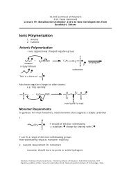
Infrasound<br />
3.1 Physical characteristics<br />
3<br />
In general, sound waves are longitudinal waves <strong>of</strong> which <strong>the</strong> particle or oscillator<br />
motion is in <strong>the</strong> same direction as <strong>the</strong> wave propagation. A sound wave traveling<br />
through a gas disturbs <strong>the</strong> equilibrium state <strong>of</strong> <strong>the</strong> gas by compressions and<br />
rarefactions. Sound waves are elastic waves, thus, when particles are displaced,<br />
a force proportional to <strong>the</strong> displacement acts on <strong>the</strong> particles to restore <strong>the</strong>m<br />
to <strong>the</strong>ir original position, see e.g. Pain [1983].<br />
Here, infrasonic waves in <strong>the</strong> <strong>atmosphere</strong> are considered in <strong>the</strong> frequency<br />
range <strong>of</strong> 0.002 to 20 Hz, which travel <strong>with</strong> <strong>the</strong> speed <strong>of</strong> sound and have amplitudes<br />
in <strong>the</strong> order <strong>of</strong> 10 −2 Pa to 10 2 Pa at <strong>the</strong> receiver, after having traveled<br />
for hundreds to thousands <strong>of</strong> kilometers.<br />
Figure 3.1: The frequency and periods <strong>of</strong> acoustic (sound) and non-acoustic waves<br />
(gravity waves).<br />
19
20 Infrasound<br />
Figure 3.2: Frequency ω versus wavenumber m plot from Gossard and Hooke [1975].<br />
NA is called <strong>the</strong> acoustic cut-<strong>of</strong>f frequency, N <strong>the</strong> Brunt-Väisälä frequency and Ωz<br />
represents <strong>the</strong> angular frequency <strong>of</strong> <strong>the</strong> earth’s rotation.<br />
3.1.1 Frequency contents<br />
A large range <strong>of</strong> frequencies <strong>of</strong> <strong>the</strong>se deformations can be facilitated by <strong>the</strong> gas.<br />
Sound waves in <strong>the</strong> <strong>atmosphere</strong> become audible to humans if <strong>the</strong> frequency is in<br />
<strong>the</strong> range <strong>of</strong> 20 to 20.000 Hz. Ultrasonic sound is inaudible to humans and has<br />
frequencies higher than 20.000 Hz. For example, bats use this high frequency<br />
sound as sonar for orientation purposes. At <strong>the</strong> o<strong>the</strong>r end <strong>of</strong> <strong>the</strong> spectrum,<br />
sound also becomes inaudible, when <strong>the</strong> frequency is lower than 20 Hz. Sound<br />
waves are <strong>the</strong>n called <strong>infrasound</strong>, equivalent to low frequency light which is<br />
called infrared and invisible (see Figure 3.1).<br />
The lower limit <strong>of</strong> <strong>infrasound</strong> is bounded by <strong>the</strong> thickness <strong>of</strong> <strong>the</strong> atmospheric<br />
layer through which it travels. When <strong>the</strong> wavelengths <strong>of</strong> <strong>infrasound</strong> become too<br />
long, gravity starts acting on <strong>the</strong> mass displacement. <strong>Acoustic</strong>-gravity and gravity<br />
waves are <strong>the</strong> results if gravity becomes part <strong>of</strong> <strong>the</strong> restoring force. <strong>Acoustic</strong>gravity<br />
and gravity (or buoyancy) waves are <strong>the</strong> result if gravity becomes part<br />
<strong>of</strong> <strong>the</strong> restoring force. Figure 3.2 schematically illustrates <strong>the</strong> domains <strong>of</strong> <strong>the</strong><br />
different wave types by means <strong>of</strong> disperion curves [Gossard and Hooke, 1975].<br />
The acoustic cut-<strong>of</strong>f frequency NA is typically 3.3 mHz and <strong>the</strong> Brunt-Väisälä<br />
frequency N is 2.9 mHz in <strong>the</strong> lower <strong>atmosphere</strong> (see also Figure 3.1).<br />
3.1.2 Propagation velocity<br />
Infrasound travels <strong>with</strong> <strong>the</strong> speed <strong>of</strong> sound, 343 m/s at 20 ◦ C in air near <strong>the</strong><br />
earth’s surface. This velocity will increase at higher temperatures and in a down<br />
wind situation and vice verse. Fur<strong>the</strong>rmore, this velocity depends on <strong>the</strong> type
3.2 Sources 21<br />
<strong>of</strong> gas, i.e. <strong>the</strong> fundamental property <strong>of</strong> <strong>the</strong> material, which also holds for solids<br />
and fluids. Low-frequency waves in <strong>the</strong> <strong>atmosphere</strong> <strong>with</strong> a velocity lower than<br />
<strong>the</strong> sound speed also occur, but <strong>the</strong> restoring force is gravity. Gravity waves<br />
typically travel <strong>with</strong> wind speed like velocities in <strong>the</strong> order <strong>of</strong> 1 to 10 m/s.<br />
Infrasound wave propagation is, in first order, dependent on <strong>the</strong> composition<br />
and wind and temperature structure <strong>of</strong> <strong>the</strong> <strong>atmosphere</strong>. The effective sound<br />
speed incorporates <strong>the</strong>se effects and described by e.g. Gossard and Hooke [1975]<br />
and Pierce [1989]:<br />
ceff = γgRcTa + ˆnxy · u (3.1.1)<br />
where <strong>the</strong> multiplication <strong>of</strong> <strong>the</strong> ratio <strong>of</strong> specific heats <strong>with</strong> <strong>the</strong> gas constant<br />
for air is γgRc=402.8 m 2 s −2 K −1 . The absolute temperature is given by Ta<br />
and ˆnxy · u projects <strong>the</strong> wind u in <strong>the</strong> direction from source to observer ˆnxy.<br />
The temperature decreases <strong>with</strong> altitude in <strong>the</strong> lower <strong>atmosphere</strong>, under regular<br />
atmospheric circumstances. As a result <strong>of</strong> this, sound bends upward as function<br />
<strong>of</strong> horizontal distance. Refraction <strong>of</strong> <strong>infrasound</strong> back to <strong>the</strong> surface may occur<br />
from regions where ceff becomes large than its surface value. This can be caused<br />
by an increase in wind or temperature or a combined effect. Refraction follows<br />
from Snell’s law and will bend <strong>infrasound</strong> back to <strong>the</strong> earth’s surface.<br />
3.1.3 Amplitude<br />
The pressure fluctuations <strong>of</strong> sound waves are, in general, small <strong>with</strong> respect<br />
to <strong>the</strong> ambient pressure. For example, an average sound volume setting <strong>of</strong> a<br />
television set in a living room, will result in pressure fluctuations <strong>of</strong> 0.02 Pa (60<br />
dB relative to 20 µPa) against a standard background pressure <strong>of</strong> 1013 hPa.<br />
Infrasound roughly deals <strong>with</strong> receiving amplitudes <strong>of</strong> hundredths to tens <strong>of</strong><br />
pascals. If <strong>the</strong> amplitude becomes too large, <strong>the</strong> linearity <strong>of</strong> <strong>the</strong> longitudinal<br />
acoustic wave is lost and shock waves occur. Shock waves are non-linear waves<br />
that propagate at velocities higher than <strong>the</strong> sound speed. As <strong>the</strong> energy <strong>of</strong> <strong>the</strong><br />
shock wave dissipates, a linear acoustic wave will remain if sufficient energy is<br />
available. Due to its low frequency content, <strong>infrasound</strong> can travel over enormous<br />
distance as it experiences little attenuation.<br />
3.2 Sources<br />
In general, <strong>infrasound</strong> is generated when a large volume <strong>of</strong> air is displaced.<br />
Sources <strong>of</strong> <strong>infrasound</strong> are, consequently, large and powerful.<br />
3.2.1 Anthropogenic<br />
• Airplanes:<br />
– Sub-sonic: regular air traffic generates <strong>infrasound</strong>. On a quiet night<br />
when <strong>the</strong> measurement conditions are ideal, air planes can be tracked<br />
when flying over or nearby an <strong>infrasound</strong> array at altitudes up to 10<br />
km to distances over 30 km [Evers, 2005].
22 Infrasound<br />
– Super-sonic: a shock wave is created when a plane travels close to<br />
<strong>the</strong> speed <strong>of</strong> sound. At short distances, this so-called sonic boom<br />
can be heard as two loud bangs being <strong>the</strong> front and back <strong>of</strong> <strong>the</strong><br />
plane flying through <strong>the</strong> sound barrier. At larger distances, <strong>the</strong> high<br />
frequency audible part is attenuated and <strong>infrasound</strong> travels fur<strong>the</strong>r<br />
over hundreds <strong>of</strong> kilometers. Infrasound from <strong>the</strong> Concorde has been<br />
used in an early stage to probe <strong>the</strong> upper <strong>atmosphere</strong> [Balachandran<br />
et al., 1977; Liszka, 1978].<br />
• Chemical explosions: large explosions like, for example, accidental chemical<br />
explosions generate <strong>infrasound</strong>. Infrasound from military test and<br />
natural sources was already used by Gutenberg [1939] to visualize <strong>the</strong><br />
stratosphere through a refractive sequence <strong>of</strong> zones <strong>of</strong> silence and strong<br />
infrasonic signals observed at <strong>the</strong> earth’s surface.<br />
• Gas flares: <strong>infrasound</strong> has been observed by Liszka [1974] from gas exhausts<br />
near oil fields on <strong>the</strong> North Sea. More recently, <strong>infrasound</strong> has<br />
been associated to <strong>the</strong> burning <strong>of</strong> gas near oil and gas fields in Kazakhstan<br />
[Smirnov, 2006].<br />
• Nuclear tests: atmospheric nuclear tests generate <strong>infrasound</strong> that can<br />
travel around <strong>the</strong> globe several times if <strong>the</strong> yield is large enough. This<br />
was <strong>the</strong> case <strong>with</strong> <strong>the</strong> megaton TNT tests on Novaya Zemlya in <strong>the</strong> 1960s.<br />
Also smaller test can be detected over large ranges [Posey and Pierce,<br />
1971].<br />
3.2.2 Natural<br />
• Aurora: <strong>the</strong> movement <strong>of</strong> large volumes <strong>of</strong> air in <strong>the</strong> upper <strong>atmosphere</strong> by<br />
aurora, leads to a notable infrasonic signal at <strong>the</strong> earth’s surface. These<br />
signals were first discovered in Alaska by Wilson [1967] and come in various<br />
types depending on <strong>the</strong> type <strong>of</strong> aurora, e.g. as shock waves or pulsating<br />
<strong>infrasound</strong>.<br />
• Avalanches: when large volumes <strong>of</strong> snow and ice are displaced, <strong>infrasound</strong><br />
is generated. Measurement systems in <strong>the</strong> Swiss Alps have been set up to<br />
monitor avalanches [Van Lancker, 2001].<br />
• Earthquakes: <strong>infrasound</strong> from earthquakes can be recorded in two ways.<br />
Firstly, upward traveling <strong>infrasound</strong> causes ionospheric disturbances [Blanc,<br />
1985] that can be measured by GPS systems [Calais and Minster, 1995].<br />
Secondly, <strong>infrasound</strong> can travel directly from <strong>the</strong> source region to <strong>the</strong> observer<br />
[Beni<strong>of</strong>f and Gutenberg, 1939]. In both cases, displacements <strong>of</strong> <strong>the</strong><br />
earth’s surface over large regions cause this <strong>infrasound</strong>.<br />
• Lightning: cloud-to-cloud and cloud-to-ground discharges cause <strong>infrasound</strong><br />
because a shock wave is generated by <strong>the</strong> <strong>the</strong>rmal expansion <strong>of</strong> <strong>the</strong> lightning<br />
channel [Few, 1969]. Huge mass displacements take place <strong>with</strong>in<br />
<strong>the</strong> clouds when charges are reorganized which also lead to <strong>infrasound</strong><br />
[Dessler, 1973]. Cloud-to-ground discharges in <strong>the</strong> Ne<strong>the</strong>rlands have been<br />
detected over ranges <strong>of</strong> 50 km and can be explained by a line-source model
3.2 Sources 23<br />
[Assink et al., 2008]. A more exotic type <strong>of</strong> <strong>infrasound</strong> is generated by transient<br />
luminous events such as sprites [Liszka, 2004; Farges et al., 2005].<br />
These are discharges from <strong>the</strong> top <strong>of</strong> <strong>the</strong> clouds upwards to <strong>the</strong> ionosphere.<br />
• Meteors: <strong>infrasound</strong> is generated when a meteoroid enters <strong>the</strong> <strong>atmosphere</strong><br />
at hyper-sonic speeds. Infrasound can also be caused by fragmentation <strong>of</strong><br />
<strong>the</strong> meteoroid. Most meteoroids end <strong>the</strong>ir journey <strong>with</strong> a <strong>the</strong>rmal explosion<br />
at 30 to 50 km altitude, generating additional <strong>infrasound</strong> [ReVelle,<br />
1976]. Infrasound from <strong>the</strong> Siberian Tunguska meteor was recorded in<br />
1908, June 30 on <strong>the</strong> first microbarometers [Shaw and Dines, 1904] in <strong>the</strong><br />
UK and analyzed by Whipple [1930].<br />
• Oceanic waves: <strong>the</strong> non-linear interaction <strong>of</strong> oceanic waves traveling in<br />
almost opposite directions generates microbaroms in <strong>the</strong> <strong>atmosphere</strong> and<br />
microseism in <strong>the</strong> solid earth. These waves coincide <strong>with</strong> large low pressure<br />
systems over <strong>the</strong> oceans, where strong winds act on <strong>the</strong> ocean surface.<br />
Microbaroms were first discovered by Beni<strong>of</strong>f and Gutenberg [1939] and<br />
later ma<strong>the</strong>matically described by Longuet-Higgins [1950].<br />
• Severe wea<strong>the</strong>r: large storms and storm cells contain turbulent structures<br />
on all scales including shear winds. These huge displacements generate<br />
<strong>infrasound</strong> signals that have been detected over ranges <strong>of</strong> more than 1000<br />
km [Bowman and Bedard, 1971].<br />
• Volcanoes: <strong>the</strong> first instrumentally recorded <strong>infrasound</strong> event was <strong>the</strong> explosion<br />
<strong>of</strong> <strong>the</strong> Krakatoa near Java in Indonesia on 1883, August 27. The<br />
<strong>infrasound</strong> was recorded on traditional barographs and traveled around<br />
<strong>the</strong> world four times [Symons, 1888].
24 Infrasound
The <strong>atmosphere</strong> as medium <strong>of</strong><br />
propagation<br />
4.1 Characteristics<br />
4<br />
Infrasound wave propagation is dependent on <strong>the</strong> wind and temperature structure<br />
and composition <strong>of</strong> <strong>the</strong> <strong>atmosphere</strong>. The <strong>atmosphere</strong> is a dynamic medium<br />
where changes occur on a wide range <strong>of</strong> spatial and temporal scales, influencing<br />
<strong>the</strong> propagation <strong>of</strong> <strong>infrasound</strong>.<br />
4.1.1 Temperature and wind<br />
The <strong>atmosphere</strong> is divided into several layers. Naming <strong>of</strong> <strong>the</strong>se layers can be<br />
based on, for example, how well mixed a certain portion <strong>of</strong> <strong>the</strong> <strong>atmosphere</strong> is.<br />
Turbulent eddies lead to a well mixed <strong>atmosphere</strong> below 100 km. Above 100 km,<br />
turbulent air motions are strongly damped and diffusion becomes <strong>the</strong> preferred<br />
mechanism for vertical transport. Above an altitude <strong>of</strong> 500 km, <strong>the</strong> critical level,<br />
molecular collisions are so rare that molecules leave <strong>the</strong> denser <strong>atmosphere</strong> into<br />
space if <strong>the</strong>ir velocity is high enough to escape <strong>the</strong> earth’s gravitational field.<br />
Based on <strong>the</strong> above, <strong>the</strong> first 100 km is called <strong>the</strong> homosphere. Split by <strong>the</strong><br />
homopause, <strong>the</strong> area ranging from 100 to 500 km is called <strong>the</strong> heterosphere.<br />
The region from 500 km upward is named <strong>the</strong> exosphere [Salby, 1996].<br />
Naming can also be based on <strong>the</strong> sign <strong>of</strong> temperature gradients in different<br />
parts <strong>of</strong> <strong>the</strong> <strong>atmosphere</strong>. This is more convenient for <strong>the</strong> study <strong>of</strong> <strong>infrasound</strong><br />
since <strong>the</strong> propagation <strong>of</strong> <strong>infrasound</strong> is partly controlled by temperature. The<br />
temperature distribution <strong>with</strong>in a standard <strong>atmosphere</strong> is given in Figure 4.1.<br />
The pr<strong>of</strong>ile shows a sequence <strong>of</strong> negative and positive temperature gradients<br />
which are separated by small regions <strong>of</strong> constant temperature. From bottom<br />
to top, <strong>the</strong> <strong>atmosphere</strong> is divided into layers called <strong>the</strong> troposphere, stratosphere,<br />
mesosphere and <strong>the</strong>rmosphere, <strong>the</strong>se are separated by <strong>the</strong> tropopause,<br />
stratopause and mesopause, respectively.<br />
25
26 The <strong>atmosphere</strong> as medium <strong>of</strong> propagation<br />
Altitude(km)<br />
140<br />
130<br />
120<br />
110<br />
100<br />
90<br />
80<br />
70<br />
60<br />
50<br />
40<br />
30<br />
20<br />
10<br />
0<br />
Homosphere Heterosphere<br />
Homo<br />
pause<br />
Mesopause<br />
Stratopause<br />
Tropopause<br />
Boundary layer<br />
-100 -50 0 50 100 150 200 250<br />
Temperature( o C)<br />
Thermosphere<br />
Mesosphere<br />
Stratosphere<br />
Troposphere<br />
Figure 4.1: The temperature in <strong>the</strong> <strong>atmosphere</strong> as function <strong>of</strong> altitude based on <strong>the</strong><br />
average kinetic energy <strong>of</strong> <strong>the</strong> atoms, from <strong>the</strong> U.S. Standard Atmosphere [NOAA et al.,<br />
1976].<br />
Altitude(km)<br />
120<br />
110<br />
100<br />
90<br />
80<br />
70<br />
60<br />
50<br />
40<br />
30<br />
20<br />
10<br />
0<br />
Winter<br />
Summer<br />
-100 0 100 200<br />
T( o C)<br />
-40 0 40 80<br />
Zw(m/s)<br />
to E<br />
-20 0 20 40 60<br />
Mw(m/s)<br />
Figure 4.2: NRL-G2S pr<strong>of</strong>iles for 2006, July 01 (in black) and December 01 (in gray)<br />
at 12 UTC in De Bilt, <strong>the</strong> Ne<strong>the</strong>rlands, at 52 ◦ N, 5 ◦ E [Drob et al., 2003].<br />
to N
4.1 Characteristics 27<br />
In <strong>the</strong> standard <strong>atmosphere</strong>, <strong>the</strong> temperature decreases <strong>with</strong> altitude in <strong>the</strong><br />
troposphere. In a real <strong>atmosphere</strong>, a temperature inversion may occur when<br />
<strong>the</strong> temperature increases <strong>with</strong> altitude in <strong>the</strong> first 100 m up to a couple <strong>of</strong> km.<br />
After a constant temperature in <strong>the</strong> tropopause, <strong>the</strong> temperature increases in<br />
<strong>the</strong> stratosphere due to <strong>the</strong> presence <strong>of</strong> ozone. The so-called ozone layer consists<br />
<strong>of</strong> this radiatively active trace gas and absorbs UV radiation. After a decrease<br />
in temperature in <strong>the</strong> mesosphere, <strong>the</strong> temperature rises again in <strong>the</strong> <strong>the</strong>rmosphere<br />
due to highly energetic solar radiation which is absorbed by very small<br />
residuals <strong>of</strong> molecular oxygen and nitrogen gases. The temperature around 300<br />
km altitude can vary from 700 to 1600 ◦ C depending on <strong>the</strong> solar activity.<br />
Figure 4.2 shows <strong>the</strong> temperature and wind pr<strong>of</strong>iles for summer and winter<br />
in De Bilt, <strong>the</strong> Ne<strong>the</strong>rlands, at 52 ◦ N, 5 ◦ E. The wind is split in a West-East<br />
component that is called <strong>the</strong> zonal wind and in a South-North component, <strong>the</strong><br />
meridional wind. The zonal wind is directed positive when blowing from <strong>the</strong><br />
West towards <strong>the</strong> East, a westerly wind. The meridional wind has a positive sign<br />
if it originates in <strong>the</strong> South. Two regions in <strong>the</strong> <strong>atmosphere</strong> are <strong>of</strong> importance<br />
for <strong>infrasound</strong> propagation, as far as wind is concerned. Firstly, <strong>the</strong> jet stream<br />
just below <strong>the</strong> tropopause, which is caused by temperature difference between<br />
<strong>the</strong> pole and equator in combination <strong>with</strong> <strong>the</strong> Coriolis force. The temperature<br />
gradient is much higher in winter than in summer. Therefore, <strong>the</strong> maximum<br />
zonal wind speed is largest in winter. The o<strong>the</strong>r is, <strong>the</strong> zonal mean circulation in<br />
<strong>the</strong> stratosphere. The main features, consistent <strong>with</strong> <strong>the</strong> temperature gradient<br />
from winter to summer pole, are an easterly jet in <strong>the</strong> summer hemisphere and<br />
a westerly one in winter. The maximum wind speeds <strong>of</strong> this polar vortex occur<br />
around an altitude <strong>of</strong> 60 km and are again largest in winter [Holton, 1979].<br />
In summary, wind and temperature conditions that strongly influence <strong>infrasound</strong><br />
propagation in <strong>the</strong> lower <strong>atmosphere</strong> are <strong>the</strong> occurrence <strong>of</strong> a temperature<br />
inversion in <strong>the</strong> troposphere and <strong>the</strong> existence <strong>of</strong> a jet stream near <strong>the</strong><br />
tropopause. For <strong>the</strong> middle <strong>atmosphere</strong>, important conditions are <strong>the</strong> strong<br />
temperature increase <strong>with</strong>in <strong>the</strong> stratospheric ozone layer and <strong>the</strong> polar vortex.<br />
Upper atmospheric propagation will be controlled by <strong>the</strong> positive temperature<br />
gradient in <strong>the</strong> <strong>the</strong>rmosphere.<br />
4.1.2 Composition<br />
The <strong>atmosphere</strong> is composed <strong>of</strong> 78% molecular nitrogen and 21% molecular<br />
oxygen. The remaining 1% consists <strong>of</strong> water vapor, carbon dioxide, ozone and<br />
o<strong>the</strong>r minor constituents (see Figure 4.3). The global mean pressure and density<br />
decrease approximately exponentially <strong>with</strong> altitude (see Figure 4.4). Pressure<br />
decreases from 10 5 Pa, at <strong>the</strong> surface, to 10% <strong>of</strong> that value at an altitude <strong>of</strong><br />
15 km. Consequently, 90% <strong>of</strong> <strong>the</strong> <strong>atmosphere</strong>’s mass is present in <strong>the</strong> first 15<br />
km altitude. The density decreases at <strong>the</strong> same rate from a surface value <strong>of</strong> 1.2<br />
kg/m 3 . The mean free path <strong>of</strong> molecules varies proportionally to <strong>the</strong> inverse <strong>of</strong><br />
density. Therefore, it increases exponentially <strong>with</strong> altitude from 10 −7 m at <strong>the</strong><br />
surface to 1 m at 100 km [Salby, 1996].
28 The <strong>atmosphere</strong> as medium <strong>of</strong> propagation<br />
Figure 4.3: The composition <strong>of</strong> <strong>the</strong> <strong>atmosphere</strong>, in terms <strong>of</strong> molar weight, as function<br />
<strong>of</strong> altitude, from <strong>the</strong> U.S. Standard Atmosphere [NOAA et al., 1976]. This figure is<br />
taken from Salby [1996].<br />
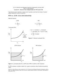
4.2 Refractions <strong>with</strong> raytracing<br />
Figure 4.5 shows an example <strong>of</strong> raytracing [Garcés et al., 1998] through <strong>the</strong><br />
summer situation presented in Figure 4.2. Rays are shot from <strong>the</strong> source at a<br />
distance and altitude <strong>of</strong> 0 km, each four degrees from <strong>the</strong> vertical to <strong>the</strong> horizontal.<br />
Both westward and eastward atmospheric trajectories are given which are<br />
controlled by <strong>the</strong> effective velocity structure, see Equation 3.1.1. The effective<br />
velocity pr<strong>of</strong>ile for westward propagation is given in <strong>the</strong> left frame <strong>of</strong> Figure<br />
4.5, <strong>the</strong> eastward effective velocity is given in <strong>the</strong> right-hand frame. Infrasound<br />
refracts back to <strong>the</strong> surface from regions where ceff increases to a value larger<br />
than <strong>the</strong> value at <strong>the</strong> surface. This surface value <strong>of</strong> ceff is given by <strong>the</strong> dashed<br />
vertical line in <strong>the</strong> left and right-hand frames <strong>of</strong> Figure 4.5. The polar vortex is<br />
directed from East to West. Therefore, stratospheric refractions are predicted<br />
for energy traveling to <strong>the</strong> West. The corresponding arrivals are labeled as Is,<br />
Is2 indicates that two refractions have occurred. Some <strong>the</strong>rmospheric paths<br />
(It) are also present to <strong>the</strong> West. The counteracting polar vortex results in<br />
solely <strong>the</strong>rmospheric arrivals towards <strong>the</strong> East.<br />
Where Figure 4.5 only represents an West-East cross section, Figure 4.6<br />
shows <strong>the</strong> bounce points <strong>of</strong> <strong>the</strong> rays on <strong>the</strong> earth’s surface in all directions. The<br />
source is located in <strong>the</strong> center <strong>of</strong> <strong>the</strong> figure. Stratospheric arrivals (in blue)<br />
are refracted from altitudes <strong>of</strong> 45 to 55 km, while <strong>the</strong>rmospheric arrivals (in<br />
darkblue) result from refractions <strong>of</strong> altitudes between 100 and 125 km. This<br />
image is only valid for 2006, July 01 at 12 UTC for a ceff at 52 ◦ N, 5 ◦ E and
4.3 Absorption 29<br />
Figure 4.4: The pressure and density in <strong>the</strong> <strong>atmosphere</strong> as function <strong>of</strong> altitude, from<br />
<strong>the</strong> U.S. Standard Atmosphere [NOAA et al., 1976]. This figure is taken from Salby<br />
[1996].<br />
will change as function <strong>of</strong> time and geographical position. Therefore, Figure 4.6<br />
also illustrates <strong>the</strong> challenge in understanding <strong>the</strong> atmospheric propagation <strong>of</strong><br />
<strong>infrasound</strong>. In winter time, <strong>the</strong> above picture, for <strong>the</strong> summer time, reverses as<br />
<strong>the</strong> stratospheric winds have changed direction towards <strong>the</strong> East. There is also<br />
a thin troposheric duct present for energy traveling towards <strong>the</strong> East. Phases<br />
trapped in such a surface duct are labeled Iw and are more visible in Figure 4.7<br />
in light blue.<br />
4.3 Absorption<br />
The absorption <strong>of</strong> sound in <strong>the</strong> <strong>atmosphere</strong> is a function <strong>of</strong> frequency and decreases<br />
<strong>with</strong> decreasing frequency. The absorption in a molecular gas is caused<br />
by two different mechanisms, which are <strong>the</strong> classical and relaxation effects. The<br />
classical effects are formed by transport processes in a gas. These are molecular<br />
diffusion, internal friction and heat conduction. The latter two have <strong>the</strong> largest<br />
contribution. The relaxation effects follow from <strong>the</strong> compressional energy which<br />
is stored in <strong>the</strong> internal degrees <strong>of</strong> freedom <strong>of</strong> <strong>the</strong> molecules. It requires time<br />
to (de)excitate internal energy states which occur during collisions. The relax-
30 The <strong>atmosphere</strong> as medium <strong>of</strong> propagation<br />
Altitude(km)<br />
120<br />
110<br />
100<br />
90<br />
80<br />
70<br />
60<br />
50<br />
40<br />
30<br />
20<br />
10<br />
0<br />
0.3 0.4<br />
c eff(km/s)<br />
West<br />
-600 -400 -200 0 200 400 600<br />
Distance(km)<br />
East<br />
Is2 Is<br />
It It2<br />
0.3 0.4<br />
c eff(km/s)<br />
Figure 4.5: Raytracing for a source at a distance and altitude <strong>of</strong> 0 km. Rays are<br />
shot each four degrees from <strong>the</strong> vertical to <strong>the</strong> horizontal in a westward and eastward<br />
direction through <strong>the</strong> summer situation as given in Figure 4.2. Effective speeds are<br />
given in <strong>the</strong> left and right frame, <strong>the</strong> dashed vertical line represents <strong>the</strong> effective speed<br />
at <strong>the</strong> surface.<br />
ation effects can be split in a vibrational and rotational component. Both <strong>the</strong><br />
classical and relaxation effects are a function <strong>of</strong> frequency to <strong>the</strong> power <strong>of</strong> two<br />
[Bass et al., 1972].<br />
Figure 4.8 shows an example <strong>of</strong> <strong>the</strong> adsorption <strong>of</strong> <strong>infrasound</strong> by using <strong>the</strong><br />
results from Bass et al. [1972]. This figure is taken from Le Pichon et al. [2008]<br />
and uses <strong>the</strong> NRL-RAMPE parabolic equation method [Lingevitch et al., 2002]<br />
combined <strong>with</strong> <strong>the</strong> environmental pr<strong>of</strong>iles derived from <strong>the</strong> G2S atmospheric<br />
model [Drob et al., 2003]. These are compared to a 3D ray traces adapted from<br />
<strong>the</strong> Tau-P method [Garcés et al., 1998]. Since effects <strong>of</strong> <strong>the</strong> boundary conditions<br />
<strong>of</strong> <strong>the</strong> propagation domain are particularly important in <strong>the</strong> high-altitude Andes<br />
region, simulations account for <strong>the</strong> NOAA Global Land One-km Base Elevation<br />
(GLOBE) digital terrain elevation model [Hastings and Dunbar, 1998].
4.3 Absorption 31<br />
Figure 4.6: Raytracing through <strong>the</strong> summer <strong>atmosphere</strong> from Figure 4.2 in all directions.<br />
The source is located in <strong>the</strong> center. The bounce points <strong>of</strong> <strong>the</strong> rays on <strong>the</strong> earth’s<br />
surface are shown as function <strong>of</strong> distance, up to 600 km, and propagation direction.<br />
The North is located at zero degrees and <strong>the</strong> East at 90 degrees. The arrivals are labeled<br />
using <strong>the</strong> same convention as Figure 4.5, where a West (270 degrees) to East (90<br />
degrees) cross section was shown. Blue colors refer to stratospheric phases (Is) and<br />
dark blue is used for rays impinging on <strong>the</strong> earth’s surface after being refracted and<br />
having turned in <strong>the</strong> <strong>the</strong>rmosphere (It phases).
32 The <strong>atmosphere</strong> as medium <strong>of</strong> propagation<br />
Figure 4.7: Raytracing through <strong>the</strong> winter pr<strong>of</strong>iles in all directions up to a distance <strong>of</strong><br />
600 km. The bounce points <strong>of</strong> <strong>the</strong> rays on <strong>the</strong> earth’s are plotted for a source located in<br />
<strong>the</strong> center at an altitude <strong>of</strong> 0 km. Light blue color refer to tropospheric phases (Iw),<br />
blue for stratospheric phases (Is) and dark blue for <strong>the</strong>rmospheric arrivals (It).
4.3 Absorption 33<br />
Figure 4.8: The loss <strong>of</strong> energy in dB (colour coded) for different source altitudes (A,<br />
B, C, D: 10, 25, 35 and 50 km, respectively) for a 1 Hz wave. The source is a meteor<br />
over Bolivia [Le Pichon et al., 2008]. The propagation <strong>of</strong> <strong>infrasound</strong> waves is modeled<br />
towards <strong>the</strong> souteast in <strong>the</strong> direction <strong>of</strong> I41PY (an IMS <strong>infrasound</strong> array in Paraguay).<br />
The topography represents <strong>the</strong> Andes.
34 The <strong>atmosphere</strong> as medium <strong>of</strong> propagation
Measurement <strong>of</strong> <strong>infrasound</strong> data<br />
5.1 The KNMI microbarometer<br />
5<br />
Various instruments have been developed which have <strong>the</strong> ability to detect <strong>infrasound</strong>,<br />
like: differential [Cook and Bedard, 1971] and absolute microbarometers<br />
[Grover, 1971], vector sensors [Evers et al., 2000; van Zon et al., 2009], loudspeakers<br />
[Beni<strong>of</strong>f and Gutenberg, 1939], piezo-electrical [De Wolf , 2006] and<br />
fiber-optical devices [Zumberge et al., 2003]. This section describes <strong>the</strong> constructional<br />
efforts for a differential microbarometer which is capable <strong>of</strong> measuring<br />
<strong>infrasound</strong> in <strong>the</strong> range <strong>of</strong> 500 seconds up to 20 Hz. Not only acoustic waves<br />
and events <strong>of</strong> CTBT interest occur in this pass-band but also gravity waves,<br />
i.e, internal waves <strong>with</strong> gravity as restoring force [Gossard and Hooke, 1975]. A<br />
differential microbarometer was chosen because it has several advantages when<br />
compared to o<strong>the</strong>r instruments. Those are its simple configuration, low price<br />
reproducibility, tunable response and durability.<br />
5.1.1 Design and construction<br />
The infrasonic frequency range <strong>of</strong> interest is 0.002 to 20 Hz and can be measured<br />
by ei<strong>the</strong>r making a microphone low frequency or a barometer high frequency.<br />
Microphones tend to be sensitive to moisture and will, <strong>the</strong>refore, degrade during<br />
<strong>the</strong> required continuous operation. Fur<strong>the</strong>rmore, <strong>the</strong> response <strong>of</strong> most commercially<br />
available microphones will severely drop at frequencies lower than 10 Hz.<br />
As an alternative, low frequency loudspeakers, wo<strong>of</strong>ers, can be used to measure<br />
<strong>infrasound</strong> if mounted in a box. But <strong>the</strong>se also suffer from <strong>the</strong> lack <strong>of</strong> durability<br />
in outdoor operations and sensitivity at very low frequencies. Consequently,<br />
it was chosen to adapt a barometer to higher frequencies and make it more<br />
sensitive to small air pressure fluctuations. A barometer typically measures air<br />
pressure fluctuations in <strong>the</strong> order <strong>of</strong> 100 hPa and samples <strong>the</strong> <strong>atmosphere</strong> every<br />
1 to 10 seconds. In <strong>the</strong> <strong>infrasound</strong> application <strong>the</strong> measurement device should<br />
be capable <strong>of</strong> resolving fluctuations in <strong>the</strong> order <strong>of</strong> 10 −2 Pa and sample at at<br />
least 40 Hz.<br />
35
36 Measurement <strong>of</strong> <strong>infrasound</strong> data<br />
COIL<br />
E−CORE<br />
DIAPHRAGM<br />
CAPILLARY<br />
BACKING<br />
VOLUME<br />
ELECTRONICS BOX<br />
INLET BOX<br />
VALIDYNE SENSOR<br />
Figure 5.1: Schematic overview <strong>of</strong> <strong>the</strong> KNMI microbarometer. The <strong>atmosphere</strong> is sampled<br />
through <strong>the</strong> inlet box where pressure fluctuations are measured by <strong>the</strong> Validyne<br />
sensor. A backing volume is attached to <strong>the</strong> sensor to construct a differential instrument.<br />
Within <strong>the</strong> backing volume, an acoustical resistance, i.e. capillary, is mounted<br />
to ”leak” very low frequency pressure fluctuations back to <strong>the</strong> <strong>atmosphere</strong>. Various<br />
elements <strong>of</strong> <strong>the</strong> Validyne sensor are shown in <strong>the</strong> inlay being <strong>the</strong> e-cores, coils and<br />
diaphragm.<br />
Figure 5.1 shows a schematic overview <strong>of</strong> <strong>the</strong> microbarometer developed by <strong>the</strong><br />
KNMI. The <strong>atmosphere</strong> is sampled through <strong>the</strong> inlet box to which a commercial<br />
pressure sensor is attached. Validyne Eng. fabricates pressure sensors sensitive<br />
to very low fluctuations. These so-called ultra, or very low range, differential<br />
pressure transducers come in various sensitivities. Within <strong>the</strong> microbarometer,<br />
type DP-103 (ultra low, 0.022 to 0.35 kPa at ± 10 Vdc Full Scale) and DP-45<br />
(very low, 0.14 to 0.35 kPa FS) are deployed. The natural frequency <strong>of</strong> <strong>the</strong><br />
sensor is 600 Hz which is far above <strong>the</strong> upper limit <strong>of</strong> <strong>the</strong> frequency range <strong>of</strong><br />
interest. The inset in Figure 5.1 shows <strong>the</strong> details <strong>of</strong> <strong>the</strong> pressure sensor. The<br />
pressure <strong>sensing</strong> diaphragm is mounted between coils and free to move in response<br />
to differential pressure. The coils are matched and wired in series in an<br />
inductive half-bridge. The coils are fed <strong>with</strong> an AC excitation to create a magnetic<br />
flux. Movement <strong>of</strong> <strong>the</strong> diaphragm will lead to a change in coil impedance<br />
which, in turn, will bring <strong>the</strong> half-bridge out <strong>of</strong> balance. An AC signal will<br />
appear directly proportional to <strong>the</strong> applied pressure. The phase <strong>of</strong> <strong>the</strong> signal<br />
is determined by <strong>the</strong> direction <strong>of</strong> movement <strong>of</strong> <strong>the</strong> diaphragm. The coils are<br />
enclosed <strong>with</strong>in two e-like shaped cores to close <strong>the</strong> magnetic circuit.<br />
A backing volume is attached to <strong>the</strong> pressure sensor. Thus, a differential microbarometer<br />
has been created capable <strong>of</strong> measuring over <strong>the</strong> whole frequency<br />
range <strong>of</strong> atmospheric pressure fluctuations, also those <strong>of</strong> meteorological origin.
5.1 The KNMI microbarometer 37<br />
r<br />
R<br />
CAPILLARY<br />
P +P<br />
A e<br />
b<br />
DIAPHRAGM<br />
INLETS AND<br />
NOISE REDUCER<br />
V P +P<br />
A<br />
v P +p<br />
A<br />
FORE VOLUME<br />
BACKING VOLUME<br />
Figure 5.2: Schematic drawing <strong>of</strong> <strong>the</strong> microbarometer adapted after Burridge [1971].<br />
Two volumes V and v are connected by a high acoustic resistance r. The <strong>atmosphere</strong><br />
is sampled through <strong>the</strong> noise reducers and inlets that have a low acoustic resistance<br />
R. An external pressure Pe is applied to <strong>the</strong> system. The observed pressure difference<br />
∆Pobs = P − p, <strong>with</strong> respect to <strong>the</strong> ambient pressure PA, is sensed by <strong>the</strong> diaphragm<br />
that undergoes a volume change b as function <strong>of</strong> this pressure.<br />
A low frequency cut-<strong>of</strong>f is realized by including a leak in <strong>the</strong> backing volume.<br />
This leak consists <strong>of</strong> a thin capillary that acts as acoustic resistance, redirecting<br />
fluctuations <strong>with</strong> too long periods back to <strong>the</strong> <strong>atmosphere</strong>. The length and<br />
diameter <strong>of</strong> <strong>the</strong> capillary and <strong>the</strong> size <strong>of</strong> <strong>the</strong> backing volume determine <strong>the</strong> low<br />
frequency cut-<strong>of</strong>f.<br />
Additional electronics are needed to supply <strong>the</strong> sensor <strong>with</strong> power and to read<br />
and transmit <strong>the</strong> out-coming signal. This electronics board is mounted in a<br />
separate box below <strong>the</strong> sensor. In a later version <strong>of</strong> <strong>the</strong> microbarometer, <strong>the</strong><br />
electronics are included in <strong>the</strong> same box as <strong>the</strong> sensor.<br />
5.1.2 Theoretical microbarometer response<br />
Burridge [1971] derived <strong>the</strong> <strong>the</strong>oretical response for a microbarograph. Figure<br />
5.2 shows <strong>the</strong> different elements <strong>of</strong> <strong>the</strong> microbarometer. The fore volume <strong>of</strong><br />
size V is connected to <strong>the</strong> <strong>atmosphere</strong> which has an ambient pressure PA. The<br />
<strong>atmosphere</strong> is sampled through <strong>the</strong> inlets and an additional analog noise reducer<br />
<strong>with</strong> a low acoustical resistance R. A backing volume is present <strong>of</strong> size v. A<br />
pressure difference between <strong>the</strong> two chambers is sensed by <strong>the</strong> diaphragm <strong>of</strong><br />
<strong>the</strong> Validyne sensor. In <strong>the</strong> work <strong>of</strong> Burridge [1971], pressure-sensitive bellows<br />
were used to sense <strong>the</strong> pressure difference. The volume change as function <strong>of</strong><br />
pressure <strong>with</strong>in <strong>the</strong> Validyne sensor is denoted by b. The backing volume is<br />
connected to <strong>the</strong> fore volume by a high acoustic resistance r, i.e. <strong>the</strong> capillary.<br />
An external pressure <strong>of</strong> size Pe results in an observed pressure difference <strong>of</strong><br />
∆Pobs = P −p between <strong>the</strong> fore and backing volume. The phase and amplitude<br />
<strong>of</strong> this difference are detected by <strong>the</strong> diaphragm.
38 Measurement <strong>of</strong> <strong>infrasound</strong> data<br />
The air initially occupying <strong>the</strong> fore and back volume is perturbed by <strong>the</strong> external<br />
pressure Pe. By evaluating Boyle’s law, differentiated <strong>with</strong> respect to time,<br />
Burridge [1971] derived <strong>the</strong> <strong>the</strong>oretical microbarometer response as function <strong>of</strong><br />
frequency ω, as:<br />
where<br />
D = ∆Pobs<br />
Pe<br />
A = 1<br />
PA<br />
=<br />
PA<br />
α = 1<br />
PA<br />
<br />
1<br />
+ b<br />
V<br />
<br />
iω<br />
β + iωα + iωRV<br />
PA<br />
+ b 1<br />
, β =<br />
v rv<br />
1<br />
<br />
+ , B =<br />
v<br />
1<br />
<br />
1<br />
r V<br />
(5.1.1)<br />
(B + iωA)<br />
1<br />
<br />
+<br />
v<br />
(5.1.2)<br />
(5.1.3)<br />
The described response has a lower and upper frequency limit. At low frequencies,<br />
large volumes and high acoustic resistances will control <strong>the</strong> behaviour <strong>of</strong><br />
<strong>the</strong> instrument. The small volumes and low acoustic resistances will dominate<br />
at high frequencies. Equation 5.1.1 can be rewritten as:<br />
D =<br />
1<br />
PAβ<br />
iω + PAα RV B iωARV<br />
+ + PA PA<br />
(5.1.4)<br />
The first and last term in <strong>the</strong> denominator <strong>of</strong> equation 5.1.4 contain frequency<br />
ω; <strong>the</strong> middle two terms are constants. At low frequencies, <strong>the</strong> first term will<br />
dominate. Thus, <strong>the</strong> response in <strong>the</strong> low frequency limit is:<br />
D ∼ iωrv<br />
PA<br />
The second term is important at high frequencies, leading to:<br />
1<br />
D ∼ <br />
1 iωRV + b PA<br />
<br />
1<br />
V<br />
(5.1.5)<br />
(5.1.6)<br />
1 + v<br />
As expected, <strong>the</strong> low frequency response is controlled by <strong>the</strong> large backing volume<br />
v and <strong>the</strong> capillary as high acoustic resistance r. The small fore volume<br />
V and inlets, <strong>with</strong> a low acoustic resistance R, determine <strong>the</strong> high frequency<br />
response.<br />
5.1.3 The low frequency cut-<strong>of</strong>f<br />
Theoretical derivation<br />
The low frequency cut-<strong>of</strong>f fl <strong>of</strong> <strong>the</strong> KNMI microbarometer is controlled by <strong>the</strong><br />
characteristics <strong>of</strong> <strong>the</strong> capillary and <strong>the</strong> size <strong>of</strong> <strong>the</strong> backing volume. The acoustical<br />
resistance <strong>of</strong> <strong>the</strong> capillary r is described by:<br />
r = P<br />
dv/dt<br />
(5.1.7)<br />
<strong>with</strong>, P as pressure and dv/dt represents a volume change <strong>with</strong> time. Equation<br />
5.1.7 is equivalent to Ohm’s law for <strong>the</strong> electrical resistance R as function <strong>of</strong>
5.1 The KNMI microbarometer 39<br />
voltage V and current I, being R = V/I. Poiseuille’s law couples <strong>the</strong> resistance<br />
<strong>of</strong> a flow through <strong>the</strong> capillary to its length l and radius a, by:<br />
r = 8lη<br />
πa 4<br />
(5.1.8)<br />
where <strong>the</strong> viscosity η equals 18.27 µPa s at 18◦C. Equation 5.1.8 is valid for<br />
small pressure fluctuations <strong>with</strong> respect to <strong>the</strong> background pressure, which is<br />
generally true for acoustics waves in <strong>the</strong> <strong>atmosphere</strong>. The capillary is characterized<br />
by a=0.1 mm and l=10 cm, resulting in a r <strong>of</strong> 4.65x10¹⁰ kg m−4s−1 .<br />
The low-frequency cut-<strong>of</strong>f fl <strong>of</strong> a system can be written, by using <strong>of</strong> <strong>the</strong> relaxation<br />
time τ, as:<br />
fl = 1<br />
(5.1.9)<br />
2πτ<br />
The corresponding value is known as <strong>the</strong> −3 dB point or <strong>the</strong> level at which<br />
<strong>the</strong> amplitude has decreased <strong>with</strong> e−1 . In electronics, τ = RC is known as<br />
<strong>the</strong> RC-time <strong>of</strong> a circuit which contains a resistance R and a capacitance C.<br />
Equivalently, equation 5.1.9 is used to determine <strong>the</strong> frequency cut-<strong>of</strong>f <strong>of</strong>, for<br />
example, an analog filter.<br />
From equation 5.1.5 and 5.1.9 it follows that:<br />
fl ∼ PA<br />
2πrv<br />
(5.1.10)<br />
This equation also shows <strong>the</strong> analogy <strong>of</strong> <strong>the</strong> acoustic resistance r and electrical<br />
resistance R and that <strong>of</strong> a volume v and capacitance C. The low frequency<br />
cut-<strong>of</strong>f <strong>of</strong> <strong>the</strong> microbarometer is <strong>the</strong>oretically determined <strong>with</strong> equation 5.1.10,<br />
as fl ∼3.5x10 −3 Hz <strong>with</strong> v=100 ml and PA=1.01325x10 5 Pa.<br />
Experimental determination<br />
The low frequency cut-<strong>of</strong>f can also be determined experimentally as described<br />
by Evers and Haak [2000]. In essence, <strong>the</strong> relaxation time <strong>of</strong> <strong>the</strong> instrument<br />
is measured after a sudden over- or under-pressure, i.e. <strong>the</strong> impulse response.<br />
The relaxation <strong>of</strong> <strong>the</strong> diaphragm is described by Haak and de Wilde [1996] and<br />
follows <strong>the</strong> relation:<br />
Pt<br />
P0<br />
= Vt<br />
V0<br />
= e −αt<br />
(5.1.11)<br />
where, P0 represents <strong>the</strong> over-pressured starting situation which is relaxed in<br />
time t. Within <strong>the</strong> sensor, pressure variations, Pt, are directly proportional to<br />
voltage variations Vt. The capillary controls <strong>the</strong> time necessary to reach an<br />
equilibrium, between <strong>the</strong> open air and backing volume, by a constant α. The<br />
relaxation time τ is defined as <strong>the</strong> time necessary to let <strong>the</strong> amplitude decay to<br />
e −1 , <strong>the</strong> −3 dB point, from which it follows that:<br />
e −αt = e −1 → α = 2πfl = 1<br />
τ<br />
(5.1.12)<br />
Figure 5.3 shows <strong>the</strong> results <strong>of</strong> <strong>the</strong> relaxation experiment obtained after suddenly<br />
opening one <strong>of</strong> <strong>the</strong> inlets <strong>of</strong> <strong>the</strong> microbarometer. It follows from this experiment<br />
and that <strong>the</strong> low frequency cut-<strong>of</strong>f equals: 1.85±0.01x10 −3 Hz. This value was
40 Measurement <strong>of</strong> <strong>infrasound</strong> data<br />
Voltage (V)<br />
9<br />
8<br />
7<br />
6<br />
5<br />
4<br />
3<br />
2<br />
1<br />
0<br />
V o<br />
V o e-1<br />
V o e-2<br />
t o τ 2 τ<br />
0 30 60 90 120 150 180 210 240 270 300 330 360 390<br />
Time (s)<br />
Figure 5.3: Response <strong>of</strong> <strong>the</strong> microbarometer to a sudden under-pressure. The relaxation<br />
time, τ, can be derived at various levels, n, <strong>of</strong> V0e −nτ .<br />
Table 5.1: Sizes <strong>of</strong> <strong>the</strong> microbarometer’s components, acoustical resistances and volume<br />
change<br />
size<br />
length capillary 10x10 −2 m<br />
diameter capillary 0.1x10 −3 m<br />
r: resistance 4.65x10 10 kg m −4 s −1<br />
length inlet 6x10 −2 m<br />
diameter inlet 10x10 −3 m<br />
R: resistance 279 kg m −4 s −1<br />
volumetric displacement pressure cavity 4.9x10 −8 m 3<br />
at DP-103 Full Scale 0.35x10 3 Pa<br />
b: volume change 1.4x10 −10 m 3 Pa −1<br />
v: backing volume 100x10 −6 m 3<br />
V : fore volume 22.1x10 −6 m 3<br />
again obtained <strong>with</strong> a capillary <strong>of</strong> 0.1 mm radius and length <strong>of</strong> 10 cm, <strong>with</strong>in<br />
a backing volume <strong>of</strong> 100 ml. The period <strong>of</strong> <strong>the</strong> instrument can be increased by<br />
increasing <strong>the</strong> acoustical resistance <strong>of</strong> <strong>the</strong> capillary by, for example, increasing<br />
its length or decreasing <strong>the</strong> diameter.<br />
The <strong>the</strong>oretically and experimentally derived low frequency cut-<strong>of</strong>f differ because<br />
<strong>of</strong> <strong>the</strong> strong dependence on <strong>the</strong> diameter a <strong>of</strong> <strong>the</strong> capillary. In equation 5.1.8,<br />
a is present to <strong>the</strong> fourth power. Therefore, small variations in <strong>the</strong> diameter <strong>of</strong><br />
0.1 mm will have a large influence on <strong>the</strong> low frequency cut-<strong>of</strong>f.
5.1 The KNMI microbarometer 41<br />
Amplitude<br />
Phase(rad)<br />
2<br />
1<br />
0<br />
-1<br />
-2<br />
10 0<br />
10 -1<br />
10 -2<br />
-3 dB<br />
10 -4 10 -3 10 -2 10 -1 10 0 10 1 10 2 10 3 10 4 10 5 10 6 10 7 10 8 10 9<br />
Angular frequency(rad/s)<br />
Figure 5.4: The amplitude and phase response <strong>of</strong> <strong>the</strong> KNMI microbarometer as function<br />
<strong>of</strong> <strong>the</strong> angular frequency ω. The black line represents <strong>the</strong> <strong>the</strong>oretical response based on<br />
equation 5.1.1. The gray line is <strong>the</strong> true response experimentally determined for <strong>the</strong><br />
low frequency cut-<strong>of</strong>f. The −3dB points are given by <strong>the</strong> intersections <strong>of</strong> <strong>the</strong> dashed<br />
line.<br />
5.1.4 Response <strong>of</strong> <strong>the</strong> KNMI microbarometer<br />
The amplitude and phase response <strong>of</strong> <strong>the</strong> microbarometer are given in Figure<br />
5.4. The sizes <strong>of</strong> different components, as input for this calculation, are listed in<br />
Table 5.1. In this table, values are derived for <strong>the</strong> acoustical resistances r and<br />
R, and volume change b. The amplitude is calculated by taking <strong>the</strong> absolute<br />
value <strong>of</strong> D (equation 5.1.1); <strong>the</strong> phase follows from <strong>the</strong> argument <strong>of</strong> D. The<br />
black line is <strong>the</strong> <strong>the</strong>oretical response. The gray line represents <strong>the</strong> true response<br />
which was experimentally determined for <strong>the</strong> low frequency cut-<strong>of</strong>f.<br />
The <strong>the</strong>oretical response is flat up to a high value <strong>of</strong> <strong>the</strong> angular frequency ω.<br />
The high frequency cut-<strong>of</strong>f <strong>of</strong> 9.2x10 6 rad/s, or 1.5x10 6 Hz, is far above <strong>the</strong><br />
infrasonic upper frequency limit <strong>of</strong> 20 Hz. However, this <strong>the</strong>oretical value will<br />
not be reached in practice, because:<br />
• A noise reducer will be attached to <strong>the</strong> system to sample <strong>the</strong> <strong>atmosphere</strong><br />
(see Section 5.1.5), and will act as a low-pass filter at higher frequencies.<br />
Typically, this filter will attenuate frequencies higher than 50 Hz,<br />
depending on <strong>the</strong> size <strong>of</strong> <strong>the</strong> noise reducer.<br />
• The natural frequency <strong>of</strong> <strong>the</strong> Validyne sensor is 600 Hz, which leads to
42 Measurement <strong>of</strong> <strong>infrasound</strong> data<br />
5 m<br />
75 cm<br />
80 cm<br />
PVC CONTAINER<br />
INSULATION<br />
CLOSED<br />
HOSE<br />
KNMI MICROBAROMETER<br />
ELECTRONICS BOX<br />
50 cm<br />
CONCRETE PROTECTION<br />
POWER CABLE<br />
SIGNAL CABLE<br />
POROUS HOSE<br />
SURFACE<br />
Figure 5.5: Typical installation <strong>of</strong> <strong>the</strong> KNMI microbarometer as element <strong>of</strong> an <strong>infrasound</strong><br />
array. The microbarometer is installed in a watertight PVC tube beneath <strong>the</strong><br />
surface. Next to its subsurface mounting, Styr<strong>of</strong>oam plates are placed <strong>with</strong>in <strong>the</strong> tube<br />
to ensure temperature stability. Porous hoses and cables are tightly connected through<br />
cable swivels. Additional protection is obtained by a concrete cover also serving as<br />
supplemental insulation device.<br />
resonances at and around this frequency. Fur<strong>the</strong>rmore, a Helmholtz resonator<br />
has been created by combining an inlet and fore volume. This<br />
resonance is around 400 Hz, using <strong>the</strong> geometric values given in Table 5.1.<br />
From <strong>the</strong> phase response, it becomes clear that <strong>the</strong> microbarometer differentiates<br />
signals <strong>with</strong> a very low frequency content. This will lead to a 90 degrees,<br />
or π<br />
2 , phase shift <strong>of</strong> <strong>the</strong> recorded signals. Therefore, signals recorded at <strong>the</strong>se<br />
very low frequencies should be corrected for <strong>the</strong> instrument’s response. This<br />
correction can be approximated by integrating <strong>the</strong> signal [Christie et al., 1978].<br />
The sensitivity <strong>of</strong> <strong>the</strong> microbarometer was determined by a simple calibration<br />
experiment [Evers and Haak, 2000]. The microbarometer was vertically displaced<br />
over a certain distance h. The induced pressure variation ∆P and vertical<br />
distance are related through:<br />
∆P = ρgh (5.1.13)<br />
<strong>with</strong> <strong>the</strong> density <strong>of</strong> air ρ and gravitational acceleration g. The instrument was<br />
displaced over known distances multiple times, which resulted in an average<br />
value for <strong>the</strong> sensitivity <strong>of</strong> 5.65x10 −2 Pa/mV.<br />
More details on <strong>the</strong> microbarometer response will become available in Mentink<br />
and Evers [2008].<br />
5.1.5 Field installation<br />
The microbarometer is installed below <strong>the</strong> earth’s surface in a watertight PVC<br />
tube (Figure 5.5). Subsurface mounting is important to ensure temperature
5.1 The KNMI microbarometer 43<br />
Figure 5.6: Installation <strong>of</strong> a microbarometer in DIA. The microbarometer is installed<br />
beneath <strong>the</strong> earth’s surface and covered by a concrete top. The <strong>atmosphere</strong> is sampled<br />
by six porous hoses in a star-like layout, each <strong>of</strong> 5 m length.<br />
INTERNET<br />
230 VAC<br />
LINUX PC<br />
ROUTER<br />
NETWORK CARD<br />
GPS CLOCK CARD<br />
ADC CARD<br />
EXTERNAL USB<br />
BACKUP DISK<br />
GPS<br />
ANTENNA<br />
SIGNAL<br />
INSIDE CENTRAL<br />
FACILITY<br />
27 VDC<br />
MICRO−<br />
CABLE BOX BAROMETER<br />
27 VDC<br />
AC/DC CONVERTER<br />
230V/27V<br />
SIGNAL<br />
NOISE<br />
REDUCER<br />
OUTSIDE<br />
Figure 5.7: Architecture <strong>of</strong> a typical <strong>infrasound</strong> measurement system. The various<br />
components both in- and outside <strong>the</strong> central facility are shown.
44 Measurement <strong>of</strong> <strong>infrasound</strong> data<br />
stability. The microbarometer is a differential pressure sensor and, <strong>the</strong>refore,<br />
sensitive to temperature fluctuations. Mainly temperature fluctuations <strong>with</strong> periods<br />
smaller than 500 s will affect <strong>the</strong> pressure in <strong>the</strong> backing volume and lead<br />
to a notable signal <strong>with</strong>in <strong>the</strong> frequency range <strong>of</strong> interest. Fur<strong>the</strong>r insulation is<br />
achieved by placing Styr<strong>of</strong>oam plates in <strong>the</strong> tube and <strong>the</strong> placement <strong>of</strong> a concrete<br />
cover which also serves as protection. Temperature measurements inside<br />
<strong>the</strong> PVC tube have shown no correlation between <strong>the</strong> measured temperature<br />
and pressure fluctuations for periods less than at least 1000 s [Mentink and<br />
Evers, 2008]. A power and signal cable are connected to <strong>the</strong> microbarometer<br />
through cable swivels.<br />
The measurement <strong>of</strong> <strong>infrasound</strong> is affected by noise from wind. Typically, between<br />
1 and 10 Hz winds will affect <strong>the</strong> <strong>infrasound</strong> signals <strong>of</strong> interest. Therefore,<br />
analog filters are applied that use <strong>the</strong> large coherency length <strong>of</strong> <strong>infrasound</strong> versus<br />
<strong>the</strong> short coherency length <strong>of</strong> wind to improve <strong>the</strong> signal-to-noise ratio <strong>of</strong><br />
<strong>the</strong> recording. By sampling <strong>the</strong> <strong>atmosphere</strong> over an area ra<strong>the</strong>r than at one<br />
point, incoherent wind is canceled out while <strong>the</strong> infrasonic signal remains unaffected.<br />
Figure 5.6 shows an analog filter constructed <strong>with</strong> six porous or soaker<br />
hoses <strong>of</strong> 5 m length in a star-like configuration. Impermeable hoses <strong>of</strong> 1.5 m<br />
are used close to <strong>the</strong> instrument, to avoid sampling <strong>of</strong> a possible coherent wind<br />
field. O<strong>the</strong>r such filters can consist <strong>of</strong> pipes [Daniels, 1950] and [Daniels, 1959]<br />
or pipe arrays <strong>with</strong> discrete inlets [Hedlin et al., 2003]. Wind barriers are also<br />
applied and can be constructed <strong>of</strong> wood [Liszka, 2008] or porous shade cloth<br />
[Christie, 2007]. The spatial design <strong>of</strong> noise reducers depends on <strong>the</strong> infrasonic<br />
freqeuncy range <strong>of</strong> interest and <strong>the</strong> expected wind speeds [Wilson et al., 2007].<br />
The spatial coherence <strong>of</strong> <strong>the</strong> wind field increases <strong>with</strong> increasing wind speeds<br />
but remains only a small fraction <strong>the</strong> coherence <strong>of</strong> <strong>the</strong> infrasonic wave [Shields,<br />
2005].<br />
Both signal and power cables originate from a central facility where 27 VDC/2<br />
A is provided as power to <strong>the</strong> microbarometers. Here, <strong>the</strong> analog signals are<br />
also collected. The analog signals are converted to digital by a National Instrument’s<br />
16 bits analog-digital converter (ADC) board mounted in a Linux<br />
driven PC. The board is accessed through free driver s<strong>of</strong>tware made available<br />
at www.comedi.org and incorporated in a data acquisition program. The signals<br />
are accurately time stamped, i.e. at sub-sample rate values, by a GPS<br />
clock provided by Meinberg Funkuhren GmbH & Co., that is also accessible under<br />
Linux. The data can be accessed, all year round (24/7), through TCP/IP<br />
protocols like secure shell (ssh) and <strong>the</strong> file transfer protocol (ftp) or pushed<br />
from a <strong>remote</strong> site to <strong>the</strong> user over <strong>the</strong> Internet. All components <strong>of</strong> <strong>the</strong> <strong>infrasound</strong><br />
measurement system, both in- and outside, are summarized in Figure 5.7.<br />
5.2 Arrays for <strong>infrasound</strong> measurements<br />
Infrasound is measured <strong>with</strong> arrays <strong>of</strong> microbarometers. These arrays reduce<br />
noise through signal summation, ideally leading to 1/ √ N increase in signalto-noise<br />
ratio, in case <strong>of</strong> uncorrelated noise, where N is <strong>the</strong> number <strong>of</strong> array<br />
elements. Fur<strong>the</strong>rmore, array processing techniques enable <strong>the</strong> characterization<br />
<strong>of</strong> <strong>the</strong> signal in terms <strong>of</strong> back azimuth and apparent sound speed. In <strong>the</strong> first
5.2 Arrays for <strong>infrasound</strong> measurements 45<br />
section, <strong>the</strong> array response will be derived, which forms <strong>the</strong> basis for array<br />
design. For this purpose, beamforming and <strong>the</strong> frequency-wavenumber spectral<br />
density will be introduced. These will also be applied later in array processing.<br />
5.2.1 Beamforming array response pattern<br />
An <strong>infrasound</strong> array consists <strong>of</strong> N microbarometers in a limited aperture. The<br />
reconstruction <strong>of</strong> <strong>the</strong> wavefield is affected by this spatial discretization since <strong>the</strong><br />
<strong>atmosphere</strong> is not sampled infinitely.<br />
Assume we have a monochromatic three-dimensional wavefield <strong>of</strong> unit amplitude<br />
described by:<br />
g(t,r) = e i(2πf0t−k0·r) (5.2.14)<br />
<strong>with</strong> frequency f0, traveltime t, wavenumber k0 = (k0x, k0y, k0z) at position<br />
r = (x, y, z).<br />
The Fourier transform <strong>of</strong> this signal is given by:<br />
being<br />
G(f,r) =<br />
∞<br />
−∞<br />
G(f,r) = δ(f − f0)e −i k0·r<br />
g(t,r)e −i2πft dt (5.2.15)<br />
(5.2.16)<br />
A wavefield can be characterized by means <strong>of</strong> a spectral density function. This is<br />
a frequency-wavenumber (f/k) spectral density function for propagating waves,<br />
or a homogeneous random field. Such a f/k spectral density function provides<br />
information on <strong>the</strong> process as a function <strong>of</strong> frequency and <strong>the</strong> vector velocities<br />
<strong>of</strong> propagating waves [Capon, 1969]. The f/k density function for <strong>the</strong> assumed<br />
planar wavefield, is defined as (see e.g. [Denholm-Price and Rees, 1999]):<br />
G(f; kx, ky) =<br />
∞ ∞<br />
G(f,r)e<br />
−∞ −∞<br />
i(k·r) dxdy (5.2.17)<br />
<strong>with</strong>: k = (kx, ky) and <strong>the</strong> positions r = (rx, ry) located at z = 0, i.e. <strong>the</strong><br />
earth’s surface.<br />
By using <strong>the</strong> result <strong>of</strong> <strong>the</strong> Fourier transform (5.2.16), <strong>the</strong> f/k spectral function<br />
becomes:<br />
G(f, k) = δ(f − f0)δ(kx − k0x)δ(ky − k0y) (5.2.18)<br />
The maximum value <strong>of</strong> G(f, k) is found at (f0, k0).<br />
Arrays <strong>of</strong> microbarometers discretely sample <strong>the</strong> wavefield above <strong>the</strong> array in<br />
two dimensions. Spatial sampling is controlled by N sensors located at positions<br />
rj = (xj, yj), while <strong>the</strong> sample rate ∆ determines <strong>the</strong> temporal sampling. The<br />
discrete form <strong>of</strong> <strong>the</strong> frequency-wavenumber power spectrum <strong>of</strong> <strong>the</strong> acquired data<br />
is defined [Smart and Flinn, 1971]:<br />
P(ω, k) =<br />
N<br />
N<br />
j=1 m=1<br />
w(rj)w(rm)Sjm(ω)e i k·(rj−rm)<br />
(5.2.19)<br />
where P(ω, k) represents an estimate for <strong>the</strong> f/k power spectrum, Sjm(ω) is<br />
<strong>the</strong> cross-spectrum between <strong>the</strong> jth and mth sensor as function <strong>of</strong> ω, which is
46 Measurement <strong>of</strong> <strong>infrasound</strong> data<br />
<strong>the</strong> angular frequency and equals 2πf. If it is assumed that all instruments are<br />
equally sensitive to <strong>the</strong> plane wave than w(rj) = w(rm)=1.<br />
The Fourier transform G(f,r) (equation 5.2.15) can be written as Aj(ω)e iϕj(ω)<br />
which contains <strong>the</strong> amplitude and phase information <strong>of</strong> <strong>the</strong> signal in <strong>the</strong> frequency<br />
domain for <strong>the</strong> jth sensor. The cross-spectrum between <strong>the</strong> jth and<br />
mth sensor can <strong>the</strong>n be written as:<br />
Sjm(ω) = Aj(ω)e −iϕj(ω) · Am(ω)e iϕm(ω)<br />
(5.2.20)<br />
which follows from <strong>the</strong> correlation <strong>the</strong>orem for real signals h1(t) and h2(t),<br />
generally stated as:<br />
C(h1, h2) ⇐⇒ H1(f)H ∗ 2 (f) = H1(f)H2(−f) (5.2.21)<br />
where H∗ 2 (f) is <strong>the</strong> complex conjugate <strong>of</strong> H2(f).<br />
It follows from <strong>the</strong> substitution <strong>of</strong> equation 5.2.20 in 5.2.19 that:<br />
By using:<br />
P(ω, k) =<br />
N<br />
j=1<br />
P(ω, k) =<br />
Aj(ω)e −i[ϕj(ω)− k·rj]<br />
N<br />
c<br />
j=1<br />
∗ j<br />
m=1<br />
N<br />
m=1<br />
Am(ω)e i[ϕm(ω)− k·rm]<br />
N<br />
cm = C ∗ C = |C| 2 <br />
N <br />
= <br />
<br />
n=1<br />
<strong>the</strong> double summation can than be rewritten as a single summation:<br />
P(ω, <br />
N<br />
<br />
k) = <br />
<br />
n=1<br />
G(ω,rn)e −i k·rn<br />
<br />
<br />
<br />
<br />
<br />
2<br />
cn<br />
<br />
<br />
<br />
<br />
<br />
2<br />
(5.2.22)<br />
(5.2.23)<br />
(5.2.24)<br />
The result found in equation 5.2.16 is now used to find <strong>the</strong> estimate for G(ω, k), being:<br />
P(ω, k) = [δ(ω − ω0)] 2<br />
<br />
N <br />
e<br />
<br />
−i(k− 2<br />
<br />
k0)·rn <br />
<br />
<br />
(5.2.25)<br />
Ideally, <strong>the</strong> best estimate for G(ω, k) is found for <strong>the</strong> limit <strong>of</strong> N → ∞:<br />
n=1<br />
∞<br />
e −i(k− k0)·rn → δ( k − k0) (5.2.26)<br />
n=1<br />
which means that <strong>the</strong> <strong>atmosphere</strong> is regularly sampled <strong>with</strong> an infinitely long<br />
array. With this result, we define <strong>the</strong> array response as:<br />
<strong>with</strong>:<br />
<br />
<br />
1<br />
R(ω, p) = <br />
N<br />
N<br />
n=1<br />
e −iω[(p−p0)·rn]<br />
<br />
<br />
<br />
<br />
<br />
2<br />
(5.2.27)<br />
p0 = 1<br />
ω (k0x, k0y) (5.2.28)
5.2 Arrays for <strong>infrasound</strong> measurements 47<br />
x<br />
x<br />
φ<br />
North<br />
wavefront<br />
1<br />
3<br />
n xy<br />
2<br />
z<br />
y<br />
φ<br />
wavefront<br />
1<br />
North<br />
n xy<br />
z<br />
3<br />
θ<br />
2<br />
C app<br />
C eff n<br />
,<br />
wavefront<br />
θ<br />
3 1 2<br />
C<br />
app<br />
C eff n<br />
,<br />
Figure 5.8: An inclined wavefront traveling over an array <strong>of</strong> three microbarometers<br />
located on <strong>the</strong> earth’s surface, i.e. xy-plane. The projection <strong>of</strong> <strong>the</strong> wavefront normal<br />
ˆn on <strong>the</strong> xy-plane is indicated by ˆnxy. The back azimuth φ is <strong>the</strong> clockwise angle<br />
between <strong>the</strong> propagation direction <strong>of</strong> <strong>the</strong> wave in <strong>the</strong> xy-plane, represented by <strong>the</strong> vector<br />
ˆnxy, and <strong>the</strong> North. The effective sound speed ceff is <strong>the</strong> velocity <strong>with</strong> which <strong>the</strong><br />
wave propagates through <strong>the</strong> air, i.e. in <strong>the</strong> xyz-space, and is directed normal ˆn to<br />
wavefront. The apparent sound speed capp is <strong>the</strong> velocity <strong>of</strong> <strong>the</strong> wavefront as measured<br />
by <strong>the</strong> microbarometers in <strong>the</strong> xy-plane. The apparent and effective sound speed are<br />
related through <strong>the</strong> inclination θ <strong>with</strong> capp ≥ ceff.<br />
y<br />
y
48 Measurement <strong>of</strong> <strong>infrasound</strong> data<br />
R(ω, p) is called <strong>the</strong> beamforming array response pattern [Capon, 1969], or<br />
spatial window function [Lacoss et al., 1969] or array transfer function [Denholm-<br />
Price and Rees, 1999].<br />
Beamforming is performed in <strong>the</strong> two-dimensional slowness (p = k ω ) domain to<br />
resolve <strong>the</strong> apparent sound speed capp and back azimuth φ, through:<br />
|p| = 1<br />
capp<br />
(5.2.29)<br />
px = |p| cosφ (5.2.30)<br />
py = |p| sin φ (5.2.31)<br />
Figure 5.8 shows an inclined wavefront in three spatial dimensions (x,y,z) traveling<br />
over a three element planar array, located at <strong>the</strong> earth’s surface, i.e. <strong>the</strong><br />
xy-plane. The back azimuth φ is <strong>the</strong> angle between <strong>the</strong> propagation direction<br />
<strong>of</strong> <strong>the</strong> wave in <strong>the</strong> xy-plane, given by <strong>the</strong> vector ˆnxy, and <strong>the</strong> North. The back<br />
azimuth is measured clockwise and gives <strong>the</strong> direction where <strong>the</strong> wave originates<br />
<strong>with</strong> respect to <strong>the</strong> receiver. In <strong>the</strong> example <strong>of</strong> Figure 5.8, φ equals 300◦ , which<br />
means a source located to <strong>the</strong> northwest <strong>of</strong> <strong>the</strong> array.<br />
The effective sound speed ceff, see equation 3.1.1, takes into account both <strong>the</strong><br />
effect <strong>of</strong> temperature and wind on <strong>the</strong> velocity <strong>of</strong> an infrasonic wave. Therefore,<br />
<strong>the</strong> effective sound speed is <strong>the</strong> propagation velocity <strong>of</strong> <strong>the</strong> inclined wavefront<br />
in <strong>the</strong> xyz-space, see Figure 5.8. The microbarometers measure a velocity in<br />
<strong>the</strong> xy-plane which is called <strong>the</strong> apparent sound speed capp. The apparent and<br />
effective sound speed are related through <strong>the</strong> inclination θ, as capp = ceff<br />
cos θ .<br />
There are two extreme cases in beamforming, as follow from equations 5.2.29<br />
through 5.2.31:<br />
• p = 0, capp = ∞ and θ = 90 ◦ : all instruments measure <strong>the</strong> waveform<br />
at <strong>the</strong> same time. This infinite capp means that <strong>the</strong>re are no traveltime<br />
differences over <strong>the</strong> array. The source will be located right above <strong>the</strong> array<br />
in <strong>the</strong> case <strong>of</strong> a planar wave.<br />
• capp = ceff and θ = 0 ◦ : <strong>the</strong> wavefront travels parallel (ˆn is in <strong>the</strong> same<br />
direction as ˆnxy) to <strong>the</strong> earth’s surface, or to <strong>the</strong> xy-plane in which <strong>the</strong><br />
instruments are located. The capp equals ceff which is also <strong>the</strong> lowermost<br />
possible value for capp. Only, for non-acoustic waves, like gravity waves,<br />
can capp be become smaller than ceff.<br />
5.2.2 Array design<br />
The temporal resolution is controlled by <strong>the</strong> sampling rate ∆, leading to a<br />
Nyquist frequency <strong>of</strong> fN = 1/2∆ which is <strong>the</strong> highest recoverable frequency<br />
given this digitization in time. Frequencies higher than fN will be aliased.<br />
Typical sample frequencies in <strong>infrasound</strong> measurements are in <strong>the</strong> order <strong>of</strong> 1 to<br />
200 Hz, depending on <strong>the</strong> frequency range <strong>of</strong> interest.<br />
Similarly, <strong>the</strong> resolution <strong>of</strong> an array is determined by <strong>the</strong> configuration and<br />
also limited by aliasing. A source cannot uniquely be identified if this so-called<br />
spatial aliasing occurs. In such a case, multiple solutions will exist for <strong>the</strong>
5.2 Arrays for <strong>infrasound</strong> measurements 49<br />
Figure 5.9: The columns show array layouts and <strong>the</strong>ir response patterns for simple three<br />
and four element configurations. A vertical incident planar wave, i.e. capp = ∞ and<br />
θ = 90 ◦ , peaks in <strong>the</strong> center <strong>of</strong> <strong>the</strong> graph. The top frame displays <strong>the</strong> array layout for<br />
array apertures <strong>of</strong> 1500 m. The amount <strong>of</strong> distances and angles between <strong>the</strong> elements<br />
are given in <strong>the</strong> next frames. In <strong>the</strong> lower four frames, <strong>the</strong> array responses are plotted<br />
for 0.15 and 0.4 Hz. The cross sections are also given at py = 0. The black circles<br />
in <strong>the</strong> response patterns represent an apparent sound speed <strong>of</strong> 340 m/s (on <strong>the</strong> black<br />
circle capp = ceff and θ = 0 ◦ ) defining <strong>the</strong> slowness interval <strong>of</strong> interest for <strong>infrasound</strong>.
50 Measurement <strong>of</strong> <strong>infrasound</strong> data<br />
apparent sound speed and back azimuth. In practice, <strong>the</strong> sensors <strong>with</strong>in an array<br />
are placed such that R(ω, p) in equation 5.2.27 approximates a delta function<br />
around <strong>the</strong> desired slowness p0 [Lacoss et al., 1969]. This discretization in space<br />
is realized by varying three parameters to design an optimal array, <strong>the</strong> diameter<br />
or aperture <strong>of</strong> <strong>the</strong> array, <strong>the</strong> number <strong>of</strong> sensors and <strong>the</strong> inter-sensor distances<br />
[Haubrich, 1968]. The lowest frequency that can be resolved by <strong>the</strong> array is<br />
determined by its aperture. The number <strong>of</strong> sensors and inter-sensor distances<br />
control <strong>the</strong> amount <strong>of</strong> spatial aliasing.<br />
The simplest and most effective three element planar array is realized when <strong>the</strong><br />
sensors are placed at <strong>the</strong> corners <strong>of</strong> an equilateral triangle. The left column <strong>of</strong><br />
Figure 5.9 shows <strong>the</strong> layout and array response patterns for 0.15 and 0.4 Hz.<br />
Also given are <strong>the</strong> number <strong>of</strong> inter-sensor distances, one in this case, and <strong>the</strong><br />
number <strong>of</strong> angles present between <strong>the</strong> elements. The distance between a pair <strong>of</strong><br />
sensors is is calculated by (∆x 2 +∆y 2 ). The angle between a pair <strong>of</strong> sensors is<br />
calculated by taking <strong>the</strong> absolute value <strong>of</strong> tangent <strong>of</strong> ∆y and ∆x. Both distance<br />
and angle are plotted for all possible sensor pairs in <strong>the</strong> second row from <strong>the</strong> top<br />
<strong>of</strong> Figure 5.9. As <strong>the</strong> aperture <strong>of</strong> <strong>the</strong> array and frequency range <strong>of</strong> operation<br />
scale linearly, this figure is valid for <strong>the</strong> whole range <strong>of</strong> acoustic frequencies.<br />
The black circle in response patterns represents a capp <strong>of</strong> 340 m/s. The cross<br />
section right above <strong>the</strong> pattern shows <strong>the</strong> response at py = 0. The main lobe <strong>of</strong><br />
<strong>the</strong> response, at px = py = 0, has a circular shape. This means that <strong>the</strong> array<br />
has no preferred orientations and will be equally sensitive in all directions. Side<br />
lobes are present near <strong>the</strong> main lobe and both are <strong>of</strong> equal size which will lead<br />
to spatial aliasing. This effect is clearly visible when <strong>the</strong> frequency is increased<br />
from 0.15 to 0.4 Hz and numerous lobes <strong>of</strong> unit amplitude are present in <strong>the</strong><br />
slowness domain <strong>of</strong> interest, making it impossible to identify <strong>the</strong> main lobe.<br />
If <strong>the</strong> number <strong>of</strong> sensors is increased from three to four, it seems logical to put<br />
<strong>the</strong>m equidistantly on a circle. The middle column <strong>of</strong> Figure 5.9 shows <strong>the</strong><br />
capabilities <strong>of</strong> such a circular array. The side lobes have moved somewhat away<br />
from <strong>the</strong> main lobe due to <strong>the</strong> increase in <strong>the</strong> number <strong>of</strong> inter-station distances<br />
and angles. This array will perform better over a wider range <strong>of</strong> frequencies<br />
than <strong>the</strong> triangular one. Although a circular array may seem appropriate, a<br />
more effective array can be constructed from four elements being a triangle<br />
<strong>with</strong> a central element. The right column in Figure 5.9 shows <strong>the</strong> layout and<br />
responses for this array. Nearby side lobes only have 50% <strong>of</strong> <strong>the</strong> amplitude<br />
<strong>of</strong> <strong>the</strong> main lobe. Spatial aliasing is avoided almost up to 0.4 Hz when <strong>the</strong><br />
first unit amplitude side lobes come in <strong>the</strong> slowness range <strong>of</strong> interest. The<br />
effect <strong>of</strong> increasing <strong>the</strong> number <strong>of</strong> inter-station distances and angles is hereby<br />
illustrated. The accuracy <strong>of</strong> <strong>the</strong> parameter estimation <strong>of</strong> <strong>infrasound</strong> arrays can<br />
be quantified by evaluating <strong>the</strong> distributions <strong>of</strong> <strong>the</strong> slowness estimates, which<br />
are event-specific [Szuberla and Olson, 2004].<br />
To summarize <strong>the</strong> above, <strong>the</strong> number <strong>of</strong> inter-station distances plays a decisive<br />
role in reaching an optimal array in <strong>the</strong> Fraunh<strong>of</strong>er approximation. These should<br />
allow for a wide range <strong>of</strong> distances, i.e. small and large, and various angles. The<br />
largest distance <strong>with</strong>in <strong>the</strong> array determines <strong>the</strong> lowest frequency that can be<br />
resolved. Therefore, <strong>the</strong> general design criteria are:<br />
• The main lobe has a circular shape. This means that <strong>the</strong> array is equally<br />
sensitive to all infrasonic arrivals, independent <strong>of</strong> its back azimuth.
5.2 Arrays for <strong>infrasound</strong> measurements 51<br />
• The main lobe is as small (”peaked”) as possible. The inclination and<br />
back azimuth will be resolved <strong>with</strong> <strong>the</strong> maximum accuracy since energy is<br />
minimally smeared out.<br />
• Side lobes are small in amplitude. Most energy is present in <strong>the</strong> main<br />
lobe, enabling maximum resolution and avoiding spatial aliasing.<br />
• Side lobes are as far away from <strong>the</strong> main lobe as possible. The main lobe<br />
will be unambiguously identified and spatial aliasing will be avoided.<br />
5.2.3 Infrasound arrays in <strong>the</strong> Ne<strong>the</strong>rlands<br />
Several arrays <strong>of</strong> microbarometers have been or are operational in <strong>the</strong> Ne<strong>the</strong>rlands.<br />
Figure 5.10 shows five <strong>infrasound</strong> arrays <strong>with</strong> various layouts and number<br />
<strong>of</strong> elements. The response patterns <strong>of</strong> <strong>the</strong> arrays are given in Figure 5.11 and<br />
are calculated for a monochromatic plane wave <strong>of</strong> 2 Hz. Clearly, <strong>the</strong> wide variety<br />
<strong>of</strong> number <strong>of</strong> instruments and array apertures gives different patterns. In<br />
general, <strong>the</strong> smaller <strong>the</strong> array, <strong>the</strong> broader its main lobe. The two extremes<br />
are DIA <strong>with</strong> an aperture <strong>of</strong> 1500 m and WIT <strong>with</strong> only 35 m. Where DIA<br />
starts approaching <strong>the</strong> desired delta function at 2 Hz, WIT is totally incapable<br />
<strong>of</strong> direction finding. All arrays are designed such that <strong>the</strong>y have a circular main<br />
lobe, guaranteeing unbiased omni-directional operation characteristics.
52 Measurement <strong>of</strong> <strong>infrasound</strong> data<br />
Figure 5.10: The locations <strong>of</strong> <strong>the</strong> <strong>infrasound</strong> arrays in <strong>the</strong> Ne<strong>the</strong>rlands. The array<br />
layouts are given in separate inlays.
5.2 Arrays for <strong>infrasound</strong> measurements 53<br />
Figure 5.11: Array responses <strong>of</strong> <strong>the</strong> <strong>infrasound</strong> arrays to a planar wave <strong>of</strong> 2 Hz. The<br />
wide variety <strong>of</strong> number <strong>of</strong> array elements and apertures causes different response patterns.
54 Measurement <strong>of</strong> <strong>infrasound</strong> data
Infrasound data processing<br />
6.1 General concept <strong>of</strong> <strong>infrasound</strong> data processing<br />
6<br />
Array processing is based on <strong>the</strong> detection <strong>of</strong> coherent signals and subsequent<br />
estimation <strong>of</strong> specific parameters to characterize <strong>the</strong> event. Infrasonic signals<br />
are continuously acquired at a rate <strong>of</strong> 40 samples per second and a detection<br />
algorithm is applied to find possible events <strong>of</strong> interest. Such detectors can<br />
perform in <strong>the</strong> time domain in search <strong>of</strong> correlated signals. Two correlation<br />
detectors are commonly used in <strong>infrasound</strong> data processing, being <strong>the</strong> Fisher<br />
detector [Melton and Bailey, 1957] and <strong>the</strong> Progressive Multi Channel Correlation<br />
technique, PMCC [Cansi, 1995]. Signal detection can also be achieved<br />
in <strong>the</strong> frequency domain, where signal coherency is used to trigger a detection<br />
[Smart and Flinn, 1971]. A comparison between <strong>the</strong> Fisher detector and <strong>the</strong><br />
PMCC technique has been made by Caljé [2005]. It was concluded that <strong>the</strong><br />
lower threshold for Fisher detection corresponds to a signal-to-noise power ratio<br />
<strong>of</strong> 0.05, which appeared to be 0.2 for <strong>the</strong> PMCC method.<br />
The Fisher detector analyzes variances <strong>with</strong>in measurements and is based on<br />
<strong>the</strong> work described by Fisher [1948]. Melton and Bailey [1957] introduced <strong>the</strong><br />
F-ratio which has been used in seismological studies by Blandford [1974] and<br />
more recently by Heyburn and Bowers [2007]. Based on experiences from seismology,<br />
Fisher detection has been proposed for <strong>the</strong> processing <strong>of</strong> <strong>infrasound</strong><br />
data by Brown et al. [2002] and has successfully detected sources like meteors<br />
and oceanic waves [Evers and Haak, 2001b].<br />
As introduced in Chapter 5, beamforming is applied to sample <strong>the</strong> <strong>atmosphere</strong><br />
above <strong>the</strong> array in all directions <strong>of</strong> interest. Parameters are estimated for a<br />
specific beam when a certain detection threshold is reached, i.e. an event is detected.<br />
The primary parameters are apparent sound speed and back azimuth.<br />
O<strong>the</strong>r event-specific parameters are frequency contents, amplitude and signalto-noise<br />
ratio.<br />
The following steps give an overview <strong>of</strong> <strong>the</strong> processing sequence:<br />
• Read <strong>the</strong> raw data. A filter can be applied before reading to concentrate<br />
55
56 Infrasound data processing<br />
on a specific frequency range, for example, a second order Butterworth<br />
band-pass filter. Any DC <strong>of</strong>fset or linear trend should be removed from<br />
<strong>the</strong> data because <strong>the</strong> Fourier transform would than be dominated by lowfrequency<br />
components.<br />
• Split <strong>the</strong> data in overlapping time segments, i.e. bins, if long time series are<br />
to be evaluated. In real-time processing, data are split in 50% overlapping<br />
bins <strong>with</strong> <strong>the</strong> length being at least <strong>the</strong> traveltime <strong>of</strong> a wave over <strong>the</strong> array.<br />
Doing so, it is ensured that a coherent wave, traveling over <strong>the</strong> array, is<br />
included in <strong>the</strong> bin.<br />
• Define a slowness p, see equations 5.2.29 through 5.2.31, interval <strong>of</strong> interest.<br />
Typically, a grid <strong>of</strong> 50x50 points is defined in <strong>the</strong> slowness range <strong>of</strong><br />
−0.005 to 0.005 s/m. The apparent velocity on such a grid varies between<br />
sub-acoustic velocities and infinity, which covers <strong>the</strong> apparent acoustic<br />
velocities.<br />
• Perform beamforming for each pair <strong>of</strong> (px, py) and run a detector on each<br />
beam. All 2500 time or phase differences are evaluated. These 2500 operations<br />
should be multiplied by <strong>the</strong> number <strong>of</strong> frequencies in <strong>the</strong> case <strong>of</strong><br />
a frequency domain detector. The one that explains <strong>the</strong> time or phase<br />
differences in <strong>the</strong> data best will lead to <strong>the</strong> highest detector value. The<br />
slowness, or apparent sound speed and back azimuth, for this beam will<br />
be stored, after which <strong>the</strong> next time segment can be evaluated.<br />
• Construct a best beam. The sum <strong>of</strong> all time aligned traces for <strong>the</strong> slowness<br />
at <strong>the</strong> maximum detector value is called <strong>the</strong> best beam. This can ei<strong>the</strong>r<br />
be done for each bin or for <strong>the</strong> maximum detector value from a set <strong>of</strong><br />
bins. Incoherent noise will cancel out and <strong>the</strong> signal will, consequently, be<br />
enhanced. The apparent sound speed and back azimuth are known at <strong>the</strong><br />
maximum detector value. The events are characterized.<br />
6.2 Time domain Fisher analysis<br />
The Fisher detector was first described by Melton and Bailey [1957] and aims to<br />
detect a coherent signal traveling over an array <strong>of</strong> sensors. This work was based<br />
on <strong>the</strong> analysis <strong>of</strong> variances [Fisher, 1948] <strong>of</strong> both noise and signal that are<br />
present in <strong>the</strong> recordings. Blandford [1974] successfully applied <strong>the</strong> F-detector<br />
to seismic array data, as was later done by Heyburn and Bowers [2007]. Applying<br />
a F-detector is attractive because <strong>of</strong> its well-known statistical distribution.<br />
In this section <strong>the</strong> approach <strong>of</strong> Melton and Bailey [1957] and Olson [2004] will<br />
be followed to derive <strong>the</strong> F-ratio, where in essence a statistical hypo<strong>the</strong>sis is<br />
tested.<br />
A statistical test is a set <strong>of</strong> rules whereby a decision about a hypo<strong>the</strong>sis is<br />
reached. The null hypo<strong>the</strong>sis that is being tested is designated H0. An alternative<br />
hypo<strong>the</strong>sis H1 will be accepted when H0 is rejected. The decision rules in<br />
<strong>the</strong> test are <strong>with</strong> respect to <strong>the</strong> rejection or non-rejection <strong>of</strong> H0. If <strong>the</strong> decision<br />
rules reject H0 when in fact H0 is true, <strong>the</strong> rules lead to an incorrect decision,<br />
called false alarm. The probability <strong>of</strong> making this so-called type 1 error is controlled<br />
by <strong>the</strong> chosen level <strong>of</strong> significance or threshold. A type 2 error is made
6.2 Time domain Fisher analysis 57<br />
Table 6.1: Statistical test and <strong>the</strong> errors, adapted after Winer [1962]. H represents a<br />
hypo<strong>the</strong>sis, E(F) <strong>the</strong> expected value <strong>of</strong> <strong>the</strong> Fisher ratio and σ 2 α a variance.<br />
H0 true H0 false<br />
H1 true<br />
Reject H0 Type 1 error No error<br />
False alarm<br />
Do not reject H0 No error Type 2 error<br />
Missed event<br />
σ 2 α = 0, E(F) = 1 σ 2 α > 0, E(F) > 1<br />
when <strong>the</strong> rules do not reject H0 when in fact H1 is true [Winer, 1962].<br />
The hypo<strong>the</strong>sis to be tested H0 is that all recordings made by <strong>the</strong> microbarometers<br />
consist <strong>of</strong> uncorrelated noise. The alternative hypo<strong>the</strong>sis H1 is valid<br />
for <strong>the</strong> case that not only noise is present but also signal. Evaluated are <strong>the</strong><br />
variance <strong>of</strong> <strong>the</strong> noise σ 2 and <strong>the</strong> variance σ 2 α, which can not be attributed to<br />
<strong>the</strong> noise since it is common to all signals. Table 6.1 summarizes <strong>the</strong> effects <strong>of</strong><br />
<strong>the</strong> decisions made in <strong>the</strong> statistical test based on <strong>the</strong> F-ratio. If <strong>the</strong> decision<br />
is made to reject H0 while H0 is true, a type 1 error is made. Thus, a false<br />
alarm is given since <strong>the</strong> recordings consist <strong>of</strong> noise, i.e. σ2 α = 0, while <strong>the</strong> corresponding<br />
hypo<strong>the</strong>sis is rejected. A missed event is <strong>the</strong> situation in which a<br />
coherent infrasonic wave traveled over <strong>the</strong> array but was not detected. In this<br />
case, <strong>the</strong> decision is made not to reject H0 while H0 was false, i.e. σ2 α > 0. The<br />
central F-distribution represents <strong>the</strong> situation in which only noise is present.<br />
If signal is present, <strong>the</strong> non-central F-distribution will follow which is guided<br />
by <strong>the</strong> non-centrality parameter. The general concept described above will be<br />
applied in more detail to <strong>infrasound</strong> array recordings.<br />
Assume an array <strong>of</strong> n = 1, ..., N microbarometers that measure <strong>the</strong> air-pressure<br />
fluctuations over a certain time segment (or bin) t = 1, ..., T. Consider <strong>the</strong>se<br />
recordings to be arranged in matrix form where each row represents a recording<br />
and each column <strong>the</strong> output <strong>of</strong> all sensors at a certain time. Thus, each<br />
row consists <strong>of</strong> T samples while each column contains N recordings, forming an<br />
N × T-matrix.<br />
Beamforming is applied to <strong>the</strong> recordings <strong>of</strong> air pressure fluctuations in each<br />
row by time-shifting. The mean <strong>of</strong> each column can be written as:<br />
¯xt = 1<br />
N<br />
N<br />
n=1<br />
xnt<br />
(6.2.1)<br />
where xnt are <strong>the</strong> time-shifted recordings <strong>of</strong> <strong>the</strong> air-pressure fluctuations and is<br />
considered Gaussian distributed.<br />
The data consist <strong>of</strong> <strong>the</strong> recordings and an error signal ǫnt. The recordings differ<br />
from <strong>the</strong> mean by an error signal ǫnt as: xnt = ¯xt + ǫnt. It is assumed that <strong>the</strong><br />
error signals are normally distributed <strong>with</strong> a zero mean and variance σ 2 .<br />
The mean <strong>of</strong> all samples equals, or grand average, is:<br />
¯x = 1<br />
NT<br />
T<br />
N<br />
t=1 n=1<br />
xnt<br />
(6.2.2)
58 Infrasound data processing<br />
This mean also represents <strong>the</strong> bias in <strong>the</strong> recordings. Variations on time scales<br />
longer than <strong>the</strong> signal period are considered DC <strong>of</strong>fsets. If <strong>the</strong> traces have nonzero<br />
means, ¯x can be used to remove <strong>the</strong>se. This leaves only <strong>the</strong> departures<br />
from ¯x in <strong>the</strong> data which are <strong>the</strong> AC inputs, i.e. <strong>the</strong> signals <strong>of</strong> interest.<br />
The deviation <strong>of</strong> each column from <strong>the</strong> grand average is: αt = ¯xt − ¯x. The<br />
data model can <strong>the</strong>n be written as: xnt = ¯x + αt + ǫnt. A null hypo<strong>the</strong>sis is<br />
formed stating that <strong>the</strong> samples xnt <strong>of</strong> each row consist <strong>of</strong> noise, thus αt = 0.<br />
To test this hypo<strong>the</strong>sis against <strong>the</strong> alternative hypo<strong>the</strong>sis that αt = 0 requires<br />
<strong>the</strong> construction <strong>of</strong> a F-ratio. To evaluate <strong>the</strong> F-ratio, <strong>the</strong> total variation in <strong>the</strong><br />
recording is considered, which is <strong>the</strong> sum <strong>of</strong> <strong>the</strong> residuals, being [Spiegel and<br />
Stephens, 2008]:<br />
T N<br />
VT = (xnt − ¯x) 2<br />
(6.2.3)<br />
t=1 n=1<br />
which can be written as (see Appendix A.1):<br />
<strong>with</strong><br />
and<br />
VW =<br />
VT = VW + VB<br />
T<br />
VB = N<br />
N<br />
t=1 n=1<br />
(xnt − ¯xt) 2<br />
T<br />
(¯xt − ¯x) 2<br />
t=1<br />
(6.2.4)<br />
(6.2.5)<br />
(6.2.6)<br />
VW is <strong>the</strong> variation <strong>with</strong>in a recording. VB is <strong>the</strong> variation between <strong>the</strong> recordings.<br />
Variations in both noise and signal are evaluated in VW since each sample<br />
xnt is compared <strong>with</strong> <strong>the</strong> average ¯xt. The result is a measure <strong>of</strong> noise power. In<br />
VB, variations in each recording average ¯xt are compared to <strong>the</strong> grand average<br />
¯x. Here, <strong>the</strong> variation common to all recordings is evaluated and <strong>the</strong> results is<br />
a measure <strong>of</strong> signal power.<br />
The expected values <strong>of</strong> <strong>the</strong> variations are:<br />
and<br />
and<br />
E(VW) = T(N − 1)σ 2<br />
E(VB) = (T − 1)σ 2 + N<br />
E(VT) = (TN − 1)σ 2 + N<br />
T<br />
t=1<br />
T<br />
t=1<br />
α 2 t<br />
α 2 t<br />
(6.2.7)<br />
(6.2.8)<br />
(6.2.9)<br />
The degrees <strong>of</strong> freedom T − 1 for <strong>the</strong> expected value <strong>of</strong> VB follow from <strong>the</strong><br />
summation over time T. The expected value <strong>of</strong> VW has N −1 degrees <strong>of</strong> freedom<br />
which is <strong>the</strong> result <strong>of</strong> <strong>the</strong> summation over <strong>the</strong> recordings N. Since <strong>the</strong> summed<br />
recordings in VW are averaged over time, <strong>the</strong> degrees <strong>of</strong> freedom become T(N −<br />
1).<br />
An unbiased estimate <strong>of</strong> σ2 is, thus, given by:<br />
<br />
VW<br />
E = σ<br />
T(N − 1)<br />
2<br />
(6.2.10)
6.2 Time domain Fisher analysis 59<br />
whe<strong>the</strong>r or not H0 is true.<br />
On <strong>the</strong> o<strong>the</strong>r hand, only when H0 is true, i.e. αt = 0, will:<br />
and<br />
E<br />
<br />
VB<br />
T − 1<br />
= σ 2<br />
<br />
VT<br />
E = σ<br />
TN − 1<br />
2<br />
(6.2.11)<br />
(6.2.12)<br />
If H0 is not true, equation 6.2.11 will be biased positively because σ2 α > σ2 .<br />
We define <strong>the</strong> F-ratio:<br />
F = VB/(T − 1)<br />
(6.2.13)<br />
VW/T(N − 1)<br />
The expected value <strong>of</strong> this F will be greater than one if H1 is true, i.e. E(F) > 1.<br />
F has an expected value <strong>of</strong> one if H0 is true, i.e. E(F) = 1 (see Table 6.1).<br />
This F-ratio can be written in <strong>the</strong> form <strong>of</strong> Melton and Bailey [1957], as (see<br />
Appendix A.2):<br />
F =<br />
T T(N − 1)<br />
N(T − 1)<br />
t=1 ( N<br />
n=1 xnt) 2 − 1<br />
T ( T<br />
t=1<br />
T t=1<br />
N<br />
n=1 xnt 2 − 1<br />
N<br />
T<br />
t=1 ( N<br />
n=1<br />
N 2<br />
n=1<br />
xnt)<br />
xnt) 2<br />
(6.2.14)<br />
which is a realization <strong>of</strong> a random variable because xnt are random variables.<br />
Melton and Bailey [1957] also derived a relation between signal-to-noise (snr)<br />
power ratio on <strong>the</strong> traces and F, being:<br />
F = N · snr + 1 (6.2.15)<br />
In general, VB and VW are characterized by two χ 2 distributions <strong>with</strong> T − 1<br />
and T(N − 1) degrees <strong>of</strong> freedom. Therefore, <strong>the</strong> F-ratio is characterized by a<br />
F-distribution <strong>with</strong> ν1 = T − 1 and ν2 = T(N − 1) degrees <strong>of</strong> freedom. The<br />
central F-distribution F(ν1, ν2) represents <strong>the</strong> case if only noise is present. If<br />
signal is present, <strong>the</strong> non-central F-distribution F(ν1, ν2, λnc) will follow which<br />
is guided by <strong>the</strong> non-centrality parameter λnc = ν1 · snr [Shumway, 1971], <strong>with</strong><br />
snr as signal-to-noise power ratio on <strong>the</strong> beam. Figure 6.1 shows an example<br />
<strong>of</strong> <strong>the</strong> central and non-central F-distribution. The missed event and false alarm<br />
rate are determined by <strong>the</strong> chosen detection threshold.<br />
The F-distributions become more peaked, more symmetrical and separated for<br />
a larger number <strong>of</strong> samples T (or time segment). This effect can be seen in<br />
Figure 6.2. The average value for <strong>the</strong> central F-distribution <strong>the</strong>n becomes:<br />
and for <strong>the</strong> non-central F-distribution:<br />
E(F) = ν2<br />
≃ 1 (6.2.16)<br />
ν2 − 1<br />
E(F) = ν2(ν1 + λnc)<br />
ν1(ν2 − 2)<br />
≃ snr + 1 (6.2.17)<br />
<strong>with</strong> snr on <strong>the</strong> beam. Heyburn and Bowers [2007] presented a practical method<br />
for determining <strong>the</strong> upper and lower bounds <strong>of</strong> λnc by taking into account <strong>the</strong><br />
confidence intervals for <strong>the</strong> non-central F-distributions.
60 Infrasound data processing<br />
Probability<br />
1.5<br />
1.0<br />
0.5<br />
0.0<br />
Central<br />
F(31,160)<br />
Missed<br />
events<br />
Threshold<br />
False<br />
alarms<br />
0 1 2 3 4 5<br />
F<br />
Non-central<br />
F(31,160,46.5)<br />
Figure 6.1: The central F(ν1, ν2) and non-central F-distribution F(ν1, ν2, λnc), for T =<br />
32, N = 6 and snr = 1.5 as function <strong>of</strong> F. The missed event and false alarm rate are<br />
indicated by <strong>the</strong> shaded areas for a chosen detection threshold <strong>of</strong> F = 1.7.<br />
Probability<br />
4<br />
3<br />
2<br />
1<br />
0<br />
Central<br />
F(255,1280)<br />
0 1 2 3 4 5<br />
F<br />
Non-central<br />
F(255,1280,382.5)<br />
Figure 6.2: The central F(ν1, ν2) and non-central F-distribution F(ν1, ν2, λnc), for T =<br />
256, N = 6 and snr = 1.5 as function <strong>of</strong> F. The average value <strong>of</strong> <strong>the</strong> central and noncentral<br />
F-distribution are indicated by <strong>the</strong> dashed lines.
6.3 Frequency domain Fisher analysis 61<br />
6.3 Frequency domain Fisher analysis<br />
Smart and Flinn [1971] derived <strong>the</strong> Fisher statistic on <strong>the</strong> basis <strong>of</strong> frequencywavenumber<br />
(f/k) spectra. The f/k power spectral density function, equation<br />
5.2.17, for a single frequency can be estimated by:<br />
P(ω, <br />
N <br />
k) = <br />
<br />
n=1<br />
G(ω,rn)e −i k·rn<br />
<br />
<br />
<br />
<br />
<br />
2<br />
(6.3.18)<br />
where, G(ω,rn) is <strong>the</strong> Fourier transform <strong>of</strong> <strong>the</strong> time-shifted recordings xnt (equation<br />
5.2.15). G(ω,rn) contains information on <strong>the</strong> signal’s amplitude and phase<br />
and e −i k·rn is related to <strong>the</strong> array response.<br />
The integral expression for <strong>the</strong> f/k density function in equation 5.2.17 is estimated<br />
by 6.3.18 since <strong>the</strong> infrasonic wavefield is both discretely sampled in<br />
space and time. Temporal resolution is limited by Nyquist frequency, while<br />
spatial resolution is controlled by <strong>the</strong> array response. In <strong>the</strong> presence <strong>of</strong> signal,<br />
equation 6.3.18 represents <strong>the</strong> signal power and can be written as:<br />
PS(ω, <br />
<br />
1<br />
k) = <br />
N<br />
N<br />
n=1<br />
G(ω,rn)e −i k·rn<br />
<br />
<br />
<br />
<br />
<br />
2<br />
= 1<br />
N 2 P(ω, k) (6.3.19)<br />
The total amount <strong>of</strong> energy, in terms <strong>of</strong> power, contained in <strong>the</strong> recordings is<br />
given by:<br />
PT(ω) = 1<br />
N<br />
|G(ω,rn)|<br />
N<br />
2<br />
(6.3.20)<br />
n=1<br />
which includes both noise and signal.<br />
The F-ratio is a measure <strong>of</strong> snr power ratio, <strong>the</strong>refore <strong>the</strong> F-ratio is defined as<br />
[Shumway, 1971]:<br />
F(ω, PS(ω,<br />
k) =<br />
k) PT(ω) − PS(ω, (N − 1) (6.3.21)<br />
k)<br />
where, <strong>the</strong> noise in <strong>the</strong> denominator is represented by <strong>the</strong> total energy minus<br />
<strong>the</strong> signal power.<br />
As in <strong>the</strong> time domain analysis, equation 6.3.21 is evaluated for each beam. The<br />
Fisher statistic also needs to be extracted for each frequency, for each beam. The<br />
number <strong>of</strong> frequencies returned by <strong>the</strong> Fourier transform depends on <strong>the</strong> length<br />
<strong>of</strong> <strong>the</strong> input time segment (bin size) or <strong>the</strong> number <strong>of</strong> samples. Computational<br />
efforts can be reduced by summing a set <strong>of</strong> frequencies and calculate <strong>the</strong> average<br />
Fisher statistic at <strong>the</strong> central frequency. Fur<strong>the</strong>r reduction can be obtained by<br />
limiting <strong>the</strong> total frequency band <strong>of</strong> interest. For example, it is not always<br />
necessary to evaluate equation 6.3.21 up to <strong>the</strong> Nyquist frequency.<br />
6.4 Processing example<br />
In this section, a processing example <strong>of</strong> infrasonic array data is presented to<br />
illustrate beamforming, signal detection and parameter estimation. Figure 6.3
62 Infrasound data processing<br />
Pressure(Pa)<br />
1.50<br />
0.75<br />
0.00<br />
-0.75<br />
-1.50<br />
20 40 60 80 100 120 140 160 180 200 220<br />
Time(s)<br />
Figure 6.3: Raw recordings at DIA. The time axis starts on 2007, September 04 at<br />
20h03m18.475s UTC. A coherent signal <strong>with</strong> high frequencies is visible on all traces<br />
superposed on low frequency energy.<br />
15<br />
14<br />
13<br />
12<br />
09<br />
08<br />
07<br />
06<br />
05<br />
04<br />
03<br />
02<br />
01
6.4 Processing example 63<br />
Pressure(Pa)<br />
0.8<br />
0.4<br />
0.0<br />
-0.4<br />
-0.8<br />
80 90 100 110 120 130 140 150 160 170<br />
Time(s)<br />
Figure 6.4: Band-pass filtered traces <strong>with</strong> a second order Butterworth filter <strong>with</strong> corner<br />
frequencies <strong>of</strong> 0.1 and 5 Hz. The traveltime differences over DIA are visible.<br />
15<br />
14<br />
13<br />
12<br />
09<br />
08<br />
07<br />
06<br />
05<br />
04<br />
03<br />
02<br />
01
Figure 6.5: Results <strong>of</strong> a time domain F-ratio analysis (see equation 6.2.14). From<br />
bottom to top, <strong>the</strong> frames show <strong>the</strong> F-ratio, back azimuth, apparent sound speed and<br />
<strong>the</strong> best beam, all as function <strong>of</strong> time.<br />
Time(s)<br />
20 40 60 80 100 120 140 160 180 200 220<br />
Fisher ratio<br />
70<br />
60<br />
50<br />
40<br />
30<br />
20<br />
10<br />
0<br />
0<br />
Back azimuth(deg)<br />
60<br />
120<br />
180<br />
240<br />
300<br />
200<br />
360<br />
Apparent velocity(m/s)<br />
250<br />
300<br />
350<br />
400<br />
450<br />
500<br />
Pressure(Pa)<br />
0.6<br />
0.4<br />
0.2<br />
0.0<br />
-0.2<br />
-0.4<br />
-0.6<br />
64 Infrasound data processing
6.4 Processing example 65<br />
Figure 6.6: Broad-band frequency slowness analysis for <strong>the</strong> energy around 140 s in <strong>the</strong><br />
frequency range <strong>of</strong> 0.1 to 5 Hz (see equation 6.3.18). The light blue slowness vector<br />
points to <strong>the</strong> maximum value <strong>of</strong> <strong>the</strong> power. A time segment <strong>of</strong> 1024 samples (25.6 s) is<br />
evaluated which gives a power value each 0.039 Hz. These are averaged over <strong>the</strong> range<br />
<strong>of</strong> 0.1 to 5 Hz. The green circle represents a capp <strong>of</strong> 340 m/s.<br />
shows 230 seconds <strong>of</strong> <strong>infrasound</strong> recordings made by <strong>the</strong> microbarometers <strong>of</strong><br />
DIA. The recordings <strong>of</strong> <strong>the</strong> 16 element array started on 2007, September 04<br />
at 20h03m18.475s UTC. During that time, 13 <strong>of</strong> <strong>the</strong> 16 microbarometers were<br />
operational. Long periodic signals are visible throughout <strong>the</strong> recordings. These<br />
signals have periods <strong>of</strong> at least 100 seconds and amplitudes <strong>of</strong> several pascals.<br />
A more high frequency signal is superimposed on <strong>the</strong>se background fluctuations.<br />
In Figure 6.4, a second order Butterworth band-pass filter has been applied to<br />
<strong>the</strong> same recordings, <strong>with</strong> corner frequencies <strong>of</strong> 0.1 and 5 Hz. The time axis has<br />
been adjusted to show clearly <strong>the</strong> signal coherency and traveltime differences<br />
over <strong>the</strong> array. Packages <strong>of</strong> coherent energy can be identified on all recordings.<br />
The arrivals between 140 and 150 s have <strong>the</strong> largest amplitudes and show a high<br />
coherency. From Figure 6.4, it should be noted that <strong>the</strong> energy appears first<br />
on microbarometer 08 and last on number 04. Therefore, a rough estimate is<br />
obtained <strong>of</strong> a source located to <strong>the</strong> northwest <strong>of</strong> DIA (see Figure 5.10). These<br />
signals have most likely been caused by a military jet flying supersonically above<br />
<strong>the</strong> North Sea approximately 300 km from DIA.<br />
The recordings are processed by making use <strong>of</strong> <strong>the</strong> F-ratio as described by equation<br />
6.2.14. In Figure 6.5, <strong>the</strong> results <strong>of</strong> detection and parameter estimation are<br />
given. Signal detection is achieved by splitting <strong>the</strong> recordings in 50% overlapping<br />
bins <strong>of</strong> 512 samples, which is 12.8 seconds, <strong>with</strong> a sample rate <strong>of</strong> 40 Hz.<br />
Beamforming is performed on a slowness grid <strong>of</strong> 50×50 points. Thus, 2500<br />
beams are evaluated for each bin; <strong>the</strong> maximum F-ratio <strong>with</strong>in a bin is plotted.<br />
Several high values <strong>of</strong> <strong>the</strong> F-ratio trigger a detection. The maximum F-ratio <strong>of</strong><br />
70 is found around 140 s, which corresponds to a signal-to-noise power ratio <strong>of</strong><br />
5.3 (see lower frame) by making use <strong>of</strong> equation 6.2.15. This maximum F-ratio<br />
corresponds to one <strong>of</strong> <strong>the</strong> 2500 beams. This specific beam is <strong>the</strong> one which best
66 Infrasound data processing<br />
Figure 6.7: Processing results from a frequency domain Fisher analysis (see equation<br />
6.3.21). From bottom to top, <strong>the</strong> frames shows <strong>the</strong> color-coded F-ratio, back azimuth,<br />
apparent sound speed and <strong>the</strong> best beam, all as function <strong>of</strong> time and frequency.
6.4 Processing example 67<br />
Pressure(Pa)<br />
Pressure(Pa)<br />
0.8<br />
0.4<br />
0.0<br />
-0.4<br />
-0.8<br />
0.8<br />
0.4<br />
0.0<br />
-0.4<br />
-0.8<br />
90 100 110 120 130 140 150 160<br />
Time(s)<br />
Figure 6.8: The lower frame shows <strong>the</strong> unaligned recordings in DIA. The aligned traces<br />
and best beam (in black) are given in <strong>the</strong> top frame. All traces are time shifted according<br />
to <strong>the</strong> slowness values at maximum F-ratio as found around 140 s.<br />
explains <strong>the</strong> measured traveltime differences over DIA. Parameter estimation<br />
can be realized on <strong>the</strong> basis <strong>of</strong> <strong>the</strong> derived traveltime differences. The resolved<br />
back azimuth φ and apparent sound velocity capp are 306.5 deg and 342.6 m/s,<br />
respectively, as can be determined from <strong>the</strong> middle two frames <strong>of</strong> Figure 6.5.<br />
These values correspond to a px and py <strong>of</strong> −2.347×10⁻³ and 1.735×10⁻³ s/m,<br />
respectively. The best beam is displayed in <strong>the</strong> top frame and constructed <strong>with</strong><br />
<strong>the</strong> slowness values at maximum F-ratio.<br />
To illustrate a f/k analysis, equation 6.3.18 is evaluated. Instead <strong>of</strong> k, slowness<br />
p = k ω is substituted and <strong>the</strong> output is normalized. Figure 6.6 shows <strong>the</strong> results<br />
<strong>of</strong> <strong>the</strong> analysis for <strong>the</strong> most coherent energy around 140 s. A time segment <strong>of</strong><br />
25.6 s is used resulting in a power value each 0.039 Hz. Individual frequencies<br />
are than summed between 0.1 and 5 Hz and finally averaged. The light blue<br />
slowness vector points to maximum power. The length <strong>of</strong> this vector represents<br />
an apparent sound speed capp <strong>of</strong> 340.1 m/s. The angle <strong>of</strong> <strong>the</strong> vector <strong>with</strong> respect<br />
to <strong>the</strong> North (clockwise) is <strong>the</strong> back azimuth φ and has a value <strong>of</strong> 306.5 deg.<br />
These values follow from a px and py <strong>of</strong> −2.374×10⁻³ and 1.735×10⁻³ s/m.<br />
The F-ratio is also described in <strong>the</strong> frequency domain (see equation 6.3.21). The<br />
results <strong>of</strong> such an analysis are given in Figure 6.7. Again, <strong>the</strong> data are split in<br />
50% overlapping bins <strong>of</strong> 512 samples, which is 12.8 seconds <strong>with</strong> a sample rate<br />
<strong>of</strong> 40 Hz. The F-ratio as function <strong>of</strong> time and frequency is shown in <strong>the</strong> lower<br />
frame. The middle two frames give <strong>the</strong> back azimuth φ in degrees and apparent<br />
sound speed capp in m/s, respectively. The maximum F-ratio is found around<br />
140 s; <strong>the</strong> corresponding back azimuth is 304.8 deg and <strong>the</strong> apparent sound<br />
speed is 349.8 m/s around 1.3 Hz. The best beam is displayed in <strong>the</strong> top frame
68 Infrasound data processing<br />
and constructed <strong>with</strong> <strong>the</strong> slowness at maximum Fisher ratio.<br />
There is a small difference in <strong>the</strong> retrieved parameters in <strong>the</strong> time and frequency<br />
domain analysis. In frequency domain processing, each frequency is treated individually<br />
which results in a specific Fisher value and set <strong>of</strong> parameters. On<br />
<strong>the</strong> o<strong>the</strong>r hand, time domain analysis is intrinsically broad band from which an<br />
average value over all frequencies is derived.<br />
Figure 6.8 shows <strong>the</strong> individual recordings and <strong>the</strong> best beam to illustrate <strong>the</strong><br />
effectiveness <strong>of</strong> <strong>the</strong> presented processing methods. In <strong>the</strong> lower frame, <strong>the</strong> bandpass<br />
filtered recordings are plotted. The traveltime differences over DIA are still<br />
present in <strong>the</strong> recordings. The top frame shows <strong>the</strong> time aligned recordings and<br />
<strong>the</strong> best beam in black. The calculations are done for <strong>the</strong> maximum F-ratio<br />
found in <strong>the</strong> frequency domain analysis, around 140 s. Clearly, <strong>the</strong> recordings<br />
are very well aligned around 140 s. O<strong>the</strong>r coherent energy around 95 s and 130<br />
s is less well aligned because its parameters, or slowness, slightly differ from<br />
<strong>the</strong> values at <strong>the</strong> maximum F-ratio. Although, <strong>the</strong> energy belongs to <strong>the</strong> same<br />
source, <strong>the</strong> trajectories through <strong>the</strong> <strong>atmosphere</strong> might differ.
Listening to sounds from an<br />
exploding meteor and oceanic<br />
waves<br />
7.1 Abstract<br />
7<br />
Low frequency sound (<strong>infrasound</strong>) measurements have been selected <strong>with</strong>in <strong>the</strong><br />
Comprehensive Nuclear-Test-Ban Treaty (CTBT) as a technique to detect and<br />
identify possible nuclear explosions. The Seismology Division <strong>of</strong> <strong>the</strong> Royal<br />
Ne<strong>the</strong>rlands Meteorological Institute (KNMI) operates since 1999 an experimental<br />
<strong>infrasound</strong> array <strong>of</strong> 16 microbarometers. In this chapter, we present <strong>the</strong><br />
detection and identification <strong>of</strong> an exploding meteor above nor<strong>the</strong>rn Germany on<br />
1999, November 8 <strong>with</strong> data from <strong>the</strong> Deelen Infrasound Array (DIA). At <strong>the</strong><br />
same time, sound was radiated from <strong>the</strong> Atlantic Ocean, South <strong>of</strong> Iceland, due<br />
to <strong>the</strong> atmospheric coupling <strong>of</strong> interacting ocean waves, called microbaroms.<br />
Occurring <strong>with</strong> only 0.04 Hz difference in dominant frequency, DIA proved to<br />
be able to discriminate between <strong>the</strong> physically different sources <strong>of</strong> <strong>infrasound</strong>,<br />
through its unique lay-out and instrumentation. The explosive power <strong>of</strong> <strong>the</strong><br />
meteor being 1.5 kT TNT is in <strong>the</strong> range <strong>of</strong> nuclear explosions and <strong>the</strong>refore<br />
relevant to <strong>the</strong> CTBT.<br />
7.2 Introduction<br />
For Comprehensive Nuclear-Test-Ban Treaty (CTBT) purposes, a world-wide<br />
network <strong>of</strong> 60 <strong>infrasound</strong> arrays is currently being constructed [Dahlman et al.,<br />
Published as: Evers, L.G., and H.W. Haak (2001), Listening to sounds from an exploding<br />
meteor and oceanic waves, Geoph. Res. Lett., 28, 41-44.<br />
69
70 Listening to sounds from an exploding meteor and oceanic waves<br />
y(m)<br />
a) b)<br />
1600<br />
1200<br />
800<br />
400<br />
07<br />
08<br />
15<br />
09<br />
10 m<br />
13<br />
06<br />
12<br />
05<br />
0<br />
0 400 800 1200 1600<br />
x(m)<br />
16<br />
14<br />
04<br />
10<br />
01<br />
02<br />
11<br />
03<br />
p y(s/m)<br />
0.004<br />
0.002<br />
0.000<br />
-0.002<br />
-0.004<br />
0.9<br />
0.2<br />
0.6<br />
0.4<br />
0.8<br />
0.2<br />
-0.004 -0.002 0.000 0.002 0.004<br />
Figure 7.1: The Deelen Infrasound Array (DIA). (a) DIA lay-out, showing 16 microbarometers<br />
in a 1.5 km aperture configuration. To each microbarometer six porous<br />
hoses are connected for noise reduction (see inlay). (b) Array response for a vertical<br />
incident plane wave <strong>of</strong> 0.1 Hz. The circular shape <strong>of</strong> <strong>the</strong> response reflects <strong>the</strong><br />
omni-directional properties <strong>of</strong> <strong>the</strong> array.<br />
2009]. Most arrays consist <strong>of</strong> four instruments in a lay-out <strong>with</strong> an aperture <strong>of</strong><br />
1–3 km. The Deelen Infrasound Array (DIA), not part <strong>of</strong> <strong>the</strong> stations for CTBT<br />
purposes, is configured <strong>with</strong> 16 microbarometers in a 1.5 km lay-out (Figure 7.1),<br />
installed on an Air Force base near <strong>the</strong> village <strong>of</strong> Deelen in <strong>the</strong> Ne<strong>the</strong>rlands.<br />
The microbarometers, developed by <strong>the</strong> KNMI, consist <strong>of</strong> differential pressure<br />
sensors <strong>with</strong> a flat frequency response between 0.002 and at least 20 Hz. This<br />
frequency range is relevant for detecting sonic booms and CTBT related events.<br />
To each instrument six porous hoses <strong>of</strong> five meters length are connected in a<br />
star-like configuration (Figure 7.1, inlay). This analog filter will reduce wind<br />
noise by integrating over <strong>the</strong> covered area, <strong>with</strong>out affecting <strong>the</strong> signal. The<br />
array response to a vertical incident plane wave <strong>of</strong> 0.1 Hz is shown in Figure<br />
7.1. The absence <strong>of</strong> side-lobes <strong>with</strong>in <strong>the</strong> infrasonic domain and <strong>the</strong> omnidirectional<br />
properties <strong>of</strong> <strong>the</strong> array <strong>with</strong> respect to resolution and sensitivity<br />
guarantee ideal measurement conditions. The detection and identification <strong>of</strong><br />
<strong>the</strong> 1999, November 8 meteor explosion above nor<strong>the</strong>rn Germany provides an<br />
excellent illustration <strong>of</strong> <strong>the</strong> capacity <strong>of</strong> DIA.<br />
7.3 Infrasonic Data<br />
A meteor generates <strong>infrasound</strong> upon entering <strong>the</strong> earth’s <strong>atmosphere</strong> at altitudes<br />
lower than 50 km [Donn and Balachandran, 1974; McIntosh et al., 1976].<br />
Shock waves are produced when <strong>the</strong> meteor explodes at an altitude <strong>of</strong> 20 km<br />
[ReVelle, 1975]. In Figure 7.2 we show a high-pass (corner frequency <strong>of</strong> 0.05<br />
Hz) filtered signal from array element no 2 as an example <strong>of</strong> what we identified<br />
as <strong>the</strong> meteor explosion. The event was also detected on photos from all-sky<br />
cameras made in <strong>the</strong> Czech Republic and observed by humans in <strong>the</strong> Ne<strong>the</strong>rlands<br />
and Germany. On <strong>the</strong> basis <strong>of</strong> this, we estimate <strong>the</strong> meteor’s explosion<br />
to have taken place above nor<strong>the</strong>rn Germany. In Figure 7.2, <strong>the</strong> signal can be<br />
p x(s/m)<br />
0.4
7.4 Detection <strong>of</strong> infrasonic sources in <strong>the</strong> frequency domain 71<br />
Pressure(Pa)<br />
0.4<br />
0.2<br />
0.0<br />
-0.2<br />
-0.4<br />
0.2<br />
0.1<br />
0.0<br />
-0.1<br />
-0.2<br />
microbaroms -0.4<br />
350 400 450<br />
100 200 300 400 500 600 700<br />
0.4<br />
0.2<br />
0.0<br />
-0.2<br />
Time(s)<br />
meteor<br />
500 550 600 650<br />
Instrument 02<br />
Figure 7.2: Recording <strong>of</strong> instrument 02. Time is since 04h09m24.4s UTC on 1999,<br />
November 8. The data are high-pass filtered at a corner frequency <strong>of</strong> 0.05 Hz. Between<br />
500 and 650 seconds <strong>infrasound</strong> from <strong>the</strong> meteor is recorded. The induced pressure<br />
variation equals 0.79 Pa on instrument 02. Microbaroms are present throughout <strong>the</strong><br />
recording.<br />
seen as a small increase in amplitude and slightly lower frequency content. The<br />
induced pressure variation by <strong>the</strong> meteor is 0.79 Pa on this specific instrument.<br />
A secondary arrival after 55 seconds is also visible in <strong>the</strong> signal. Microbaroms,<br />
produced by <strong>the</strong> atmospheric coupling <strong>of</strong> interacting ocean waves in <strong>the</strong> ocean,<br />
can be found through <strong>the</strong> whole record as packages <strong>of</strong> coherent energy [Posmentier,<br />
1967] <strong>with</strong> a lower amplitude than <strong>the</strong> meteor’s energy. This record is<br />
representative for all 16 array elements.<br />
7.4 Detection <strong>of</strong> infrasonic sources in <strong>the</strong> frequency domain<br />
According to Smart and Flinn [1971], <strong>the</strong> frequency-wavenumber spectra can be<br />
calculated in a single summation. With <strong>the</strong> relation k = ωp between <strong>the</strong> slowness<br />
vector p and <strong>the</strong> wavenumber k for frequency ω, <strong>the</strong> frequency-wavenumber<br />
spectrum is converted to frequency-slowness power spectrum:<br />
<br />
N<br />
<br />
P(ω, p) = G(ω,rn) · e<br />
<br />
−iωp·rn<br />
<br />
<br />
<br />
<br />
<br />
n=1<br />
2<br />
(7.4.1)<br />
<strong>with</strong>: G(ω,rn) being <strong>the</strong> Fourier transforms <strong>of</strong> recordings at N number <strong>of</strong> instruments<br />
located by rn position vectors. P(ω, p) can be interpreted as a set <strong>of</strong><br />
beams sampling <strong>the</strong> <strong>atmosphere</strong> above <strong>the</strong> array [Haak, 1996]. The beams are<br />
controlled by <strong>the</strong> slowness vector p. Coherent energy can be detected, as energy
72 Listening to sounds from an exploding meteor and oceanic waves<br />
originating from a specific direction in <strong>the</strong> <strong>atmosphere</strong>. In this case, <strong>the</strong> power <strong>of</strong><br />
<strong>the</strong> spectrum will increase. The associated best beam has characteristic values<br />
for apparent sound speed capp and back azimuth φ, following:<br />
|p| =<br />
<br />
p 2 x + p2 y =<br />
cosφ<br />
capp<br />
2<br />
<br />
sin φ<br />
+<br />
capp<br />
The Fisher ratio F is defined as [Smart and Flinn, 1971]:<br />
where<br />
F(ω, p) =<br />
<br />
<br />
1<br />
PS(ω, p) = <br />
N<br />
2<br />
= 1<br />
capp<br />
(7.4.2)<br />
PS(ω, p)<br />
· (N − 1) (7.4.3)<br />
PT(ω) − PS(ω, p)<br />
N<br />
G(ω,rn) · e −iωp·rn<br />
<br />
<br />
<br />
<br />
<br />
n=1<br />
PT(ω) = 1<br />
N<br />
N<br />
n=1<br />
|G(ω,rn)| 2<br />
2<br />
(7.4.4)<br />
(7.4.5)<br />
PS(ω, p) represents <strong>the</strong> spectral amount <strong>of</strong> energy belonging to <strong>the</strong> signal and<br />
can be obtained from <strong>the</strong> power spectrum P(ω, p). The total amount <strong>of</strong> spectral<br />
power, including both noise and signal, is described by PT(ω). Thus, <strong>with</strong>out<br />
<strong>the</strong> (N − 1) weighting factor F is a measure <strong>of</strong> <strong>the</strong> signal-to-noise power ratio.<br />
A coherent infrasonic wave traveling over <strong>the</strong> array will increase F. Incoherent<br />
or small scale coherent wind noise will result in a low value for F, typically<br />
between one and five. The top frame in Figure 7.3 shows <strong>the</strong> best beam for <strong>the</strong><br />
meteor, Fisher ratios are plotted in <strong>the</strong> middle frame, <strong>with</strong> back azimuths <strong>of</strong> <strong>the</strong><br />
incoming energy in <strong>the</strong> lower frame. The best beam has an amplitude summed<br />
over <strong>the</strong> sixteen traces. Therefore, <strong>the</strong> average amplitude <strong>of</strong> <strong>the</strong> first arrival<br />
from <strong>the</strong> meteor is <strong>the</strong> best approximation for <strong>the</strong> generated pressure variation.<br />
The maximum amplitude has a value <strong>of</strong> 0.75 Pa. The Fisher ratio, which is<br />
a measure <strong>of</strong> <strong>the</strong> signal coherency, increases over a large range <strong>of</strong> frequencies<br />
at <strong>the</strong> meteor arrival time, after 510 seconds. The secondary arrival after 565<br />
seconds has a lower frequency contents <strong>of</strong> 0.1 Hz. Its delay <strong>of</strong> 55 seconds and<br />
damped higher frequency part indicate an atmospheric refraction.<br />
On <strong>the</strong> o<strong>the</strong>r hand, microbarom coherency is bounded to smaller frequency<br />
ranges, showing up through <strong>the</strong> whole record. The coherency <strong>of</strong> <strong>the</strong> meteor<br />
signal is also reflected when evaluating <strong>the</strong> azimuth as plotted in <strong>the</strong> lower<br />
frame. The meteor energy is coming from <strong>the</strong> nor<strong>the</strong>ast, while yellow to red<br />
colors indicate a northwestern origin for <strong>the</strong> microbarom energy.<br />
7.5 Identification <strong>of</strong> infrasonic sources<br />
From Figure 7.3 it follows that <strong>the</strong> first arrival <strong>of</strong> <strong>the</strong> meteor has maximum<br />
Fisher values, i.e. coherency, around 0.15 Hz. The power <strong>of</strong> <strong>the</strong> fp spectrum<br />
P(ω, p) is calculated for a frequency <strong>of</strong> 0.15 Hz and a range <strong>of</strong> p values in <strong>the</strong><br />
infrasonic domain. Figure 7.4 shows <strong>the</strong> result for this calculation. The vector<br />
<strong>with</strong> length capp and back azimuth φ points to <strong>the</strong> maximum power associated<br />
<strong>with</strong> <strong>the</strong> meteor explosion. The detected energy is characterized by a velocity
7.5 Identification <strong>of</strong> infrasonic sources 73<br />
Figure 7.3: The best beam for <strong>the</strong> meteor (top frame), Fisher ratios (middle frame)<br />
and back azimuth solutions (lower frame). Microbaroms are identified at distinct frequencies<br />
while <strong>the</strong> meteor is coherent over a wide range <strong>of</strong> frequencies. Maximum<br />
coherency, or <strong>the</strong> highest Fisher value, for <strong>the</strong> meteor is found at 0.15 Hz, while <strong>the</strong><br />
secondary arrival is more low frequent. The meteor’s energy is coming in from <strong>the</strong><br />
nor<strong>the</strong>ast <strong>with</strong> respect to DIA. Microbarom energy originates from a more northwestern<br />
direction.
74 Listening to sounds from an exploding meteor and oceanic waves<br />
p y(s/m)<br />
a) b)<br />
0.004<br />
0.002<br />
0.000<br />
-0.002<br />
-0.004<br />
0.8<br />
0.9<br />
0.6<br />
-0.004 -0.002 0.000 0.002 0.004<br />
p x(s/m)<br />
0.4<br />
0.2<br />
p y(s/m)<br />
0.004<br />
0.002<br />
0.000<br />
-0.002<br />
-0.004<br />
0.4<br />
0.8<br />
0.6<br />
0.9<br />
0.2<br />
-0.004 -0.002 0.000 0.002 0.004<br />
p x(s/m)<br />
Figure 7.4: Normalized frequency-slowness (fp) power plots. (a) The 0.15 Hz component<br />
<strong>of</strong> <strong>the</strong> meteor. The meteor is characterized by an apparent sound speed capp <strong>of</strong><br />
353 m/s <strong>with</strong> a back azimuth φ <strong>of</strong> 82 degrees, in <strong>the</strong> NE quadrant. Some microbarom<br />
energy is present in <strong>the</strong> NW quadrant. (b) The 0.19 Hz component <strong>of</strong> <strong>the</strong> microbaroms.<br />
Resolved are capp <strong>of</strong> 390 m/s and φ <strong>of</strong> 309 degrees.<br />
capp <strong>of</strong> 353 m/s coming in <strong>with</strong> an angle φ <strong>of</strong> 81.9 degrees (<strong>with</strong> respect to <strong>the</strong><br />
North). Some microbaroms energy is present in <strong>the</strong> northwestern quadrant.<br />
A large Fisher value for <strong>the</strong> microbaroms is found around 310 seconds in Figure<br />
7.3. The coherent energy is centralized around 0.19 Hz. Locating this energy<br />
is done in Figure 7.4. The microbarom energy is characterized by a capp <strong>of</strong><br />
390 m/s and φ <strong>of</strong> 309 degrees. Comparing <strong>the</strong> apparent sound velocities <strong>of</strong> <strong>the</strong><br />
different events, implies a steeper angle <strong>of</strong> incidence for <strong>the</strong> microbarom energy.<br />
Standing wave patterns on <strong>the</strong> sea surface, generated by storm centers, produce<br />
infrasonic waves in <strong>the</strong> <strong>atmosphere</strong> [Wilson, 1981]. Based on <strong>the</strong>ory for microseism<br />
described by Longuet-Higgins [1950], Posmentier [1967] concluded that<br />
<strong>the</strong> compressibility <strong>of</strong> air has no significant effect on <strong>the</strong> pressure fluctuations.<br />
Therefore, microseism and microbaroms are generated by standing ocean waves,<br />
<strong>with</strong> an oscillatory pressure <strong>of</strong>:<br />
P = −2ρ0a 2 w ω2 cos2ωt (7.5.6)<br />
where, ρ0 is <strong>the</strong> density <strong>of</strong> air for microbaroms and <strong>of</strong> water for microseisms,<br />
aw is <strong>the</strong> amplitude <strong>of</strong> <strong>the</strong> standing wave <strong>with</strong> frequency ω at time t. In Figure<br />
7.5 <strong>the</strong> pressure amplitudes <strong>of</strong> a 2 wω 2 are plotted, calculated from oceanic wave<br />
data. Fur<strong>the</strong>rmore, <strong>the</strong> resolved azimuthal angles <strong>of</strong> DIA are denoted by <strong>the</strong><br />
vectors. The a 2 wω 2 data were obtained at 06h00m UTC on 1999, November<br />
8. The wave period <strong>of</strong> <strong>the</strong> maximum is 9.8 seconds. By making use <strong>of</strong> equation<br />
7.5.6, a pressure variation <strong>of</strong> 0.2 Hz is induced. This correlates <strong>with</strong> <strong>the</strong><br />
0.19 Hz found in <strong>the</strong> frequency domain analysis. A possible explanation for<br />
<strong>the</strong> difference between <strong>the</strong> observed azimuth and location <strong>of</strong> <strong>the</strong> maximum can<br />
be found in <strong>the</strong> source <strong>of</strong> <strong>the</strong> data. P describes <strong>the</strong> generated pressure due to<br />
standing ocean waves, while <strong>the</strong> contours in Figure 7.5 result from wave pat-
7.5 Identification <strong>of</strong> infrasonic sources 75<br />
Figure 7.5: Contoured are <strong>the</strong> pressure amplitudes <strong>of</strong> a 2 wω 2 (in m 2 s −2 ) <strong>of</strong> <strong>the</strong> generated<br />
pressure by ocean waves. The maximum South <strong>of</strong> Iceland has a wave period <strong>of</strong><br />
9.8 s, generating pressure variations <strong>with</strong> a frequency <strong>of</strong> 0.2 Hz. The vectors denote<br />
<strong>the</strong> resolved infrasonic sources by DIA. Infrasound from <strong>the</strong> meteor originates from a<br />
nor<strong>the</strong>astern direction while <strong>the</strong> microbaroms are resolved by DIA at 0.19 Hz to <strong>the</strong><br />
northwest.<br />
terns as such. Wave interference, generating standing waves, occurs close to an<br />
atmospheric depression but does not necessarily coincide <strong>with</strong> a 2 w ω2 maximum<br />
derived from non standing ocean waves. Fur<strong>the</strong>rmore, <strong>the</strong> atmospheric depression<br />
and associated meteorological temperature and wind pr<strong>of</strong>iles nearby will<br />
heavily influence <strong>the</strong> sound propagation and possibly deflect <strong>the</strong> acoustic waves<br />
[Ørbæk and Naustvik, 1995].<br />
Infrasound from <strong>the</strong> meteor originates from <strong>the</strong> nor<strong>the</strong>ast <strong>of</strong> DIA. The location<br />
above nor<strong>the</strong>rn Germany is confirmed by human observations and all-sky<br />
camera photos, giving an origin time <strong>of</strong> 03h54m10s UTC. The origin time and<br />
differential traveltime <strong>of</strong> 55 s between <strong>the</strong> first and second arrival are used to<br />
model <strong>the</strong> explosion altitude and range [Garcés et al., 1998]. By raytracing<br />
through an atmospheric model (based on [Hedin et al., 1996]), we fitted <strong>the</strong><br />
explosion data to an estimated altitude <strong>of</strong> 15 km occurring at a distance <strong>of</strong> 320<br />
km. The energy <strong>of</strong> <strong>the</strong> exploding meteor can be calculated by using <strong>the</strong> period<br />
T at maximum amplitude, Amax, as described by ReVelle [1997]. This semiempirical<br />
approach connects <strong>the</strong> yield, Y , in kT TNT and <strong>the</strong> observed period,<br />
TAmax:<br />
log Y = 3.34 · log TAmax − 2.58 → Y ≤ 100 kT TNT (7.5.7)<br />
Formula 7.5.7 is obtained on <strong>the</strong> basis <strong>of</strong> data from low altitude nuclear explosions.<br />
Following personal communication <strong>with</strong> Dr. R.O. ReVelle [2000] it was<br />
concluded that <strong>the</strong> condition <strong>of</strong> being at large range from <strong>the</strong> source is fulfilled.<br />
Thus, <strong>the</strong> total amount <strong>of</strong> energy released by <strong>the</strong> exploding meteor, taken a
76 Listening to sounds from an exploding meteor and oceanic waves<br />
period <strong>of</strong> 6.7 s, equals 1.5 kT TNT.<br />
7.6 Conclusions<br />
Infrasonic energy from a meteor and microbaroms, differing in frequency only<br />
0.04 Hz, are resolved by DIA. Frequency-slowness analysis <strong>of</strong> <strong>the</strong> data, combined<br />
<strong>with</strong> Fisher statistics, enable a clear detection and identification <strong>of</strong> <strong>the</strong> meteor’s<br />
explosion in <strong>the</strong> nor<strong>the</strong>ast and <strong>the</strong> microbaroms infrasonic energy northwest <strong>of</strong><br />
DIA. The energy release <strong>of</strong> <strong>the</strong> exploding meteor <strong>of</strong> 1.5 kT TNT is in <strong>the</strong> range<br />
<strong>of</strong> nuclear explosions and <strong>the</strong>refore <strong>of</strong> CTBT interest.
Infrasonic forerunners:<br />
exceptionally fast acoustic phases<br />
8.1 Abstract<br />
8<br />
A vapor cloud explosion occurred at an oil depot near Buncefield in <strong>the</strong> UK in<br />
2005. Three <strong>infrasound</strong> arrays in <strong>the</strong> Ne<strong>the</strong>rlands detected various stratospheric<br />
phases. Some <strong>of</strong> <strong>the</strong>se phases appeared <strong>with</strong> celerities, i.e. <strong>the</strong> epicentral distance<br />
divided by total traveltime, in <strong>the</strong> conventional range <strong>of</strong> 0.28 to 0.31 km/s.<br />
Exceptionally fast arrivals, infrasonic forerunners, were identified <strong>with</strong> celerities<br />
<strong>of</strong> 0.31 to 0.36 km/s. These phases could be explained by head-wave-like propagation<br />
in a high velocity acoustic channel between 40 and 50 km altitude, where<br />
stratospheric zonal winds reached values <strong>of</strong> 120 m/s. The manifestation <strong>of</strong> infrasonic<br />
forerunners is validated by modeling <strong>with</strong> raytracing through actual<br />
atmospheric models and determining <strong>the</strong> celerity, apparent sound speed and<br />
back azimuth. One phase occurred <strong>with</strong> a celerity <strong>of</strong> 0.25 km/s. Hence, we<br />
propose a new celerity range for fast stratospheric phases <strong>of</strong> 0.31 to 0.36 km/s<br />
and to lower <strong>the</strong> limit <strong>of</strong> <strong>the</strong> conventional range to 0.25 km/s.<br />
8.2 Introduction<br />
Large surface explosions can generate seismic and <strong>infrasound</strong> signals. The location<br />
and origin time are <strong>of</strong>ten known <strong>with</strong> great accuracy or can be derived<br />
from e.g. seismic data. Seismo-acoustic studies give information for forensic<br />
investigations on location, time and yield, also in <strong>the</strong> case <strong>of</strong> an unknown event.<br />
Published as: Evers, L.G., and H.W. Haak (2007), Infrasonic forerunners: exceptionally<br />
fast acoustic phases, Geoph. Res. Lett., 34, L10806.<br />
77
78 Infrasonic forerunners: exceptionally fast acoustic phases<br />
Consequently, <strong>infrasound</strong> was chosen as a verification technique for <strong>the</strong> Comprehensive<br />
Nuclear-Test-Ban Treaty [PrepCom, 1997]. The study <strong>of</strong> <strong>infrasound</strong><br />
from explosions <strong>of</strong>fers <strong>the</strong> opportunity to test detection algorithms, phase identifiers,<br />
localization procedures and <strong>the</strong> validity <strong>of</strong> propagation models. The<br />
results <strong>of</strong> such studies will enhance <strong>the</strong> applicability <strong>of</strong> <strong>infrasound</strong> as a monitoring<br />
technique.<br />
A large explosion occurred at an oil depot in Buncefield, UK, on 2005, December<br />
11. The analysis <strong>of</strong> P-waves from this massive vapor cloud explosion, revealed<br />
an origin time <strong>of</strong> 06h01m31.45s ± 0.5 s [Ottemöller and Evers, 2008], also no<br />
indications for secondary events were found. Infrasound from this event was<br />
detected by arrays <strong>of</strong> microbarometers in France, Germany, <strong>the</strong> Ne<strong>the</strong>rlands<br />
and Sweden [Le Pichon and Ceranna, 2006]. Propagation <strong>of</strong> <strong>infrasound</strong> over<br />
<strong>the</strong>se large distances is highly influenced by stratospheric zonal winds, causing<br />
refraction <strong>of</strong> <strong>the</strong> energy. Brown et al. [2002] gave a celerity range <strong>of</strong> 0.23 to<br />
0.28 km/s for <strong>the</strong>rmospheric (It) and 0.28 to 0.31 km/s for stratospheric phases<br />
(Is). Celerity is used to indicate <strong>the</strong> quotient <strong>of</strong> epicentral distance and total<br />
traveltime. The fastest infrasonic phases are assumed to be <strong>of</strong> tropospheric origin<br />
(Iw) where direct acoustic arrivals can propagate <strong>with</strong> <strong>the</strong> sound speed, e.g.<br />
340 m/s. Lamb waves and refractions from <strong>the</strong> jet stream may also exhibit high<br />
celerities.<br />
In this paper, we will concentrate on modeling <strong>of</strong> stratospheric arrivals observed<br />
in <strong>the</strong> Ne<strong>the</strong>rlands. We have observed exceptionally fast arrivals <strong>with</strong> celerities<br />
<strong>of</strong> 0.31 to 0.36 km/s, next to regular Is phases. Fast arrivals have also been<br />
reported by Kulichkov et al. [2004].<br />
8.3 Detection and parameter estimation<br />
Three <strong>infrasound</strong> arrays were operational in <strong>the</strong> Ne<strong>the</strong>rlands during <strong>the</strong> explosion.<br />
The apertures <strong>of</strong> <strong>the</strong> arrays range from 70 to 1500 m, while <strong>the</strong> number <strong>of</strong><br />
microbarometers varies between six and 16, see Figure 8.1. Signal detection is<br />
performed by evaluating <strong>the</strong> signal coherency through <strong>the</strong> Fisher ratio [Melton<br />
and Bailey, 1957]. Estimates <strong>of</strong> slowness are obtained by beamforming on a<br />
100x100 slowness grid, between −0.005 and 0.005 s/m, and are translated to<br />
apparent sound speed (capp) and back azimuth (φ). The result <strong>of</strong> such an analysis<br />
is shown in Figure 8.2. DIA data are split in segments <strong>of</strong> 12.8 s after being<br />
band-pass filtered between 0.05 and 5 Hz. The Fisher ratio is <strong>the</strong>n calculated for<br />
windows <strong>of</strong> 50% overlapping segments. Several sharp onsets trigger a detection<br />
in DIA and are associated <strong>with</strong> <strong>the</strong> explosion based on <strong>the</strong>ir arrival time and<br />
back azimuth. Table 8.1 summarizes <strong>the</strong> characteristics <strong>of</strong> each arrival at <strong>the</strong><br />
<strong>infrasound</strong> arrays. The azimuthal deviation (∆φ) is <strong>the</strong> difference between <strong>the</strong><br />
observed and true back azimuth. The small aperture <strong>of</strong> DBN prohibits accurate<br />
estimates <strong>of</strong> capp and φ because <strong>of</strong> <strong>the</strong> low frequency signals. Parameter estimates<br />
in EXL also suffers from its limited aperture and values for celerity are<br />
not given due to a timing problem. There is a clear trend in <strong>the</strong> data <strong>of</strong> ei<strong>the</strong>r<br />
high capp and large ∆φ or low capp and small ∆φ. Fur<strong>the</strong>rmore, two distinct<br />
arrivals are detected in both DBN and DIA <strong>with</strong> celerities <strong>of</strong> 0.31 km/s and 0.36<br />
km/s. Identification <strong>of</strong> this wide variety <strong>of</strong> phases will be achieved by raytracing<br />
through actual atmospheric models. We will mainly consider <strong>the</strong> observations
8.3 Detection and parameter estimation 79<br />
Table 8.1: Summary <strong>of</strong> beam forming results<br />
DBN DIA EXL phase<br />
Distance(km) 387 435 513<br />
Celerity(km/s) 0.36 0.36 Is1f<br />
0.31 0.32 Is2f<br />
0.29 0.29 Is2<br />
0.27 0.28 Is3f<br />
0.27 0.28 Is3<br />
0.25 Is4<br />
Frequency(Hz) 0.4 0.4 Is1f<br />
0.5 0.3 Is2f<br />
0.5 0.5 Is2<br />
0.4 0.5 0.4 Is3f<br />
0.2 0.4 0.3 Is3<br />
0.5 0.3 Is4<br />
Amplitude(Pa) 0.6 0.5 Is1f<br />
3.1 1.6 Is2f<br />
17.5 3.9 Is2<br />
6.0 3.1 2.9 Is3f<br />
7.5 5.1 7.6 Is3<br />
0.8 10.3 Is4<br />
capp(m/s) 435 Is1f<br />
417 Is2f<br />
335 Is2<br />
417 438 Is3f<br />
346 356 Is3<br />
402 396 Is4<br />
∆φ(deg) −7.0 Is1f<br />
−6.7 Is2f<br />
−1.1 Is2<br />
−6.7 −13.4 Is3f<br />
−3.2 −6.3 Is3<br />
−4.0 −8.4 Is4
80 Infrasonic forerunners: exceptionally fast acoustic phases<br />
Figure 8.1: Map showing <strong>the</strong> location <strong>of</strong> <strong>the</strong> Buncefield oil depot in <strong>the</strong> UK and <strong>infrasound</strong><br />
arrays in <strong>the</strong> Ne<strong>the</strong>rlands. The array layouts are given above <strong>the</strong> map. Cross<br />
bearing results for fast, Is3f in gray, and regular, Is3 in black, dashed lines are used<br />
for wind corrected back azimuths from DIA.<br />
at DIA since this array is most suited for <strong>the</strong> low frequency signals.<br />
8.4 Phase identification<br />
State-<strong>of</strong>-<strong>the</strong>-art atmospheric models have been developed at <strong>the</strong> US Naval Research<br />
Laboratory (NRL). These so-called ground-to-space (NRL-G2S) models<br />
combine actual six-hourly models from, for example, <strong>the</strong> European Centre for<br />
Medium-Range Wea<strong>the</strong>r Forecasts (ECMWF) <strong>with</strong> climatological models for<br />
<strong>the</strong> upper <strong>atmosphere</strong> [Drob et al., 2003]. Tau-p raytracing through <strong>the</strong>se models<br />
[Garcés et al., 1998] is performed, to predict <strong>the</strong> type <strong>of</strong> arrivals as can be<br />
seen in Figure 8.3. The frame on <strong>the</strong> right gives <strong>the</strong> various sound speeds for 06h<br />
UTC at [52 ◦ N,3 ◦ E] deg, roughly halfway between Buncefield and DIA. Shown<br />
are <strong>the</strong> temperature dependent (ct), effective sound speed (ceff) and <strong>the</strong> sound<br />
speed at <strong>the</strong> surface (ceff,0). ceff takes into account both <strong>the</strong> effect <strong>of</strong> wind and
8.4 Phase identification 81<br />
Figure 8.2: Results <strong>of</strong> a time domain Fisher analysis on DIA data, band-pass filtered<br />
between 0.05 and 5 Hz <strong>with</strong> a second order Butterworth filter. The time axis starts<br />
1100 s after <strong>the</strong> event time <strong>of</strong> 2005, December 11 06h01m31.45s UTC. The top frame<br />
shows <strong>the</strong> best beam for <strong>the</strong> most coherent waveform around 1480 s.
82 Infrasonic forerunners: exceptionally fast acoustic phases<br />
Traveltime(s)<br />
Altitude(km)<br />
2000<br />
1500<br />
1000<br />
500<br />
160<br />
120<br />
80<br />
40<br />
0<br />
Is2<br />
Is<br />
Is4<br />
Is2<br />
Is3f<br />
0 50 100 150 200 250 300 350 400 450 500<br />
Distance(km)<br />
Is3<br />
Is3<br />
Is4<br />
It<br />
c eff,0<br />
c t<br />
c eff<br />
0.3 0.4 0.5<br />
Sound speed(km/s)<br />
Figure 8.3: Raytracing results for energy traveling from <strong>the</strong> source to DIA. The sound<br />
speed (ct), effective sound speed (ceff) and surface sound speed (ceff,0) are given in<br />
<strong>the</strong> right frame. The top frame shows <strong>the</strong> traveltimes, <strong>the</strong> inlay zooms in on arrivals<br />
at DIA.
8.5 Evidence for infrasonic forerunners 83<br />
temperature. The temperature increase in <strong>the</strong> ozone layer is not enough to lead<br />
to refractions back to <strong>the</strong> surface <strong>of</strong> <strong>infrasound</strong> since ct is smaller than ceff,0. A<br />
strong zonal stratospheric wind, i.e. 120 m/s, leads to a large increase in ceff<br />
around 40 km altitude. These winds are directed eastwards during <strong>the</strong> nor<strong>the</strong>rn<br />
hemisphere winter and lead to efficient ducting <strong>of</strong> <strong>the</strong> energy. Thermospheric<br />
phases, It, are always predicted but have a large shadow zone due to <strong>the</strong> strong<br />
stratospheric wind and suffer from strong attenuation in <strong>the</strong> rarefied upper <strong>atmosphere</strong><br />
[Su<strong>the</strong>rland and Bass, 2004]. At DIA several Is phases are observed<br />
when comparing <strong>the</strong> modeled and observed traveltimes. Is2 refers to <strong>the</strong> phase<br />
that experienced one reflection on <strong>the</strong> earth’s surface, Is3 to two reflections and<br />
so on (Figure 8.2 and 8.3). It follows from raytracing that at least Is2 up to<br />
Is4 can be identified. The early pronounced arrival might be associated to a<br />
forerunner <strong>of</strong> Is2, being Is2f. Fur<strong>the</strong>rmore, <strong>the</strong> Is3 phase appears also to be<br />
split in two distinct arrivals: an Is3f and a regular one. The observations <strong>of</strong> <strong>the</strong><br />
different arrays are labeled in Table 8.1. It should be noted that <strong>the</strong> waveform<br />
<strong>of</strong> Is1f is not visible in <strong>the</strong> type <strong>of</strong> representation chosen in Figure 8.3.<br />
Some <strong>of</strong> <strong>the</strong> amplitude variations can also be understood considering <strong>the</strong>se results.<br />
DIA is at 435 km just capable <strong>of</strong> receiving Is4 while EXL at 513 km is at<br />
a more favorable range. The amplitude <strong>of</strong> Is4 is, <strong>the</strong>refore, much larger at EXL.<br />
The same considerations hold for Is2 at DBN and DIA, where DBN is situated<br />
in a better position. The arrays seem equally sensitive to <strong>the</strong> Is3 phase. It also<br />
follows from Table 8.1 that <strong>the</strong> forerunners, Is2f and Is3f, have a high capp<br />
and large ∆φ. These observations and <strong>the</strong> occurrence <strong>of</strong> an even faster phase,<br />
labeled as Is1f, will be examined in more detail.<br />
8.5 Evidence for infrasonic forerunners<br />
What kind <strong>of</strong> propagation paths do and which do not allow phases to travel<br />
<strong>with</strong> a celerity <strong>of</strong> 0.36 km/s? These are certainly not tropospheric phases since<br />
<strong>the</strong> highest ceff is 0.34 km/s (Figure 8.3). Fur<strong>the</strong>r pro<strong>of</strong> for non-tropospheric<br />
propagation is found in <strong>the</strong> high propagation velocity between DBN and DIA <strong>of</strong><br />
<strong>the</strong> various phases. These are 0.42 km/s for Is1f and Is2f and 0.41 km/s for<br />
Is3f. The cross-bearing results in Figure 8.1 show a source location <strong>of</strong>f <strong>the</strong> coast<br />
<strong>of</strong> <strong>the</strong> Ne<strong>the</strong>rlands for Is3f. Although, care should be taken <strong>with</strong> <strong>the</strong> unreliable<br />
back azimuths from EXL because <strong>of</strong> its limited aperture. The observed bearings<br />
should be corrected for <strong>the</strong> deviating effects <strong>of</strong> zonal cross-winds. Doing so, <strong>the</strong><br />
cross-bearing location will move towards Buncefield because <strong>of</strong> <strong>the</strong> eastward directed<br />
stratospheric wind. A strong wind continuously affecting <strong>the</strong> wavefront<br />
orientation is needed to explain this unusual large ∆φ for <strong>the</strong> fast phases. The<br />
stratosphere is <strong>the</strong> area where strong winds occur that may lead to high celerity<br />
and large ∆φ. Exceptionally fast arrivals will be observed, especially, when <strong>the</strong><br />
energy is caught in <strong>the</strong> stratosphere. Steep angles <strong>of</strong> incidence at <strong>the</strong> surface,<br />
i.e. high capp, will results from this kind <strong>of</strong> propagation. The propagation paths<br />
have similar characteristics to those <strong>of</strong> head waves known from seismology. Head<br />
waves follow from Snell’s law that predicts critical refraction. A head wave will<br />
travel horizontally along <strong>the</strong> interface <strong>of</strong> a velocity contrast, continuously transmitting<br />
energy back into <strong>the</strong> layer it originates from (see <strong>the</strong> example <strong>of</strong> Is3f<br />
in Figure 8.3). This gives rise to a strong decrease in amplitude <strong>with</strong> distance.
84 Infrasonic forerunners: exceptionally fast acoustic phases<br />
Figure 8.4: Modeled and observed azimuthal deviations as diamonds, regular phases are<br />
given in black while infrasonic forerunners are shown in gray for DIA.<br />
Kulichkov et al. [2004] could explain observed waveforms and arrival times for<br />
anomalously fast phases by <strong>the</strong> pseudo-differential parabolic equation method.<br />
Here we will now concentrate on ∆φ, <strong>the</strong> celerity and capp.<br />
Figure 8.4 shows <strong>the</strong> modeled azimuthal deviations for DIA. The modeled<br />
values for <strong>the</strong> forerunners were obtained by shooting rays <strong>with</strong> a launch angle<br />
<strong>of</strong> 54 to 55 deg from <strong>the</strong> source (0 deg means vertical departure) to DIA. Values<br />
<strong>of</strong> ∆φ are calculated by taking <strong>the</strong> tangent <strong>of</strong> <strong>the</strong> modeled sou<strong>the</strong>astern<br />
<strong>of</strong>fset, induced by stratospheric winds, <strong>with</strong> distance. The rays travel almost<br />
horizontally at an altitude <strong>of</strong> 41 km for energy that leaves <strong>the</strong> source in this<br />
narrow range <strong>of</strong> angles from 54 to 55 deg. The largest azimuthal deviations, in<br />
gray, are for Is1f, followed by Is2f and Is3f. The longer <strong>the</strong> energy has been<br />
trapped in <strong>the</strong> stratosphere, <strong>the</strong> higher <strong>the</strong> azimuthal deviation will be. These<br />
results indicate that <strong>the</strong> unusually large azimuthal deviations can be explained.<br />
Azimuthal deviations in EXL will even be larger because its bearing has a larger<br />
northward component. Therefore, <strong>the</strong>se deviations are more affected by crosswind<br />
than DIA’s deviations. In Figure 8.1, wind corrected back azimuths for<br />
DIA are plotted as dashed lines, showing agreement <strong>with</strong> <strong>the</strong> source location.<br />
The corresponding traveltimes are given in Figure 8.5. There is good agreement<br />
between modeled and observed traveltimes. The traveltime residuals vary from<br />
0.6 s for Is3 to 11.6 s for Is4. The average residual for <strong>the</strong> three forerunners<br />
equals 4.3 s.<br />
Apparent velocities are modeled by evaluating <strong>the</strong> inclination <strong>of</strong> <strong>the</strong> rays (Figure<br />
5.8) The surface sound speed used for <strong>the</strong> calculation in DIA was 332.8 m/s,<br />
corresponding to a temperature <strong>of</strong> 2.4 ◦ C. Figure 8.6 gives <strong>the</strong> results for <strong>the</strong><br />
observed and modeled phases as a function <strong>of</strong> time. Head-wave like propagation<br />
results in a constant capp for <strong>the</strong> forerunners. High capp values are obtained for<br />
energy captured in <strong>the</strong> stratosphere, although, <strong>the</strong>re is some disagreement between<br />
<strong>the</strong> modeled and observed values. The differences are regarded as small<br />
in view <strong>of</strong> <strong>the</strong> highly dynamic and anisotropic nature <strong>of</strong> <strong>the</strong> <strong>atmosphere</strong>. The<br />
increase in capp <strong>with</strong> time, for <strong>the</strong> regular phases, is well modeled as are <strong>the</strong><br />
absolute values.
8.5 Evidence for infrasonic forerunners 85<br />
Figure 8.5: Modeled traveltimes for regular phases (black) and forerunners (gray). The<br />
observed traveltimes are denoted by <strong>the</strong> diamonds.<br />
c app(m/s)<br />
440<br />
420<br />
400<br />
380<br />
360<br />
340<br />
Is1f<br />
Is2f<br />
Is2<br />
1200 1300 1400 1500 1600 1700<br />
Time(s)<br />
Figure 8.6: Modeled (circles) and observed (diamonds) apparent velocities. Results for<br />
<strong>the</strong> forerunners are given in gray, regular phases are shown in black.<br />
Is3f<br />
Is3<br />
Is4
86 Infrasonic forerunners: exceptionally fast acoustic phases<br />
8.6 Discussion and conclusion<br />
At DIA <strong>the</strong> fastest phase, Is1f, arrived <strong>with</strong> an azimuthal deviation <strong>of</strong> 7 deg,<br />
275 s before a usual phase, Is2. At first sight, <strong>the</strong> forerunners might also be<br />
interpreted as regular phases from ano<strong>the</strong>r event. However, we have been able<br />
to explain <strong>the</strong> large ∆φ, short traveltime and high capp, identifying <strong>the</strong> phases<br />
as coming from <strong>the</strong> same explosion. Additional evidence comes from <strong>the</strong> nontropospheric<br />
effective velocity <strong>of</strong> 414 to 420 m/s, for <strong>the</strong> forerunners between<br />
DBN and DIA, in agreement <strong>with</strong> <strong>the</strong> effective velocity around 40 km altitude.<br />
Fur<strong>the</strong>rmore, <strong>the</strong> average frequency contents <strong>of</strong> <strong>the</strong> correlative impulsive signals<br />
is 0.4 ± 0.09 Hz, making a similar source being active at <strong>the</strong> same time unlikely.<br />
In this study, we have shown that <strong>infrasound</strong> can travel <strong>with</strong> celerities up to<br />
0.36 km/s. The resulting forerunners were guided by a high velocity layer in<br />
<strong>the</strong> stratosphere, where zonal winds reached 120 m/s. Therefore, we propose<br />
to modify <strong>the</strong> conventional celerity range for Is phases, being 0.28–0.31 km/s,<br />
to 0.25–0.31 km/s for Is4 to Is1. Fur<strong>the</strong>rmore, we found a new celerity range<br />
for fast stratospheric phases, i.e. Isf, <strong>of</strong> 0.31 to 0.36 km/s. The lower limit is<br />
now well into <strong>the</strong> It range, while <strong>the</strong> upper limit also covers Iw phases, making<br />
phase identification ambiguous if performed only on <strong>the</strong> basis <strong>of</strong> celerity.
The infrasonic signature <strong>of</strong> <strong>the</strong><br />
2009 major Sudden Stratospheric<br />
Warming<br />
9.1 Abstract<br />
9<br />
The study <strong>of</strong> <strong>infrasound</strong> is experiencing a renaissance since it was chosen as<br />
a verification technique for <strong>the</strong> Comprehensive Nuclear-Test-Ban Treaty. The<br />
success <strong>of</strong> <strong>the</strong> verification technique strongly depends on knowledge <strong>of</strong> upper atmospheric<br />
processes. The ability <strong>of</strong> <strong>infrasound</strong> to probe <strong>the</strong> upper <strong>atmosphere</strong><br />
starts to be exploited, taking <strong>the</strong> field beyond its monitoring application. Processes<br />
in <strong>the</strong> stratosphere couple to <strong>the</strong> troposphere and influence our daily<br />
wea<strong>the</strong>r and climate. Infrasound delivers actual observations on <strong>the</strong> state <strong>of</strong><br />
<strong>the</strong> stratosphere <strong>with</strong> a high spatial and temporal resolution. Here we show <strong>the</strong><br />
infrasonic signature, passively obtained, <strong>of</strong> a drastic change in <strong>the</strong> stratosphere<br />
due to <strong>the</strong> major Sudden Stratospheric Warming (SSW) <strong>of</strong> January 2009. With<br />
this study, we infer <strong>the</strong> enormous capacity <strong>of</strong> <strong>infrasound</strong> in acoustic <strong>remote</strong> <strong>sensing</strong><br />
<strong>of</strong> stratospheric processes on a global scale <strong>with</strong> surface based instruments.<br />
9.2 Introduction<br />
Infrasound was first detected on barographs after <strong>the</strong> eruption <strong>of</strong> <strong>the</strong> Krakatoa<br />
in Indonesia (1883) when low frequency acoustic waves were observed to travel<br />
around <strong>the</strong> earth four times [Symons, 1888]. Scientific and societal interest in<br />
<strong>infrasound</strong> gradually increased [Whipple, 1939], especially during World War<br />
In press as: Evers, L.G., and P. Siegmund (2009), The infrasonic signature <strong>of</strong> <strong>the</strong> 2009<br />
major Sudden Stratospheric Warming, Geoph. Res. Lett..<br />
87
88 The infrasonic signature <strong>of</strong> <strong>the</strong> 2009 major Sudden Stratospheric Warming<br />
I, and later on in <strong>the</strong> nuclear testing era [Posey and Pierce, 1971]. During<br />
<strong>the</strong> latter period, <strong>the</strong> potential <strong>of</strong> <strong>infrasound</strong> as a passive atmospheric probe<br />
started to be recognized [Donn and Rind, 1971]. As nuclear tests were confined<br />
to <strong>the</strong> subsurface, under <strong>the</strong> Limited Test Ban Treaty (1963), only a few<br />
studies could be maintained [Balachandran et al., 1977; Liszka, 1978]. Interest<br />
recently increased again <strong>with</strong> <strong>the</strong> signing <strong>of</strong> <strong>the</strong> Comprehensive Nuclear-Test-<br />
Ban Treaty (CTBT) in 1996 [Dahlman et al., 2009]. Currently, a world-wide<br />
network <strong>of</strong> 60 <strong>infrasound</strong> arrays is being established for Treaty verification.<br />
Infrasound reaches <strong>the</strong>rmospheric altitudes and information on <strong>the</strong> whole <strong>atmosphere</strong><br />
is recorded by <strong>the</strong> surface based microbarometers [Drob et al., 2003].<br />
Interacting oceanic waves are almost continually radiate <strong>infrasound</strong> (so-called<br />
microbaroms); <strong>the</strong> amplitude <strong>of</strong> <strong>the</strong> microbaroms, <strong>the</strong> distance to <strong>the</strong> source and<br />
<strong>the</strong> atmospheric wind and temperature structure determines <strong>the</strong>ir detectability<br />
[Posmentier, 1967]. Actual observations <strong>of</strong> basic physical parameters, like wind<br />
and temperature, are sparse for stratospheric altitudes, but <strong>the</strong> stratospheric<br />
winds eand temperatures leave a signature in <strong>the</strong> passively obtained <strong>infrasound</strong><br />
recordings. Infrasonic observations <strong>of</strong> a Sudden Stratospheric Warming event<br />
were first described by Rind and Donn [1978]. Processes in <strong>the</strong> stratosphere<br />
are no longer considered to be isolated from <strong>the</strong> troposphere by an assumed<br />
impermeable tropopause, instead <strong>the</strong>ir importance for wea<strong>the</strong>r and climate has<br />
recently been firmly established [Limpasuvan et al., 2004; Shaw and Shepherd,<br />
2008].<br />
9.3 IMS <strong>infrasound</strong> measurements<br />
The 60-station <strong>infrasound</strong> component <strong>of</strong> <strong>the</strong> International Monitoring System<br />
(IMS) for <strong>the</strong> CTBT is used to detect and locate nuclear explosions in <strong>the</strong><br />
<strong>atmosphere</strong>. The arrays in this global network consist <strong>of</strong> array elements, based<br />
on microbarometers, that are capable <strong>of</strong> measuring <strong>infrasound</strong> in <strong>the</strong> range <strong>of</strong><br />
at least 0.02 to 4 Hz <strong>with</strong> amplitudes <strong>of</strong> mPa up to tens <strong>of</strong> pascals. Not only<br />
acoustic waves, like <strong>infrasound</strong>, are sensed in this pass-band, but also waves <strong>with</strong><br />
gravity as restoring force, i.e., gravity waves [Gossard and Hooke, 1975]. Figure<br />
9.1 shows <strong>the</strong> <strong>infrasound</strong> arrays <strong>of</strong> <strong>the</strong> IMS in <strong>the</strong> Nor<strong>the</strong>rn Hemisphere. These<br />
arrays have a wide range <strong>of</strong> array elements (four to eight) and apertures (1200<br />
to 2500 meters). Each microbarometer is connected to a wind noise reducing<br />
system which enhances <strong>the</strong> signal-to-noise ratio by reducing <strong>the</strong> negative effect<br />
<strong>of</strong> wind on <strong>the</strong> micropressure measurements. Such noise reducers can consist<br />
<strong>of</strong> pipes <strong>with</strong> discrete inlets which spatially integrate <strong>the</strong> pressure field [Hedlin<br />
et al., 2003]. The incoherent pressure disturbances due to wind are partially<br />
canceled out through summation, while <strong>the</strong> infrasonic waves remain unaffected<br />
because <strong>of</strong> <strong>the</strong>ir much larger coherency lengths.<br />
9.4 Signal detection<br />
A coherent infrasonic wave can be detected by evaluating <strong>the</strong> Fisher statistics<br />
[Melton and Bailey, 1957], in an array processing scheme. In essence, <strong>the</strong> Fisher<br />
(F) detector evaluates <strong>the</strong> signal-to-noise power ratio (SNR 2 ) <strong>of</strong> <strong>the</strong> coherent
9.4 Signal detection 89<br />
y(m)<br />
y(m)<br />
1500<br />
0<br />
-1500<br />
1500<br />
0<br />
-1500<br />
260˚ 260˚<br />
270˚<br />
250˚ 250˚<br />
IS10<br />
IS11<br />
240˚ 240˚<br />
230˚ 230˚<br />
220˚ 220˚<br />
IS57<br />
210˚ 210˚<br />
IS10<br />
200˚ 200˚<br />
190˚ 190˚<br />
IS53<br />
IS18<br />
180˚<br />
320˚ 320˚<br />
310˚ 310˚<br />
330˚ 330˚<br />
300˚ 300˚<br />
340˚ 340˚<br />
290˚ 290˚<br />
350˚ 350˚<br />
280˚ 280˚<br />
0˚ 10˚ 10˚ 20˚ 20˚ 30˚ 30˚ 40˚ 40˚ 50˚ 50˚ 60˚ 60˚ 70˚ 70˚ 80˚ 80˚ 90˚<br />
IS51<br />
IS18<br />
IS26<br />
IS56<br />
IS59<br />
IS42<br />
IS11<br />
IS30<br />
IS31<br />
IS58<br />
IS34<br />
-1500 0 1500<br />
0 2 4 6 8 10 12 14 16 18 20 22 24<br />
I S(m rad/s) 2<br />
170˚ 170˚<br />
IS26<br />
IS48<br />
IS60<br />
IS44<br />
160˚ 160˚<br />
IS37 IS43<br />
Figure 9.1: The <strong>infrasound</strong> arrays <strong>of</strong> <strong>the</strong> IMS for <strong>the</strong> verification <strong>of</strong> <strong>the</strong> CTBT on <strong>the</strong><br />
Nor<strong>the</strong>rn Hemisphere at latitudes higher than 15 ◦ N. The red triangles indicate arrays<br />
that provided data to <strong>the</strong> International Data Center and were used in this study. The<br />
gray triangles are <strong>the</strong> arrays that are ei<strong>the</strong>r under construction or were not operational<br />
during <strong>the</strong> period <strong>of</strong> 2009, January 1 and February 15. Color coded are <strong>the</strong><br />
approximate amplitudes <strong>of</strong> <strong>the</strong> microbaroms in <strong>the</strong> Atlantic and Pacific Ocean, which<br />
are proportional to <strong>the</strong> squared multiplication <strong>of</strong> <strong>the</strong> oceanic wave height and radial<br />
frequency. The Pacific and Atlantic maxima are denoted by a star and correspond<br />
to 2009, January 19 at 12 UT. The geometrical configurations <strong>of</strong> <strong>the</strong> IMS <strong>infrasound</strong><br />
arrays used in this study are given in <strong>the</strong> top frames.<br />
x(m)<br />
IS44<br />
IS45<br />
IS46<br />
150˚ 150˚<br />
IS30<br />
IS45<br />
IS34<br />
IS46<br />
IS31<br />
140˚ 140˚<br />
IS48<br />
IS51<br />
IS29<br />
130˚ 130˚<br />
IS15<br />
IS16<br />
IS38<br />
120˚ 120˚<br />
110˚ 110˚<br />
100˚ 100˚<br />
IS53<br />
IS56
90 The infrasonic signature <strong>of</strong> <strong>the</strong> 2009 major Sudden Stratospheric Warming<br />
wave traveling over <strong>the</strong> array at each element. The parameters that can be estimated<br />
for a certain detection, i.e., an event, are <strong>the</strong> back azimuth and apparent<br />
sound speed. The back azimuth is <strong>the</strong> angle, measured clockwise in degrees,<br />
between <strong>the</strong> North and <strong>the</strong> line connecting <strong>the</strong> receiver to <strong>the</strong> source. The apparent<br />
sound speed is <strong>the</strong> propagation velocity <strong>of</strong> <strong>the</strong> wave over <strong>the</strong> array and<br />
can range from <strong>the</strong> local sound speed to infinity, for a vertically incident wave.<br />
All data in this study have been filtered <strong>with</strong> a second order Butterworth bandpass<br />
filter <strong>with</strong> corner frequencies <strong>of</strong> 0.1 and 1.0 Hz, as microbaroms typically<br />
occur around 0.2 Hz. This frequency band is also <strong>of</strong> utmost importance for<br />
<strong>the</strong> CTBT, since small-sized nuclear tests, <strong>of</strong> around 1 kT TNT equivalent, are<br />
expected to occur <strong>with</strong>in this frequency range [Evers and Haak, 2001b].<br />
Figure 9.2 shows <strong>the</strong> results <strong>of</strong> such a detection and processing approach for<br />
<strong>the</strong> IMS <strong>infrasound</strong> array IS18 on Greenland (see Figure 9.1). Results illustrated<br />
in Figure 9.2 correspond to IS53 located in Alaska. Shown are several<br />
measurements, processing results and models for <strong>the</strong> period <strong>of</strong> 2009, January 1<br />
up to February 15. The microbarometer recordings show some periods <strong>of</strong> high<br />
amplitude. Most <strong>of</strong> <strong>the</strong>se are related to strong surface wind conditions at <strong>the</strong><br />
array. The increased noise levels, resulting from <strong>the</strong>se strong winds, degrade <strong>the</strong><br />
detection capabilities <strong>of</strong> <strong>the</strong> arrays as <strong>the</strong> coherency <strong>of</strong> <strong>the</strong> infrasonic signals is<br />
altered. This effect is also notable in <strong>the</strong> three processing frames. The detected<br />
SNR 2 s strongly vary as function <strong>of</strong> time and are in principle determined by <strong>the</strong><br />
source activity and <strong>the</strong> state <strong>of</strong> <strong>the</strong> boundary layer and <strong>the</strong> upper <strong>atmosphere</strong>.<br />
Considering IS18, <strong>the</strong>re is a period <strong>of</strong> increased signal coherency also notable<br />
in <strong>the</strong> resolved apparent sound speeds between January 15 and 29. A drastic<br />
change is also visible in <strong>the</strong> direction where <strong>the</strong> infrasonic waves come from.<br />
A source to <strong>the</strong> sou<strong>the</strong>ast, around 140 deg, seems to intensify or atmospheric<br />
circumstances make its detection more favorable. At IS53, changes in apparent<br />
sound speed and back azimuth are also visible. A source to <strong>the</strong> east is suddenly<br />
detected while activity to <strong>the</strong> west becomes less well defined. From <strong>the</strong>se observations<br />
<strong>the</strong> question arises: what is <strong>the</strong> cause <strong>of</strong> <strong>the</strong>se abrupt changes in <strong>the</strong><br />
detection characteristics, except for <strong>the</strong> local noise conditions due to boundary<br />
layer winds?<br />
9.5 Propagation <strong>of</strong> microbaroms<br />
Infrasound propagation is mainly controlled by <strong>the</strong> effective sound speed, i.e.,<br />
<strong>the</strong> propagation velocity as function <strong>of</strong> <strong>the</strong> temperature and wind along <strong>the</strong><br />
source-receiver trajectory. At long ranges, say 200 km and more, <strong>the</strong>re are two<br />
regions in <strong>the</strong> <strong>atmosphere</strong> which lead to <strong>the</strong> refraction <strong>of</strong> waves due to an increase<br />
in effective velocity. If <strong>the</strong> gradient in <strong>the</strong> effective sound pr<strong>of</strong>ile is strong<br />
enough, waves are refracted back to <strong>the</strong> earth’s surface. This is <strong>the</strong> case in <strong>the</strong><br />
stratosphere around 50 km altitude and <strong>the</strong> <strong>the</strong>rmosphere from 100 km and<br />
upwards. Stratospheric refractions are caused by <strong>the</strong> increase in temperature<br />
<strong>with</strong> altitude due to <strong>the</strong> absorption <strong>of</strong> solar radiation by ozone and <strong>the</strong> presence<br />
<strong>of</strong> <strong>the</strong> polar vortex. The latter makes <strong>the</strong> refractivity <strong>of</strong> <strong>the</strong> medium seasonal<br />
dependent, as <strong>the</strong> vortex wind is directed eastwards in <strong>the</strong> Nor<strong>the</strong>rn Hemisphere<br />
winter and westwards in summer. The direct influence <strong>of</strong> solar radiation on <strong>the</strong><br />
molecules in <strong>the</strong> <strong>the</strong>rmosphere leads to an increase <strong>of</strong> <strong>the</strong>ir average kinetic en-
9.5 Propagation <strong>of</strong> microbaroms 91<br />
Pressure(Pa)<br />
I S(m rad/s) 2<br />
Back azimuth(deg)<br />
C app(m/s)<br />
SNR 2<br />
Wind(m/s)<br />
40<br />
20<br />
360<br />
300<br />
240<br />
180<br />
120<br />
60<br />
600 600<br />
500<br />
400<br />
300<br />
200<br />
100<br />
50<br />
0<br />
24<br />
16<br />
8<br />
0<br />
1.5<br />
0.0<br />
−1.5<br />
A<br />
01 05 09 13 17 21 25 29 01 05 09 13<br />
January February<br />
5<br />
4<br />
3<br />
2<br />
1<br />
0<br />
20<br />
0<br />
2<br />
1<br />
0<br />
1.5<br />
0.0<br />
−1.5<br />
01 05 09 13 17 21 25 29 01 05 09 13<br />
January February<br />
Figure 9.2: The observations, array processing results and source characteristics for<br />
IS18 (A) and IS53 (B). From bottom to top are shown, a single microbarometer trace<br />
band-pass filtered between 0.1 and 1.0 Hz <strong>with</strong> a second order Butterworth filter. The<br />
next observation is <strong>the</strong> wind measured at <strong>the</strong> array site, low-pass filtered <strong>with</strong> a period <strong>of</strong><br />
six hours. The array processing results consist <strong>of</strong> <strong>the</strong> maximum signal-to-noise power<br />
ratio (SNR 2 ) as derived from <strong>the</strong> F-detector, <strong>the</strong> resolved apparent sound speed and<br />
<strong>the</strong> back azimuth (0 degrees means a source to <strong>the</strong> north, 90 degrees is to <strong>the</strong> east). The<br />
parameters are determined in segments <strong>of</strong> 256 samples (12.8 seconds) on a 100x100<br />
points slowness (in s/m) grid for beam-forming, <strong>with</strong> 50% overlapping segments. A<br />
common threshold criterion is set by only allowing for events <strong>with</strong> a SNR 2 > 1, which<br />
enhances <strong>the</strong> dominant characteristics by reducing <strong>the</strong> influence <strong>of</strong> noise. The number<br />
<strong>of</strong> events per hour are color coded, five or more events are indicated by red colors. The<br />
source characteristics follow from ECMWF ocean wave analyses <strong>with</strong> a resolution <strong>of</strong><br />
0.5 ◦ x0.5 ◦ each 12 hours. The direction <strong>with</strong> respect to <strong>the</strong> array <strong>of</strong> <strong>the</strong> Pacific Ocean<br />
microbarom maximum (MBPO) is denoted <strong>with</strong> <strong>the</strong> black dashed line, <strong>the</strong> Atlantic<br />
maximum (MBAO) is given by <strong>the</strong> solid line. The green line represents <strong>the</strong> wind<br />
direction at 50 km altitude at <strong>the</strong> nearest ECMWF model gridpoint to <strong>the</strong> array. The<br />
top frame shows <strong>the</strong> approximated source intensity, <strong>the</strong> squared multiplication <strong>of</strong> <strong>the</strong><br />
ocean wave height and radial frequency, and <strong>the</strong>ir averages as horizontal lines.<br />
B<br />
5 N umber<br />
4<br />
3<br />
2<br />
1<br />
0<br />
o<br />
f<br />
e v<br />
e<br />
n ts
92 The infrasonic signature <strong>of</strong> <strong>the</strong> 2009 major Sudden Stratospheric Warming<br />
ergy, i.e., a temperature increase, which enables refractions back to <strong>the</strong> earth’s<br />
surface from this region. Attenuation seriously alters infrasonic energy in <strong>the</strong><br />
strongly rarefied gases at <strong>the</strong>rmospheric altitudes [Su<strong>the</strong>rland and Bass, 2004].<br />
Therefore, stratospheric returns are dominant over long ranges <strong>of</strong> more than<br />
1000 km.<br />
A possible explanation for <strong>the</strong> abrupt changes noted in Figure 9.1 can be found<br />
ei<strong>the</strong>r in <strong>the</strong> upper atmospheric wind and temperature structure or in <strong>the</strong> source<br />
activity. Considering <strong>the</strong> source, microbaroms are caused by <strong>the</strong> non-linear interaction<br />
<strong>of</strong> oceanic waves. Interacting oceanic waves <strong>with</strong> a similar frequency<br />
traveling in almost opposite directions will generate infrasonic waves at double<br />
<strong>the</strong> frequency <strong>of</strong> <strong>the</strong> oceanic waves. The amplitude <strong>of</strong> <strong>the</strong> microbaroms is proportional<br />
to <strong>the</strong> squared multiplication <strong>of</strong> <strong>the</strong> wave height and radial frequency<br />
[Posmentier, 1967]. In Figure 9.2, an approximation <strong>of</strong> <strong>the</strong> source location and<br />
intensity (IS) is given by evaluating <strong>the</strong>se microbaroms amplitudes for 2009,<br />
January 19 at 12 UT from ocean-wave analyses provided by <strong>the</strong> European Centre<br />
for Medium-Range Wea<strong>the</strong>r Forecasts (ECMWF). Strictly, <strong>the</strong> directional<br />
spectra <strong>of</strong> oceanic waves at specific frequencies should be evaluated to identify<br />
oppositely traveling waves and to accurately characterize <strong>the</strong> source [Kedar<br />
et al., 2008]. For this study, it is sufficient to have an indication where <strong>the</strong> activity<br />
is likely to occur and to have an estimate <strong>of</strong> <strong>the</strong> intensity [Evers and Haak,<br />
2001b]. The directions from <strong>the</strong> Atlantic and Pacific maxima are superimposed<br />
on <strong>the</strong> resolved back azimuths in Figure 9.2, by a solid and dashed black line, respectively.<br />
IS is given in <strong>the</strong> top frame following <strong>the</strong> same convention where <strong>the</strong><br />
straight lines are <strong>the</strong> averages. Clearly, both arrays detect microbaroms from<br />
<strong>the</strong> Atlantic (MBAO) and Pacific Ocean (MBPO). The sudden loss <strong>of</strong> MBPO<br />
and increase <strong>of</strong> MBAO detections can not be explained by changes in IS, which<br />
are fluctuating around <strong>the</strong>ir average values up to January 29.<br />
9.6 Anomalous propagation due to <strong>the</strong> SSW<br />
The drastic change in <strong>the</strong> microbarom’s detectability, in terms <strong>of</strong> back azimuth,<br />
can be understood by considering <strong>the</strong> <strong>atmosphere</strong>. Changes in <strong>the</strong> direction<br />
and intensity <strong>of</strong> <strong>the</strong> polar vortex determine <strong>the</strong> sensitivity <strong>of</strong> <strong>the</strong> arrays for<br />
sources located in specific directions. The reduction in detections from MBPO<br />
indicates <strong>the</strong> lack <strong>of</strong> a component directed to <strong>the</strong> sou<strong>the</strong>ast in <strong>the</strong> polar vortex<br />
[Rind and Donn, 1978]. The increased sensitivity to MBAO is also in line <strong>with</strong><br />
a direction change <strong>of</strong> <strong>the</strong> polar vortex from eastward to westward, i.e., from a<br />
normal Nor<strong>the</strong>rn Hemisphere winter to summer state. Such a reversal during<br />
winter implies <strong>the</strong> occurrence <strong>of</strong> a major Sudden Stratospheric Warming (SSW)<br />
[Holton, 1979]. ECMWF analysis shows that a major SSW started around<br />
January 15. At an <strong>the</strong> altitude <strong>of</strong> 30 km, <strong>the</strong> average temperature to <strong>the</strong> north<br />
<strong>of</strong> 65 ◦ N increased in one week by more than 50 ◦ C, leading to exceptionally<br />
high temperatures <strong>of</strong> about -20 ◦ C. Simultaneously, <strong>the</strong> polar vortex reversed<br />
direction from eastward to westward. The warming was accompanied by a splitup<br />
<strong>of</strong> <strong>the</strong> polar vortex and an increased amplitude <strong>of</strong> <strong>the</strong> zonal wavenumber<br />
number 2 planetary waves.<br />
Although clear signatures are visible in <strong>the</strong> back azimuths, <strong>the</strong> drastic change
Figure 9.3: The resolved back azimuths at each operational IMS array from Figure 9.2,<br />
between 2009, January 1 en February 15. The number <strong>of</strong> events per hour, from a<br />
specific direction, are color coded for a SNR2 > 1. The MBPO and MBAO directions<br />
<strong>with</strong> respect to array are given by <strong>the</strong> white and black circles, respectively. The wind<br />
is represented by <strong>the</strong> gray line on a scale <strong>of</strong> 0 to 20 m/s. The wind from <strong>the</strong> nearest<br />
ECMWF model gridpoint is taken (available on a 0.5 ◦ x0.5 ◦ grid, each 6 hours). No<br />
data was available for IS45 and IS51 at <strong>the</strong> beginning <strong>of</strong> January.<br />
360 0<br />
270<br />
180<br />
90<br />
360 0<br />
270<br />
180<br />
90<br />
360 0<br />
270<br />
180<br />
90<br />
360 0<br />
270<br />
180<br />
90<br />
360 0<br />
270<br />
180<br />
90<br />
360 0<br />
270<br />
180<br />
90<br />
360 0<br />
270<br />
180<br />
90<br />
360 0<br />
270<br />
180<br />
90<br />
360 0<br />
270<br />
180<br />
90<br />
0<br />
01 10 19 28 01 10<br />
January February<br />
I10CA<br />
5<br />
0<br />
15<br />
10<br />
20<br />
I11CV<br />
5<br />
0<br />
0<br />
15<br />
10<br />
20<br />
I26DE<br />
5<br />
0<br />
15<br />
10<br />
20<br />
I30JP<br />
5<br />
0<br />
1<br />
15<br />
10<br />
20<br />
I31KZ<br />
5<br />
0<br />
15<br />
10<br />
Back azimuth(deg)<br />
20<br />
5<br />
0<br />
15<br />
10<br />
20<br />
Wind speed(m/s)<br />
2<br />
I34MN<br />
E vents<br />
o<br />
f<br />
I44RU<br />
5<br />
0<br />
15<br />
10<br />
m ber<br />
3<br />
N u<br />
20<br />
I45RU<br />
5<br />
0<br />
15<br />
10<br />
20<br />
I46RU<br />
5<br />
0<br />
15<br />
10<br />
4<br />
20<br />
I48TN<br />
5<br />
0<br />
360<br />
270<br />
180<br />
90<br />
360 0<br />
270<br />
180<br />
90<br />
360 0<br />
270<br />
180<br />
90<br />
15<br />
10<br />
20<br />
I51GB<br />
5<br />
0<br />
15<br />
10<br />
5<br />
20<br />
I56US<br />
5<br />
0<br />
20<br />
15<br />
10<br />
9.6 Anomalous propagation due to <strong>the</strong> SSW 93
94 The infrasonic signature <strong>of</strong> <strong>the</strong> 2009 major Sudden Stratospheric Warming<br />
in SNR 2 s at IS18 is not observed in IS53 (see Figure 9.2). Two effects are <strong>of</strong><br />
importance: (1) <strong>the</strong> source-receiver distance and (2) <strong>the</strong> presence <strong>of</strong> multiple<br />
microbarom sources. During <strong>the</strong> SSW, IS18 only detects MBAO which occur<br />
close to <strong>the</strong> array. MBAO and MBPO are measured before and after <strong>the</strong> SSW,<br />
causing one signal to become noise for <strong>the</strong> o<strong>the</strong>r leading to a smaller SNR 2 s.<br />
Microbaroms from MBAO and MBPO are hardly detected simultaneously at<br />
IS53 and both sources are located at similar distances. Therefore, no pronounced<br />
effect in <strong>the</strong> SNR 2 is visible during <strong>the</strong> SSW at IS53. However, <strong>the</strong> wind at 50<br />
km altitude nearby <strong>the</strong> stations shows <strong>the</strong> coincidence between <strong>the</strong> SSW and<br />
changes in <strong>the</strong> observed back azimuths (see Figure 9.2).<br />
The processing results <strong>of</strong> all operational IMS arrays north <strong>of</strong> 15 ◦ N show that<br />
all arrays detect a large amount <strong>of</strong> coherent <strong>infrasound</strong> as long as <strong>the</strong> local<br />
wind speeds are lower than 5 m/s (see Figure 9.3). The detection capability is<br />
significantly reduced for stronger wind conditions (see IS11 and IS51). Clear<br />
infrasonic signatures <strong>of</strong> <strong>the</strong> SSW, like those observed in IS18 and IS53, are<br />
also visible over <strong>the</strong> western US (IS56) and central Canada (IS10). Even slight<br />
changes, in <strong>the</strong> retrieved back azimuths, are notable in Kazakhstan (IS31). At<br />
<strong>the</strong> Russian arrays (IS44, IS45 and IS46) no pronounced changes in <strong>the</strong> observed<br />
back azimuths are visible. Similar results are also found for <strong>the</strong> German (IS26),<br />
Japanese (IS30), Mongolian (IS34) and Tunesian (IS48) arrays.<br />
The winds and temperatures at 50 km altitude are given in Figure 9.4, and are<br />
derived from ECMWF analyses. Prior to <strong>the</strong> SSW, an easterly flow is present<br />
from 15 ◦ N and northwards and temperatures below -20 ◦ C prevail. A disturbed<br />
flow and temperatures <strong>of</strong> up to 15 ◦ C occur during <strong>the</strong> SSW. Arrays that sensed<br />
<strong>the</strong> SSW are near regions <strong>of</strong> strong winds and high temperatures, which are both<br />
favorable for refraction. However, <strong>the</strong> analyzed wind direction does not always<br />
confirm <strong>the</strong> observations. For example, an easterly flow is predicted above IS10<br />
and IS56, while <strong>the</strong> observations <strong>of</strong> MBAO, at <strong>the</strong>se arrays, are indicative for<br />
a westerly flow. At <strong>the</strong> more nor<strong>the</strong>rn arrays, i.e., IS18 and IS53, <strong>the</strong> wind<br />
direction agrees <strong>with</strong> <strong>the</strong> infrasonic observations (see also Figure 9.2).<br />
9.7 Discussion and conclusions<br />
In this study, we concentrated on <strong>the</strong> observed back azimuths at <strong>the</strong> arrays.<br />
Fur<strong>the</strong>r studies will include o<strong>the</strong>r signal characteristics such as: apparent sound<br />
speed and amplitude. Combined <strong>with</strong> propagation modeling, such an analysis<br />
will unravel how all <strong>the</strong>se observations quantitatively relate to <strong>the</strong> wind and<br />
temperature structure <strong>of</strong> <strong>the</strong> stratosphere. However, it has been shown that<br />
<strong>the</strong> passively obtained infrasonic records provide detailed information on upper<br />
atmospheric processes, for <strong>the</strong> first time on a global scale. These surface<br />
based observations <strong>of</strong> oceanic noise thus enable a characterization <strong>of</strong> <strong>the</strong> wind<br />
and temperature structure <strong>of</strong> <strong>the</strong> upper <strong>atmosphere</strong>. Actual observations <strong>of</strong><br />
<strong>the</strong> upper <strong>atmosphere</strong> are sparse. Meteorological balloons reach an altitude<br />
<strong>of</strong> roughly 30 km. Rocket sondes are capable <strong>of</strong> probing <strong>the</strong> stratosphere and<br />
mesosphere but lack temporal and spatial coverage. Satellite observations have<br />
a limited vertical resolution and are difficult to validate for <strong>the</strong>se altitudes.<br />
Therefore, current atmospheric analyses for <strong>the</strong>se altitudes strongly depend on<br />
model characteristics. Here, we present <strong>the</strong> technique <strong>of</strong> <strong>infrasound</strong> which has
9.7 Discussion and conclusions 95<br />
260˚ 260˚<br />
280˚ 280˚<br />
260˚ 260˚<br />
280˚ 280˚<br />
300˚ 300˚<br />
300˚ 300˚<br />
240˚ 240˚<br />
240˚ 240˚<br />
0 20 40 60 80 100 120 140 160<br />
220˚ 220˚<br />
320˚ 320˚<br />
220˚ 220˚<br />
320˚ 320˚<br />
200˚ 200˚<br />
340˚ 340˚<br />
200˚ 200˚<br />
340˚ 340˚<br />
180˚<br />
0˚<br />
180˚<br />
0˚<br />
160˚ 160˚<br />
20˚ 20˚<br />
160˚ 160˚<br />
20˚ 20˚<br />
140˚ 140˚<br />
40˚ 40˚<br />
140˚ 140˚<br />
40˚ 40˚<br />
Wind strength(m/s)<br />
120˚ 120˚<br />
60˚ 60˚<br />
120˚ 120˚<br />
60˚ 60˚<br />
100˚ 100˚<br />
80˚ 80˚<br />
−60 −50 −40 −30 −20 −10 0 10<br />
Temperature( o C)<br />
100˚ 100˚<br />
80˚ 80˚<br />
Figure 9.4: The temperature (bottom) and wind (top frame) at 50 km altitude from<br />
ECMWF analyses. The left column is valid for 2009, January 2 at 00 UT, prior to<br />
<strong>the</strong> SSW, while <strong>the</strong> right column shows values during <strong>the</strong> SSW on January 23 at 00<br />
UT. The red triangles in <strong>the</strong> right column indicate arrays which sensed <strong>the</strong> SSW, <strong>the</strong><br />
gray triangles represent arrays where no clear signature was found in <strong>the</strong> observed back<br />
azimuths.<br />
260˚ 260˚<br />
280˚ 280˚<br />
260˚ 260˚<br />
280˚ 280˚<br />
300˚ 300˚<br />
300˚ 300˚<br />
240˚ 240˚<br />
240˚ 240˚<br />
220˚ 220˚<br />
320˚ 320˚<br />
220˚ 220˚<br />
320˚ 320˚<br />
200˚ 200˚<br />
340˚ 340˚<br />
200˚ 200˚<br />
340˚ 340˚<br />
180˚<br />
0˚<br />
180˚<br />
0˚<br />
160˚ 160˚<br />
20˚<br />
160˚ 160˚<br />
20˚<br />
140˚ 140˚<br />
40˚ 40˚<br />
140˚ 140˚<br />
40˚ 40˚<br />
120˚ 120˚<br />
60˚ 60˚<br />
120˚ 120˚<br />
60˚ 60˚<br />
100˚ 100˚<br />
80˚ 80˚<br />
100˚ 100˚<br />
80˚ 80˚
96 The infrasonic signature <strong>of</strong> <strong>the</strong> 2009 major Sudden Stratospheric Warming<br />
<strong>the</strong> capacity <strong>of</strong> validating such models. Additional knowledge on an even finer<br />
spatial and temporal scale might be obtained in near-future studies. The influence<br />
<strong>of</strong> <strong>the</strong> stratosphere on our daily wea<strong>the</strong>r and climate has conclusively been<br />
resolved [Baldwin and Dunkerton, 2001; Thompson and Solomon, 2002; Ineson<br />
and Scaife, 2009]. Therefore, high resolution and actual observations <strong>of</strong> <strong>the</strong><br />
upper <strong>atmosphere</strong> would be a welcome addition for future atmospheric research<br />
and could come from inverse modeling <strong>of</strong> <strong>infrasound</strong> observations [Le Pichon<br />
et al., 2005; Antier et al., 2007] and correlation techniques <strong>with</strong> ambient noise<br />
[Godin, 2006; Wapenaar, 2006]. Understanding <strong>the</strong> detectability <strong>of</strong> <strong>infrasound</strong><br />
and its dependencies is also crucial for successfully applying <strong>infrasound</strong> as a<br />
verification technique. The mission capability <strong>of</strong> IMS <strong>infrasound</strong> arrays is determined<br />
by <strong>the</strong> state <strong>of</strong> <strong>the</strong> stratosphere, considering <strong>the</strong> long range propagation<br />
aspect. Weak stratospheric winds reduce <strong>the</strong> detectability <strong>of</strong> <strong>infrasound</strong> during<br />
equinox periods [Le Pichon et al., 2009]. Similarly, unforeseen changes in<br />
<strong>the</strong> upper atmospheric wind and temperature structure strongly influence <strong>the</strong><br />
system’s sensitivity, as we have shown for this SSW. Future investigations will<br />
focus on how signal characteristics o<strong>the</strong>r than <strong>the</strong> back azimuth are altered by<br />
such drastic changes in <strong>the</strong> stratosphere. This will provide additional information<br />
on <strong>the</strong> infrasonic signature <strong>of</strong> a major SSW.
The F-ratio<br />
A.1 Splitting <strong>of</strong> <strong>the</strong> total variation<br />
A<br />
The aim is to split <strong>the</strong> equation for <strong>the</strong> total variation VT in a <strong>with</strong>in VW<br />
and between recording component VB [Spiegel and Stephens, 2008]. The total<br />
variation was given as:<br />
<strong>with</strong>:<br />
can be written as:<br />
VT =<br />
or:<br />
VT =<br />
<strong>with</strong>:<br />
Thus:<br />
if:<br />
T<br />
N<br />
t=1 n=1<br />
t=1 n=1<br />
(xnt − ¯xt) 2 +<br />
VT =<br />
t=1 n=1<br />
T<br />
N<br />
t=1 n=1<br />
¯x = 1<br />
N<br />
(xnt − ¯x) 2<br />
N<br />
n=1<br />
xn<br />
t=1 n=1<br />
(A.1.1)<br />
(A.1.2)<br />
T N<br />
(¯xt − ¯x) 2 T N<br />
+2 (xnt − ¯xt)(¯xt − ¯x) (A.1.3)<br />
T N<br />
(xnt − ¯xt) 2 T<br />
+ N (¯xt − ¯x) 2 T N<br />
+ 2 (xnt − ¯xt)(¯xt − ¯x) (A.1.4)<br />
T<br />
t=1<br />
t=1 n=1<br />
¯xt = 1<br />
N<br />
N<br />
n=1<br />
xnt<br />
VT = VW + VB<br />
t=1 n=1<br />
(A.1.5)<br />
(A.1.6)<br />
N<br />
(xnt − ¯xt)(¯xt − ¯x) = 0 (A.1.7)<br />
97
98 The F-ratio<br />
which is true, since:<br />
because:<br />
T<br />
t=1 n=1<br />
N<br />
(xnt − ¯xt)(¯xt − ¯x) =<br />
=<br />
T<br />
<br />
N<br />
<br />
(¯xt − ¯x) (xnt − ¯xt)<br />
t=1<br />
n=1<br />
(A.1.8)<br />
T<br />
<br />
N<br />
<br />
(¯xt − ¯x) xnt − N ¯xt = 0 (A.1.9)<br />
t=1<br />
n=1<br />
¯x = 1<br />
N<br />
A.2 Derivation <strong>of</strong> <strong>the</strong> F-ratio<br />
N<br />
n=1<br />
xn<br />
(A.1.10)<br />
The general definition <strong>of</strong> <strong>the</strong> variance, <strong>of</strong> <strong>the</strong> measured value x by N instruments,<br />
is given by:<br />
σ 2 N n=1 =<br />
(xn − ¯x) 2<br />
N − 1<br />
(A.2.11)<br />
<strong>with</strong> <strong>the</strong> average:<br />
¯x = 1<br />
N<br />
N<br />
n=1<br />
This can be rewritten to:<br />
σ 2 N n=1 =<br />
x2n + N n=1 ¯x2 − 2 N n=1 xn¯x<br />
N − 1<br />
=<br />
xn<br />
N<br />
n=1 x2 n + N ¯x 2 − 2¯x N<br />
n=1 xn<br />
=<br />
=<br />
N − 1<br />
N<br />
n=1 x2 n + N ¯x 2 − 2N ¯x 2<br />
N − 1<br />
N n=1 =<br />
x2n − N ¯x2<br />
N − 1<br />
N n=1 x2 1<br />
n − N ( N 2<br />
n=1 xn)<br />
N − 1<br />
(A.2.12)<br />
(A.2.13)<br />
(A.2.14)<br />
(A.2.15)<br />
(A.2.16)<br />
(A.2.17)<br />
where, <strong>the</strong> cross term and averages have been handled such that σ2 is now only<br />
a function <strong>of</strong> xn.<br />
By using <strong>the</strong> above result, <strong>the</strong> variation <strong>with</strong>in <strong>the</strong> recordings, or total power<br />
<strong>with</strong>in <strong>the</strong> data:<br />
T N<br />
VW = (xnt − ¯xt) 2<br />
(A.2.18)<br />
<strong>with</strong>:<br />
t=1 n=1<br />
¯xt = 1<br />
N<br />
N<br />
n=1<br />
xnt<br />
(A.2.19)
A.2 Derivation <strong>of</strong> <strong>the</strong> F-ratio 99<br />
can be rewritten to:<br />
VW =<br />
T<br />
N<br />
t=1 n=1<br />
x 2 nt<br />
− 1<br />
N<br />
T N<br />
(<br />
t=1<br />
n=1<br />
xnt) 2<br />
The variation between <strong>the</strong> recordings, or signal power, was given as:<br />
<strong>with</strong>:<br />
can be written as:<br />
VB = N<br />
T<br />
t=1<br />
( 1<br />
N<br />
VB = 1<br />
N<br />
The F-ratio was given by:<br />
VB = N<br />
¯x = 1<br />
NT<br />
VB = N<br />
t=1<br />
n=1<br />
T<br />
(¯xt − ¯x) 2<br />
t=1<br />
T<br />
N<br />
t=1 n=1<br />
T<br />
t=1<br />
¯x 2 t<br />
xnt<br />
− NT ¯x2<br />
N<br />
xnt)<br />
n=1<br />
2 T N 1<br />
− NT (<br />
(NT) 2<br />
t=1 n=1<br />
<br />
T N<br />
( xnt) 2 − 1<br />
T (<br />
T N<br />
F = VB/(T − 1)<br />
VW/T(N − 1)<br />
t=1 n=1<br />
xnt) 2<br />
xnt) 2<br />
<br />
(A.2.20)<br />
(A.2.21)<br />
(A.2.22)<br />
(A.2.23)<br />
(A.2.24)<br />
(A.2.25)<br />
(A.2.26)<br />
by substituting equation A.2.20 and A.2.25, <strong>the</strong> Melton and Bailey [1957] expression<br />
for <strong>the</strong> Fisher ratio is obtained, as:<br />
F =<br />
T T(N − 1)<br />
N(T − 1)<br />
t=1 ( N<br />
n=1 xnt) 2 − 1<br />
T ( T<br />
t=1<br />
T t=1<br />
N<br />
n=1 xnt 2 − 1<br />
N<br />
T<br />
t=1 ( N<br />
n=1<br />
N 2<br />
n=1<br />
xnt)<br />
xnt) 2<br />
(A.2.27)
100 The F-ratio
Bibliography<br />
Antier, K., A. Le Pichon, S. Vergniolle, C. Zielinski, and M. Lardy (2007),<br />
Multiyear validation <strong>of</strong> <strong>the</strong> NRL-G2S wind fields using <strong>infrasound</strong> from Yasur,<br />
J. Geoph. Res., 112, D23110.<br />
Assink, J. D., L. G. Evers, I. Holleman, and H. Paulssen (2008), Characterization<br />
<strong>of</strong> <strong>infrasound</strong> from lightning, Geoph. Res. Lett., 35, L15802.<br />
Balachandran, N. K. (1968), <strong>Acoustic</strong>-gravity wave propagation in a<br />
temperature- and wind-stratified <strong>atmosphere</strong>, J. Atm. Sc., 25, 818–826.<br />
Balachandran, N. K. (1970), Effects <strong>of</strong> winds on <strong>the</strong> dispersion <strong>of</strong> acousticgravity<br />
waves, J. Acoust. Soc. Am., 48, 211–220.<br />
Balachandran, N. K. (1979), Infrasound signals from thunder, J. Geoph. Res.,<br />
84, 1735–1745.<br />
Balachandran, N. K., W. L. Donn, and D. Rind (1977), Concorde sonic booms<br />
as an atmospheric probe, Science, 197, 47–49.<br />
Baldwin, M. P., and T. J. Dunkerton (2001), Stratospheric harbingers <strong>of</strong> anomalous<br />
wea<strong>the</strong>r regimes, Science, 244, 581–584.<br />
Bass, H. E., H. J. Bauer, and L. B. Evans (1972), Atmospheric absorption <strong>of</strong><br />
sound: analytical expressions, J. Acoust. Soc. Am., 52, 821–825.<br />
Beni<strong>of</strong>f, H., and B. Gutenberg (1939), Waves and currents recorded by electromagnetic<br />
barographs, Bull. Am. Meteo. Soc., 20, 412–426.<br />
Blanc, E. (1985), Observation in <strong>the</strong> upper <strong>atmosphere</strong> <strong>of</strong> <strong>infrasound</strong> waves from<br />
natural and artificial sources, Annales Geophysicae, 3, 673–688.<br />
Blandford, R. R. (1974), An automatic event detector at <strong>the</strong> Tonto Forest<br />
seismic observatory, Geophysics, 39, 633–643.<br />
Bowman, H. S., and A. J. Bedard (1971), Observations <strong>of</strong> <strong>infrasound</strong> and subsonic<br />
disturbances related to severe wea<strong>the</strong>r, Geoph. J. R. astr. Soc., 26,<br />
215–242.<br />
101
102 BIBLIOGRAPHY<br />
Brown, D. J., C. N. Katz, R. L. Bras, M. P. Flanagan, J. Wang, and A. K. Gault<br />
(2002), Infrasonic signal detection and source location at <strong>the</strong> Prototype Data<br />
Centre, Pure and App. Geoph., 159, 1081–1125.<br />
Burridge, R. (1971), The acoustics <strong>of</strong> pipe arrays, Geoph. J. R. astr. Soc., 26,<br />
53–69.<br />
Calais, E., and J. B. Minster (1995), GPS detection <strong>of</strong> ionospheric perturbations<br />
following <strong>the</strong> January 17, 1994, Northridge Earthquake, Geoph. Res. Lett., 22,<br />
1045–1048.<br />
Caljé, L. (2005), Exploring <strong>the</strong> boundaries <strong>of</strong> <strong>the</strong> Fisher and PMCC signaldetectors<br />
using <strong>infrasound</strong> signals, Master <strong>the</strong>sis, Utrecht University.<br />
Cansi, Y. (1995), An automatic seismic event processing for detection and location:<br />
The P.M.M.C. method, Geoph. Res. Lett., 22, 1021–1024.<br />
Capon, J. (1969), High-resolution frequency-wavenumber spectrum analysis,<br />
Proceedings <strong>of</strong> <strong>the</strong> IEEE, 57, 1408–1418.<br />
Carpenter, E. W., G. Harwood, and T. Whiteside (1961), Microbarograph<br />
records from <strong>the</strong> russian large nuclear explosions, Nature, 98, 857.<br />
Christie, D. R. (2007), Recent progress in wind noise reduction at <strong>infrasound</strong><br />
monitoring station, in Infrasound Technology Workshop 2007, Japan<br />
Wea<strong>the</strong>r Association and Center for <strong>the</strong> Promotion <strong>of</strong> Disarmament and Non-<br />
Proliferation, Tokyo, Japan.<br />
Christie, D. R., K. J. Muirhead, and A. L. Hales (1978), On solitary waves in<br />
<strong>the</strong> <strong>atmosphere</strong>, J. Atmos. Sc., 35, 805–825.<br />
Cook, R. K., and A. J. Bedard (1971), On <strong>the</strong> measurement <strong>of</strong> <strong>infrasound</strong>,<br />
Geoph. J. R. astr. Soc., 26, 5–11.<br />
Cox, E. F. (1947), Microbarometric pressures from large high explosives blasts,<br />
J. Acoust. Soc. Am., 19, 832–846.<br />
Cox, E. F. (1949), Abnormal audibility zones in long distance propagation<br />
through <strong>the</strong> <strong>atmosphere</strong>, J. Acoust. Soc. Am., 21, 6–16.<br />
Dahlman, O., S. Mykkeltveit, and H. Haak (2009), Nuclear Test Ban, Springer,<br />
Dordrecht.<br />
Daniels, F. B. (1950), On <strong>the</strong> propagation <strong>of</strong> sound waves in a cylindrical conduit,<br />
J. Acoust. Soc. Am., 22, 563–564.<br />
Daniels, F. B. (1959), Noise-reducing line microphones for frequencies below 1<br />
cps, J. Acoust. Soc. Am., 31, 529–531.<br />
Davision, C. (1917), Sound-areas <strong>of</strong> great explosion, Nature, 98, 438–439.<br />
De Wolf, S. (2006), Characterizing <strong>the</strong> mechanical sensitivity <strong>of</strong> three piezobased<br />
<strong>infrasound</strong> sensors, in Infrasound Technology Workshop 2006, University<br />
<strong>of</strong> Fairbanks, Fairbanks, Alaska, USA.
BIBLIOGRAPHY 103<br />
dem Borne, G. V. (1910), Über die schallverbreitung bei explosionskatastrophen,<br />
Physikalische Zeitschrift, XI, 483–488.<br />
Denholm-Price, J. C. W., and J. M. Rees (1999), Detecting waves using an array<br />
<strong>of</strong> sensors, Monthly Wea<strong>the</strong>r Review, 127, 57–69.<br />
Dessler, A. J. (1973), Infrasonic thunder, J. Geoph. Res., 78, 1889–1896.<br />
Donn, W. L., and N. K. Balachandran (1974), Meteors and meteorites detected<br />
by <strong>infrasound</strong>, Science, 185, 707–709.<br />
Donn, W. L., and N. K. Balachandran (1981), Mount St. Helens eruption <strong>of</strong> 18<br />
May 1980: air waves and explosive yield, Science, 213, 539–541.<br />
Donn, W. L., and E. S. Posmentier (1964), Ground-coupled air waves from <strong>the</strong><br />
great alaskan earthquake, J. Geoph. Res., 69, 5357–5361.<br />
Donn, W. L., and E. S. Posmentier (1967), Infrasonic waves for <strong>the</strong> marine<br />
storm <strong>of</strong> april 7, 1966, J. Geoph. Res., 72, 2035–2061.<br />
Donn, W. L., and D. Rind (1971), Natural <strong>infrasound</strong> as an atmospheric probe,<br />
Geoph. J. R. astr. Soc., 26, 111–133.<br />
Donn, W. L., and D. Rind (1972), Microbaroms and <strong>the</strong> temperature and wind<br />
<strong>of</strong> <strong>the</strong> upper <strong>atmosphere</strong>, J. Atm. Sc., 29, 156–172.<br />
Donn, W. L., and D. Rind (1979), Monitoring stratospheric winds <strong>with</strong> Concorde<br />
generated <strong>infrasound</strong>, J. Appl. Meteorology, 18, 945–952.<br />
Donn, W. L., R. L. Pfeffer, and M. Ewing (1963), Propagation <strong>of</strong> air waves from<br />
nuclear explosions, Science, 139, 307–317.<br />
Donn, W. L., N. K. Balachandran, and G. Kaschak (1974), Atmospheric <strong>infrasound</strong><br />
radiated by bridges, J. Acoust. Soc. Am., 56, 1367–1370.<br />
Donn, W. L., N. K. Balachandran, and D. Rind (1975), Tidal wind control <strong>of</strong><br />
long-range rocket <strong>infrasound</strong>, J. Geoph. Res., 80, 1162–1164.<br />
Dörr, J. N. (1915), Über die Hörbarkeit von Kanonendonner, Explosionen u.<br />
dgl., Meteorologische Zeitschrift, Mai, 207–215.<br />
Drob, D. P., J. M. Picone, and M. A. Garcés (2003), The global morphology <strong>of</strong><br />
<strong>infrasound</strong> propagation, J. Geoph. Res., 108, 4680.<br />
Everdingen, E. V. (1914), De hoorbaarheid in Nederland van het kanongebulder<br />
bij Antwerpen op 7-9 October 1914, Hemel en Dampkring, 6, 81–85.<br />
Evers, L. G. (2005), Infrasound monitoring in <strong>the</strong> Ne<strong>the</strong>rlands, J. <strong>of</strong> <strong>the</strong> Neth.<br />
Acoust. Soc., 176, 1–11.<br />
Evers, L. G., and H. W. Haak (2000), The Deelen Infrasound Array: on <strong>the</strong> detection<br />
and identification <strong>of</strong> <strong>infrasound</strong>, Technical Report 225, Royal Ne<strong>the</strong>rlands<br />
Meteorological Institute.<br />
Evers, L. G., and H. W. Haak (2001b), Listening to sounds from an exploding<br />
meteor and oceanic waves, Geoph. Res. Lett., 28, 41–44.
104 BIBLIOGRAPHY<br />
Evers, L. G., H.-E. de Bree, H. W. Haak, and A. A. Koers (2000), The Deelen<br />
Infrasound Array for recording sonic booms and events <strong>of</strong> CTBT interest, J.<br />
<strong>of</strong> Low Frequency Noise, Vibration, and Active Control, 19, 123–133.<br />
Farges, T., E. Blanc, A. Le Pichon, T. Neubert, and T. H. Allin (2005), Identification<br />
<strong>of</strong> <strong>infrasound</strong> produced by sprites during <strong>the</strong> Sprite2003 campaign,<br />
Geoph. Res. Lett., 32, L01813.<br />
Few, A. A. (1969), Power spectrum <strong>of</strong> thunder, J. Geoph. Res., 74, 6926–6934.<br />
Fisher, R. A. (1948), Statistical methods for research workers, Oliver and Boyd,<br />
London.<br />
Garcés, M. A., R. A. Hansen, and K. G. Lindquist (1998), Traveltimes for<br />
infrasonic waves propagating in a stratified <strong>atmosphere</strong>, Geoph. J. Int., 135,<br />
255–263.<br />
Georges, T. M., and W. H. Beasley (1977), Refractions <strong>of</strong> <strong>infrasound</strong> by upperatmospheric<br />
winds, J. Acoust. Soc. Am., 61, 28–34.<br />
Godin, O. A. (2006), Recovering <strong>the</strong> acoustic Green’s function from ambient<br />
noise cross correlation in an inhomogeneous moving medium, Phys. Rev. Lett.,<br />
97, 054301.<br />
Gossard, E. E., and W. H. Hooke (1975), Waves in <strong>the</strong> <strong>atmosphere</strong>, Elsevier<br />
Scientific Publishing Company, Amsterdam.<br />
Grover, F. H. (1971), Experimemtal noise reducers for an active microbarograph<br />
array, Geophys. J. R. astr. Soc., 26, 41–52.<br />
Grover, F. H. (1977), A survey <strong>of</strong> atmospheric waves recording at Blacknest,<br />
Report 51/77, AWRE, UK.<br />
Gutenberg, B. (1939), The velocity <strong>of</strong> sound waves and <strong>the</strong> temperature in <strong>the</strong><br />
stratosphere in sou<strong>the</strong>rn California, Bull. Am. Meteo. Soc., 20, 192–201.<br />
Haak, H. W. (1996), An acoustical array for subsonic signals, Technical Report<br />
96-03, Royal Ne<strong>the</strong>rlands Meteorological Institute.<br />
Haak, H. W., and G. J. de Wilde (1996), Microbarograph systems for <strong>the</strong> infrasonic<br />
detection <strong>of</strong> nuclear explosions, Technical Report 96-06, Royal Ne<strong>the</strong>rlands<br />
Meteorological Institute.<br />
Hastings, D. A., and P. K. Dunbar (1998), Development and assessment <strong>of</strong><br />
<strong>the</strong> global land one-km base elevation digital elevation model (GLOBE),<br />
Archives 32, International Society <strong>of</strong> Photogrammetry and Remote Sensing.<br />
Haubrich, R. A. (1968), Array design, Bull. Seism. Soc. Am., 58, 977–991.<br />
Hedin, A. E., et al. (1996), Empirical wind model for <strong>the</strong> upper, middle and<br />
lower <strong>atmosphere</strong>, J. Atm. Terr. Phys., 58, 1421–1447.<br />
Hedlin, M. A. H., B. Alcoverro, and G. D’Spain (2003), Evaluation <strong>of</strong> rosette<br />
infrasonic noise-reducing spatial filters, J. Acoust. Soc. Am., 114, 1807–1820.
BIBLIOGRAPHY 105<br />
Heyburn, R., and D. Bowers (2007), The relative amplitude method: exploiting<br />
F-statistics from array seismograms, Geoph. J. Int, 170, 813–822.<br />
Holton, J. R. (1979), An introduction to dynamic meteorology, Academic Press,<br />
London.<br />
Hunt, J. N., R. Palmer, and W. Penney (1960), Atmospheric waves caused by<br />
large explosions, Phil. Trans. R. Soc. London A, 252, 257–315.<br />
Ineson, S., and A. A. Scaife (2009), The role <strong>of</strong> <strong>the</strong> stratosphere in <strong>the</strong> European<br />
climate response to El Niño, Nature Geoscience, 2, 32–36.<br />
Kedar, S., M. Longuet-Higgins, F. Webb, N. Graham, R. Clayton, and C. Jones<br />
(2008), The origin <strong>of</strong> deep ocean microseisms in <strong>the</strong> North Atlantic Ocean,<br />
Proc. R. Soc. Lond. A, 464, 777–793.<br />
Kulichkov, S. N., K. V. Avilov, G. A. Bush, O. E. Popov, O. M. Raspopov, A. K.<br />
Baryschnikov, D. O. ReVelle, and R. W. Whitaker (2004), On anomalously<br />
fast infrasonic arrivals at long distances from surface explosions, Izvestiya,<br />
Atmospheric and Oceanic Physics, 40, 1–9.<br />
Lacoss, R. T., E. J. Kelly, and M. N. Toksöz (1969), Estimation <strong>of</strong> seismic noise<br />
structure using arrays, Geophysics, 34, 21–38.<br />
Lamb, H. (1932), Hydrodynamics, Dover, New York.<br />
Le Pichon, A., and L. Ceranna (2006), The Buncefield fire: A benchmark for<br />
<strong>infrasound</strong> analysis in Europe, in Infrasound Technology Workshop 2006, University<br />
<strong>of</strong> Fairbanks, Alaska, Fairbanks, United States <strong>of</strong> America.<br />
Le Pichon, A., E. Blanc, and D. Drob (2005), Probing high-altitude winds using<br />
<strong>infrasound</strong>, J. Geoph. Res., 110, D20,104.<br />
Le Pichon, A., K. Antier, Y. Cansi, B. Hernandez, E. Minaya, B. Burgoa,<br />
D. Drob, L. G. Evers, and J. Vaubaillon (2008), Evidence <strong>of</strong> a meteoritic<br />
origin <strong>of</strong> <strong>the</strong> September 15th, 2007 Carancas crater, Meteoritics and Planetary<br />
Science, 43, 1797–1809.<br />
Le Pichon, A., J. Vergoz, E. Blanc, J. Guilbert, L. Ceranna, L. G. Evers, and<br />
N. Brachet (2009), Assessing <strong>the</strong> performance <strong>of</strong> <strong>the</strong> International Monitoring<br />
System <strong>infrasound</strong> network: Geographical coverage and temporal variabilities,<br />
J. Geoph. Res., 114, D08,112.<br />
Limpasuvan, V., D. W. J. Thompson, and D. L. Hartmann (2004), The life<br />
cycle <strong>of</strong> Nor<strong>the</strong>rn Hemisphere sudden stratospheric warmings, J. Climate, 13,<br />
2584–2596.<br />
Lindemann, F. R. S., and G. M. B. Dobson (1922), A <strong>the</strong>ory <strong>of</strong> meteors, and<br />
<strong>the</strong> density and temperature <strong>of</strong> <strong>the</strong> outer <strong>atmosphere</strong> to which it leads, Proc.<br />
R. Soc., 102, 411–437.<br />
Lingevitch, J. F., C. Michael, D. Dalcio, D. Douglas, R. Joel, and S. William<br />
(2002), A wide angle and high mach number parabolic equation, J. Acoust.<br />
Soc. Am., 111, 729–734.
106 BIBLIOGRAPHY<br />
Liszka, L. (1974), Long-distance propagation <strong>of</strong> <strong>infrasound</strong> from artificial<br />
sources, J. Acoust. Soc. Am., 56, 1383–1388.<br />
Liszka, L. (1978), Long-distance focusing <strong>of</strong> Concorde sonic boom, J. Acoust.<br />
Soc. Am., 64, 631–635.<br />
Liszka, L. (2004), On <strong>the</strong> possible <strong>infrasound</strong> generation by sprites, J. <strong>of</strong> Low<br />
Frequency Noise, Vibration, and Active Control, 23, 85–93.<br />
Liszka, L. (2008), Infrasound: A summary <strong>of</strong> 35 years <strong>of</strong> <strong>infrasound</strong> research,<br />
IRF Scientific report 291, Swedish Institute <strong>of</strong> Space Physics.<br />
Longuet-Higgins, M. S. (1950), A <strong>the</strong>ory <strong>of</strong> <strong>the</strong> origin <strong>of</strong> microseism, Phil. Trans.<br />
R. Soc. <strong>of</strong> London, 243, 1–35.<br />
McAdie, A. G. (1912), Taal, asama-yama and katmai, Bull. Seism. Soc. Am.,<br />
2, 233–242.<br />
McIntosh, B. A., M. D. Watson, and D. O. ReVelle (1976), Infrasound from a<br />
radar-observed meteor, Canadian J. <strong>of</strong> Phys., 54, 655–662.<br />
Meinardus, W. (1915), Die Hörweite des Kanonendonners bei der Belagerung<br />
von Antwerpen, Meteorologische Zeitschrift, Mai, 199–206.<br />
Melton, B. S., and L. F. Bailey (1957), Multiple signal correlators, Geophysics,<br />
XXII, 565–588.<br />
Mentink, J. H., and L. G. Evers (2008), The response <strong>of</strong> <strong>the</strong> KNMI microbarometer,<br />
Technical report, Royal Ne<strong>the</strong>rlands Meteorological Institute, in<br />
preparation.<br />
NN, A. D. (1912), S. Fujiwhara über die abnormale Verbreitung von Schalwellen<br />
in der Atmosphäre, Meteorologische Zeitschrift, Nov, 543-544.<br />
NOAA, NASA, and USAF (1976), US Standard Atmosphere, 1976, U.S. Governement<br />
Printing Office, Washington D.C.<br />
Office, M. (1956), Handbook <strong>of</strong> meteorological instruments, Her Majesty’s Stationary<br />
Office, London.<br />
Olson, J. V. (2004), Infrasound signal detection using <strong>the</strong> Fisher F-statistics,<br />
Inframatics: <strong>the</strong> newsletter <strong>of</strong> subaudible sound, 6, 1–8, available through:<br />
www.inframatics.org.<br />
Ørbæk, J. B., and M. Naustvik (1995), Infrasonic signatures <strong>of</strong> a polar low in<br />
<strong>the</strong> Norwegian and Barents Sea on 23-27 March 1992, Tellus, 47A, 921–940.<br />
Ottemöller, L., and L. G. Evers (2008), Seismo-acoustic analysis <strong>of</strong> <strong>the</strong> Buncefield<br />
oil depot explosion in <strong>the</strong> UK, 2005 December 11, Geoph. J. Int., 172,<br />
1123–1134.<br />
Pain, H. J. (1983), The physics <strong>of</strong> vibrations and waves, John Wiley & Sons<br />
Limited, Great Britain.
BIBLIOGRAPHY 107<br />
Pierce, A. D. (1963), Propagation <strong>of</strong> acoustic-gravity waves from a small source<br />
above <strong>the</strong> ground in an iso<strong>the</strong>rmal <strong>atmosphere</strong>, J. Acoust. Soc. Am., 35,<br />
1798–1807.<br />
Pierce, A. D. (1989), <strong>Acoustic</strong>s: An introduction to its physical principles and<br />
applications, <strong>Acoustic</strong>al Society <strong>of</strong> America, Melville, USA.<br />
Pierce, A. D., and J. W. Posey (1971), Theory <strong>of</strong> <strong>the</strong> excitation and propagation<br />
<strong>of</strong> Lamb’s atmospheric edge mode from nuclear explosions, Geoph. J. R. astr.<br />
Soc., 26, 341–368.<br />
Posey, J. W., and A. D. Pierce (1971), Estimation <strong>of</strong> nuclear explosion energies<br />
from microbarograph records, Nature, 232, 253.<br />
Posmentier, E. S. (1967), A <strong>the</strong>ory <strong>of</strong> microbaroms, Geoph. J. R. astr. Soc., 13,<br />
487–501.<br />
PrepCom (1997), Comprehensive Nuclear-Test-Ban Treaty (CTBT), 139 pp.,<br />
Preparatory Commission for <strong>the</strong> Comprehensive Nuclear-Test-Ban Treaty<br />
Organization, Austria.<br />
ReVelle, D. O. (1975), Studies <strong>of</strong> sounds from meteors, Sky and Telescope, 49,<br />
87–91.<br />
ReVelle, D. O. (1976), On meteor-generated <strong>infrasound</strong>, J. Geoph. Res., 81,<br />
1217–1230.<br />
ReVelle, D. O. (1997), Historical detection <strong>of</strong> atmospheric impacts <strong>of</strong> large<br />
super-bolides using acoustic-gravity waves, Ann. N.Y. Acad. Sc., 822, 284–<br />
302.<br />
Rind, D. H., and W. L. Donn (1978), Infrasound observations <strong>of</strong> variability<br />
during stratospheric warmings, J. Atm. Sc., 35, 546–553.<br />
Rothwell, P. (1947), Calculation <strong>of</strong> sound rays in <strong>the</strong> <strong>atmosphere</strong>, J. Acoust.<br />
Soc. Am., 19, 205–221.<br />
Salby, M. L. (1996), Fundamentals <strong>of</strong> atmospheric physics, Academic Press, San<br />
Diego.<br />
Shaw, T. A., and T. G. Shepherd (2008), Raising <strong>the</strong> ro<strong>of</strong>, Nature Geoscience,<br />
1, 12–13.<br />
Shaw, W. N., and W. H. Dines (1904), The study <strong>of</strong> <strong>the</strong> minor fluctutations <strong>of</strong><br />
atmospheric pressure, Q. J. R. Meteorological Soc., 31, 39–52.<br />
Shields, F. D. (2005), Low-frequency wind noise correlation in microphone arrays,<br />
J. Acoust. Soc. Am., 117, 3489–3496.<br />
Shumway, R. H. (1971), On detecting a signal in N stationarily correlated noise<br />
series, Technometrics, 13, 499–519.<br />
Smart, E., and E. A. Flinn (1971), Fast frequency-wavenumber analysis and<br />
Fisher signal detection in real-time infrasonic array data processing, Geoph.<br />
J. R. astr. Soc., 26, 279–284.
108 BIBLIOGRAPHY<br />
Smirnov, A. A. (2006), Identification <strong>of</strong> <strong>the</strong> oil-well gas flare group as a unique <strong>infrasound</strong><br />
source using I31KZ data, in Infrasound Technology Workshop 2006,<br />
Wilson Infrasound Observatories, Geophysical Institute, University <strong>of</strong> Alaska<br />
Fairbanks, Fairbanks, USA.<br />
Spiegel, M. R., and L. J. Stephens (2008), Statistics, McGraw-Hill.<br />
Steel, D. (2008), Tunguska at 100, Nature, 453, 1157–1159.<br />
Su<strong>the</strong>rland, L. C., and H. E. Bass (2004), Atmospheric absorption in <strong>the</strong> <strong>atmosphere</strong><br />
up to 160 km, J. Acoust. Soc. Am., 115, 1012–1032.<br />
Symons, G. J. (Ed.) (1888), The eruption <strong>of</strong> Krakatoa and subsequent phenomena,<br />
Trübner & Co., London.<br />
Szuberla, C. A. L., and J. V. Olson (2004), Uncertainties associated <strong>with</strong> parameter<br />
estimation in atmospheric <strong>infrasound</strong> arrays, J. Acoust. Soc. Am.,<br />
115, 253–258.<br />
Thomas, J. E., A. D. Pierce, and L. B. Craine (1971), Bibliography on infrasonic<br />
waves, Geoph. J. R. astr. Soc., 26, 399–426.<br />
Thompson, D. W. J., and S. Solomon (2002), Interpretation <strong>of</strong> recent Sou<strong>the</strong>rn<br />
Hemisphere climate change, Science, 296, 895–899.<br />
Van Lancker, E. (2001), <strong>Acoustic</strong> goniometry: a spatio-temporal approach,<br />
Ph.D. <strong>the</strong>sis, École Polytechnique Fédérale de Lausanne.<br />
van Zon, T., L. G. Evers, R. van Vossen, and M. Ainslie (2009), Direction <strong>of</strong><br />
arrival estimates <strong>with</strong> vector sensors: First results <strong>of</strong> an atmospheric <strong>infrasound</strong><br />
array in <strong>the</strong> Ne<strong>the</strong>rlands, in Underwater acoustic measurements, Forth,<br />
Nafplion, Greece.<br />
Verbeek, R. D. M. (1885), Krakatau, Landsdrukkerij, Batavia.<br />
Wapenaar, K. (2006), Nonreciprocal Greens function retrieval by cross correlation,<br />
J. Acoust. Soc. Am., 120, EL7–13.<br />
Wegener, A. (1925), Die äußere hörbarkeitzone, Zeitschrif für Geophysik, I, 297–<br />
314.<br />
Whipple, F. J. W. (1923), The high temperature <strong>of</strong> <strong>the</strong> upper <strong>atmosphere</strong> as an<br />
explanation <strong>of</strong> zones <strong>of</strong> audibility, Nature, 111, 187.<br />
Whipple, F. J. W. (1930), The great siberian meteor and <strong>the</strong> waves, seismic and<br />
arial, which it produced, Q. J. R. Meteorological Soc., 56, 287–304.<br />
Whipple, F. J. W. (1935), The propagation <strong>of</strong> sound to great distances, Q. J.<br />
R. Meteorological Soc., 61, 285–308.<br />
Whipple, F. J. W. (1939), The upper <strong>atmosphere</strong>, density and temperature,<br />
direct measurements and sound evidence, Q. J. R. Meteorological Soc., 65,<br />
319–323.<br />
Whitehouse, W. (1870), On a new instrument for recording minute variations<br />
<strong>of</strong> atmospheric pressure, Proc. R. Soc., 19, 491–493.
BIBLIOGRAPHY 109<br />
Wilson, C. R. (1967), Infrasonic pressure waves from aurora: a shock wave<br />
model, Nature, 216, 131–133.<br />
Wilson, C. R. (1981), Atmospheric <strong>infrasound</strong>, Antarctic J. <strong>of</strong> <strong>the</strong> U.S., 16,<br />
198–199.<br />
Wilson, D. K., R. J. Greenfield, and M. J. White (2007), Spatial structure <strong>of</strong><br />
low-frequency wind noise, J. Acoust. Soc. Am., 122, EL233.<br />
Winer, B. J. (1962), Statistical principles in experimental design, McGraw-Hill<br />
Kogakusha, Ltd.<br />
Zumberge, M. A., J. Berger, M. A. H. Hedlin, E. Husmann, and S. Nooner<br />
(2003), An optical fiber <strong>infrasound</strong> sensor: A new lower limit on atmospheric<br />
pressure noise between 1 and 10 Hz, J. Acoust. Soc. Am., 113, 2474–2479.