Enhancement of Multiple Sensor Images using Joint Image ... - Utopia
Enhancement of Multiple Sensor Images using Joint Image ... - Utopia
Enhancement of Multiple Sensor Images using Joint Image ... - Utopia

You also want an ePaper? Increase the reach of your titles
YUMPU automatically turns print PDFs into web optimized ePapers that Google loves.
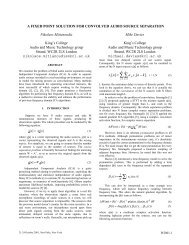
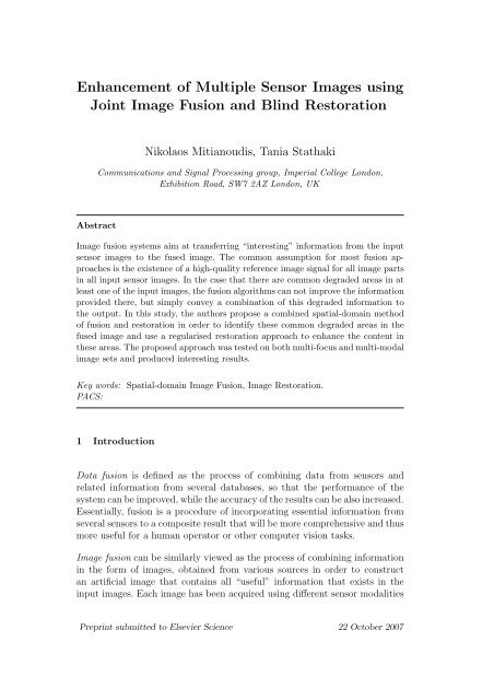
<strong>Enhancement</strong> <strong>of</strong> <strong>Multiple</strong> <strong>Sensor</strong> <strong><strong>Image</strong>s</strong> <strong>using</strong><br />
<strong>Joint</strong> <strong>Image</strong> Fusion and Blind Restoration<br />
Abstract<br />
Nikolaos Mitianoudis, Tania Stathaki<br />
Communications and Signal Processing group, Imperial College London,<br />
Exhibition Road, SW7 2AZ London, UK<br />
<strong>Image</strong> fusion systems aim at transferring “interesting” information from the input<br />
sensor images to the fused image. The common assumption for most fusion approaches<br />
is the existence <strong>of</strong> a high-quality reference image signal for all image parts<br />
in all input sensor images. In the case that there are common degraded areas in at<br />
least one <strong>of</strong> the input images, the fusion algorithms can not improve the information<br />
provided there, but simply convey a combination <strong>of</strong> this degraded information to<br />
the output. In this study, the authors propose a combined spatial-domain method<br />
<strong>of</strong> fusion and restoration in order to identify these common degraded areas in the<br />
fused image and use a regularised restoration approach to enhance the content in<br />
these areas. The proposed approach was tested on both multi-focus and multi-modal<br />
image sets and produced interesting results.<br />
Key words: Spatial-domain <strong>Image</strong> Fusion, <strong>Image</strong> Restoration.<br />
PACS:<br />
1 Introduction<br />
Data fusion is defined as the process <strong>of</strong> combining data from sensors and<br />
related information from several databases, so that the performance <strong>of</strong> the<br />
system can be improved, while the accuracy <strong>of</strong> the results can be also increased.<br />
Essentially, fusion is a procedure <strong>of</strong> incorporating essential information from<br />
several sensors to a composite result that will be more comprehensive and thus<br />
more useful for a human operator or other computer vision tasks.<br />
<strong>Image</strong> fusion can be similarly viewed as the process <strong>of</strong> combining information<br />
in the form <strong>of</strong> images, obtained from various sources in order to construct<br />
an artificial image that contains all “useful” information that exists in the<br />
input images. Each image has been acquired <strong>using</strong> different sensor modalities<br />
Preprint submitted to Elsevier Science 22 October 2007
or capture techniques, and therefore, it has different features, such as type <strong>of</strong><br />
degradation, thermal and visual characteristics. The main concept behind all<br />
image fusion algorithms is to detect strong salient features in the input sensor<br />
images and fuse these details to the synthetic image. The resulting synthetic<br />
image is usually referred to as the fused image.<br />
Let x1(r), . . . , xT (r) represent T images <strong>of</strong> size M1 × M2 capturing the same<br />
scene, where r = (i, j) refers to pixel coordinates (i, j) in the image. Each image<br />
has been acquired <strong>using</strong> different sensors that are placed relatively close<br />
and are observing the same scene. Ideally, the images acquired by these sensors<br />
should be similar. However, there might exist some miscorrespondence<br />
between several points <strong>of</strong> the observed scene, due to the different sensor viewpoints.<br />
<strong>Image</strong> registration is the process <strong>of</strong> establishing point-by-point correspondence<br />
between a number <strong>of</strong> images, describing the same scene. In this<br />
study, the input images are assumed to have negligible registration problems<br />
or the transformation matrix between the sensors’ viewpoints is known. Thus,<br />
the objects in all images can be considered geometrically aligned.<br />
As already mentioned, the process <strong>of</strong> combining the important features from<br />
the original T images to form a single enhanced image y(r) is usually referred<br />
to as image fusion. Fusion techniques can be divided into spatial domain and<br />
transform domain techniques [5]. In spatial domain techniques, the input images<br />
are fused in the spatial domain, i.e. <strong>using</strong> localised spatial features. Assuming<br />
that g(·) represents the “fusion rule”, i.e. the method that combines<br />
features from the input images, the spatial domain techniques can be summarised,<br />
as follows:<br />
y(r) = g(x1(r), . . . , xT (r)) (1)<br />
Moving to a transform domain enables the use <strong>of</strong> a framework, where the<br />
image’s salient features are more clearly depicted than in the spatial domain.<br />
Let T {·} represent a transform operator and g(·) the applied fusion rule.<br />
Transform-domain fusion techniques can then be outlined, as follows:<br />
y(r) = T −1 {g(T {x1(r)}, . . . , T {xT (r)})} (2)<br />
Several transformations were proposed to be used for image fusion, including<br />
the Dual-Tree Wavelet Transform [5,7,12], Pyramid Decomposition [14] and<br />
image-trained Independent Component Analysis bases [10,9]. All these transformations<br />
project the input images onto localised bases, modelling sharp and<br />
abrupt transitions (edges) and therefore, describe the image <strong>using</strong> a more<br />
meaningful representation that can be used to detect and emphasize salient<br />
features, important for performing the task <strong>of</strong> image fusion. In essence, these<br />
transformations can discriminate between salient information (strong edges<br />
2
and texture) and constant or non-textured background and can also evaluate<br />
the quality <strong>of</strong> the provided salient information. Consequently, one can select<br />
the required information from the input images in the transform domain to<br />
construct the “fused” image, following the criteria presented earlier on.<br />
In the case <strong>of</strong> multi-focus image fusion scenarios, an alternative approach<br />
has been proposed in the spatial domain, exploiting current error estimation<br />
methods to identify high-quality edge information [6]. One can perform error<br />
minimization between the fused and input images, <strong>using</strong> various proposed error<br />
norms in the spatial domain in order to perform fusion. The possible benefit<br />
<strong>of</strong> a spatial-domain approach is the reduction in computational complexity,<br />
which is present in a transform-domain method due to the forward and inverse<br />
transformation step.<br />
In addition, following a spatial-domain fusion framework, one can also benefit<br />
from current available spatial-domain image enhancement techniques to<br />
incorporate a possible restoration step to enhance areas that exhibit distorted<br />
information in all input images. Current fusion approaches can not enhance<br />
areas that appear degraded in any sense in all input images. There is a necessity<br />
for some pure information to exist for all parts <strong>of</strong> the image in the various<br />
input images, so that the fusion algorithm can produce a high quality output.<br />
In this work, we propose to reformulate and extend Jones and Vorontsov’s [6]<br />
spatial-domain approach to fuse the non-degraded common parts <strong>of</strong> the sensor<br />
images. A novel approach is used to identify the areas <strong>of</strong> common degradation<br />
in all input sensor images. A double-regularised image restoration approach<br />
<strong>using</strong> robust functionals is applied on the estimated common degraded area<br />
to enhance the common degraded area in the “fused” image. The overall fusion<br />
result is superior to any traditional fusion approach since the proposed<br />
approach goes beyond the concept <strong>of</strong> transferring useful information to a thorough<br />
fusion-enhancement approach.<br />
2 Robust Error Estimation Theory<br />
Let the image y(r) be a recovered version from a degraded observed image<br />
x(r), where r = (i, j) are pixel coordinates (i, j). To estimate the recovered<br />
image y(r), one can minimise an error functional E(y) that expresses the<br />
difference between the original image and the estimated one, in terms <strong>of</strong> y.<br />
The error functional can be defined by:<br />
<br />
E(y) = ρ (r, y(r), |∇y(r)|) dr (3)<br />
Ω<br />
3
where Ω is the image support, ∇y(r) is the image gradient. The function ρ(·)<br />
is termed the error norm and is defined according to the application, i.e. the<br />
type <strong>of</strong> degradation or the desired task. For example, a least square error norm<br />
can be appropriate to remove additive Gaussian noise from a degraded image.<br />
The extremum <strong>of</strong> the previous equation can be estimated, <strong>using</strong> the Euler -<br />
Lagrange equation. The Euler-Lagrange equation is an equation satisfied by a<br />
function f <strong>of</strong> a parameter t which extremises the functional:<br />
<br />
E(f) = F (t, f(t), f ′ (t)) dt (4)<br />
where F is a given function with continuous first partial derivatives. The Euler-<br />
Lagrange equation is described by the following ordinary differential equation,<br />
i.e. a relation that contains functions <strong>of</strong> only one independent variable, and<br />
one or more <strong>of</strong> its derivatives with respect to that variable, the solution t <strong>of</strong><br />
which extremises the above functional [21].<br />
∂<br />
∂f(t) F (t, f(t), f ′ (t)) − d<br />
dt<br />
∂<br />
∂f ′ (t) F (t, f(t), f ′ (t)) = 0 (5)<br />
Applying the above rule to derive the extremum <strong>of</strong> (3), the following Euler-<br />
Lagrange equation is derived:<br />
∂ρ<br />
∂y − ∇ ∂ρ <br />
= 0 (6)<br />
∂∇y<br />
Since ρ(·) is a function <strong>of</strong> |∇y| and not ∇y, we perform the substitution<br />
∂∇y = ∂|∇y|/sgn(∇y) = |∇y|∂|∇y|/∇y (7)<br />
where sgn(y) = y/|y|. Consequently, the Euler-Lagrange equation is given by:<br />
∂ρ<br />
∂y − ∇ 1<br />
|∇y|<br />
∂ρ<br />
∂|∇y| ∇y(r) = 0 (8)<br />
To obtain a closed-form solution y(r) from (8) is not straightforward. Hence,<br />
one can use numerical optimisation methods to estimate y. Gradient-descent<br />
optimisation can be applied to estimate y(r) iteratively <strong>using</strong> the following<br />
update rule:<br />
∂y(r, t)<br />
y(r, t) ← y(r, t − 1) − η<br />
∂t<br />
4<br />
(9)
where t is the time evolution parameter, η is the optimisation step size and<br />
∂y(r, t)<br />
∂t<br />
= −∂ρ<br />
∂y + ∇ 1<br />
|∇y|<br />
∂ρ<br />
∇y(r, t)<br />
∂|∇y|<br />
(10)<br />
Starting with the initial condition y(r, 0) = x(r), the iteration <strong>of</strong> (10) continues<br />
until the minimisation criterion is satisfied, i.e. |∂y(r, t)/∂t| < ɛ, where ɛ is a<br />
small constant (ɛ ∼ 0.0001). In practice, only a finite number <strong>of</strong> iterations are<br />
performed to achieve visually satisfactory results [6]. The choice <strong>of</strong> the error<br />
norm ρ(·) in the Lagrange-Euler equation is the next topic <strong>of</strong> discussion.<br />
2.1 Isotropic diffusion<br />
As mentioned previously, one candidate error norm ρ(·) is the least-squares<br />
error norm. This norm is given by:<br />
ρ(r, |∇y(r)|) = 1<br />
2 |∇y(r)|2<br />
(11)<br />
The above error norm smooths Gaussian noise and depends only on the image<br />
gradient ∇y(r), but not explicitly on the image y(r) itself. If the least-squares<br />
error norm is substituted in the time evolution equation (10), we get the<br />
following update:<br />
∂y(r, t)<br />
∂t = ∇2 y(r, t) (12)<br />
which is the isotropic diffusion equation having the following analytic solution<br />
[2]:<br />
y(r, t) = G(r, t) ∗ x(r) (13)<br />
where ∗ denotes the convolution <strong>of</strong> a Gaussian function G(r, t) <strong>of</strong> standard<br />
deviation t with x(r), the initial data. The solution specifies that the time<br />
evolution in (12) is a convolution process performing Gaussian smoothing.<br />
However, as the time evolution iteration progresses, the function y(r, t) becomes<br />
the product <strong>of</strong> the convolution <strong>of</strong> the input image with a Gaussian <strong>of</strong><br />
constantly increasing variance, which will finally produce a constant value.<br />
In addition, it has been shown that isotropic diffusion may not only smooth<br />
edges, but also causes drifts <strong>of</strong> the actual edges in the image edge, because<br />
<strong>of</strong> the Gaussian filtering (smoothing) [2,13]. These are two disadvantages that<br />
need to be seriously considered when <strong>using</strong> isotropic diffusion.<br />
5
2.2 Isotropic diffusion with edge enhancement<br />
<strong>Image</strong> fusion aims at transferring salient features to the fused image. In this<br />
work and in most fusion systems, saliency is interpreted as edge information<br />
and therefore, image fusion aims at highlighting edges in the fused image. An<br />
additional desired property can be to smooth out any possible Gaussian noise.<br />
In order to achieve the above tasks <strong>using</strong> an error estimation framework, the<br />
objective is to create an error norm that will enhance edges in an image and<br />
simultaneously smooth possible noise. The following error norm, combining<br />
isotropic smoothing with edge enhancement, was proposed in [6]:<br />
ρ(r, y(r, t), |∇y(r, t)|) = α<br />
2 |∇y(r, t)|2 + β<br />
2 Jx(r)(y(r, t) − x(r)) 2<br />
(14)<br />
where α, β are constants that define the level <strong>of</strong> smoothing and edge enhancement<br />
respectively that is performed by the cost function, t is the time<br />
evolution and Jx is commonly termed the anisotropic gain function, which<br />
is a Gaussian smoothed edge map. One possible choice for implementing a<br />
Gaussian smoothed edge map is the following :<br />
<br />
Jx(r) = κ<br />
|∇x(q)| 2 G(r − q, σ)d 2 q (15)<br />
where G(·) is a Gaussian function <strong>of</strong> zero-mean and standard deviation σ and<br />
κ is a constant. Another choice can be a smoothed Laplacian edge map. The<br />
anisotropic gain function has significantly higher values around edges or where<br />
sharp features are dominant compared to blurred or smooth regions.<br />
Substituting the above error norm into the gradient descent update <strong>of</strong> (10)<br />
yields the following time evolution equation with anisotropic gain:<br />
∂y(r, t)<br />
∂t = α∇2 y(r, t) − βJx(r)(y(r, t) − x(r)) (16)<br />
The above equation essentially smoothes noise while enhancing edges. The<br />
parameters α and β control the effects <strong>of</strong> each term. The parameter α controls<br />
the amount <strong>of</strong> noise smoothing in the image and β controls the anisotropic<br />
gain, i.e. the preservation and enhancement <strong>of</strong> the edges. For noiseless images,<br />
an evident choice is α = 0 and β = 1. In this case, for short time intervals, the<br />
anisotropic gain function Jx induces significant changes dominantly around<br />
regions <strong>of</strong> sharp contrast, resulting in edge enhancement.<br />
There is always a possibility that in some regions <strong>of</strong> interest, the anisotropic<br />
gain function is not high enough and therefore the above update rule can<br />
6
potentially degrade the quality <strong>of</strong> information that is already integrated into<br />
the input image and consequently in the enhanced image. To prevent such<br />
erasing effects, however small might be, John and Vorontsov [6] introduced<br />
the following modified anisotropic gain function:<br />
J(r, t) = Jx(r) − Jy(r, t) (17)<br />
The general update formula to estimate f(r) becomes then:<br />
∂y(r, t)<br />
∂t = α∇2 y(r, t) − Θ(J(r, t))J(r, t)(y(r, t) − x(r)) (18)<br />
where<br />
⎧<br />
⎪⎨ 1 , J ≥ 0<br />
Θ(J) =<br />
⎪⎩ 0 , J < 0<br />
(19)<br />
The new term Θ(J)J allows only high quality information, interpreted in<br />
terms <strong>of</strong> edge presence, to transfer to the enhanced image. In the opposite case<br />
that Jx(r) < Jy(r), the information in the enhanced image has better edge<br />
representation than the original degraded image for several r and therefore, no<br />
processing is necessary. In the case <strong>of</strong> a single input image, the above concept<br />
might not seem practical. In the following section, the proposed concept is<br />
employed in a multiframe input scenario, where the aim is to transfer only high<br />
quality information to the enhanced image y(r). In this case, this positive edge<br />
injection mechanism is absolutely vital to ensure information enhancement.<br />
3 Fusion with Error Estimation theory<br />
In this section, the authors propose a novel spatial-domain fusion algorithm,<br />
based on the basic formulation <strong>of</strong> John and Vorontsov. In [6], a sequential<br />
approach to image fusion based on Error Estimation theory was proposed.<br />
Assuming that we have a number <strong>of</strong> T input frames xn(r) to be fused, one can<br />
easily perform selective image fusion, by iterating the update rule (18) for the<br />
estimation <strong>of</strong> y(r) <strong>using</strong> each <strong>of</strong> input images xn consecutively for a number <strong>of</strong><br />
K iterations. In a succession <strong>of</strong> intervals <strong>of</strong> K iterations, the synthetic frame<br />
finally integrates high-quality edge areas from the entire set <strong>of</strong> input frames.<br />
The possibility <strong>of</strong> data fusion occurring in regions where the anisotropic gain<br />
function is not high enough, can potentially degrade quality information already<br />
integrated into the synthetic frame. To prevent such erasing effects, as<br />
7
mentioned in the previous section, a differential anisotropic gain function can<br />
be introduced to transfer only high quality information to the fused image<br />
y(r). The proposed approach by John and Vorontsov can be applied mainly<br />
in the case <strong>of</strong> a video stream, where the quality <strong>of</strong> the observed image is enhanced,<br />
based on previous and forthcoming frames. However, this framework<br />
is not efficient in the case <strong>of</strong> fusion applications, where the input frames are<br />
simultaneously available for processing and fusion. In this case, a reformulation<br />
<strong>of</strong> the above procedure is needed and is described in full in the following<br />
section.<br />
3.1 A novel fusion formulation based on error estimation theory<br />
Assume there are T images xn(r) that capture the same observed scene. The<br />
input images are assumed to be registered and each image contains exactly<br />
the same scene. This assumption is valid, since in most real-life applications,<br />
the input sensors are arranged in a close-distance array and similar zoom level<br />
in order to minimise the need for registration or the viewpoint transformation<br />
matrix is known. Different parts <strong>of</strong> the images are blurred <strong>using</strong> different<br />
amounts and types <strong>of</strong> blur. The objective is to combine the useful parts <strong>of</strong><br />
input information to form a composite (“fused”) image.<br />
The described setup can model a possible out-<strong>of</strong>-focus scenario <strong>of</strong> image capture.<br />
We have all witnessed the case, where we want to take a photograph <strong>of</strong><br />
an object in a scene and the camera focuses on a background point/object by<br />
mistake. As a result, the foreground object appears blurred in the final image,<br />
whereas the background texture is properly captured. In a second attempt to<br />
photograph the object correctly, the foreground object appears properly and<br />
the background appears blurred. Ideally, we would like to combine the two<br />
images into a new one, where everything would appear in full detail. This is<br />
an example <strong>of</strong> a real-life application for the fusion <strong>of</strong> out-<strong>of</strong>-focus images. The<br />
same scenario can also appear in military surveillance and general surveillance<br />
applications, where one would like to enhance the surveillance output,<br />
by combining multiple camera inputs at different focal length.<br />
The fused image y(r, t) can be constructed as a linear combination <strong>of</strong> the T<br />
input registered images xn(r). The fusion problem is usually solved by finding<br />
the weights wn(r, t) that transfer all the useful information from the input<br />
images xn to the fused image y [10,9].<br />
y(r, t) = w1(r, t)x1(r) + . . . + wT (r, t)xT (r) (20)<br />
where wn(r, t) denotes the n th weight <strong>of</strong> the image xn at position r. To estimate<br />
these weights, we can perform error minimisation <strong>using</strong> the previously<br />
8
mentioned approach <strong>of</strong> Isotropic Diffusion with edge enhancement. The problem<br />
is now to estimate the weights wn simultaneously, so as to achieve edge<br />
preservation. This cannot be accomplished directly by the scheme proposed<br />
by Jones and Vorontsov.<br />
In other words, we need to estimate the derivative ∂wn/∂t simultaneously, for<br />
all n = 1, . . . , T . We can associate ∂wn/∂t with ∂y/∂t that has already been<br />
derived before.<br />
∂y<br />
∂t<br />
∂y ∂wn<br />
=<br />
∂wn ∂t<br />
∂wn<br />
= xn<br />
∂t<br />
(21)<br />
Therefore, we can use the previous update rule to estimate the contribution<br />
<strong>of</strong> each image to the fused one:<br />
∂wn(r, t)<br />
∂t<br />
= 1 ∂y(r, t)<br />
xn(r) ∂t<br />
(22)<br />
The fusion weight wn(r, t) <strong>of</strong> each input image can then be estimated <strong>using</strong><br />
sequential minimisation with the following update rule ∀n = 1, . . . , T :<br />
where<br />
wn(r, t + 1) ← wn(r, t) − η ∂wn(r, t)<br />
∂t<br />
∂wn(r, t)<br />
∂t<br />
(23)<br />
= − 1<br />
xn(r) Θ(Jn(r, t))Jn(r, t)(y(r, t) − xn(r)) (24)<br />
and Jn(r, t) = Jxn(r) − Jy(r, t). To avoid possible numerical instabilities, for<br />
those r that xn(r) = 0, a small constant is added to these elements so as to<br />
become nonzero. All weights are initialised to wn(r, t) = 1/T , which represents<br />
the “mean” fusion rule. As this scheme progresses over time, the weights are<br />
adapting and tend to emphasise more the useful details that exist in each<br />
image and suppress the information that is not very accurate. In addition, all<br />
the fusion weights are estimated simultaneously <strong>using</strong> this scheme. Therefore,<br />
after a couple <strong>of</strong> iterations the majority <strong>of</strong> the useful information is extracted<br />
from the input images and transferred to the composite image.<br />
3.2 Fusion experiments <strong>of</strong> out-<strong>of</strong>-focus and multimodal image sets <strong>using</strong> error<br />
estimation theory<br />
In this section, we perform several fusion experiments <strong>of</strong> both out-<strong>of</strong>-focus and<br />
multimodal images to evaluate the performance <strong>of</strong> the proposed approach.<br />
9
Petrovic Piella<br />
TopoICA 0.6151 0.9130<br />
Fusion with EE 0.6469 0.9167<br />
Table 1<br />
Performance evaluation <strong>of</strong> the Diffusion approach and the TopoICA-based fusion<br />
approach <strong>using</strong> Petrovic [18] and Piella’s [15] metrics.<br />
Most test images were taken from the <strong>Image</strong> Fusion server [3]. The numerical<br />
evaluation in most experiments was performed <strong>using</strong> the indexes proposed by<br />
Piella [15] and Petrovic [18].<br />
In the first experiment, the system is tested with an out-<strong>of</strong>-focus example, the<br />
“Disk” dataset. The ICA-based fusion algorithm, proposed in [10], was employed<br />
as a benchmark to the new proposed algorithm. We used 40 TopoICA<br />
8×8 bases, trained from 10000 patches that were randomly selected from natural<br />
images. Then, the “Weighted Combination” rule was selected to perform<br />
fusion <strong>of</strong> the input images. On the other hand, for the spatial-domain fusion<br />
scheme, the parameters were set to α = 0 (no visible noise), β = 0.8 and the<br />
learning parameter was set to η = 0.08. The Gaussian smoothed edge map <strong>of</strong><br />
(15) was calculated by extracting an edge map <strong>using</strong> the Sobel mask, which<br />
was subsequently smoothed by a Gaussian 5 × 5 kernel <strong>of</strong> standard deviation<br />
σ = 1. The fusion results <strong>of</strong> the two methods are depicted in Figure 1. We<br />
notice that the proposed approach produces sharper edges compared to the<br />
ICA-Based method. The difference is more visible around the edges <strong>of</strong> the<br />
tilted books in the bookcase and the eye on the cover <strong>of</strong> the book that is<br />
in front <strong>of</strong> the bookcase. In Figure 2, the convergence rate <strong>of</strong> the estimation<br />
<strong>of</strong> one <strong>of</strong> the fusion weights is shown. The proposed algorithm demonstrates<br />
almost linear convergence, which is expected for a gradient algorithm.<br />
In Table 1, the performance <strong>of</strong> the proposed method is compared with the<br />
ICA-based method, in terms <strong>of</strong> the Petrovic and Piella method. The metrics<br />
give slightly higher performance to the proposed methodology. However, we<br />
can observe an improvement in the visual representation <strong>of</strong> edges <strong>using</strong> the<br />
proposed method in the particular application <strong>of</strong> fusion <strong>of</strong> out-<strong>of</strong>-focus images.<br />
The estimated fusion weights w1(r), w2(r) are depicted in Figure 3. It is clear<br />
that the weights w1, w2 highlight the position <strong>of</strong> high-quality information in<br />
the input images. The cost function that is optimised in this case aims at<br />
highlighting edges in the “fused” image. This is essentially what is estimated<br />
by the weight maps w1(r), w2(r). This information can be used to identify<br />
common areas <strong>of</strong> inaccurate information in the input images. A restoration<br />
algorithm could be applied to these areas and enhance the final information<br />
that is conveyed to the “fused” image.<br />
The next step is to apply the proposed algorithm to a multimodal scenario.<br />
10
(a) Input <strong>Image</strong> 1 (b) Input <strong>Image</strong> 2<br />
(c) TopoICA Fusion (d) Proposed Scheme<br />
(e) TopoICA Fusion (f) Proposed Scheme<br />
Fig. 1. An out-<strong>of</strong>-focus fusion example <strong>using</strong> the “Disk” dataset available by the<br />
<strong>Image</strong> Fusion server [3]. We compare the TopoICA-based fusion approach and the<br />
proposed Diffusion scheme.<br />
We will use an image pair from the “Dune” dataset <strong>of</strong> surveillance images from<br />
TNO Human Factors, provided by L. Toet [16] in the <strong>Image</strong>Fusion Server [3].<br />
We applied the TopoICA-based approach [10] <strong>using</strong> the “maxabs” fusion rule<br />
and the proposed algorithm on the dataset, <strong>using</strong> the same settings as in the<br />
previous example. In Figure 4, we plot the fused results <strong>of</strong> the two methods<br />
and in Table 2, we plot their numerical evaluation <strong>using</strong> Petrovic and Piella’s<br />
indexes.<br />
According to the performance evaluation indexes, the ICA-based approach<br />
performs considerably better than the proposed approach. The same trend<br />
is also observed in the metrics. However, the proposed approach performs<br />
11
||∂ w 1 /∂ t|| 2<br />
x 104<br />
9<br />
8<br />
7<br />
6<br />
5<br />
4<br />
3<br />
2<br />
1<br />
0<br />
0 50 100<br />
Iterations<br />
150 200<br />
Fig. 2. Convergence <strong>of</strong> the estimated fusion weight w1 <strong>using</strong> the proposed fusion<br />
algorithm in terms <strong>of</strong> ||∂w1/∂t|| 2 .<br />
(a) Estimated w1(r) (b) Estimated w2(r)<br />
Fig. 3. The weights w1, w2 highlight the position <strong>of</strong> high quality information in the<br />
input images.<br />
Petrovic Piella<br />
TopoICA 0.4921 0.7540<br />
Fusion with EE 0.4842 0.6764<br />
Table 2<br />
Performance evaluation in the case <strong>of</strong> a multimodal example from the Toet database.<br />
The TopoICA-based approach is compared with the proposed fusion approach.<br />
differently to a common fusion approach. It aims at highlighting the edges <strong>of</strong><br />
the input images to the fused image, due to the edge enhancement term in<br />
the cost function. This is can be observed directly in Figure 4(d). All edges<br />
and texture areas are highly enhanced in the fused image together with the<br />
outline <strong>of</strong> the important target, i.e. the hidden man in the middle <strong>of</strong> the<br />
picture. Consequently, one should also consult the human operators <strong>of</strong> modern<br />
fusion systems, apart from proposed fusion metrics [15,18], in order to evaluate<br />
efficiently the performance <strong>of</strong> these algorithms. Perhaps the outlined fusion<br />
result is more appealing to human operators and the human vision system in<br />
general and therefore may be also be examined as a preferred solution.<br />
12
(a) Input <strong>Image</strong> 1 (b) Input <strong>Image</strong> 2<br />
(c) TopoICA Fusion (d) Proposed Scheme<br />
Fig. 4. Comparison <strong>of</strong> a multimodal fusion example <strong>using</strong> the TopoICA method and<br />
the Diffusion approach. Even though the metrics demonstrate worse performance,<br />
the diffusion approach highlights edges giving a sharper fused image.<br />
4 <strong>Joint</strong> <strong>Image</strong> Fusion and Restoration<br />
The basic <strong>Image</strong> Fusion concept assumes that there is some useful information<br />
for all parts <strong>of</strong> the observed scene at least in one <strong>of</strong> the input sensors. However,<br />
this assumption might not always be true. This means that there might be<br />
parts <strong>of</strong> the observed scene where there is only degraded information available.<br />
The current fusion algorithms will fuse all high quality information from the<br />
input sensors and for the common degraded areas will form a blurry mixture<br />
<strong>of</strong> the input images, as there is no high quality information available.<br />
In the following section, the problem <strong>of</strong> identifying the areas <strong>of</strong> common degraded<br />
information in all input images is addressed. A mechanism is established<br />
for identifying common degraded areas in an image. Once this part is<br />
identified, an image restoration approach can be applied as a second step in<br />
order to enhance these parts for the final composite “fused” image.<br />
4.1 Identifying common degraded areas in the sensor images<br />
The first task will be to identify the areas <strong>of</strong> degraded information in the input<br />
sensor images. An identification approach, based on local image statistics, will<br />
13
e pursued to trace the degraded areas.<br />
The “fused” image will be employed, as it emerges from the fusion algorithm.<br />
As mentioned earlier, the fusion algorithm will attempt to merge the areas<br />
<strong>of</strong> high detail to the fused image, whereas for the areas <strong>of</strong> degraded information,<br />
i.e. areas <strong>of</strong> weak edges or texture in all input images, will not impose<br />
any preference to any <strong>of</strong> the input images and therefore the estimated fusion<br />
weights will remain approximately equal to the initial weights wi = 1/T . Consequently,<br />
the areas <strong>of</strong> out-<strong>of</strong>-focus distortion will be described by areas <strong>of</strong> low<br />
edge information in the fused image. Equivalently, some areas <strong>of</strong> very low texture<br />
or constant background also need to be excluded, since there is no benefit<br />
in restoring them. These areas can be traced, by evaluating the local standard<br />
deviation <strong>of</strong> an edge information metric in small local neighbourhoods around<br />
each pixel. The following algorithm for extracting common degraded areas is<br />
described in the following steps:<br />
(1) Extract an edge map <strong>of</strong> the fused image f, <strong>using</strong> the Laplacian kernel,<br />
i.e. ∇ 2 f(r, t).<br />
(2) Find the local standard deviations VL(r, t) for each pixel <strong>of</strong> the Laplacian<br />
edge map ∇ 2 f(r, t), <strong>using</strong> 5 × 5 local neighbourhoods.<br />
(3) Reduce the dynamic range by calculating ln(VL(r, t)).<br />
(4) Estimate VsL(r, t), by smoothing ln(VL(r, t)) <strong>using</strong> a 15×15 median filter.<br />
(5) Create the common degraded area map A(r) by thresholding VsL(r, t).<br />
The mask A(r) is set to 1, for those r that q minr(VsL(r, t)) < VsL(r, t) <<br />
pmeanr(VsL(r, t)), otherwise is set to zero.<br />
Essentially, we create an edge map, as described by the Laplacian kernel. The<br />
Laplacian kernel was chosen because it was already estimated during the fusion<br />
stage <strong>of</strong> the framework. The next step is to find the local activity in<br />
5 × 5 neighbourhoods around each pixel in the edge map. A metric <strong>of</strong> local<br />
activity is given by the local standard deviation. A pixel <strong>of</strong> high local activity<br />
should be part <strong>of</strong> an “interesting” detail in the image (edge, strong texture<br />
etc), whereas a point <strong>of</strong> low local activity might be a constant background<br />
or weak texture pixel. We can devise a heuristic thresholding scheme in order<br />
to identify these areas <strong>of</strong> weak local activity, i.e. possible degraded areas in<br />
all input images for fusion. The next step is to reduce the dynamic range <strong>of</strong><br />
these measurements, <strong>using</strong> a logarithmic nonlinear mapping, such as ln(·). To<br />
smooth out isolated pixels and connect similar areas, we perform median filtering<br />
<strong>of</strong> the log-variance map. Consequently, the common degraded area map<br />
is created by thresholding the values <strong>of</strong> the log-variance map with a heuristic<br />
threshold set to q minr(VsL(r, t)) < VsL(r, t) < pmeanr(VsL(r, t)), where p, q<br />
are constants. The aim is to avoid high quality edge/texture and constant<br />
background information. The level <strong>of</strong> detail along with the level <strong>of</strong> constant<br />
background differ for different images. In order to identify the common degraded<br />
area with accuracy, the parameters p, q need to be defined manually for<br />
14
(a) Input <strong>Image</strong> 1 (b) Input <strong>Image</strong> 2<br />
(c) Fusion Scheme (d) VsL(r) (e) Degraded area map<br />
Fig. 5. If there exist blurry parts in all input images, common <strong>Image</strong> Fusion algorithms<br />
cannot enhance these parts, but will simply transfer the degraded information<br />
to the fused image. However, this area <strong>of</strong> degraded information is still<br />
identifiable<br />
each image. The parameter q defines the level <strong>of</strong> background information that<br />
needs to be removed. In a highly active image, q is usually set to 1, however,<br />
other values have to be considered for images with large constant background<br />
areas. The parameter p is the upper bound threshold to discriminate between<br />
strong edges and weak edges, possibly belonging to a common degraded area.<br />
Setting p around the mean edge activity, we can find a proper threshold for<br />
the proposed system. Values that were found to work well in experiments<br />
were q ∈ [0.98, 1] and p ∈ [1, 1.1]. Some examples <strong>of</strong> common degraded area<br />
identification <strong>using</strong> the above technique are shown in Figures 5, 6.<br />
4.2 <strong>Image</strong> restoration<br />
A number <strong>of</strong> different approaches for tackling the image restoration problem<br />
have been proposed in the literature, based on various principles. For<br />
an overview <strong>of</strong> image restoration methods, one can always possibly refer to<br />
Kundur and Hatzinakos [8] and Andrews and Hunt [1]. In this study, the<br />
double-weighted regularised image restoration approach in the spatial domain<br />
is pursued, that was initially proposed by You and Kaveh [19], with additional<br />
robust functionals to improve the performance in the case <strong>of</strong> outliers.<br />
The restoration problem is described by the following model:<br />
y(r) = h(r) ∗ f(r) + d(r) (25)<br />
15
(a) Input <strong>Image</strong> 1 (b) Input <strong>Image</strong> 2<br />
(c) Fusion Scheme (d) VsL(r) (e) Degraded area map<br />
Fig. 6. Another example <strong>of</strong> degraded area identification in “fused” images.<br />
where ∗ denotes 2D convolution, h(r) the degradation kernel, f(r) the estimated<br />
image and d(r) possible additive noise.<br />
4.2.1 Double weighted regularised image restoration<br />
Conventional double weighted regularization for blind image restoration [1]<br />
estimates the original image by minimizing the cost function Q(h(r), f(r)) <strong>of</strong><br />
the following quadratic form:<br />
Q(h(r), f(r)) = 1<br />
2 ||A1(r) (y(r) − h(r) ∗ f(r)) || 2<br />
<br />
residual<br />
+ λ<br />
2 ||A2(r) (Cf ∗ f(r)) || 2<br />
<br />
image regularisation<br />
+ γ<br />
2 ||A3(r) (Ch ∗ h(r)) || 2<br />
<br />
blur regularisation<br />
(26)<br />
where || · || represents the L2-norm. The above cost function has three distinct<br />
terms. The residual term, the first term on the right-hand side <strong>of</strong> (26),<br />
represents the accuracy <strong>of</strong> the restoration process. This term is similar to a<br />
second-order error-norm (least-squares estimation), as described in a previous<br />
paragraph. The second term, called the regularising term, imposes a smoothness<br />
constraint on the recovered image and the third term acts similarly to the<br />
estimated blur. Additional constraints must be imposed, including the non-<br />
16
negativity and finite-support constraint for both the blurring kernel and the<br />
image. Besides, the blurring kernel must always preserve the energy, i.e. all the<br />
coefficients should sum to 1. The regularization operators Cf and Ch are highpass<br />
Laplacian operators applied on the image and the PSF respectively. The<br />
functions A1, A2 and A3 represent spatial weights for each optimisation term.<br />
The parameters λ and γ control the trade-<strong>of</strong>f between the residual term and<br />
the corresponding regularising terms for the image and the blurring kernel.<br />
One can derive the same cost function through a Bayesian framework <strong>of</strong> estimating<br />
f(r) and h(r). To illustrate this connection, we assume that the<br />
blurring kernel h(r) is known and the aim is to recover f(r). A Maximum-A-<br />
Posteriori (MAP) estimate <strong>of</strong> f(r) is given by performing maxf log p(y, f|r) =<br />
maxf log p(y|f, r)p(f|r), where r denotes the observed samples. Assuming Gaussian<br />
noise for d(r), we have that p(y|f, r) ∝ exp (−0.5a||y(r) − h(r) ∗ f(r)|| 2 ).<br />
Assuming smoothness for the image pr<strong>of</strong>ile, one can employ the image prior<br />
p(f|r) ∝ exp (−0.5b||Cf ∗ f(r)|| 2 ), which has been widely used by the engineering<br />
community [11] in setting constraints on first or second differences,<br />
i.e. restricting the rate <strong>of</strong> changes in an image (a, b are constants that can<br />
determine the shape <strong>of</strong> the prior). Using the proposed models, one can derive<br />
a MAP estimate by optimising a function that is the same as the first two<br />
terms <strong>of</strong> (26), illustrating the connection between the two approaches.<br />
To estimate f(r) and h(r), the above cost function needs to be minimised.<br />
Since each term <strong>of</strong> the cost function is quadratic, it can simply be optimized by<br />
applying alternating Gradient Descent optimisation [1]. This implies that the<br />
estimates for the image and the PSF can be estimated alternatively, <strong>using</strong> the<br />
gradients <strong>of</strong> the cost function with respect to f(r) and h(r). More specifically,<br />
the double iterative scheme can be expressed, as follows:<br />
• At each iteration, update:<br />
∂Q(h(t), f(t))<br />
f(t + 1) = f(t) − η1<br />
∂f(t)<br />
∂Q(h(t), f(t + 1))<br />
h(t + 1) = h(t) − η2<br />
∂h(t)<br />
• Stop, if f and h converge.<br />
(27)<br />
(28)<br />
The terms η1 and η2 are the step size parameters that control the convergence<br />
rates for the image and Point Spread Function (PSF) (blurring kernel)<br />
respectively. After setting the initial estimate <strong>of</strong> the image as the degraded<br />
image, and the PSF as a random mask, the cost function is differentiated with<br />
respect to the image first, while the PSF is kept constant, and vice versa. The<br />
required derivatives <strong>of</strong> the cost function are presented below:<br />
17
∂Q(h, f)<br />
= −A1(r)h(−r) ∗ (y(r) − h(r) ∗ f(r))<br />
∂f<br />
+ λ <br />
A2(r)C T f ∗ (Cf ∗ f(r)) <br />
∂Q(h, f)<br />
∂h<br />
= −A1(r)f(−r) ∗ (y(r) − h(r) ∗ f(r))<br />
+ γ <br />
A3(r)C T h ∗ (Ch ∗ h(r)) <br />
(29)<br />
(30)<br />
where the superscript T denotes the transpose operation. Substituting (29)<br />
and (30) into (27) and (28) yields the final form <strong>of</strong> the algorithm (27) and<br />
(28), where the corresponding functions are iterated until convergence.<br />
4.2.2 Robust functionals to the restoration cost function<br />
There exist several criticisms regarding the conventional double regularisation<br />
restoration approach. One is the non-robustness <strong>of</strong> the least squares estimators<br />
employed in the traditional residual term, once the assumption <strong>of</strong><br />
Gaussian noise does not hold [20]. Moreover, the quadratic regularising term<br />
penalises sharp gray-level transitions, due to the linearity <strong>of</strong> the derivative <strong>of</strong><br />
the quadratic function. This implies that sudden changes in the image are filtered,<br />
and thus, the image edges are blurred. To alleviate this problem, we can<br />
introduce robust functionals in the cost function, in order to rectify some <strong>of</strong><br />
the problems <strong>of</strong> this estimator. Therefore, the original cost function becomes:<br />
Q(h(r), f(r)) = 1<br />
2 ||A1(r)ρn (y(r) − h(r) ∗ f(r)) || 2<br />
+ λ<br />
2 ||A2(r)ρf (Cf ∗ f(r)) || 2<br />
+ γ<br />
2 ||A3(r)ρd (Ch ∗ h(r)) || 2<br />
(31)<br />
Three distinct robust kernels ρn(·), ρf(·) and ρd(·) are introduced in the new<br />
cost function and are referred to as the robust residual and regularizing terms<br />
respectively. The partial derivatives <strong>of</strong> the cost function take the following<br />
form:<br />
∂Q(h, f)<br />
∂f<br />
= −A1(r)h(−r) ∗ ρ ′ n (y(r) − h(r) ∗ f(r))<br />
+ λ <br />
A2(r)C T f ∗ ρ ′ f (Cf ∗ f(r)) <br />
18<br />
(32)
∂Q(h, f)<br />
= −A1(r)f(−r) ∗ ρ<br />
∂h<br />
′ n (y(r) − h(r) ∗ f(r))<br />
+ γ <br />
A3(r)C T h ∗ ρ ′ d (Ch ∗ h(r)) <br />
(33)<br />
Robust estimation is usually presented in terms <strong>of</strong> the influence function<br />
l(r) = ∂ρ/∂r. The influence function characterises the bias <strong>of</strong> a particular<br />
measurement on the solution. Traditional least squares kernels fail to eliminate<br />
the effect <strong>of</strong> outliers, with linearly increasing and non-bounded influence<br />
functions. On the other hand, they also tend to over-smooth the image’s details,<br />
since such edge discontinuities lead to large values <strong>of</strong> smoothness error.<br />
Thus, two different kernel types are investigated, in order to increase the robustness<br />
and reject outliers in the context <strong>of</strong> the blind estimation.<br />
To suppress the effect <strong>of</strong> extreme noisy samples (“outliers”) that might be<br />
present in the observations, the derivative <strong>of</strong> an ideal robust residual term<br />
should increase less rapidly than a quadratic term in the case <strong>of</strong> outliers. One<br />
candidate function can be the following:<br />
ρ ′ n(x) =<br />
1<br />
1 + ( x<br />
θ )2υ<br />
(34)<br />
Obviously, the specific function associated with the residual term assists in<br />
suppressing the effect <strong>of</strong> large noise values in the estimation process, by setting<br />
the corresponding influence function to small values. Optimal values for the θ<br />
and υ parameters have been investigated in [4]. These parameters determine<br />
the “shape” <strong>of</strong> the influence function and as a consequence the filtering <strong>of</strong><br />
outliers.<br />
In order to find a trade-<strong>of</strong>f between noise elimination and preservation <strong>of</strong><br />
high-frequency details, the influence functional for the image regularising term<br />
must approximate the quadratic structure at small to moderate values and<br />
alternatively deviate from the quadratic structure at high values, so that the<br />
sharp changes will not be greatly penalised. One possible formulation <strong>of</strong> the<br />
image regularising term is expressed by the absolute entropy function shown<br />
below, which reduces the relative penalty ratio between large and small signal<br />
deviations, compared with the quadratic function [20]. Hence, the absolute<br />
entropy function produces sharper boundaries than the quadratic one, and<br />
therefore can be employed for blind restoration.<br />
ρf(x) = (|x| + e −1 )ln(|x| + e −1 ) (35)<br />
ρ ′ f(x) = 1 <br />
sgn(x) ln(|x| + e<br />
2 −1 ) + 1 <br />
(36)<br />
For simplicity, the robust functional for the stabilising term <strong>of</strong> the Point Spread<br />
19
Function (PSF) is kept the same as the image regularising term (ρ ′ d(x) =<br />
ρ ′ f(x)). The actual PSF size can still be estimated at a satisfactory level. The<br />
PSF support is initially set to a large enough value. The boundaries <strong>of</strong> the<br />
assumed PSF support are trimmed at each iteration in a fashion which is<br />
described later, until it reduces to a PSF support that approximates the true<br />
support. [19].<br />
4.3 Combining image fusion and restoration<br />
In this section, we propose an algorithm that can combine all the previous<br />
methodologies and essentially perform fusion <strong>of</strong> all the parts that contain<br />
valid information in at least one <strong>of</strong> the input images and restoration <strong>of</strong> those<br />
image parts that are found to be degraded in all input images.<br />
The proposed methodology consists <strong>of</strong> splitting the procedure in several individual<br />
parts:<br />
(1) The first step is to use the proposed fusion update algorithm <strong>of</strong> section<br />
3.1 to estimate the fused image y(r). In this step, all useful information<br />
from the input images has been transferred to the fused image and the<br />
next step is to identify and restore the areas where only low quality<br />
information is available. In other words, this step ensures that all high<br />
quality information from the input images has been transferred to the<br />
fused image. The result <strong>of</strong> this step is the fused image y(r).<br />
(2) The second step is to estimate the common degraded area, <strong>using</strong> the previous<br />
methodology based on the Laplacian edge map <strong>of</strong> the fused image<br />
y(r). More specifically, this step aims at identifying possible corrupted<br />
areas in all input images that need enhancement in order to highlight<br />
more image details that were not previously available. This will produce<br />
the common degraded area mask A(r).<br />
(3) The third step is to estimate the blur h(r, t) and the enhanced image<br />
f(r, t), <strong>using</strong> the estimated mask <strong>of</strong> the Common Degraded area as A(r)<br />
and the produced fused image y(r). This step is essentially enhancing<br />
only the common degraded area and not the parts <strong>of</strong> the image that<br />
have been identified to contain high quality information. The restoration<br />
is performed as described in the previous section, however, the updates<br />
for f(r, t) and h(r, t) are influenced only by the common degraded area.<br />
More specifically, the update for the enhanced image <strong>of</strong> (27) becomes<br />
∂Q(h(r, t), f(r, t))<br />
f(r, t + 1) = f(r, t) − η1A(r)<br />
∂f(r, t)<br />
(37)<br />
In a similar manner the update for the Point Spread Function (PSF)<br />
needs to be influenced only by the common degraded area, i.e. in (33)<br />
20
f(r) is always substituted by A(r)f(r).<br />
4.4 Examples <strong>of</strong> joint image fusion and restoration<br />
In this section, three synthetic examples are constructed to test the performance<br />
<strong>of</strong> the joint fusion and restoration approach. The proposed joint approach<br />
is compared to the performance <strong>of</strong> the Error-Estimation based fusion<br />
and the previously proposed ICA-based <strong>Image</strong> fusion approach. Three natural<br />
images are employed and two blurred sets were created from each <strong>of</strong> these<br />
images. These image sets are created so that: i) a different type/amount <strong>of</strong><br />
blur is used in the individual images, ii) there is an area that is blurred in<br />
both input images, iii) there is an area that is not blurred in any <strong>of</strong> the input<br />
images. We have to note that in this case, the ground truth image needs to<br />
be available, to evaluate these experiments efficiently. The enhanced images<br />
will be compared with the ground truth image, in terms <strong>of</strong> Peak Signal-to-<br />
Noise Ratio (PSNR) and <strong>Image</strong> Quality Index Q0, as proposed by Wang and<br />
Bovik [17]. In these experiments, the fusion indexes proposed by Petrovic and<br />
Xydeas [18] and Piella [15], cannot be used since they measure the amount<br />
<strong>of</strong> information that has been transferred from the input images to the fused<br />
image. Since the proposed fusion-restoration approach aims at enhancing the<br />
areas that have low quality information in the input images, it makes no sense<br />
to use any evaluation approach that employs the input images as a comparison<br />
standard. The images used in this experimental section can be downloaded 1<br />
or requested by email from the authors.<br />
There were several parameters that were manually set in the proposed fusionrestoration<br />
approach. For the Fusion part, we set α = 0 (noise free examples<br />
1-2) or α = 0.08 (noisy example 3), β = 0.8, the learning parameter was set<br />
to η = 0.08. The Gaussian smoothed edge map <strong>of</strong> (15) was again calculated<br />
by extracting an edge map <strong>using</strong> the Sobel mask, which was subsequently<br />
smoothed by a Gaussian 5 × 5 kernel <strong>of</strong> standard deviation σ = 1. For the<br />
common degraded area identification step, a separate set <strong>of</strong> values for p, q will<br />
be given for each experiment. For the restoration step, we followed the basic<br />
guidelines proposed by You and Kaveh [19]. Hence, the regularisation matrices<br />
Cf, Ch were set, as follows:<br />
⎡<br />
⎤<br />
⎢ 0 −0.25 0<br />
⎡ ⎤<br />
⎥<br />
⎢<br />
⎥<br />
⎢<br />
⎥ ⎢ 2 −1 ⎥<br />
Cf = ⎢ −0.25 1 −0.25 ⎥ , Ch = ⎣ ⎦ (38)<br />
⎥<br />
⎣<br />
⎦ −1 0<br />
0 −0.25 0<br />
1 http://www.commsp.ee.ic.ac.uk/∼nikolao/Fusion Restoration.zip<br />
21
Some parameters were fixed to λ = 0.1, γ = 10, η1 = 0.25, η2 = 0.00001. The<br />
functions A1(r) and A3(r) were fixed to 1, whereas A2(r) was adaptively estimated<br />
for each iteration step, to emphasize regularisation on low-detail areas<br />
according to local variance (as described in [19]). For the robust functionals,<br />
we set v = 2 and θ ∈ [1.5, 3] was set accordingly for each case. The estimate<br />
kernel h(r) was always initialised to 1/L 2 , where L × L is its size. All elements<br />
<strong>of</strong> the kernel were forced to be positive along the adaptation and sum to 1,<br />
so that the kernel does not perform any energy change. This is achieved by<br />
performing the mapping h(r) ← |h(r)|/ <br />
r |h(r)|. The size L was usually set<br />
in advance, according to the experiment. If we need to estimate the size <strong>of</strong> the<br />
kernel automatically, we can assume initially a “large” size <strong>of</strong> kernel L. There<br />
is a mechanism to reduce the effective size <strong>of</strong> the kernel along the adaptation.<br />
The variance (energy) <strong>of</strong> a smaller (L − 1) × (L − 1) kernel is always compared<br />
to the variance (energy) <strong>of</strong> the L×L kernel. In the case that the smaller kernel<br />
captures more than 85% <strong>of</strong> the total kernel variance, its size becomes the new<br />
estimated kernel size in the next step <strong>of</strong> the adaptation. For the ICA-based<br />
method, the settings described in Section 3.2 were used.<br />
In Figure 7, the first example with the “leaves” dataset is depicted. The two<br />
artificially created blurred input images are depicted in Figures 7 (a), (b). In<br />
Figure 7(a), Gaussian blur is applied on the upper left part <strong>of</strong> the image and in<br />
Figure 7(b) motion blur is applied on the bottom right part <strong>of</strong> the image. The<br />
amount <strong>of</strong> blur is randomly chosen. It is obvious that the two input images<br />
contain several areas <strong>of</strong> common degradation in the image centre and several<br />
areas that were not degraded at the bottom left and the top right <strong>of</strong> the image.<br />
In Figure 7(c), the result <strong>of</strong> the fusion approach <strong>using</strong> Isotropic Diffusion<br />
is depicted. As expected, the fusion algorithm manages to transfer all high<br />
quality information to the fused image, however, one area in the centre <strong>of</strong> the<br />
image still remains blurred since there is no high quality reference in any <strong>of</strong><br />
the input images. Therefore, the output remains blurred in the fused image<br />
in the common degraded area. The common degraded area can be identified<br />
by the algorithm as depicted in the previously illustrated Figure 5 (e), <strong>using</strong><br />
p = 1.07 and q = 1. In Figure 7 (d), we can see the final enhanced image, after<br />
the restoration process has been applied on the common degraded area for<br />
L = 5. An overall enhancement to the whole image quality can be witnessed<br />
with a significant edge enhancement compared to the original fused image.<br />
In Figure 7 (e), (f), a focus on the common degraded area in the fused and<br />
the fused/restored image can verify the above conclusions. In Figure 8, we<br />
plot the convergence <strong>of</strong> the restoration part <strong>of</strong> the common degraded area, in<br />
terms <strong>of</strong> the update for the restored image f(r) and the update for the estimated<br />
blurring kernel h(r). In addition, the estimated kernel is also depicted<br />
in Figure 8. The estimated kernel follows our intuition <strong>of</strong> a motion blur kernel<br />
around 20 o , blurred by a Gaussian kernel. In Table 3, the performance <strong>of</strong> the<br />
TopoICA-based fusion scheme, the fusion scheme based on Error Estimation<br />
and the fusion+restoration scheme are evaluated in terms <strong>of</strong> Peak Signal-to-<br />
22
(a) Input <strong>Image</strong> 1 (b) Input <strong>Image</strong> 2<br />
(c) Fusion Scheme (d) Fusion + Restoration<br />
Scheme<br />
(e) Fusion (Affected Area) (f) Fusion + Restoration (Affected<br />
Area)<br />
Fig. 7. Overall fusion improvement <strong>using</strong> the proposed fusion approach enhanced<br />
with restoration. Experiments with the “leaves” dataset.<br />
Noise Ratio (PSNR) and the <strong>Image</strong> Quality Index Q0, proposed by Wang<br />
and Bovik [17]. The visible edge enhancement in the common degraded area,<br />
provided by the extra restoration step is also confirmed by the two metrics.<br />
Similar conclusions follow the next example with the “pebbles” dataset in<br />
Figure 9. The two artificially created blurred input images are depicted in<br />
Figures 9 (a), (b). In Figure 9(a), Gaussian blur is applied to the upper left part<br />
<strong>of</strong> the image and in Figure 9(b) Gaussian blur <strong>of</strong> different variance (randomly<br />
chosen) is applied to the bottom right part <strong>of</strong> the image. Again, the two<br />
input images contain an area <strong>of</strong> common degradation in the image centre and<br />
several areas that were not degraded in the bottom left and the top right<br />
<strong>of</strong> the image. In Figure 9(c), the result <strong>of</strong> the fusion approach <strong>using</strong> Isotropic<br />
Diffusion is depicted. As expected, the fusion algorithm manages to transfer all<br />
23
||∂ f/∂ t|| 2<br />
x 10−5<br />
5.8<br />
5.75<br />
5.7<br />
5.65<br />
5.6<br />
5.55<br />
5.5<br />
0 20 40 60<br />
Iterations<br />
80 100 120<br />
(a) Convergence <strong>of</strong> f(r) in<br />
terms <strong>of</strong> || ∂f<br />
∂t ||2<br />
||∂ h/∂ t|| 2<br />
x 10−7<br />
4.65<br />
4.6<br />
4.55<br />
4.5<br />
4.45<br />
(c) Estimated<br />
h(r)<br />
4.4<br />
4.35<br />
0 20 40 60 80 100 120<br />
Iterations<br />
(b) Convergence <strong>of</strong> h(r) in<br />
terms <strong>of</strong> || ∂h<br />
∂t ||2<br />
Fig. 8. Convergence <strong>of</strong> the restoration part and the final estimated h(r) for the<br />
common degraded area in the “leaves” example. The directivity <strong>of</strong> the estimated<br />
mask indicates the estimation <strong>of</strong> motion blur.<br />
high quality information to the fusion image except for the area in the centre <strong>of</strong><br />
the image that still remains blurred. This common degraded area was properly<br />
identified by the proposed algorithm, <strong>using</strong> p = 1.05 and q = 1, as depicted<br />
in Figure 6 (e). In Figure 9 (d), the final enhanced image is depicted after the<br />
restoration process that has been applied on the common degraded area for<br />
L = 3. On the whole, the image quality has been enhanced compared to the<br />
original fused image. In Figure 9 (e), (f), a focus on the common degraded area<br />
in the fused and the fused/restored image can verify the above conclusions.<br />
The visible achieved enhancement <strong>of</strong> the new method is also supported by the<br />
PSNR and Q0 measurements that are described in Table 3. The two methods<br />
based on error estimation also outperformed the ICA-based transform-domain<br />
method, as depicted in Table 3.<br />
The third experiment demonstrates the capability <strong>of</strong> the proposed system to<br />
handle noisy cases as well. Two images were artificially created by blurring the<br />
upper left and down right respectively <strong>of</strong> an airplane image (British Airways -<br />
BA747) with randomly chosen Gaussian blur kernels. Additive white Gaussian<br />
noise <strong>of</strong> standard deviation 0.03 (input signals normalised to [0, 1]) was also<br />
added to both images, yielding an average SNR=27dB. As previously, there<br />
exists an area in the middle <strong>of</strong> the image, where the imposed degradations<br />
overlap, i.e. there is no ground truth information in any <strong>of</strong> the input images.<br />
The denoising term <strong>of</strong> the fusion step was activated by selecting α = 0.08.<br />
24
Fused Fused Fused +<br />
TopoICA Error Est. Restored<br />
PSNR Q0 PSNR Q0 PSNR Q0<br />
(dB) (dB) (dB)<br />
Leaves 17.65 0.9727 25.740 0.9853 25.77 0.9864<br />
Pebbles 21.27 0.9697 25.35 0.9713 25.99 0.9755<br />
noisy 17.35 0.9492 24.18 0.9757 24.41 0.9770<br />
BA747<br />
Porto 21.33 0.9860 22.94 0.9897 23.37 0.9907<br />
Noisy 19.71 0.9768 20.55 0.9818 20.62 0.9821<br />
Porto<br />
Table 3<br />
Performance evaluation <strong>of</strong> the fused with Isotropic diffusion and the combined fusion<br />
- restoration approach in terms <strong>of</strong> PSNR (dB) and Q0.<br />
In Figure 10(c), the result <strong>of</strong> the fusion approach <strong>using</strong> Isotropic Diffusion is<br />
depicted. As previously, the algorithm managed to perform fusion <strong>of</strong> the areas<br />
where valid information is available in the input images, and also suppress<br />
the additive Gaussian noise. The common degraded area was identified <strong>using</strong><br />
p = 1 and q = 0.99. These images contain large areas <strong>of</strong> constant background,<br />
whereas the two previous images contained a lot <strong>of</strong> textural detail. In this<br />
case, it is essential to avoid these large areas <strong>of</strong> constant background to be<br />
estimated as part <strong>of</strong> the common degraded area, and therefore, we choose<br />
q = 0.99 instead <strong>of</strong> 1 as previously. The restoration step was applied with<br />
L = 3, <strong>of</strong>fering an overall enhancement in the visual quality and the actual<br />
benchmarks, compared to the error-estimation fusion approach and the ICAbased<br />
fusion approach. The calculated metrics suggest that there is limited<br />
significant improvement, because the enhancement in the relatively small common<br />
degraded area is averaged with the rest <strong>of</strong> the image. However, one can<br />
observe that there is obvious visual enhancement in the final enhanced image,<br />
especially in the common degraded area.<br />
Another final example demonstrates the capability <strong>of</strong> the proposed system to<br />
handle noisy cases and more complicated scenes. Two images were artificially<br />
created by blurring the foreground object (statue in Porto-Portugal) along<br />
with some adjacent area and another area surrounding the statue with randomly<br />
chosen Gaussian blur kernels. A noiseless and a noisy example were<br />
created with additive white Gaussian noise <strong>of</strong> standard deviation 0.04 and<br />
0.05 respectively(input signals were again normalised to [0, 1]). As previously,<br />
there exists an area surrounding the statue, where the imposed degradations<br />
overlap. In Figure 11, the noiseless example is depicted along with the results<br />
25
(a) Input <strong>Image</strong> 1 (b) Input <strong>Image</strong> 2<br />
(c) Fusion Scheme (d) Fusion + Restoration<br />
Scheme<br />
(e) Fusion (Affected Area) (f) Fusion + Restoration (Affected<br />
Area)<br />
Fig. 9. Overall fusion improvement <strong>using</strong> the proposed fusion approach enhanced<br />
with restoration. Experiments with the “pebbles” dataset.<br />
<strong>of</strong> the fusion with error estimation approach, the combined fusion-restoration<br />
approach and the Topographic ICA with the “max-abs” rule. The common<br />
degraded area was identified <strong>using</strong> p = 0.92 and q = 1. In the restoration step,<br />
the kernel size was chosen to be L = 5. In Figure 12, the corresponding results<br />
in the case <strong>of</strong> additive noise are depicted. The denoising term <strong>of</strong> the fusion<br />
step was activated by selecting α = 0.08. As previously, the algorithm managed<br />
to perform fusion <strong>of</strong> the areas where valid information is available in the<br />
input images, and also suppress the additive Gaussian noise. The calculated<br />
performance indexes in Table 3 verify again the obvious visual enhancement<br />
in the final enhanced image, especially in the common degraded area.<br />
26
(a) Input <strong>Image</strong> 1 (b) Input <strong>Image</strong> 2<br />
(c) Fusion Scheme (d) Fusion + Restoration Scheme<br />
(e) Fusion (Affected Area) (f) Fusion + Restoration (Affected<br />
Area)<br />
Fig. 10. Overall fusion improvement <strong>using</strong> the proposed fusion approach enhanced<br />
with restoration. Experiments with the “British Airways (BA747)” dataset.<br />
5 Conclusions<br />
The problem <strong>of</strong> image fusion, i.e. the problem <strong>of</strong> incorporating useful information<br />
from various modality input sensors into a composite image that enhances<br />
the visual comprehension and surveillance <strong>of</strong> the observed scene, was<br />
addressed in this study. More specifically, a spatial-domain method was proposed<br />
to perform fusion <strong>of</strong> both multi-focus and multi-modal input image sets.<br />
This method is based on error estimation methods that were introduced in the<br />
past for image enhancement and restoration and are solely performed in the<br />
spatial domain. In the case <strong>of</strong> multi-focus image sets scenarios the proposed<br />
spatial-domain framework seems to match the performance <strong>of</strong> several current<br />
popular transform-domain methods, as for example, the wavelet transform<br />
and the trained ICA technique. The proposed methodology exhibits also in-<br />
27
(a) Input <strong>Image</strong> 1 (b) Input <strong>Image</strong> 2<br />
(c) Ground Truth (d) TopoICA fusion<br />
(e) Fusion Scheme (f) Fusion + Restoration Scheme<br />
Fig. 11. Overall fusion improvement <strong>using</strong> the proposed fusion approach enhanced<br />
with restoration and comparison with the TopoICA fusion scheme. Experiments<br />
with the “Porto” dataset.<br />
28
(a) Input <strong>Image</strong> 1 (b) Input <strong>Image</strong> 2<br />
(c) Ground Truth (d) TopoICA fusion<br />
(e) Fusion Scheme (f) Fusion + Restoration Scheme<br />
Fig. 12. Overall fusion improvement <strong>using</strong> the proposed fusion approach enhanced<br />
with restoration and comparison with the TopoICA fusion scheme. Experiments<br />
with the “noisy-Porto” dataset.<br />
29
teresting results in the case <strong>of</strong> multi-modal image sets, producing outputs with<br />
distinctively outlined edges compared to transform-domain methods.<br />
More specifically, a combined method <strong>of</strong> fusion and restoration was proposed<br />
as the next step from current fusion systems. By definition, fusion systems<br />
aim only at transferring the “interesting” information from the input sensor<br />
images to the fused image, assuming there is proper reference image signal<br />
for all parts <strong>of</strong> the image in at least one <strong>of</strong> the input sensor images. In the<br />
case that there exist common degraded areas in all input images, the fusion<br />
algorithms cannot improve the information provided there, but simply convey<br />
this degraded information to the output. In this study, we proposed a mechanism<br />
<strong>of</strong> identifying these common degraded areas in the fused image and<br />
use a regularised restoration approach to enhance the content in this area.<br />
In the particular case <strong>of</strong> multi-focus images, the proposed approach managed<br />
to remove the blur and enhance the edges in the common degraded area,<br />
outperforming current transform-based fusion systems.<br />
There are several potential applications <strong>of</strong> the proposed system. Military targeting<br />
or surveillance units can benefit from a combined fusion and restoration<br />
platform to improve their targeting and identification performance. Commercial<br />
surveillance appliances can also benefit from a multi-camera, multi-focus<br />
system that fuses all input information into a composite image with wide<br />
and detailed focus. In addition, there are several other applications such as<br />
increasing the resolution and quality <strong>of</strong> pictures taken by commercial digital<br />
cameras.<br />
Acknowledgement<br />
This work has been funded by the UK Data and Information Fusion Defence<br />
Technology Centre (DIF DTC) AMDF cluster project.<br />
References<br />
[1] H.C. Andrews and B.R. Hunt. Digital <strong>Image</strong> Restoration. Prentice-Hall, 1997.<br />
[2] M.J. Black, G. Sapiro, D.H. Marimont, and D. Heeger. Robust anisotropic<br />
diffusion. IEEE Transactions on <strong>Image</strong> Processing, 7(3):421–432, 1998.<br />
[3] . The <strong>Image</strong> fusion server. http://www.imagefusion.org/.<br />
[4] D.B. Gennery. Determination <strong>of</strong> optical transfer function by inspection <strong>of</strong> the<br />
frequency-domain plot. Journal <strong>of</strong> the Optical Society <strong>of</strong> America, 63:1571–<br />
1577, 1973.<br />
30
[5] P. Hill, N. Canagarajah, and D. Bull. <strong>Image</strong> fusion <strong>using</strong> complex wavelets. In<br />
Proc. 13th British Machine Vision Conference, Cardiff, UK, 2002.<br />
[6] S. John and M.A. Vorontsov. Multiframe selective information fusion from<br />
robust error estimation theory. IEEE Transactions on <strong>Image</strong> Processing,<br />
14(5):577–584, 2005.<br />
[7] N. Kingsbury. The dual-tree complex wavelet transform: a new technique for<br />
shift invariance and directional filters. In Proc. IEEE Digital Signal Processing<br />
Workshop, Bryce Canyon UT, USA, 1998.<br />
[8] D. Kundur and D. Hatzinakos. Blind image deconvolution. IEEE Signal<br />
Processing Magazine, 13(3):43–64, 1996.<br />
[9] N. Mitianoudis and T. Stathaki. Adaptive image fusion <strong>using</strong> ICA bases. In<br />
Proceedings <strong>of</strong> the International Conference on Acoustics, Speech and Signal<br />
Processing, Toulouse, France, May 2006.<br />
[10] N. Mitianoudis and T. Stathaki. Pixel-based and Region-based image fusion<br />
schemes <strong>using</strong> ICA bases. Information Fusion, 8(2):131–142, 2007.<br />
[11] R. Molina, A.K. Katsaggelos, and J. Mateos. Bayesian and regularization<br />
methods for hyperparameter estimation in image restoration. IEEE<br />
Transactions on <strong>Image</strong> Processing, 8(2):231–246, 1999.<br />
[12] S.G. Nikolov, D.R. Bull, C.N. Canagarajah, M. Halliwell, and P.N.T. Wells.<br />
<strong>Image</strong> fusion <strong>using</strong> a 3-d wavelet transform. In Proc. 7th International<br />
Conference on <strong>Image</strong> Processing And Its Applications, pages 235–239, 1999.<br />
[13] P. Perona and J. Malik. Scale-space and edge detection <strong>using</strong> anisotropic<br />
diffusion. IEEE Transactions on Pattern Analysis and Machine Intelligence,<br />
12(7):629–639, 1990.<br />
[14] G. Piella. A general framework for multiresolution image fusion: from pixels to<br />
regions. Information Fusion, 4:259–280, 2003.<br />
[15] G. Piella. New quality measures for image fusion. In 7th International<br />
Conference on Information Fusion, Stockholm, Sweden, 2004.<br />
[16] A. Toet. Detection <strong>of</strong> dim point targets in cluttered maritime backgrounds<br />
through multisensor image fusion. Targets and Backgrounds VIII:<br />
Characterization and Representation, Proceedings <strong>of</strong> SPIE, 4718:118–129, 2002.<br />
[17] Z. Wang and A.C. Bovik. A universal image quality index. IEEE Signal<br />
Processing Letters, 9(3):81–84, 2002.<br />
[18] C. Xydeas and V. Petrovic. Objective pixel-level image fusion performance<br />
measure. In In <strong>Sensor</strong> Fusion IV: Architectures, Algorithms and Applications ,<br />
Proc. SPIE, vol. 4051, pages 88 – 99, Orlando, Florida,, 2000.<br />
[19] Y.L. You and M. Kaveh. A regularisation approach to joint blur identification<br />
and image restoration. IEEE Transactions on <strong>Image</strong> Processing, 5(3):416–428,<br />
1996.<br />
31
[20] M.E. Zervakis and T.M. Kwon. On the application <strong>of</strong> robust functionals in<br />
regularized image restoration. In Proceedings <strong>of</strong> the International Conference<br />
on Acoustics, Speech and Signal Processing, pages V289–V292, April 1993.<br />
[21] D. Zwillinger. Handbook <strong>of</strong> Differential Equations. Academic Press, Boston,<br />
1997.<br />
32