pdf - Utopia

A FIXED POINT SOLUTION FOR CONVOLVED AUDIO SOURCE SEPARATION
Nikolaos Mitianoudis Mike Davies
King’s College
Audio and Music Technology group
Strand, WC2R 2LS London
nikolaos.mitianoudis@kcl.ac.uk
ABSTRACT
We examine the problem of blind audio source separation using
Independent Component Analysis (ICA). In order to separate
audio sources recorded in a real recording environment, we need
to model the mixing process as convolutional. Many methods
have been introduced for separating convolved mixtures, the
most successful of which require working in the frequency
domain [1], [2], [3], [4]. This paper proposes a fixed-point
algorithm for performing fast frequency domain ICA, as well as
a method to increase the stability and enhance the performance
of previous frequency domain ICA algorithms.
1. INTRODUCTION
Suppose we have N audio sources and take M
instantaneous mixtures of these signals, producing M
observation signals. The whole procedure can be modeled by the
following equation:
x [ n]
= As[
n]
(1)
where s[n] is a vector representing the audio sources, x[n] is a
vector representing the observed signals and A is the mixing
matrix. For simplicity, we are going to assume that the number
of sensors is equal to the number of sources. The source
separation problem is basically focused on finding the unmixing
matrix W ≈ A -1 , so as to recover the original signals from the
observed signals x(n).
u [ n]
= W x[
n]
(2)
Independent Component Analysis (ICA) is a quite
promising method aiming to perform separation, exploiting the
nonGaussianity and statistical independence of audio signals.
Many ICA methods try to estimate W, by maximizing kurtosis or
negentropy, as measures of nonGaussianity [6]. Others employ
maximum likelihood methods, imposing probabilistic priors to
model the sources [5] [6].
However, if we try to apply these algorithm in a real life
situation, where the observation signals x come from real
microphone recordings of audio sources in a room, we will
discover that source separation is impossible. The reason is that
the previous model doesn’t counter for the room acoustics. In a
real room environment, our microphones record apart from
direct path signals coming from the audio sources, some
attenuated, delayed versions of the same signals, due to
reflections on room’s walls. Generally, our microphones pick up
King’s College
Audio and Music Technology group
Strand, WC2R 2LS London
michael.davies@kcl.ac.uk
more than one delayed version of our source signal.
Consequently, the N sensor signals x i[n] can be modeled in
terms of the N input sources s i[n] as follows:
∑∑
j=
1 k = 1
21-24 October 2001, New Paltz, New York W2001-1
x
i
n]
=
N
L
[ , i = 1,N (3)
a
jk
s [ n − k]
j
L denotes the maximum delay in terms of discrete points. If we
look in the equation above, we can see that it is actually the
summation of the convolution of the N sources with N filters
with maximum length L.
In order to solve the problem of convolution, Smaragdis [1]
[2] [3] proposed applying a STFT to the mixture signals x[n],
using windows of greater length than L, and work in the
frequency domain. Consequently, the whole separation problem
is divided into N linear complex source separation problems,
one for every frequency bin. Smaragdis [1] [2] [3] applied the
natural gradient ICA algorithm [5], using a complex, non-linear
activation function, for complex source separation.
H
∆ W ( ω) = δ ( I −ϕ
( u)
u ) W ( ω)
(4)
However, there is an inherent permutation problem in all
ICA methods. Although permutation problems are of minor
importance in the instantaneous mixtures case, it’s absolutely
crucial to keep the correct permutations in the frequency domain
ICA. We must ensure that we get the same permutation for every
frequency bin. Smaragdis proposed a heuristic coupling of
adjacent frequency bins. However, he noted that this was not
very effective.
Davies [4] introduced a time-frequency model to solve the
permutation problem. This is performed by adding a time
dependent β(t) term to the frequency model of the separated
sources.
1
β k ( t) = ∑|
uk
( ω,
t)
|
(5)
N
ω
This can also be interpreted as a time average over
frequency, which will impose frequency coupling between
frequency bins. This alters the natural gradient algorithm, by
incorporating the β(t) term as follows:
−1
∆ W ( ω)
= δ ( I − β ( t)
H
ϕ(
u(
ω,
t))
u(
ω,
t)
) W (6)
β ) = diag(
β ( t),
β ( t),.....
β ( t))
(7)
( t 1 2 N
where φ(u) is a nonlinear complex activation function.
Assuming laplacian priors for the sources, one can use the
following activation function:

W2001-2
ϕ ( u ) = u / | u |
(8)
In order to fix the permutation problem, we can apply a
likelihood ratio jump. For the 2x2 case, we actually compare the
likelihood of the unmixing matrix W with that of [0 1; 1 0] W.
We calculate LR using the following formula and if LR< 1, we
have to permute W.
where
γ γ
LR =
(9)
γ
12 21
11γ
22
T
∑
t=
1
ui
( t)
γ ij =
(10)
β ( t)
j
This method seems to be capable of sorting out the permutation
problem in the majority of the cases.
2. EXTENSIONS
A common problem in an adaptive learning procedure as
described in (4) and (6) is that we have to ensure the algorithm’s
stability. In other words, if we don’t set the increment step
correctly, the algorithm may skip the desired stationary point
and may not finally converge.
At first, one might say that the increment step can be
controlled by the learning rate δ. If we are using the formula to
separate instantaneously mixed sources, we can set a proper δ
that allows convergence. However, in the frequency domain
case, we have N separation problems. For each frequency bin,
input signals x(ω,t) have completely different signal levels. It’s
well known that audio signals have greater low frequency terms
than high frequency terms. As a consequence, keeping a
constant learning rate in the formula for every frequency bin
may hinder the convergence of the algorithm in some frequency
bins. This can give a reason why this method cannot perform
good separation in the higher frequency bins (Smaragdis [1] [2]
[3]).
We can ensure the algorithm convergence by setting a
different learning for every frequency bin. However, a more
elegant way to ensure stability is to calculate the signal level for
every frequency bin and then normalize the signal with the
signal level before separating. This ensures that input signals
x(ω,t) have the same variance for every frequency bin and
therefore we can use the same learning rate in our separation
algorithm. We store the signal levels and multiply u(ω,t) after
separation.
X n ( ω,
t)
X n ( ω, t)
← (11)
var(| X ( ω,
t)
|)
X
n
n
X n ( ω,
t)
( ω, t)
← (12)
max(| X ( ω,
t)
|)
n
As a signal level metric, we can use either the standard deviation
(10) or the absolute maximum (11) of the complex sequence.
We can also interpret this normalization scheme, as an attempt
to force the algorithm pay equal attention to every frequency
bin.
3. A FIXED POINT SOLUTION
Hyvarinen et al proposed a family of fixed point ICA
algorithms for performing ICA of instantaneous mixtures [6] [7]
[8]. The basic advantage of these ICA algorithms is that they
converge much faster than gradient descent algorithms with the
same separation quality. Their disadvantage is that they are more
computationally expensive, but as the number of iterations for
convergence is much decreased, they tend to be faster then
common ICA techniques.
In [8], Hyvarinen explored the connection of his fixedpoint
algorithm with the natural gradient algorithm [5]. The
fixed-point algorithm is basically a deflation algorithm, isolating
one independent component every time. It employs a
decorrelation scheme to prevent the algorithm converging to the
same maximum. The one-unit learning rule for the fixed-point
algorithm is the following:
w
1
← − +
C
T
E{
xϕ
( w x)}
− E{
ϕ'
( w
x)}
w
2001 IEEE Workshop on Applications of Signal Processing to Audio and Acoustics
T
T
(13)
where C = E{
xx
} and ϕ(u) is an activation function.
Making certain assumption on x, Hyvarinen shows that the
learning rule can be represented by the following rule:
W
+
← W + D[
diag(
−α
) + E{
ϕ(
u)
u
i
T
}] W
(14)
where α i = E{ uiϕ
( ui
)} , D = diag(
1/(
α i − E{
ϕ'
( u)}))
and
[ 1 2 ... N ] w w w W = . If we compare equations (14) and (4), we
will see that the two methods look very similar. In fact, (14) is a
more adaptive version of (4). Instead of a constant learning rate
δ, we apply an optimal step size in terms of D. Replacing I by
diag(-αi) is beneficial for convergence speed [8]. If we use prewhitened
data x, then the formula in (14) is equivalent to the
original fixed-point algorithm, while it is expressed in terms of
the natural gradient algorithm.
This algorithm achieves fast, excellent separation of
instantaneous mixtures. Here we wish to replace the natural
gradient algorithm with the fixed-point algorithm, as described
in (14), in the frequency domain framework, so as to accelerate
the convergence of audio separation algorithms.
More specifically, we are going to divide our observation
signals into overlapping windowed frames, and take the STFT
forming a time-frequency representation x(ω,t). We pre-whiten
x(ω,t) before proceeding. The next step is to estimate the
unmixing matrix for every frequency bin. This is achieved by
iterating the following equation, using random initial value for
W.
W
+
← W + D[
diag(
−α
) + E{
ϕ(
u)
u
i
H
}] W
(15)
All the parameters in the equation above are calculated as
discussed earlier. However, we should pay attention to the

choice of the activation function φ(u). A proper activation
function for the processing of complex data is (8), as introduced
by Davies [4]. By differentiating, we get the derivative of φ:
−1 −
2
−3
ϕ ' ( u)
= | u | u | u | , for all u ≠ 0 (16)
Another thing we should take into account is the permutation
problem. In order to solve the permutation problem in this case,
we can follow a method similar to the one described earlier.
Firstly, we enhance frequency coupling by adding a time
dependent β(t) term to the frequency model of the separated
sources, as we did in the natural gradient method. If we look at
(6), we might say that the β(t) term can be incorporated in the
activation function φ(u). Therefore, in order to impose frequency
coupling in the fixed-point algorithm, we can use the following
activation function in (15).
u
ϕ ( u)
= (17)
β ( t)
| u |
As a second step, we use the likelihood ratio jump solution, as
presented in (9), (10), in order to get the same permutation of
the separated sources for every frequency bin.
Another important issue when performing frequency
domain ICA is to return the separated signals u to their original
space (represented by x vectors). More specifically, if W f is the
unmixing matrix for the frequency bin f, we can write:
−1
xi s j
fij
j
( f , t)
= W u ( f , t)
, for i ,j = 1…N (18)
Note that for pre-whitened sources, we also need to return
the sources to the original space before pre-whitening. Suppose
that V f is the pre-whitening matrix for each frequency bin. We
have:
T −1
[ 1s
j ... x N s j ] V f [ x1
x = s ... x s ] , j=1…N (19)
After performing all these linear transforms, we can group
the x is j signals to form the separated outputs as follows:
∑
j
u
~
( f , t)
= x s ( f , t)
, for j = 1…N (20)
j
i
i
j
The new fixed-point frequency domain algorithm is
summarised as follows:
1. Pre-whiten input data
2. Incorporate β(t) function in the activation function, i.e.
use formula (17)
3. For the derivative of (17), use (16) as an approximation
4. Use the learning rule presented in (15), to estimate the
umixing matrices for every frequency bin.
5. Return separated signals to the observation space, as well
as re-decorrelate separated signals.
N
4. EXPERIMENTS
In our first series of experiments, we investigated the
maximum likelihood method’s performance using the extensions
presented in 2. Although the difference is not audible, the
j
T
spectrograms of the separated sources tend to be smoother and
closer to the original sources. Moreover, we never experienced
any instability in the algorithm, whatever data we used. Actually,
this was the main objective of the extensions.
In a second series of experiments, we were looking into the
fixed-point frequency domain algorithm’s performance. We
tested the algorithm using different data sets.
Initially, we applied it to some real data available from [9]
of two people speaking simultaneously in a room, as they are
commonly used in ICA benchmarks. Our first conclusion is that
the fixed-point algorithm takes about 40-50 iterations to
converge, which is much faster compared to common maximum
likelihood algorithms. Commonly, the solutions proposed by
Davies [4] and Smaragdis [1] [2] [3] require usually about 200 –
300 iterations to converge for the same quality of separation.
Convergence speed has become a quite important factor for
frequency domain ICA, as previous approaches required
considerable time to run. As far as the separation quality is
concerned, we can say that you can almost hear no cross-talk.
We tested the algorithm using the dataset proposed by
Davies [4], which was used to demonstrate the permutation
problem in Smaragdis ’s algorithm. The likelihood ratio jump
solution combined with the frequency coupling imposed by (17)
seemed to be working very well in this fixed-point framework,
and the algorithm seems to have no problem sorting out the
correct permutation. The convergence speed is quite fast, and the
separation quality can be compared to that of the previous
algorithms.
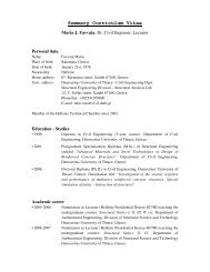
In order to demonstrate the separation quality of the
algorithm, we constructed a synthetic mixture of two sources.
The mixtures contained delayed components of 25ms maximum,
as well as the direct path signals. The fixed-point algorithm
managed to separate the input sources quite well. We can see the
spectrograms of the original and separated sources in figures 1,2.
Figure 1. (a) Spectrogram of the original source and (b)
spectrogram of the separated source using the fixed-point
algorithm
The separation quality is quite good, and almost all the
frequency components of the original sources are preserved in
the separated outputs. We can clearly see that there is no
permutation problem visible or audible in these spectrograms.
21-24 October 2001, New Paltz, New York W2001-3

The permutation problem is well described in [4], where it is
shown that although some algorithms perform reasonable
separation for every frequency bin, we can see source
permutation changes at certain frequencies. As a result, each
source estimate contains large proportions of both sources which
are both audible.
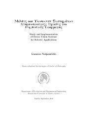
Another test was to apply the algorithm to audio signals.
We used some real data available from [9] of somebody
counting and some music playing simultaneously in a room. The
results were equally satisfactory as with the previous
experiments.
Figure 2. (a) Spectrogram of the original source and (b)
spectrogram of the separated source using the fixed-point
algorithm
Finally, we have also recorded two guitars playing triads in
harmony and created a synthetic mixture using the mixing
function, used in the previous example. This separation
experiment is quite demanding, as there is strong correlation
between the two sources, and it is even difficult for the human
ear to separate them. Applying the fixed-point algorithm, we get
quite promising results. Although there is some audible crosstalk,
the algorithm provides reasonable separation of the two
sources. These results are quite encouraging for instrument
separation from audio recordings.
W2001-4
5. CONCLUSIONS
In this study, we have shown that we can improve the
performance and the stability of maximum likelihood ICA
methods, by introducing a pre-scaling of the time-frequency
input data before processing.
Moreover, we have introduced a new fixed-point algorithm
for frequency domain source separation of convolved mixtures.
The algorithm proved to be more stable and faster compared to
former maximum likelihood approaches, as it is based on a
second order optimization method. The quality of the separation
is quite good, although there is a small amount of cross-talk.
Furthermore, the likelihood ratio jump solution introduced
in [4] proved to be able to solve the permutation problem, even
in a fixed-point framework. However, this likelihood test
becomes more complicated for more than two sources.
In future, we hope to formulate this likelihood ratio jump
test for more sources. Moreover, we hope to improve the
performance and speed of this fixed-point solution as well as
introduce more sophisticated time-frequency models.
6. REFERENCES
[1] Smaragdis P., "Efficient Blind Separation of Convolved
Sound Mixtures", IEEE ASSP Workshop on Applications of
Signal Processing to Audio and Acoustics. New Paltz NY,
October 1997.
[2] Smaragdis P., "Blind Separation of convolved mixtures in
the frequency domain", International Workshop on
Independence & Artificial Neural Networks University of
La Laguna, Tenerife, Spain, February 9 - 10, 1998.
[3] Smaragdis P., "Information Theoretic Approaches to Source
Separation", May 1997, Masters Thesis, MIT Media Lab
[4] Davies M., "Audio Source Separation", Mathematics in
Signal Processing V, 2000.
[5] Amari S., Cichocki A., Yang H. H., "A new learning
algorithm for blind source separation", Advances in Neural
Information Processing Systems, pp. 757-763, MIT Pres,
Cambridge MA, 1996.
[6] Hyvarinen A., "Survey on Independent Component
Analysis”, Neural Computing Surveys 2:94--128, 1999
[7] Hyvärinen A., Oja E., "A Fast Fixed-Point Algorithm for
Independent Component Analysis", Neural Computation,
9(7):1483-1492, 1997.
[8] Hyvarinen A., "The Fixed-point Algorithm and maximum
likelihood estimation for Independent Component Analysis",
Neural Processing Letters, 10(1):1-5.
[9] http://www.cnl.salk.edu/~tewon/ica_cnl.html
[10] Bingham E., Hyvarinen A., " A fast fixed-point algorithm
for independent component analysis of complex-valued
signals", Int. J. of Neural Systems, 10(1):1-8, 2000.
[11] Schobben D., Torkkola K., Smaragdis P., "Evaluation of
blind signal separation methods", Proceedings of the
Workshop on Independent Component Analysis and Blind
Signal Separation, Aussois, France, January 11-15 1999.
2001 IEEE Workshop on Applications of Signal Processing to Audio and Acoustics