Multiple_Integrals.mth: Solving problems of Multiple Integrals with ...
Multiple_Integrals.mth: Solving problems of Multiple Integrals with ...
Multiple_Integrals.mth: Solving problems of Multiple Integrals with ...

Create successful ePaper yourself
Turn your PDF publications into a flip-book with our unique Google optimized e-Paper software.
Dresden International Symposium on Technology and its<br />
Integration into Mathematics Education 2006<br />
DES-TIME 2006<br />
DRESDEN 20th-23th July 2006<br />
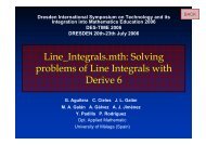
<strong>Multiple</strong>_<strong>Integrals</strong>.<strong>mth</strong>: <strong>Solving</strong><br />
<strong>problems</strong> <strong>of</strong> <strong>Multiple</strong> <strong>Integrals</strong><br />
<strong>with</strong> Derive 6<br />
G. Aguilera C. Cielos J. L. Galán<br />
M. A. Galán A. Gálvez A. J. Jiménez<br />
Y. Padilla P. Rodríguez<br />
Dpt. Applied Mathematic<br />
University <strong>of</strong> Málaga (Spain)
Introduction.<br />
Our experience:<br />
– S<strong>of</strong>tware to use.<br />
Index<br />
– Innovative aspect <strong>of</strong> the experience.<br />
<strong>Multiple</strong> <strong>Integrals</strong> <strong>with</strong> Derive.<br />
Final conclusions.
Introduction<br />
In most cases, the use <strong>of</strong> CAS is reduced<br />
to using computers as powerful highperformance<br />
calculators.<br />
It is therefore necessary to change the<br />
way people think about information<br />
technologies in order to optimise the<br />
opportunities they <strong>of</strong>fer and try to<br />
encourage mathematical creativity among<br />
students.
Introduction<br />
Math teachers that use CAS have to change the<br />
traditional uses given to these tools.<br />
It is a mistake to use CAS in teaching as simple<br />
problem-solving machines.<br />
They should be used in ways that maximize the<br />
opportunities that these technologies <strong>of</strong>fer:<br />
positively affecting student learning, significantly<br />
increasing opportunities for experimentation and<br />
allowing students to construct their own<br />
mathematical knowledge.
Introduction<br />
Math teachers must first set out a series<br />
<strong>of</strong> appropriate activities.<br />
The use <strong>of</strong> CAS in Mathematics has not<br />
reached optimum conditions. Mostly are<br />
blackbox (showing the result in one step<br />
<strong>with</strong>out teaching students how to get<br />
there) and should be whitebox (showing<br />
intermediate steps).
Combining programming<br />
and CAS<br />
When students program, they must read,<br />
construct and refine strategies, modify<br />
previously written programs and lastly, use the<br />
programs to solve <strong>problems</strong>. This makes them<br />
the protagonists <strong>of</strong> their own learning.<br />
The most appropriate approach involves using<br />
programming and CAS together to allow<br />
students to create the specific necessary<br />
functions that will allow them to solve the<br />
<strong>problems</strong> involved in the subject matter under<br />
study.
Our experience<br />
Our experience over the past ten years<br />
has consisted mainly <strong>of</strong> continuously<br />
carrying out practical experiments in the<br />
computer laboratory in Mathematics<br />
courses for the degrees <strong>of</strong> Technical<br />
Industrial Engineering and Technical<br />
Telecommunications Engineering at the<br />
University <strong>of</strong> Málaga.
S<strong>of</strong>tware to use<br />
Among the great amount <strong>of</strong> mathematical<br />
s<strong>of</strong>tware, we have chosen the program<br />
Derive for several reasons:<br />
1. Derive is easier to use than other mathematical<br />
programs as it operates <strong>with</strong> a very simple syntax.<br />
2. The student is capable <strong>of</strong> starting to solve<br />
<strong>problems</strong> by using the program in a short period <strong>of</strong><br />
time, since basic functions and operations are<br />
available in several menus<br />
3. It needs few requirements, <strong>with</strong> regard either to<br />
memory and physical space, when it comes to<br />
installing it
Innovative aspect <strong>of</strong> our<br />
experience<br />
The main innovative aspect <strong>of</strong> these<br />
experiences is that the students have an<br />
active role in the sense they should<br />
elaborate themselves utility files to solve<br />
the typical <strong>problems</strong> for the different<br />
subjects. This fact implies that the<br />
students need to deal <strong>with</strong> programming<br />
in Derive, to understand the subject and<br />
to know how to solve typical <strong>problems</strong>.
Innovative aspect <strong>of</strong> our<br />
experience<br />
The fact that the students themselves<br />
are making the programs and including<br />
all <strong>of</strong> their arguments has a positive<br />
influence on their ability to subsequently<br />
apply them to solve specific exercises.<br />
So, <strong>with</strong> this kind <strong>of</strong> activities CAS<br />
encourages active learning, greater<br />
comprehension <strong>of</strong> subject matter and<br />
mathematical creativity among students.
Double integrals:<br />
– In Cartesian coordinates.<br />
– In polar coordinates.<br />
Triple integrals:<br />
Contents <strong>of</strong><br />
<strong>Multiple</strong>_<strong>Integrals</strong>.<strong>mth</strong><br />
– In Cartesian coordinates<br />
– In cylindrical coordinates.<br />
– In spherical coordinates.<br />
Applications <strong>of</strong> <strong>Multiple</strong> <strong>Integrals</strong>
Final Conclusions<br />
Our accumulated experience reveals that<br />
CAS are computer tools which are easy to<br />
use and useful in Mathematics courses for<br />
Engineering.<br />
The traditional uses given to CAS in the<br />
teaching <strong>of</strong> Mathematics for Engineering must<br />
be changed to maximize the opportunities<br />
<strong>of</strong>fered by CAS technologies. Optimal use<br />
should be aimed at improving student<br />
motivation, autonomy and achieving<br />
participatory and student-centred learning.
Final Conclusions<br />
One powerful idea involves combining CAS<br />
resources <strong>with</strong> the flexibility <strong>of</strong> a programming<br />
language.<br />
There exists reasonable evidence to show<br />
that making programs <strong>with</strong> Derive facilitates<br />
learning and improves student motivation.<br />
Although it would be desirable to do so, it is<br />
not necessary to substantially modify the<br />
traditional program <strong>of</strong> studies <strong>of</strong> Math courses<br />
for Engineering to introduce the innovation <strong>of</strong><br />
having students make their own programs<br />
<strong>with</strong> Derive.
Dresden International Symposium on Technology and its<br />
Integration into Mathematics Education 2006<br />
DES-TIME 2006<br />
DRESDEN 20th-23th July 2006<br />
<strong>Multiple</strong>_<strong>Integrals</strong>.<strong>mth</strong>: <strong>Solving</strong><br />
<strong>problems</strong> <strong>of</strong> <strong>Multiple</strong> <strong>Integrals</strong><br />
<strong>with</strong> Derive 6<br />
G. Aguilera C. Cielos J. L. Galán<br />
M. A. Galán A. Gálvez A. J. Jiménez<br />
Y. Padilla P. Rodríguez<br />
Dpt. Applied Mathematic<br />
University <strong>of</strong> Málaga (Spain)
________________________________________________________<br />
<strong>Multiple</strong>_<strong>Integrals</strong>.dfw:<br />
<strong>Multiple</strong> integrals and its applications<br />
July, 2006<br />
José Luis Galán García<br />
Pedro Rodríguez Cielos<br />
M. Angeles Galán García<br />
Yolanda Padilla Domínguez<br />
Department <strong>of</strong> Applied Mathematic<br />
University <strong>of</strong> Málaga<br />
http://www.satd.uma.es/matap/<br />
________________________________________________________<br />
The following functions have been developed in this utility/demo dfw file to deal <strong>with</strong> multiple integrals and some <strong>of</strong><br />
their applications:<br />
• Doble and triple integrals. Green-Riemann's theorem<br />
o double(f,var1,lim1,lim2,var2,lim3,lim4) to calculate the double integral <strong>of</strong> f <strong>with</strong> the<br />
corresponding variables and limits <strong>of</strong> integration using<br />
cartesian coordinates.<br />
o doublepolar(f,º,º1,º2,²,²1,²2) to calculate the double integral <strong>of</strong> f <strong>with</strong> the<br />
corresponding variables and limits <strong>of</strong> integration using<br />
polar coordinates.<br />
o triple(f,var1,lim1,lim2,var2,lim3,lim4,var3,lim5,lim6) to calculate the triple integral <strong>of</strong> f <strong>with</strong> the<br />
corresponding variables and limits <strong>of</strong> integration using<br />
cartesian coordinates.<br />
o triplecylindrical(f,z,z1,z2,º,º1,º2,²,²1,²2) to calculate the triple integral <strong>of</strong> f <strong>with</strong> the corresponding<br />
variables and limits <strong>of</strong> integration using cylindrical<br />
coordinates.<br />
o triplespherical(f,º,º1,º2,²,²1,²2,¾,¾1,¾2) to calculate the triple integral <strong>of</strong> f <strong>with</strong> the corresponding<br />
variables and limits <strong>of</strong> integration using spherical<br />
coordinates.<br />
• Applications: Green-Riemann's theorem. Surface integrals. Gauss' theorem<br />
o linegreenriemann(P,Q,y,y1,y2,x,x1,x2) to calculate the line integral <strong>of</strong> the field (P,Q) along the<br />
curve limit <strong>of</strong> the region bounded by the corresponding<br />
variables and limits <strong>of</strong> integration in cartesian coordinates,<br />
using Green-Riemann's theorem.
o linegreenriemannpolar(P,Q,º,º1,º2,²,²1,²2) to calculate the line integral <strong>of</strong> the field (P,Q) along the<br />
curve limit <strong>of</strong> the region bounded by the corresponding<br />
variables and limits <strong>of</strong> integration in polar coordinates,<br />
using Green-Riemann's theorem.<br />
o surfacearearxy(S,y,y1,y2,x,x1,x2) to calculate the area <strong>of</strong> the surface S ≡ z=z(x,y) <strong>with</strong> the limits <strong>of</strong><br />
integration in Rxy.<br />
o surfacearearxz(S,x,x1,x2,z,z1,z2) to calculate the area <strong>of</strong> the surface S ≡ y=y(x,z) <strong>with</strong> the limits <strong>of</strong><br />
integration in Rxz.<br />
o surfacearearyz(S,z,z1,z2,y,y1,y2) to calculate the area <strong>of</strong> the surface S ≡ x=x(y,z) <strong>with</strong> the limits <strong>of</strong><br />
integration in Ryz.<br />
o surfacearearxypolar(S,º,º1,º2,²,²1,²2) to calculate the area <strong>of</strong> the surface S ≡ z=z(x,y) <strong>with</strong> the limits <strong>of</strong><br />
integration in Rxy in polar coordinates.<br />
o surfacearearxzpolar(S,º,º1,º2,²,²1,²2) to calculate the area <strong>of</strong> the surface S ≡ y=y(x,z) <strong>with</strong> the limits <strong>of</strong><br />
integration in Rxz in polar coordinates.<br />
o surfacearearyzpolar(S,º,º1,º2,²,²1,²2) to calculate the area <strong>of</strong> the surface S ≡ x=x(y,z) <strong>with</strong> the limits <strong>of</strong><br />
integration in Ryz in polar coordinates.<br />
o surfacerxy(f,S,y,y1,y2,x,x1,x2) to integrate the function f over the surface S ≡ z=z(x,y) <strong>with</strong> the<br />
limits <strong>of</strong> integration in Rxy.<br />
o surfacerxz(f,S,x,x1,x2,z,z1,z2) to integrate the function f over the surface S ≡ y=y(x,z) <strong>with</strong> the<br />
limits <strong>of</strong> integration in Rxz.<br />
o surfaceryz(f,S,z,z1,z2,y,y1,y2) to integrate the function f over the surface S ≡ x=x(y,z) <strong>with</strong> the<br />
limits <strong>of</strong> integration in Ryz.<br />
o surfacerxypolar(f,S,º,º1,º2,²,²1,²2) to integrate the function f over the surface S ≡ z=z(x,y) <strong>with</strong> the<br />
limits <strong>of</strong> integration in Rxy in polar coordinates.<br />
o surfacerxzpolar(f,S,º,º1,º2,²,²1,²2) to integrate the function f over the surface S ≡ y=y(x,z) <strong>with</strong> the<br />
limits <strong>of</strong> integration in Rxz in polar coordinates.<br />
o surfaceryzpolar(f,S,º,º1,º2,²,²1,²2) to integrate the function f over the surface S ≡ x=x(y,z) <strong>with</strong> the<br />
limits <strong>of</strong> integration in Ryz in polar coordinates.<br />
o unitnormalvector(F) to calculate an unit normal vector <strong>of</strong> the surface S ≡ F(x,y,z)=0.<br />
o fluxrxy(P,Q,R,S,y,y1,y2,x,x1,x2) to calculate the flux <strong>of</strong> (P,Q,R) over the surface S ≡ z=z(x,y)<br />
<strong>with</strong> the limits <strong>of</strong> integration in Rxy.<br />
o fluxrxz(P,Q,R,S,x,x1,x2,z,z1,z2) to calculate the flux <strong>of</strong> (P,Q,R) over the surface S ≡ y=y(x,z)<br />
<strong>with</strong> the limits <strong>of</strong> integration in Rxz.<br />
o fluxryz(P,Q,R,S,z,z1,z2,y,y1,y2) to calculate the flux <strong>of</strong> (P,Q,R) over the surface S ≡ x=x(y,z)<br />
<strong>with</strong> the limits <strong>of</strong> integration in Ryz.<br />
o fluxrxypolar(P,Q,R,S,º,º1,º2,²,²1,²2) to calculate the flux <strong>of</strong> (P,Q,R) over the surface S ≡ z=z(x,y)<br />
<strong>with</strong> the limits <strong>of</strong> integration in Rxy in polar coordinates.<br />
o fluxrxzpolar(P,Q,R,S,º,º1,º2,²,²1,²2) to calculate the flux <strong>of</strong> (P,Q,R) over the surface S ≡ y=y(x,z)<br />
<strong>with</strong> the limits <strong>of</strong> integration in Rxz in polar coordinates.<br />
o fluxryzpolar(P,Q,R,S,º,º1,º2,²,²1,²2) to calculate the flux <strong>of</strong> (P,Q,R) over the surface S ≡ x=x(y,z)<br />
<strong>with</strong> the limits <strong>of</strong> integration in Ryz in polar coordinates.<br />
o fluxgauss(P,Q,R,z,z1,z2,y,y1,y2,x,x1,x2) to calculate the flux <strong>of</strong> (P,Q,R) over the surface S limit <strong>of</strong> the<br />
solid which limits <strong>of</strong> integration are given in cartesian<br />
coordinates.<br />
o fluxgausscylindrical(P,Q,R,z,z1,z2,º,º1,º2,²,²1,²2) to calculate the flux <strong>of</strong> (P,Q,R) over the surface S<br />
limit <strong>of</strong> the solid which limits <strong>of</strong> integration are<br />
given in cylindrical coordinates.
o fluxgaussspherical(P,Q,R,º,º1,º2,²,²1,²2,¾,¾1,¾2) to calculate the flux <strong>of</strong> (P,Q,R) over the surface S<br />
limit <strong>of</strong> the solid which limits <strong>of</strong> integration are<br />
given in spherical coordinates.<br />
MULTIPLE INTEGRALS. GREEN-RIEMANN'S THEOREM<br />
_____________________________________________________<br />
• Double integration in cartesian coordinates<br />
o Syntax: DOUBLE(function,var1,lim1,lim2,var2,lim3,lim4)<br />
o Example: double(xy,y,0,x+1,x,0,2) to integrate the function f(x,y) = xy<br />
in the region bounded by<br />
x = 2 , y = x+1 , y = 0 and x = 0<br />
#1: DOUBLE(x·y, y, 0, x + 1, x, 0, 2)<br />
17<br />
#2: ⎯⎯<br />
3<br />
• Double integration in polar coordinates<br />
o Syntax: DOUBLEPOLAR(function,r,r1,r2,theta,theta1,theta2)<br />
o Example: doublepolar(x^2y^2/(x^2+y^2),r,0,1,theta,0,pi)<br />
to integrate the function f(x,y) = x 2 y 2 /(x 2 + y 2 ) in the region<br />
bounded by x 2 +y 2 = 1 <strong>with</strong> y ’ 0<br />
⎛ 2 2 ⎞<br />
⎜ x ·y ⎟<br />
#3: DOUBLEPOLAR⎜⎯⎯⎯⎯⎯⎯⎯, r, 0, 1, θ, 0, π⎟<br />
⎜ 2 2 ⎟<br />
⎝ x + y ⎠<br />
π<br />
#4: ⎯⎯<br />
32
• Triple integration in cartesian coordinates<br />
o Syntax: TRIPLE(function,var1,lim1,lim2,var2,lim3,lim4,var3,lim5,lim6)<br />
o Example: triple(x+yz,z,0,5-x-y,y,0,5-x,x,0,5) to integrate the function<br />
f(x,y,z) = x+yz in the solid<br />
bounded by x+y+z = 5 ,<br />
x = 0 , y = 0 and z = 0<br />
#5: TRIPLE(x + y·z, z, 0, 5 - x - y, y, 0, 5 - x, x, 0, 5)<br />
625<br />
#6: ⎯⎯⎯<br />
12<br />
• Triple integration in cylindrical coordinates<br />
o Syntax: TRIPLECYLINDRICAL(function,z,z1,z2,r,r1,r2,theta,theta1,theta2)<br />
o Example: triplecylindrical(sqrt(x^2+y^2),z,r,1,r,0,1,theta,0,2pi)<br />
to integrate the function f(x,y,z) = ‹(x 2 +y 2 ) in the solid<br />
bounded by z = 0 , z = 1 and z 2 = x 2 +y 2<br />
2 2<br />
#7: TRIPLECYLINDRICAL(√(x + y ), z, r, 1, r, 0, 1, θ, 0, 2·π)<br />
π<br />
#8: ⎯<br />
6<br />
• Triple integration in spherical coordinates<br />
o Syntax: TRIPLESPHERICAL(function,r,r1,r2,theta,theta1,theta2,phi,phi1,phi2)<br />
o Example: triplespherical(x+y+z,r,0,2,theta,0,2pi,phi,0,pi/2)<br />
to integrate the function f(x,y,z) = x+y+z in the solid<br />
bounded by x 2 + y 2 + z 2 = 4 <strong>with</strong> z ’ 0<br />
⎛ π ⎞<br />
#9: TRIPLESPHERICAL⎜x + y + z, r, 0, 2, θ, 0, 2·π, α, 0, ⎯⎟<br />
⎝ 2 ⎠
#10: 4·π<br />
APPLICATIONS OF MULTIPLE INTEGRLAS<br />
_________________________________________<br />
• Green-Riemann's theorem in cartesian coordinates<br />
o Syntax: LINEGREENRIEMANN(comp1,comp2,y,y1,y2,x,x1,x2)<br />
o Example: linegreenriemann(y^2,x,y,0,3,x,0,3) to calculate the line integrate <strong>of</strong><br />
(y 2 ,x) along the square <strong>of</strong> vertices<br />
(0,0) , (3,0) , (3,3) , (0,3) using<br />
Green-Riemann's theorem<br />
2<br />
#11: LINEGREENRIEMANN(y , x, y, 0, 3, x, 0, 3)<br />
#12: -18<br />
• Green-Riemann's theorem in polar coordinates<br />
o Syntax: LINEGREENRIEMANNPOLAR(comp1,comp2,r,r1,r2,theta,theta1,theta2)<br />
o Example: linegreenriemannpolar(y^2,x,r,0,5,theta,0,2pi)<br />
to calculate the line integrate <strong>of</strong> (y 2 ,x) along the circumference<br />
x 2 +y 2 =25 using Green-Riemann's theorem<br />
2<br />
#13: LINEGREENRIEMANNPOLAR(y , x, r, 0, 5, θ, 0, 2·π)<br />
#14: 25·π<br />
• Surface area in polar coordinates<br />
o Syntax: SURFACEAREARXYPOLAR(z surface,r,r1,r2,theta,theta1,theta2)
o Example: surfacearearxypolar(sqrt(x^2+y^2),r,0,1,theta,0,2pi)<br />
to calculate the area <strong>of</strong> the part <strong>of</strong> the surface z 2 = x 2 + y 2<br />
inside <strong>of</strong> z = 2 - x 2 - y 2 <strong>with</strong> z ’ 0<br />
2 2<br />
#15: SURFACEAREARXYPOLAR(√(x + y ), r, 0, 1, θ, 0, 2·π)<br />
#16: √2·π<br />
• Unit normal vector to an implicit surface<br />
o Syntax: UNITNORMALVECTOR(implicit surface)<br />
o Example: unitnormalvector(x^2+y^2+z^2-4) to find an unit normal<br />
vector to x 2 + y 2 + z 2 = 4<br />
2 2 2<br />
#17: UNITNORMALVECTOR(x + y + z - 4)<br />
⎡ x y z ⎤<br />
⎢⎯⎯⎯⎯⎯⎯⎯⎯⎯⎯⎯⎯⎯⎯⎯, ⎯⎯⎯⎯⎯⎯⎯⎯⎯⎯⎯⎯⎯⎯⎯, ⎯⎯⎯⎯⎯⎯⎯⎯⎯⎯⎯⎯⎯⎯⎯⎥<br />
#18: ⎢ 2 2 2 2 2 2 2 2 2 ⎥<br />
⎣ √(x + y + z ) √(x + y + z ) √(x + y + z ) ⎦<br />
• Flux <strong>of</strong> a vector field. Double integral in polar coordinates<br />
o Syntax: FLUXRXYPOLAR(comp1,comp2,comp3,zsurface,r,r1,r2,theta,theta1,theta2)<br />
o Example: fluxrxypolar(x,2y,x+z,x^2+y^2,r,0,4,theta,0,2pi)<br />
to calculate the flux <strong>of</strong> (x,2y,x+z) over the part <strong>of</strong> the surface<br />
<strong>of</strong> the paraboloid z = x 2 + y 2 for which 0 ≤ z ≤ 16<br />
2 2<br />
#19: FLUXRXYPOLAR(x, 2·y, x + z, x + y , r, 0, 4, θ, 0, 2·π)<br />
#20: - 256·π<br />
• Gauss' theorem. Triple integral in cartesian coordinates<br />
o Syntax: FLUXGAUSS(c1,c2,c3,z,z1,z2,y,y1,y2,x,x1,x2)
o Example: fluxgauss(x,y,z,z,0,1,y,0,1,x,0,1) to calculate the flux <strong>of</strong> (x,y,z)<br />
over the closed surface<br />
bounded by the unit cube<br />
#21: FLUXGAUSS(x, y, z, z, 0, 1, y, 0, 1, x, 0, 1)<br />
#22: 3<br />
• Gauss' theorem. Triple integral in cylindrical coordinates<br />
o Syntax: FLUXGAUSSCYLINDRICAL(c1,c2,c3,z,z1,z2,r,r1,r2,theta,theta1,theta2)<br />
o Example: fluxgausscylindrical(x,2y,3z,z,r,2,r,0,2,theta,0,2pi)<br />
to calculate the flux <strong>of</strong> (x,2y,3z) over the closed surface<br />
bounded by the cone z 2 = x 2 + y 2 and the planes z = 0, z = 2<br />
#23: FLUXGAUSSCYLINDRICAL(x, 2·y, 3·z, z, r, 2, r, 0, 2, θ, 0, 2·π)<br />
#24: 16·π<br />
• Gauss' theorem. Triple integral in spherical coordinates<br />
o Syntax: FLUXGAUSSSPHERICAL(c1,c2,c3,r,r1,r2,theta,theta1,theta2,phi,phi1,phi2)<br />
o Example: fluxgaussspherical(x^2z+x,y,z,r,0,1,theta,0,2pi,phi,0,pi/2)<br />
to calculate the flux <strong>of</strong> (x 2 z+x,y,z) over the closed surface bounded<br />
by the semi-sphere x 2 + y 2 + z 2 = 1 and z = 0 <strong>with</strong> z ’ 0<br />
⎛ 2 π ⎞<br />
#25: FLUXGAUSSSPHERICAL⎜x ·z + x, y, z, r, 0, 1, θ, 0, 2·π, φ, 0, ⎯⎟<br />
⎝ 2 ⎠<br />
#26: 2·π
Cartesian coordinates<br />
#1: [u1 ≔, u2 ≔, v1 ≔, v2 ≔, w1 ≔, w2 ≔]<br />
#2: f<br />
u2<br />
#3: ∫ f du<br />
u1<br />
v2<br />
⌠ u2<br />
#4: ⎮ ∫ f du dv<br />
⌡ u1<br />
v1<br />
Double <strong>Integrals</strong><br />
v2<br />
⌠ u2<br />
#5: double(f, u, u1, u2, v, v1, v2) ≔ ⎮ ∫ f du dv<br />
⌡ u1<br />
v1<br />
Polar coordinates<br />
#6: SUBST(f, [x, y], [ρ·COS(θ), ρ·SIN(θ)])<br />
#7: ρ·SUBST(f, [x, y], [ρ·COS(θ), ρ·SIN(θ)])<br />
#8: doublepolar(f, u, u1, u2, v, v1, v2) ≔ double(ρ·SUBST(f, [x, y],<br />
[ρ·COS(θ), ρ·SIN(θ)]), u, u1, u2, v, v1, v2)
Cartesian coordinates<br />
#9: f<br />
u2<br />
#10: ∫ f du<br />
u1<br />
v2<br />
⌠ u2<br />
#11: ⎮ ∫ f du dv<br />
⌡ u1<br />
v1<br />
w2<br />
⌠ v2<br />
⎮ ⌠ u2<br />
#12: ⎮ ⎮ ∫ f du dv dw<br />
⎮ ⌡ u1<br />
⌡ v1<br />
w1<br />
Triple <strong>Integrals</strong><br />
w2<br />
⌠ v2<br />
⎮ ⌠ u2<br />
#13: triple(f, u, u1, u2, v, v1, v2, w, w1, w2) ≔ ⎮ ⎮ ∫ f du dv dw<br />
⎮ ⌡ u1<br />
⌡ v1<br />
w1<br />
Cylindrical coordinates<br />
#14: SUBST(f, [x, y, z], [ρ·COS(θ), ρ·SIN(θ), z])<br />
#15: ρ·SUBST(f, [x, y, z], [ρ·COS(θ), ρ·SIN(θ), z])<br />
#16: triplecylindrical(f, u, u1, u2, v, v1, v2, w, w1, w2) ≔<br />
triple(ρ·SUBST(f, [x, y, z], [ρ·COS(θ), ρ·SIN(θ), z]), u, u1,<br />
u2, v, v1, v2, w, w1, w2)
Spherical coordinates<br />
#17: SUBST(f, [x, y, z], [ρ·COS(φ)·COS(θ), ρ·COS(φ)·SIN(θ), ρ·SIN(φ)])<br />
2<br />
#18: ρ ·COS(φ)·SUBST(f, [x, y, z], [ρ·COS(φ)·COS(θ), ρ·COS(φ)·SIN(θ),<br />
ρ·SIN(φ)])<br />
#19: triplespherical(f, u, u1, u2, v, v1, v2, w, w1, w2) ≔<br />
2<br />
triple(ρ ·COS(φ)·SUBST(f, [x, y, z], [ρ·COS(φ)·COS(θ),<br />
ρ·COS(φ)·SIN(θ), ρ·SIN(φ)]), u, u1, u2, v, v1, v2, w, w1, w2)<br />
Exercise 1<br />
Exercises<br />
Compute the area <strong>of</strong> the circle x^2+y^2 ≤ 16 using Cartesian<br />
and polar coordinates.<br />
2 2<br />
#20: x + y ≤ 16
2 2<br />
#21: double(1, y, - √(16 - x ), √(16 - x ), x, -4, 4)<br />
#22: 16·π<br />
2 2<br />
#23: SUBST(x + y ≤ 16, [x, y], [ρ·COS(θ), ρ·SIN(θ)])<br />
#24: -4 ≤ ρ ≤ 4<br />
#25: doublepolar(1, ρ, 0, 4, θ, 0, 2·π)<br />
#26: 16·π<br />
Exercise 2<br />
Calculate the volume <strong>of</strong> the solid bounded below by the cone<br />
z = √(x^2+y^2) and above by the sphere x^2+y^2+z^2 = 2<br />
using Cartesian, cylindrical and spherical coordinates.<br />
2 2<br />
#27: z = √(x + y )<br />
2 2<br />
#28: z = √(2 - x - y )<br />
2 2 2 2 2<br />
#29: triple(1, z, √(x + y ), √(2 - x - y ), y, - √(1 - x ), √(1 -<br />
2<br />
x ), x, -1, 1)
#30: The computer cannot compute this calculation in Cartesian<br />
coordinates.<br />
2 2<br />
#31: z = √((ρ·COS(θ)) + (ρ·SIN(θ)) )<br />
#32: z = ⎮ρ⎮<br />
2 2<br />
#33: z = √(2 - (ρ·COS(θ)) - (ρ·SIN(θ)) )<br />
2<br />
#34: z = √(2 - ρ )<br />
2<br />
#35: triplecylindrical(1, z, ρ, √(2 - ρ ), ρ, 0, 1, θ, 0, 2·π)<br />
⎛ 4·√2 4 ⎞<br />
#36: π·⎜⎯⎯⎯⎯ - ⎯⎟<br />
⎝ 3 3 ⎠<br />
2 2 2<br />
#37: z = x + y<br />
2 2 2<br />
#38: (ρ·SIN(φ)) = (ρ·COS(φ)·COS(θ)) + (ρ·COS(φ)·SIN(θ))<br />
2 2 2 2<br />
#39: ρ ·SIN(φ) = ρ ·COS(φ)<br />
π<br />
#40: φ = ⎯<br />
4<br />
2 2 2<br />
#41: x + y + z = 2<br />
2 2 2<br />
#42: (ρ·COS(φ)·COS(θ)) + (ρ·COS(φ)·SIN(θ)) + (ρ·SIN(φ)) = 2<br />
2<br />
#43: ρ = 2<br />
⎛ π π ⎞<br />
#44: triplespherical⎜1, ρ, 0, √2, θ, 0, 2·π, φ, ⎯, ⎯⎟<br />
⎝ 4 2 ⎠<br />
⎛ 4·√2 4 ⎞<br />
#45: π·⎜⎯⎯⎯⎯ - ⎯⎟<br />
⎝ 3 3 ⎠