Download (20MB) - Repository@Napier
Download (20MB) - Repository@Napier
Download (20MB) - Repository@Napier

You also want an ePaper? Increase the reach of your titles
YUMPU automatically turns print PDFs into web optimized ePapers that Google loves.
AN INVESTIGATION INTO THE PROCESSES RESPONSIBLE<br />
FOR THE GENERATION OF THE SPATIAL PATTERN OF<br />
THE SPIONID POLYCHAETE PYGOSPIO ELEGANS<br />
CLAPAREDE<br />
STEFAN GEORGE BOLAM<br />
A thesis submitted in partial fulfilment of the requirements of Napier<br />
University for the degree of Doctor of Philosophy.<br />
July 1999
I declare that this thesis was written by me and that the work contained herein is my<br />
own.<br />
S-6t9,- •<br />
Stefan G. Bolam<br />
ii
ABSTRACT<br />
The spionid polychaete Pygospio elegans Claparede (1863) is a small, tube-building<br />
opportunist. On the intertidal sandflat Drum Sands, Firth of Forth, Scotland, this<br />
species is numerically dominant and forms areas of increased density or 'patches'.<br />
Grid surveys, together with mapping and spatial autocorrelation analysis, revealed that<br />
these patches were areas of statistically significant higher numbers of P. elegans<br />
compared with surrounding areas where this species was present in very low numbers.<br />
These patches, 1-1.5m2, could be seen as areas of smooth, raised sediment within an<br />
otherwise wave-rippled sandflat. The majority of the other macrobenthic invertebrate<br />
species also exhibited small- or meso-scale patchiness, but none of these patches were<br />
spatially coincident with those of P. elegans.<br />
Although life history characteristics and disturbance have previously been postulated as<br />
being responsible for the generation of spionid patches, these have never been<br />
explicitly tested. The P. elegans population on Drum Sands was studied with respect<br />
to its population structure and reproductive biology and its response to macroalgal mat<br />
establishment and sediment disturbance. The possible role of these in the formation of<br />
small-scale patches of P. elegans are discussed.<br />
The P. elegans population on Drum Sands displayed reproductive activity for the<br />
majority of the year although intense larval recruitment was confined to two acute<br />
periods, April/May and November/December. P. elegans reproduced exclusively via<br />
planktotrophic larvae: no evidence of asexual proliferation or benthic larval production<br />
was found. This life history provides a large larval availability for patch formation.<br />
The role of macroalgal mat establishment in structuring the spatial distribution of P.<br />
elegans was investigated by a controlled, weed-implantation experiment and a<br />
comparative survey. Implanted Enteromorpha prolifera and naturally establishing<br />
Vaucheria subsimplex caused underlying sediments to have increased silt/clay<br />
fractions, increased organic and water contents and increased sorting coefficients and
medium grain size. The sediment below these macroalgal mats also became<br />
significantly more reduced. While the communities under E. prolifera mats became<br />
dominated by C. capitata, those under V. subsimplex mats were dominated by P.<br />
elegans.<br />
The effect of sediment disturbance on the faunal communities of Drum Sands was<br />
investigated by studying the initial colonisation of defaunated sediments. P. elegans<br />
numerically dominated the early stages of succession only during periods of high larval<br />
availability, C. capitata dominated at other times. Furthermore, P. elegans larval<br />
recruitment and adult immigration to defaunated sediments within P. elegans patches<br />
were higher compared with non-patch defaunated sediments.<br />
The micro-scale spatial distribution of P. elegans within small-scale patches was<br />
examined. P. elegans was found to be non-randomly distributed throughout the year,<br />
patches formed were commonly less than 3cm2. Correlation analyses implied that<br />
these micro-scale patches may have been generated and maintained by adult-juvenile<br />
interactions and/or sediment heterogeneity.<br />
Small-scale P. elegans patches were found to be distinct ecological areas when<br />
compared with surrounding sediments. Sediment properties and invertebrate<br />
community structure of P. elegans patches were significantly different to those of non-<br />
patch areas. These findings emphasise the ecological importance of patches of tube-<br />
building spionid polychaetes in allowing certain species to occur in habitats where they<br />
would otherwise be unable to survive.<br />
iv
ACKNOWLEDGEMENTS<br />
I am indebted to my supervisors Dr. Teresa Fernandes, Professor Paul Read and Dr.<br />
Dave Raffaelli for their guidance, encouragement and constructive criticism throughout<br />
the course of this study.<br />
I am also very grateful to a number of other people for their help in various aspects of<br />
my study. These are namely Mike Richards for his help in the field, Jill Sales for her<br />
help with statistical analyses, Peter Gibson for helping with faunal identification, Dr.<br />
Richard Ladle for reading through and commenting on the thesis, Marina Marcogni for<br />
her invaluable help with computing and Dagmar Rothaug and Karen Miller for helping<br />
me with fieldwork and sample sorting.<br />
I must also thank a number of other people who I have contacted for specialist advice.<br />
These are Dr. Simon Thrush for his help during the early stages of my research, Dr.<br />
Helgi Gudmundsson and Dr. Torin Morgan for information about Pygospio elegans,<br />
Dr. Pierre Legendre for advice about numerical analyses, Dr. Martin Wilkinson for<br />
identifying my weed samples and Dr. Steve Hull for his advice about macroalgal mat<br />
implantation.<br />
I would like to acknowledge my colleagues in the laboratory, my thanks go to them for<br />
keeping me 'entertained' over the years.<br />
My last thanks, but by no means least, go to Thi for her enduring patience and<br />
understanding over the past couple of years.
t<br />
CONTENTS<br />
DECLARATION. . ii<br />
ABSTRACT . . iii<br />
ACKNOWLEDGEMENTS. . v<br />
CONTENTS . . vi<br />
LIST OF FIGURES . x<br />
LIST OF TABLES .Xiii<br />
CHAPTER 1. INTRODUCTION.<br />
Background . . 1<br />
The present study . 6<br />
Pygospio elegans . 8<br />
The study site . . 10<br />
CHAPTER 2. THE SMALL- TO MESO-SCALE SPATIAL DISTRIBUTION OF . . 15<br />
MARINE BENTHIC INVERTEBRATES ON DRUM SANDS, WITH<br />
PARTICULAR REFERENCE TO PYGOSPIO ELEGANS<br />
Introduction . . 15<br />
Methods . . 19<br />
Scales of spatial variability - Transect survey. . 19<br />
Survey design. . 19<br />
Data analyses . . 21<br />
Pattern analysis - Grid surveys . 22<br />
Survey design . . 22<br />
Data analyses . . 24<br />
Results. . . 27<br />
Scales of spatial variability - Transect survey. . 27<br />
Pattern analysis - Grid surveys . 31<br />
lm survey - spatial patterns . 36<br />
8m survey - spatial patterns . 42<br />
40m surveys - spatial patterns. . 43<br />
Discussion . 51<br />
CHAPTER 3. THE POPULATION STRUCTURE AND REPRODUCTIVE . . 59<br />
BIOLOGY OF PYGOSPIO ELEGANS ON DRUM SANDS.<br />
Introduction .<br />
. 59<br />
Methods . . 63<br />
Survey design . . 63<br />
Data analyses . . 64<br />
vi
Results. . 65<br />
Size distribution of Pygospio elegans. . 65<br />
Sex ratio of Pygospio elegans. . . 70<br />
Reproductive activity of Pygospio elegans . 71<br />
Discussion . . 74<br />
CHAPTER 4. THE EFFECTS OF MACROALGAL COVER ON THE SPATIAL . 83<br />
DISTRIBUTION OF MACROBENTHIC INVERTEBRATES: AN<br />
EXPERIMENTAL STUDY.<br />
Introduction . . 83<br />
Methods . . 87<br />
Study site . . 87<br />
Experimental design . 87<br />
Data analyses . . 91<br />
Results. . 93<br />
Species abundances . 93<br />
Sediment water, organic and silt/clay contents and . 94<br />
granulometry<br />
Redox potentials . . 97<br />
Pygospio elegans size distribution . 99<br />
Algal biomass. . 100<br />
Discussion . . 102<br />
CHAPTER 5. THE EFFECTS OF MACROALGAL COVER ON THE SPATIAL . 109<br />
DISTRIBUTION OF MACROBENTHIC INVERTEBRATES:<br />
A SURVEY APPROACH<br />
Introduction . . 109<br />
Methods . . 111<br />
Survey design . . 111<br />
Data analyses . . 114<br />
Results. . 115<br />
Species abundances . . 115<br />
Sediment water, organic and silt/clay contents and . 118<br />
granulometry<br />
Redox potentials . . . 118<br />
Pygospio elegans size distribution . 121<br />
Algal biomass. . 122<br />
Discussion . . 124<br />
vii
CHAPTER 6. INITIAL COLONISATION OF DISTURBED SEDIMENTS: THE . 131<br />
EFFECTS OF A BIOGENIC SPECIES ON COMMUNITY<br />
ESTABLISHMENT<br />
Introduction . . 131<br />
Methods . 134<br />
Experimental design . 134<br />
Data analyses . . 138<br />
Results. . 141<br />
Univariate analysis of species abundances . 141<br />
Size-frequency analysis . 144<br />
Multivariate analysis of community structure. . 149<br />
Sediment water, organic and silt/clay contents . 162<br />
Redox potentials . 162<br />
Discussion . . 164<br />
CHAPTER 7. THE MICRO-SCALE SPATIAL PATTERNS OF PYGOSPIO . . 172<br />
ELEGANS WITHIN SMALL-SCALE PATCHES AND THE<br />
ROLES OF INTRA- AND INTERSPECIF1C INTERACTIONS<br />
AND ABIOT1C EFFECTS.<br />
Introduction . . 172<br />
Methods . 175<br />
Experimental design . 175<br />
Data analyses . . 177<br />
Results. . 179<br />
Pilot survey . . 179<br />
Transect survey - Micro-scale patterns of P. elegans . . 181<br />
Sediment water, organic and silt/clay contents . 190<br />
Discussion . . 195<br />
CHAPTER 8. THE FAUNAL COMMUNITIES OF PYGOSPIO ELEGANS . . 201<br />
PATCHES.<br />
Introduction . 201<br />
Methods . 204<br />
Results. . 205<br />
Univariate analysis of species abundances . 205<br />
Size-frequency analysis . 208<br />
Multivariate analysis of community structure. . 213<br />
Sediment water, organic and silt/clay contents . 223<br />
Redox potentials . 223<br />
Discussion . . 226<br />
viii
CHAPTER 9. GENERAL DISCUSSION . . 234<br />
REFERENCES . . 244<br />
APPENDICES . . 275<br />
Appendix 1.1 : Species abundances from lm survey, plots 1-64 . . 275<br />
Appendix 1.2 : Species abundances from 8m survey, plots 1-64 . . 278<br />
Appendix 1.3 : Species abundances from 40m survey, plots 1-63 . . 281<br />
Appendix 2 : Species abundances from micro-scale survey . . 284<br />
ix
LIST OF FIGURES<br />
Figure 1.1 Map of the Firth of Forth showing the position of Drum Sands . 12<br />
Figure 1.2 Map of Drum Sands showing the position of the study area . . 13<br />
Figure 1.3 Profile of Drum Sands . . 14<br />
Figure 2.1 Layout of plots for transect survey . 20<br />
Figure 2.2 Sample layout of the 1 m and 8m grid surveys . • 24<br />
Figure 2.3 Species abundances from transect survey (i-vi). • 28<br />
Figure 2.4 Sediment results from transect survey (i-iv) . • 30<br />
Figure 2.5 Contour maps from lm survey (i-vi) . • 39<br />
Figure 2.5 Contour maps from 1 m survey (vii-xii). • 40<br />
Figure 2.6 Correlograms for the fauna and sediments from lm survey (i-ix) • 41<br />
Figure 2.7 Contour maps from 8m survey (i-vi) . • 44<br />
Figure 2.7 Contour maps from 8m survey (vii-xii). . 45<br />
Figure 2.8 Correlograms for the fauna and sediments from 8m survey (i-viii) • 46<br />
Figure 2.9 Contour maps from 40m survey (i-viii). 47<br />
Figure 2.9 Contour maps from 40m survey (ix-xv) . 48<br />
Figure 2.10 Correlograms for the fauna and sediments from the 40m survey . 49<br />
(i-viii)<br />
Figure 2.10 Correlograms for the fauna and sediments from the 40m survey . 50<br />
(ix-xiii)<br />
Figure 3.1 Regression line of 5th setiger width against length for P. elegans . 66<br />
Figure 3.2 Size-frequency histograms of P. elegans (i-ix) . . . 69<br />
Figure 3.3 Mean numbers of male and female P. elegans and sex ratio . . 70<br />
Figure 3.4 Mean number and percentage of female tubes containing embryos . 71<br />
or larvae<br />
Figure 3.5 Size-frequency histograms of P. elegans larvae from adult female<br />
tubes (i-vi)<br />
Figure 4.1 Diagram showing the location of experimental blocks and natural<br />
weed mat establishment during 1996<br />
. 88<br />
Figure 4.2 Experimental layout of weed implantation experiment treatments . 89<br />
Figure 4.3 Mean species abundances for initial, 6 weeks and 20 weeks results<br />
(i-iii)<br />
. 95<br />
Figure 4.4 Sediment water, organic and silt/clay contents and granulometry<br />
results for initial, 6 weeks and 20 weeks samples (i-iii)<br />
. 96<br />
Figure 4.5 Redox potentials for initial, 6, 12 and 20 weeks samples (i-iii) . 98<br />
Figure 4.6 Size-frequency results of P. elegans after 6 and 20 weeks (i-i) . 99<br />
Figure 5.1 Random layout of weed and non-weed plots for weed survey . . 112<br />
Figure 5.2 Faunal results for the weed and non-weed plots after 4 and 20.<br />
weeks (i-i)<br />
. 117<br />
Figure 5.3 % water, organic and silt/clay contents and granulometry results . 119<br />
x<br />
. 73
Figure 5.4<br />
Figure 5.5<br />
Figure 6.1<br />
Figure 6.2<br />
Figure 6.3<br />
Figure 6.4<br />
Figure 6.5<br />
Figure 6.6<br />
Figure 6.7<br />
Figure 6.8<br />
Figure 6.9<br />
Figure 6.10<br />
Figure 6.11<br />
Figure 6.12<br />
Figure 6.13<br />
Figure 6.14<br />
Figure 6.15<br />
Figure 7.1<br />
Figure 7.2<br />
Figure 7.3<br />
Figure 7.4<br />
Figure 7.4<br />
Figure 7.4<br />
Figure 7.5<br />
Figure 7.6<br />
Figure 7.7<br />
Figure 7.8<br />
for weed and non-weed plots after<br />
Redox potential profiles for weed<br />
20 weeks (i-iii)<br />
Size-frequency distributions of P.<br />
4 and 20 weeks (i-i)<br />
and non-weed plots after 4, 8 and . 120<br />
elegans after 4 and 20 weeks (i-i) . 122<br />
Experimental layout of patch and non-patch plots. . . . 135<br />
Mean fauna/ densities after 3 weeks colonisation (i-vii) . . 143<br />
Size-frequency histograms of P. elegans from patch and non-patch . 145<br />
azoic samples (i-vi)<br />
Size-frequency histograms of C. capitata from patch and non-patch . 147<br />
azoic samples (i-vi)<br />
Dendrogram of patch and non-patch replicates for the April . . 152<br />
experiment<br />
Two-dimensional MDS ordination of patch and non-patch replicates . 153<br />
for the April experiment<br />
Dendrogram of patch and non-patch replicates for the August. . 154<br />
experiment<br />
Two-dimensional MDS ordination of patch and non-patch replicates . 155<br />
for the August experiment<br />
Dendrogram of patch and non-patch replicates for the December . 156<br />
experiment<br />
Two-dimensional MDS ordination of patch and non-patch replicates . 157<br />
for the December experiment<br />
Dendrogram of all patch and non-patch replicates . . 159<br />
Two-dimensional MDS ordination of all patch and non-patch. . 160<br />
replicates<br />
Two-dimensional MDS ordination of the average azoic and ambient . 161<br />
communities from patch and non-patch plots<br />
% water content, silt/clay fraction and organic content for patch and . 163<br />
non-patch azoic sediments<br />
Redox potential values for patch and non-patch plots . . 163<br />
Diagram showing the positions of the cores for the pilot survey . 175<br />
Contour map of P. elegans abundance from the pilot survey . . 180<br />
Correlogram of Moran's coefficient against distance class of . . 180<br />
P. elegans density from pilot survey<br />
Density maps of adult P. elegans numbers along transects (i-ix) . 184<br />
Density maps of adult P. elegans numbers along transects (x-xviii) . 185<br />
Density maps of adult P. elegans numbers along transects . . 186<br />
(xix-xxvii)<br />
Correlograms of significant autocorrelation coefficients for adult . 187<br />
P. elegans between March 1997 and February 1998<br />
Density maps of new recruits for May, June and December 1997 and. 189<br />
February 1998 (i-xii)<br />
Density plots of sediment variables (i-ix) . 193<br />
Correlograms of significant autocorrelation coefficients for . 194<br />
sediments (i-ix)<br />
xi
Figure 8.1 Mean abundances of the most abundant taxa (i-viii) . . 207<br />
Figure 8.2 Size-frequency histograms of P. elegans in patch and non-patch . 210<br />
samples (i-viii)<br />
Figure 8.3 Size-frequency histograms of C. capitata from December 1997 in . 211<br />
patch and non-patch samples (i-u)<br />
Figure 8.4 Size-frequency histograms of C. edule from April 1997 in patch and . 212<br />
non-patch samples (i-i)<br />
Figure 8.5 Size-frequency histograms of C.edule from August 1998 in patch . 213<br />
and non-patch samples<br />
Figure 8.6 Two-dimensional MDS ordination of patch and non-patch replicates . 215<br />
for April 1997<br />
Figure 8.7 Two-dimensional MDS ordination of patch and non-patch replicates . 216<br />
for August 1997<br />
Figure 8.8 Two-dimensional MDS ordination of patch and non-patch replicates . 217<br />
for December 1997<br />
Figure 8.9 Two-dimensional MDS ordination of patch and non-patch replicates . 218<br />
for August 1998<br />
Figure 8.10 Dendrogram of all patch and non-patch replicates . . 221<br />
Figure 8.11 Two-dimensional MDS ordination of all patch and non-patch. . 222<br />
replicates<br />
Figure 8.12 Mean sediment results for patch and non-patch plots (i-iii) . . 224<br />
Figure 8.13 Mean redox potential results for patch and non-patch plots (i-iv) . 225<br />
xii
LIST OF TABLES<br />
Table 2.1 Statistically significant scales of variability from transect survey . 29<br />
Table 2.2 Indices of dispersion for each taxa in the lm survey . 32<br />
Table 2.3 Indices of dispersion for each taxa in the 8m survey . 33<br />
Table 2.4 Indices of dispersion for each taxa in the 40m survey . . 34<br />
Table 2.5 Results of Spearman Rank Correlation of P. elegans with the most . 35<br />
abundant species and sediment variables from the 3 grid surveys<br />
Table 4.1 Results of x 2 goodness of fit and Kolmogorov-Smimov tests for . 100<br />
P. elegans size distributions after 6 weeks and 20 weeks<br />
Table 4.2 Mean algal biomasses used in controlled, weed-implantation . . 101<br />
experiments<br />
Table 5.1 Mean number of species and individuals and Shannon-Wiener. . 116<br />
diversity index values for weed and non-weed plots<br />
Table 5.2 Results of x 2 goodness of fit and Kolmogorov-Smimov tests for . 121<br />
P. elegans size distributions after 4 weeks and 20 weeks<br />
Table 5.3 Algal biomasses reported in various studies . . 123<br />
Table 6.1 Results of x 2 goodness of fit and Kolmogorov-Smimov tests for . 146<br />
P. elegans size distributions (i-iii)<br />
Table 6.2 Results of x 2 goodness of fit and Kolmogorov-Smirnov tests for . 148<br />
C. capitata size distributions (i-iii)<br />
Table 6.3 Total species list from patch and non-patch azoic samples for all 3 . 149<br />
experiments<br />
Table 6.4 Results of One-way ANOSIM tests between patch and non-patch . 151<br />
communities<br />
Table 7.1 Indices of dispersion for adult P. elegans individuals from March . 183<br />
1997 to February 1998<br />
Table 7.2 Indices of dispersion of P. elegans new recruits for the months with . 188<br />
mean densities greater than 3 individuals per core<br />
Table 7.3 Results of correlation analyses between adult P. elegans abundances . 191<br />
and P. elegans new recruits and other abundant species<br />
Table 7.3 Results of correlation analyses between adult P. elegans abundances . 192<br />
and P. elegans new recruits and other abundant species (continued)<br />
Table 8.1 P. elegans size-frequency distribution x2 goodness of fit and . . 209<br />
Kolmogorov-Smimov tests results<br />
Table 8.2 C. capitata size-frequency distribution x2 goodness of fit and . . 211<br />
Kolmogorov-Smimov tests results<br />
Table 8.3 Results of One-way ANOSINI tests between patch and non-patch . 214<br />
xiii
communities<br />
Table 8.4 The 3 most influential taxa contributing to the dissimilarity . 220<br />
between patch and non-patch communities<br />
xiv
BACKGROUND<br />
CHAPTER 1<br />
INTRODUCTION<br />
Aquatic and terrestrial environments may be viewed as being primarily structured by<br />
large-scale physical processes (currents and winds in aquatic systems) that cause<br />
gradients on the one hand and patchy structures separated by discontinuities on the<br />
other (Platt and Sathyendranath, 1992). These large-scale patches and gradients<br />
induce the formation of similar responses in biological systems, both spatially and<br />
temporally (Legendre and Fortin, 1989; Raffaelli et al., 1993). For example, within<br />
the relatively homogeneous zones within large-scale patches, smaller-scale biological<br />
processes such as reproduction, predator-prey interactions and parasitism take place<br />
resulting in more spatial structuring. Legendre (1990) stated that several theories and<br />
models, such as those for predator-prey interactions, implicitly or explicitly assume<br />
that elements of an ecosystem that are close to one another in space are more likely to<br />
be influenced by the same process. Spatial heterogeneity is therefore functional in<br />
ecosystems and not the result of some random, noise-generating process (Legendre,<br />
1993). The realisation that almost every ecological variable, biotic or abiotic, has a<br />
non-random spatial distribution (Valiela, 1984; Addicott et al., 1987; Caswell and<br />
Cohen, 1991) has resulted in ecologists not treating spatial heterogeneity as a<br />
'nuisance' in ecological studies (Legendre, 1993) which hinders the estimation of<br />
population densities (Reise, 1979; Valiela, 1984; McArdle et al., 1990), but as a<br />
useful tool in assessing the processes operating within a particular system (Hall et al.,<br />
1993). Observing patterns of variation in space helps with the understanding of<br />
population processes which occur over time scales too long to be amenable to studies<br />
(Sokal and Wartenberg, 1981). More fundamentally, assessment of spatial patterns<br />
also helps to determine suitable study areas (Livingston, 1987), appropriate sampling-<br />
scales (Downing, 1979; Eckman, 1979; Taylor, 1984) and the optimisation of<br />
mathematical models (Hanski, 1994; Petersen and DeAngelis, 1996).<br />
1
The large increase in interest concerning the study of spatial patterns of species and<br />
communities has undoubtedly partly resulted from the expansion of techniques<br />
available for quantitatively and qualitatively assessing patterns. Most of these<br />
techniques, for example, quadrat-variance (Greig-Smith, 1952; Upton and Fingleton,<br />
1985), spatial autocorrelation analysis (Cliff and Ord, 1973), mapping (Burrough,<br />
1987), spatially-constrained clustering (Legendre and Fortin, 1989) and ordination<br />
(Wartenberg, 1985; Ter Braak, 1986) and semi-variogram analysis (see review by<br />
Legendre and Fortin, 1989) were developed by plant ecologists and have been adapted<br />
for use in other areas of ecology. Many of these techniques have been employed in<br />
the study of spatial patterns in the marine benthic environment.<br />
Pattern and observational scale are intrinsically linked (Addicott et al., 1987; Levin,<br />
1992; Platt and Sathyendranath, 1992; Hall et al., 1993; Lawrie, 1996). Patterns<br />
evident at one scale can either disappear or appear as noise when viewed at other<br />
scales (Eckman, 1979; Valiela, 1984; McArdle et al., 1990; Dutilleul and Legendre,<br />
1993; Thrush et al., 1997a). This is because the processes which give rise to patterns<br />
in nature are scale-dependent (Legendre et al., 1997; Thrush et al., 1997b). For<br />
example, non-overlapping distributions of two species at one scale may reflect<br />
interspecific competition while at larger scales, a positive association between the two<br />
species may result from habitat selection (Wiens, 1989). Consequently, studying the<br />
relationship between the pattern observed and the process creating that pattern is<br />
problematical (McArdle et al., 1997; Thrush et al., 1997a, 1997b). Levin (1992) and<br />
Thrush et al. (1997c) suggested that recognition that different processes are relevant at<br />
different scales precludes the reductionist approach of sampling at the 'right' scale<br />
(e.g., Wiens, 1989; Kotliar and Wiens, 1990). Consequently, they proposed that<br />
ecologists should ask the question of how we can draw conclusions from one scale to<br />
another. Often, however, the scale at which one samples depends upon the questions<br />
one is attempting to answer within a particular study or upon logistical constraints.<br />
McArdle and Blackwell (1989) and Legendre et al. (1997) suggested that a good<br />
starting point before planning an experiment is the identification of the patterns that<br />
can be detected at one or several spatial scales.<br />
2
The scales of observation, or the scales at which one 'views' the environment,<br />
obviously impose a limit as to the processes which can be investigated in any one<br />
study. This limitation is particularly pertinent to soft-bottom marine benthic studies<br />
where the organisms in question are often found exclusively below the sediment<br />
surface (Thrush, 1991): since only relatively small areas can be sampled the range of<br />
scales studied are small. Observational scales are varied by changing one or more of<br />
three aspects of a survey (Kotliar and Wiens, 1989; Legendre and Fortin, 1989;<br />
Wiens, 1989; Allen and Hoekstra, 1991; He eta!., 1994; Thrush eta!., 1997b):<br />
• grain - the size of the sampling unit, limits the smallest scale which can be<br />
investigated;<br />
• lag - distance between sampling units;<br />
• extent - area covered by the study, determines the largest scale viewed.<br />
The greatest amount of information will undoubtedly be gained from an investigation<br />
with zero lag and a grain which approaches the size of the organism (i.e., small<br />
contiguous cores), but logistically this can only be achieved to a very small extent.<br />
The majority of ecological studies carried out in the marine benthic environment have<br />
been conducted at scales with grains and lags determined by practical, logistic or other<br />
factors and many of them have therefore tended to miss the most suitable scales at<br />
which to study. Furthermore, most studies are conducted without any prior<br />
knowledge of the spatial scales of patterning which Taylor (1984) suggested leads to<br />
non-viable results. In many environmental impact studies for example, patchiness at<br />
any spatial scale between that of the sampling units and the location sampled will not<br />
be revealed by the sampling design: within-location variation will not have been<br />
adequately estimated by the replicate samples thus preventing valid comparisons<br />
among locations (Morrisey et al., 1992).<br />
Marine soft-bottom infaunal species have been shown to exhibit patchiness at a range<br />
of scales. In general, clumped distributions tend to be most common while regular<br />
spacing is only apparent at the micro-scale. Studies which have been carried out to<br />
3
determine the micro-scale (millimetres to centimetres) spatial distributions of marine<br />
macro-invertebrates, mostly using small, contiguous cores, have given important<br />
insights into the proximal factors determining population regulation. Thrush (1991)<br />
reviewed such studies and stated that biological processes were important in giving<br />
rise to patterns at this scale. These processes could be categorised into two groups:<br />
life history characteristics and biotic interactions (e.g., competition, predation and<br />
feeding modes). An example whereby processes from the first category, life history<br />
characteristics, can give rise to micro-scale patterning is the study by Eckman (1979).<br />
Using experimental manipulations and direct observations he showed that the micro-<br />
scale patchiness of several species of the Skagit Bay benthic community was created<br />
and maintained by the hydrodynamic effects of animal tubes affecting the settlement<br />
of new recruits. Lawrie (1996) found that the micro-scale patchiness of Corophium<br />
volutator on the Ythan estuary, Scotland, was generated and maintained by a negative<br />
adult-juvenile association. Competition has been found to result mostly in uniform<br />
distributions in invertebrate species. Levin (1981) observed that the large spionid<br />
Pseudopolydora cf. paucibranchiata had a regular distribution that was firstly<br />
initiated by uniform recruitment patterns and then enhanced by subsequent aggressive<br />
interactions (palp-fighting and biting) between individuals. Similarly, Connell (1963)<br />
suggested that the regular distribution of the amphipod Ericthonius brasiliensis was<br />
due to territorial avoidance by the new recruits and Reise (1979) proposed that the<br />
regular distribution he observed in Hed;ste diversicolor in the intertidal benthos of the<br />
Wadden Sea was also maintained by adult territoriality. However, Reise (1979) also<br />
suggested that the micro-scale patches found in most of the other polychaete species<br />
he studied could be related to their feeding modes. For example, patches of the<br />
carnivorous Anaitides mucosa were correlated with carrion and adult Scoloplos<br />
armiger and Capitella capitata distributions were presumed to result from a<br />
heterogeneous food resource.<br />
The sampling strategies employed to ascertain the spatial patterns of macrobenthic<br />
invertebrate taxa at the small- to meso-scale (meters-10's of meters) have been more<br />
varied. Furthermore, the processes responsible for the patterns observed have been<br />
more difficult to determine but evidence suggests that environmental variables tend to<br />
be predominantly responsible. For example, McArdle and Blackwell (1989) used a<br />
4
systematic sampling design to investigate the density variability of the bivalve Chione<br />
stutchburyi in Ohiwa Harbour, New Zealand. The 5-15m areas of increased densities<br />
found using two-dimensional spatial autocorrelation analysis were suggested to have<br />
been due to an environmental gradient. The spionid polychaete Marenzelleria viridis<br />
was found to form patches of 0.04m 2-9m2 in the Southern Baltic by Zettler and Bick<br />
(1996) which were attributed to result from changes in sediment structure. Gage and<br />
Coghill (1977) found that many invertebrate species in Scottish sea-lochs were<br />
patchily distributed. For example, the bivalve Abra alba formed patches of 3.5m and<br />
the polychaete Diplocirrus glaucus formed patches around 2-3.5m in length. They<br />
suggested that these patches probably resulted from environmental heterogeneity such<br />
as that created by patches of seaweed debris.<br />
However, the most visually discernible small- to meso-scale patches formed by<br />
marine macro-invertebrates are probably the dense arrays of tube-beds formed by<br />
certain polychaete species. The tube-beds of several infaunal polychaete species have<br />
been studied such as Lanice conchilega (Carey, 1982, 1987; Ragnarsson, 1996),<br />
Owenia fusiformis (Fager, 1964) and Clymenella torquata (Sanders et al., 1962).<br />
However, it is within the family Spionidae that many of the tube-bed forming species<br />
of polychaetes are found, such as Spiophanes cf. wigleyi (Featherstone and Risk,<br />
1977), Marenzelleria viridis (Zettler and Bick, 1996), Polydora ciliata (Daro and<br />
Polk, 1973; Noji, 1994) and Pygospio elegans (Dupont, 1975; Morgan, 1997). The<br />
features which make spionids particularly capable of mass development and patch<br />
formation together with the ecological significance of such patches have been<br />
reviewed by Noji and Noji (1991).<br />
The sizes of such patches have been found to vary greatly between taxa, for example,<br />
one of the large C. torquata tube-beds noted by Sanders et al. (1962) in Barnstable<br />
Harbour, Massachusetts, was estimated to cover 150,000m2, while those formed by M.<br />
viridis varied between 0.04-9m 2 (Zettler and Bick, 1996). Often, these patches can<br />
readily be seen as large mounds or plateaus of smooth, raised sediment with numerous<br />
tube-heads protruding from the sediment surface. Within such patches, where worm<br />
densities can be very high (e.g., 200,000 P. elegans/m2; Morgan, 1997), sediment<br />
stabilisation may occur due to the hydrodynamic effects of the tubes acting as<br />
5
oughness elements (Nowell and Church, 1979; Nowell et al., 1981) and/or the<br />
indirect effect of increased microbial sediment-binding (Eckman et al., 1981). The<br />
altered physical, chemical, physico-chemical and biological conditions encountered<br />
within these tube-beds have been shown to result in different infaunal macrobenthic<br />
(Sanders et al., 1962; Fager, 1964; Ragnarsson, 1996) and meiobenthic (Reise, 1985;<br />
Noji, 1994) communities compared with non-patch areas.<br />
The processes responsible for the formation and maintenance of such patches, in<br />
contrast to micro-scale patches, have not been explicitly studied. Relating observed<br />
patterns to the underlying processes which help to create them is difficult, even at the<br />
tractable scale at which manipulative experiments can be conducted (Hall et al.,<br />
1993). However, several authors have proposed that sediment disturbance and the<br />
appropriate life history characteristics for their particular environment are<br />
prerequisites for patch formation. Carey (1987) suggested that there was an<br />
association between L. conchilega, macroalgal mat establishment and intermittently<br />
high sedimentation rates for L. conchilega mound development on St. Andrews Bay,<br />
Scotland. Fager (1964), however, suggested that a period of calm conditions after<br />
larval settlement could have led to the formation of the 0. fusiformis patches. Morgan<br />
(1997) postulated that in view of the reproductive strategy possessed by the P. elegans<br />
population in the Baie de Somme, France, gregarious larval settlement and increased<br />
adult immigration into, or lower adult emmigration and/or lower mortality within<br />
patches, were important prerequisites for the formation of tube-beds. Many spionid<br />
polychaetes are capable of reaching very high numbers following a disturbance and<br />
have been described as opportunists (Grassle and Grassle, 1974; Pearson and<br />
Rosenberg, 1978). How this relates to formation of the observed patches is not clear.<br />
However, it would appear that for spionid tube-bed formation, some sediment<br />
disturbance is likely to be an important prerequisite.<br />
THE PRESENT STUDY<br />
On Drum Sands, Firth of Forth, Scotland, the tube-building, spionid polychaete<br />
Pygospio elegans forms small-scale patches which can be seen as areas of smooth,<br />
6
aised sediment within an otherwise wave-rippled sandflat. This study has 3 main<br />
aims, these are:<br />
• To determine the spatial distribution of P. elegans on Drum Sands;<br />
• To investigate the processes affecting P. elegans densities and the possible role of<br />
these processes in the formation and maintenance of small-scale patches;<br />
• To assess the ecological importance of the spatial distribution of P. elegans on<br />
Drum Sands.<br />
These 3 aims were addressed by carrying out surveys and experimental manipulations<br />
on Drum Sands, these are discussed in more detail below.<br />
In Chapter 2, the small- to meso-scale (metres-10's metres) spatial patterns of P.<br />
elegans within a relatively homogeneous area of Drum Sands were investigated to<br />
explicitly determine the sizes of the P. elegans patches, their position, and worm<br />
density within them. The spatial patterns of other common taxa were also determined,<br />
together with sediment variables, in order to assess whether interspecific interactions<br />
and/or abiotic factors were likely to be important processes affecting the spatial<br />
distribution of P. elegans.<br />
The population dynamics and reproductive biology of P. elegans on Drum Sands were<br />
considered in Chapter 3 together with their possible role in patch formation and<br />
maintenance. An understanding of the population dynamics and reproductive biology<br />
of this population was necessary in view of the reproductive variability found within<br />
this species.<br />
The ecological effects of macroalgal mat formation on intertidal sandflats were<br />
investigated in Chapters 4 and 5. In these chapters, the potential role of macroalgal<br />
mat establishment in the formation and maintenance of P. elegans patches is<br />
discussed. This was achieved by both a controlled weed-implantation experiment<br />
(Chapter 4) and a descriptive survey (Chapter 5).<br />
In Chapter 6, the role of sediment disturbance on intertidal sandflats is addressed.<br />
Using small-scale patches of P. elegans, the effects of dense assemblages of biogenic<br />
7
polychaetes on the initial successional dynamics and colonisation mode of the most<br />
abundant invertebrate taxa are addressed.<br />
Chapter 7 considers the micro-scale spatial heterogeneity of P. elegans. Specifically,<br />
the spatial distribution of P. elegans within small-scale patches was monitored<br />
through the year and the importance of adult-juvenile interactions, interspecific<br />
interactions and abiotic variables in determining micro-scale patterns are discussed.<br />
In Chapter 8, the ecological significance of the small-scale P. elegans patches were<br />
investigated. In particular, the structures of patch and non-patch communities were<br />
compared using univariate and multivariate analyses using data from samples taken at<br />
various times during this study. In this chapter, the community structure during the<br />
decline of these patches are studied, giving an insight into the possible causes of their<br />
demise.<br />
Chapter 9 is a general discussion in which the findings of all the preceding chapters<br />
are brought together.<br />
PYGOSPIO ELEGANS<br />
Pygospio elegans Claparede is a small, sedentary, tube-building polychaete. This<br />
species is particularly interesting to study since various studies have suggested that it<br />
possesses a wide habitat tolerance, a variety of feeding mechanisms and displays a<br />
remarkable diversity of reproductive strategies (Morgan, 1997), in addition to its<br />
ability to form patches of increased density, or tube-beds.<br />
Pygospio elegans has been found in a wide range of habitats from vertical rock<br />
crevices (Gudmundsson, 1985) to hard sand and gravel, but reaches its highest<br />
densities in sandy or mixed sediments (Smidt, 1951; Muus, 1967). The species is<br />
common in both marine and brackish waters although the highest densities are found<br />
in the latter, being abundant at salinities as low as 2ppt (Hempel, 1957).<br />
8
Fauchald and Jumars (1979) described P. elegans as the most versatile of spionids<br />
with respect to its feeding mechanisms. It can filter-feed by building a mucus net<br />
within its tube, suspension-feed by trapping plankton with its palps or it can feed as a<br />
selective deposit-feeder (Hannerz, 1956; Hempel, 1957; Sanders et al., 1962;<br />
Fauchald and Jumars, 1979).<br />
Reproduction in P. elegans is varied and different strategies are employed by different<br />
populations. The species can reproduce sexually, producing either planktotrophic<br />
larvae (3-6 setigers) which spend several weeks in the water column (Hannerz, 1956;<br />
Anger et al., 1986) or benthic larvae (12-20 setigers, Hannerz, 1956; Hempel, 1957;<br />
Rasmussen, 1973). The type of larvae produced mainly depends upon the population,<br />
although some populations have been shown to produce both types depending on the<br />
time of year (e.g., Gudmundsson, 1985; Ragnarsson, 1996). Furthermore, in most<br />
studies investigating sexual reproduction in P. elegans the timing of reproductive<br />
activity has been shown to vary. P. elegans can also reproduce asexually by<br />
individuals fragmenting into several sections, each fragment being capable of forming<br />
a new individual within 8 days at 20°C (Rasmussen, 1953). Fragmentation has been<br />
experimentally shown to depend upon the population density and food supply<br />
(Wilson, 1985) and in the field to depend upon season (Gudmundsson, 1985).<br />
Asexual reproduction has been reported as being essentially the sole method of<br />
reproduction in some populations (Hobson and Green, 1968). The reproductive<br />
strategies of P. elegans are discussed in more detail in Chapter 3.<br />
9
THE STUDY SITE<br />
The Firth of Forth is situated on the east coast of Scotland (Figure 1.1), separating<br />
Edinburgh and the Lothians to the south from the Kingdom of Fife to the north. The<br />
Firth of Forth stretches from the Forth Bridges in the west to Dunbar/Fifeness in the<br />
east and contains several harbours and boatyards for commercial and pleasure craft.<br />
The Firth is a channel for the passage of large vessels to and from Grangemouth,<br />
Rosyth and Leith. The oil industry has an oil-exporting terminal at Houndpoint and<br />
several construction/repair yards on the north coast of the Firth of Forth. Treated<br />
sewage and industrial effluent are disposed of at numerous outfalls along the coasts of<br />
the Firth of Forth. There are also numerous recreational uses and the Firth is an<br />
important area for nature conservation.<br />
The Firth of Forth is monitored and regulated by the Scottish Environment Protection<br />
Agency (SEPA), duties formerly carried out by the Forth River Purification Board<br />
(FRPB). Annual nutrient and phytoplankton levels in the Firth of Forth are typical of<br />
those found in British estuarine and coastal waters (FRPB, 1993). Salinity shows<br />
annual variability between 29-33ppt due to seasonal weather conditions (Webb and<br />
Metcalfe, 1987; FRPB, 1993). The water temperature also varies between 5-15°C<br />
following the annual cycle of irradiance levels and ambient air temperature (Webb and<br />
Metcalfe, 1987; FRPB, 1993).<br />
All the sampling for the present study was carried out on Drum Sands which is a<br />
large, intertidal sandflat (Figure 1.2). The majority of the sandflat is relatively flat and<br />
a large proportion lies below mid-tide level (Figure 1.3). Personal observations have<br />
shown that the sediments vary on a large scale over the beach: although most of the<br />
sandflat can be described as clean beach sand it varies from mud at the top to coarse<br />
sand/gravel in patches towards the lower end of the sandflat. Monitoring programmes<br />
have shown the biological and chemical water qualities at nearby Cramond to be<br />
generally good with no detectable effects from the oil exporting terminal and treated<br />
ballast water outfall at Houndpoint (Griffiths, 1987; FRPB, 1988; 1992). Traces of<br />
sewage solids along the strandline of Drum Sands have been found during several<br />
studies which were presumed to result from both the septic tank discharge from<br />
10
Dalmeny House and sewage discharged to below low water mark from Cramond<br />
(FRPB, 1988; 1992).<br />
11
0.)<br />
>1<br />
"1:1<br />
0<br />
0<br />
ria<br />
•R 0<br />
c/D<br />
C.4n4<br />
0<br />
ra4<br />
. .<br />
CD
E 7—<br />
E 6-ac.<br />
MHWS<br />
MHWN<br />
t<br />
co 4 —<br />
= o S urvey area<br />
a) 3 —<br />
1<br />
><br />
MLWN<br />
.0<br />
o 2 —<br />
co<br />
MLWS<br />
.... 1 —<br />
.c<br />
a)<br />
..3 0 1 1<br />
x 0 200 400 600 800 1000 1200 1400 1600 1800 2000<br />
Distance from low water mark (m)<br />
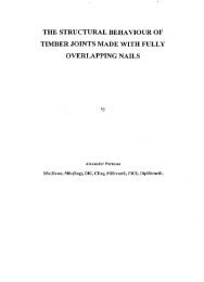
Figure 1.3 : Profile of Drum Sands in relation to height above chart datum, showing<br />
the position of the study area.<br />
All the sampling was carried out within the 250x400m study area shown in Figure 1.2,<br />
just above mean low water neap tide level (Figure 1.3). This location was chosen<br />
since preliminary sampling revealed that P. elegans patches occurred in this region<br />
and that the sedimentary conditions were relatively constant. The tide covers the<br />
whole survey area in about 15 minutes (spring tide) so tidal effects on species<br />
distributions can essentially be ignored.<br />
Very little macrobenthic data were available for Drum Sands. The sandflat is not<br />
monitored by the FRPB and the area has not previously been used for benthic studies.<br />
Stephen (1929) reported a Cerastoderma edule community on Drum Sands, but his<br />
samples were taken near Barnbougle Castle where the sediments are quite different<br />
from those found within the present study area.<br />
14
CHAPTER 2<br />
THE SMALL- To MESO-SCALE SPATIAL DISTRIBUTION OF<br />
MARINE BENTHIC INVERTEBRATES ON DRUM SANDS, WITH<br />
PARTICULAR REFERENCE TO PYGOSPIO ELEGANS<br />
INTRODUCTION<br />
Spatial heterogeneity is a fundamental characteristic of animal and plant populations<br />
(Connell, 1963; Taylor, 1984), as well as the physical environment which the<br />
organisms inhabit. The assessment of the spatial variability of some variable, e.g.,<br />
abundance of an organism, is often the starting point from which questions and<br />
hypotheses about important processes on the population or community level are<br />
generated (Andrew and Mapstone, 1987; Myers and Giller, 1988; Levin, 1992).<br />
Furthermore, Hall et al. (1993) recommended that an analysis of spatial pattern in<br />
both field experiments and survey programmes should be a priority for benthic<br />
ecologists.<br />
There are numerous techniques available for the identification of spatial pattern, such<br />
as spectral analysis (Renshaw and Ford, 1984), quadrat-variance (Greig-Smith, 1952),<br />
spatial autocorrelation analysis (Cliff and Ord, 1973; Legendre and Fortin, 1989),<br />
dispersion indices (Morisita, 1962; Elliot, 1977; Krebs, 1989) and nested hierarchical<br />
analysis of variance (Morrisey et al., 1992; Lindegarth et al., 1995). These different<br />
techniques all provide different information on spatial pattern, require different<br />
sampling strategies and are more or less suitable at different spatial scales. For<br />
example, while a hierarchical nested analysis of variance requires a nested sampling<br />
design and is most suitable for determining large-scale (100m-kms) variation<br />
(Lindegarth et al., 1995), spatial autocorrelation analysis, which requires a more<br />
regular sampling design (Thrush et al., 1989) determines the underlying spatial<br />
structure and is more suitable for smaller-scale investigations (Morrisey et al., 1992).<br />
Methods such as Greig-Smith's (1952) quadrat-variance technique, or related<br />
techniques such as the paired-quadrat variance (PQV) and two-term local quadrat<br />
15
variance (TTLQV) techniques (see Ludwig and Reynolds, 1988) assess patch sizes<br />
from a grid (or transect) of contiguous samples only.<br />
Characterisation of populations in space requires the definition of both 'intensity' and<br />
'form' (Pielou, 1969; Thrush et al., 1989; Thrush, 1991). The intensity of a spatial<br />
distribution refers to whether it is clumped, regular or not significantly different from<br />
random, while the form of a pattern describes the size of the patches or gradients<br />
(Thrush, 1991). Methods which sort distributions into clumped, regular or random,<br />
e.g., dispersion indices, rely on the distribution of density estimates about the mean<br />
rather than the actual spatial arrangement of individuals and are therefore dependent<br />
on the size of the sampling unit. Dispersion indices, although only giving information<br />
about the intensity of the pattern, have been widely used by benthic ecologists for<br />
assessing the degree of aggregation or uniformity of species distributions (e.g., Gage<br />
and Geekie, 1973; Levin, 1981; Volckaert, 1987; Meire et al., 1989; Thrush et al.,<br />
1989; Lamont et al., 1995; Lawrie, 1996). Indices such as the variance to mean ratio<br />
or index of dispersion (0, Morisita index (Id), the standardised Morisita index (/),) and<br />
Green's coefficient have been commonly applied to species data from a wide variety<br />
of sampling designs. Such indices are simple to calculate and the majority of them<br />
can be easily tested for significance using the Chi-square distribution. However, none<br />
of these indices on their own are ideal since they tend to be affected by population<br />
density and/or sample size (Elliot, 1977; Taylor, 1984; Andrew and Mapstone, 1987;<br />
Meire et al., 1989; Hurlbert, 1990). Myers (1978) suggested that several indices<br />
should be used in conjunction and when their results correspond, a stronger statement<br />
can be made about the dispersion.<br />
Dispersion indices give an indication of the intensity of pattern only, since they do not<br />
utilise the information contained in the arrangement of individuals in space they<br />
cannot give any idea as to the form of a pattern. Consequently, two distributions<br />
which may have a similar intensity of pattern may have very different spatial<br />
arrangements (Thrush, 1991; Hall et al., 1993). Furthermore, such indices give no<br />
indication of the scales at which pattern might be found other than the scale at which<br />
the data used to calculate them were gathered (Hill, 1973).<br />
16
Spatial autocorrelation analysis assesses whether the abundance of a species from one<br />
sample is significantly dependent on the abundances in neighbouring samples using<br />
Moran's 'V and/or Geary's 'c' coefficients, or the Mantel coefficient for the<br />
multivariate situation (Sokal, 1986; Sokal and Thomson, 1987; Legendre and Fortin,<br />
1989; Wartenberg, 1989). Correlograms, or graphs of these autocorrelation<br />
coefficients for various distance classes, allow inferences to be made on a variety of<br />
spatial patterns, heterogeneity in abundance, patch size and density gradients (Sokal<br />
and Oden, 1978; Sokal, 1979). Oden and Sokal (1986) and Sokal (1986) suggested<br />
that since correlograms describe the underlying spatial relationships of a pattern rather<br />
than its appearance, they may be closer guides to some of the processes that have<br />
generated these patterns than the patterns themselves. Consequently, spatial<br />
autocorrelation analysis has been widely used in many areas of ecology (Legendre and<br />
Trousellier, 1988; Leduc et al., 1992; Hinch et al., 1993; Diniz-Filho and Bini, 1994;<br />
Burgman and Williams, 1995) as well as in marine benthic studies (Jumars, 1978;<br />
Eckman, 1979; McArdle and Blackwell, 1989; Thrush et al., 1989; Lawrie, 1996;<br />
Hewitt et al., 1997) to describe the spatial pattern exhibited by macrobenthic<br />
populations and to help elucidate the processes producing them. The pattern observed<br />
depends upon the grain, lag and the extent and, therefore, there is a limit to the scales<br />
of patterns detected within any one survey.<br />
Since correlograms may only ambiguously correspond to a single type of spatial<br />
structure (Sokal and Oden, 1978) their interpretation should be complemented by<br />
maps representing the spatial variation of the variable(s) of interest (Legendre, 1993).<br />
The easiest way to obtain a contour map of a single variable is to use inverse-square<br />
distance or other interpolation methods, such as kriging. However, interpretation of<br />
interpolation plots may be subjective: the patterns produced depend to a certain extent<br />
on the interpolation method and the distance classes chosen.<br />
This study involved a detailed investigation into the spatial patterns exhibited by<br />
macrobenthic invertebrate species on an intertidal sandflat using some of the above<br />
described numerical techniques including the variance to mean ratio, Morisita index<br />
and standardised Morisita index, mapping with kriging and spatial autocorrelation<br />
17
analysis using Moran's and Geary's coefficients. An initial assessment of the spatial<br />
patterns of P. elegans will help identify which processes possibly determine this<br />
species' spatial distribution on Drum Sands and therefore the focus of successive<br />
research. The main aims of this study were:<br />
1 - to investigate the small- and meso-scale spatial distributions of macrobenthic<br />
invertebrate species and sediment variables on an intertidal sandflat;<br />
2 - to determine whether the abundance of this dominant species was associated with<br />
the spatial pattern of other species.<br />
This was accomplished firstly by an investigation into the scales of spatial variability<br />
using analysis of variance; this `transece survey was also to serve as a pilot survey. A<br />
pilot survey was considered necessary to assess the macrofaunal densities and the<br />
scales of variability present. A more detailed investigation of spatial patterns was then<br />
carried out using three grid surveys, each conducted at different spatial scales. Since<br />
patchiness may occur at many scales (Kotliar and Wiens, 1990) it is necessary to<br />
sample as many scales as possible since whether a pattern is detected or not is a<br />
function of the sampling regime (Legendre and Fortin, 1989). For example, with<br />
spatial autocorrelation analysis, patches can only be detected if the spacing of the<br />
samples is on average less than the average diameter of a patch (Sokal and<br />
Wartenberg, 1981).<br />
18
METHODS<br />
Scales of Spatial Variability - Transect Survey<br />
Survey design - The `transece survey for investigating the scales of spatial variability<br />
was carried out between the 17 and 18th of March, 1996. This survey used 16 plots<br />
arranged as shown in Figure 2.1. This design enabled the investigation of different<br />
scales of variation (patchiness) within the site using replicates within plots. The<br />
design can be described as 4 transects, 133m apart, with 4 plots along each, separated<br />
by 20m, 80m and 150m. Therefore, maximum scales of variability, in one direction<br />
only, within the area of relatively homogeneous sediments outlined in Figure 1.2 were<br />
investigated with this design.<br />
Within each plot (1x1m), 3 randomly positioned box-core samples (25x25cm, 15cm<br />
depth) were taken and the sediments sieved through a 0.5mm mesh sieve. The<br />
samples were then fixed and preserved with saline formaldehyde solution (10%),<br />
neutralised with 0.2% sodium tetraborate (Borax) with a Rose Bengal (0.01%) stain<br />
and stored. The samples were later washed with water to remove the formaldehyde<br />
and the fauna sorted in a sorting tray with the aid of a magnifying lens and stored in<br />
70% ethyl alcohol before identification. The fauna were identified to the lowest<br />
possible taxonomic level and counted. Capitella spp., which is known to be<br />
comprised of a morphologically similar but genetically distinct, sibling species were<br />
recorded as Capitella capitata (Grassle, 1984) for all of the studies carried out on<br />
Drum Sands. Pleijel and Dales (1991) suggested that Eteone flava and Eteone longa<br />
could represent two sibling species and that it is difficult to distinguish between them<br />
with preserved samples. Consequently, these individuals are called Eteone cfflava for<br />
this study.<br />
Sediment samples were taken for organic carbon analysis and particle size analysis<br />
using a corer (2.4cm internal diameter) to a depth of 3cm and frozen at -20°C for<br />
storage. These samples were taken to 3cm depth since preliminary studies found the<br />
majority of the fauna inhabited sediments above this depth. Three randomly placed<br />
sediment samples were taken within each plot and pooled. Organic carbon content<br />
determination was done by weight loss on ignition at 480°C for 4 hours. Particle size<br />
distribution analysis was performed using the 'clean beach sand' method described in<br />
19
Holme and McIntyre (1984). Percentage silt/clay (%
sediment cores. This concern for the mis-match of sampling-scales for the sediments<br />
and fauna applies to all the studies described in this thesis.<br />
Data analyses - The data for each species with a mean abundance of 2 or more<br />
individuals per core for any one transect were checked for normality using the<br />
Anderson-Darling test and for homogeneity of variance using the Bartlett test. Any<br />
data not complying with these tests were log(x+1)-transformed before statistical<br />
analysis. Any species data with a non-normal distribution or a heterogeneous variance<br />
after transformation were analysed using non-parametric statistics. Variability along<br />
each transect was assessed by either a One-way ANOVA test with a Tukey multiple<br />
comparison test or a Kruskal-Wallis test using Minitab 10.0. In the event of a<br />
significant Kruskal-Wallis test, a post hoc Tukey test was performed on the log(x+1)-<br />
transformed data to indicate which plots were significantly different from each other.<br />
21
Pattern Analysis - Grid Surveys<br />
Survey design - Statisticians have usually condemned systematic sampling in favour<br />
of random sampling (Krebs, 1989). However, McArdle and Blackwell (1989) stated<br />
that when investigating spatial patterns a systematic sampling design (e.g., grid<br />
sampling) will usually provide the smallest sampling error of the mean (Milne, 1959).<br />
The possibility of a periodic variation in the variable being studied leading to a biased<br />
estimate of the mean is negligible (Milne, 1959; Krebs, 1989). Another advantage of<br />
grid sampling is the ease with which spatial patterns can be detected and displayed<br />
(McArdle and Blackwell, 1989). Consequently, this type of sampling is<br />
recommended in pattern analysis studies (Greig-Smith, 1952; Angel and Angel, 1967;<br />
Pielou, 1969; Hill, 1973; Elliot, 1977; Jumars et al., 1977).<br />
Pattern analysis was carried out by performing 3 separate surveys, each at a different<br />
scale (lag). The sample designs for each of these grid surveys were very similar to<br />
each other (Figure 2.2), except the lags were different in each case. The lags used for<br />
the 3 surveys were lm, 8m and 40m and, from here-on will be referred to as the 1 m,<br />
8m and 40m surveys respectively. These lags were chosen so that spatial patterns<br />
could be investigated at a relatively small scale (1m survey), at an intermediate scale<br />
(8m survey) and at a relatively large scale (40m survey) within the 400x250m study<br />
area. The lm and 8m surveys were composed of plots forming an 8x8 array while<br />
those of the 40m survey formed a 9x7 array so that the design could be positioned<br />
within the study area. The positions of the lm and 8m surveys were determined by<br />
random co-ordinates while the 40m survey covered the majority of the 250mx400m<br />
survey area.<br />
At each plot faunal abundances were assessed in two ways. A single box-core sample<br />
(625cm2) was taken in an identical manner as described for the pilot survey: this<br />
method sampled the majority of the faunal species present. The results from the<br />
transect survey revealed that the lugworm Arenicola marina and the sandmason<br />
Lanice conchilega could not be sampled in this way since the majority of these<br />
individuals live deeper in the sediments than 15cm. Ragnarsson (1996) suggested that<br />
there was almost a 1:1 relationship between A. marina individuals and their casts on<br />
the Ythan Estuary, Aberdeenshire, and by direct observations (following Carey, 1982)<br />
22
that at least 90% of L. conchilega tube-heads contained live worms. Therefore, for the<br />
grid surveys the relative abundances of A. marina and L. conchilega were estimated<br />
by counting the numbers of casts and tube-heads (respectively) within a 1m 2 area<br />
around each plot. Consequently, for these two species, the grain was extended. The<br />
difference in grain used for these two species must be remembered when comparing<br />
their distributions with the other fauna since the numbers in the larger sampling unit<br />
would have been less sensitive to the presence of smaller-scale (i.e.,
57 64<br />
1=1 0 0 0 0 0 0 0<br />
O 0 0 0 0 0 Ei EI<br />
O 0 0 0 0 0 0 0<br />
O 0 0 0 0 0 0 0<br />
O 0 0 0 0 0 0 0<br />
O 0 0 0 0 0 0 0<br />
O 0 0 0 0 0 0 0<br />
1 8<br />
O 0 0 0 0 0 0 0<br />
-A<br />
-4----111. GRAIN<br />
LAG<br />
EXTENT<br />
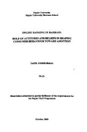
Figure 2.2 : Sample layout of the lm and 8m grid surveys showing positions of plot<br />
numbers 1, 8, 57 and 64. For the lm survey, the lag was lm and for the 8m survey,<br />
8m. The 40m survey had a similar design except a 9x7 grid was formed instead of an<br />
8x8, with a 40m lag. One box-core sample (25x25cm, 15cm depth) was taken at each<br />
plot together with 3 sediment cores (2.4cm internal diameter, 3cm depth) which were<br />
pooled. The numbers of A. marina and L. conchilega were estimated by the numbers<br />
of casts and tube-heads respectively in a 1m 2 area around each plot.<br />
Data analyses - Dispersion indices were calculated for each taxon with a mean<br />
abundance of at least 2 individuals per plot. This cut-off abundance was decided to<br />
limit the analyses to those taxa which were sufficiently abundant to allow a reasonable<br />
investigation of their spatial patterns. The dispersion indices calculated were the<br />
24
variance to mean (v:m) ratio, I; Morisita's index, Id; and the standardised Morisita's<br />
index of dispersion, Ip. These calculations were performed on the abundance data<br />
using the NEGBJNOM program (Krebs, 1989). This program gives each of these<br />
index values and indicates whether the v:m ratio is significantly different from 1:1.<br />
Departures from randomness of Id were addressed for significance (p
Maps produced by kriging and other suitable interpolation methods were essentially<br />
similar.<br />
Spatial autocorrelation analysis was carried out using the Spatial Autocorrelation<br />
Analysis Program (SAAP) version 4.3 (Wartenberg, 1989). This package produces<br />
correlograms of autocorrelation coefficient values against each distance class.<br />
Moran's `i' and Geary's 'c' autocorrelation coefficients (Cliff and Ord, 1973) were<br />
calculated in the present study since these are the most commonly used and have been<br />
recommended for use in ecological applications (Sokal, 1979; Hubert et al., 1981;<br />
Legendre and Fortin, 1989). The SAAP program gives i values in the range 1 to -1<br />
and c values in the range 0-2; while low values of i correspond to negative<br />
autocorrelation and high values correspond to positive autocorrelation, the opposite<br />
applies for values of c. Each coefficient is sensitive to slightly different behaviours of<br />
the data (Jumars et al., 1977). For example, i bears a close resemblance to a Pearson<br />
product moment correlation coefficient and is therefore most sensitive to extreme<br />
values in the data set while c, which is a distance-type function, is most sensitive to<br />
the proximity of similar or dissimilar values, regardless of their departure from the<br />
mean (Jumars eta!., 1977).<br />
Following Oden (1984) the overall significance of each spatial autocorrelogram was<br />
assessed by checking that the most significant spatial autocorrelation coefficient found<br />
in a correlogram was significant at a Bonferroni-corrected significance level a', where<br />
a'=a/k, k being the number of autocorrelation coefficients (i.e., the number of<br />
distance classes) in the correlogram (Sokal, 1986). Spatial autocorrelation analysis<br />
allowed the nature of patterns and estimates of patch sizes to be made in this study.<br />
The spatial characteristics of patches indicated by autocorrelation analysis were only<br />
accepted if the contour plots were consistent with these patterns.<br />
26
RESULTS<br />
Scales of Spatial Variability - Transect Survey<br />
From the 48 faunal samples taken for this survey, 3062 individuals were collected<br />
from a total of 48 taxa. By far the most abundant (2508 individuals) and diverse<br />
group was the polychaetes, 26 species from 13 families. The second most abundant<br />
group was the molluscs (262 individuals) with 8 species from 4 families. 257<br />
individuals were collected from the crustaceans; 12 species from 7 families.<br />
Most of the species sampled were too rare for numerical analyses, i.e., means of
200<br />
180<br />
1160<br />
140<br />
100<br />
1-3 80<br />
g 60<br />
c.)<br />
8<br />
Species Transect 20m 80m 100m 150m 230m 250m<br />
P. elegans 1 Yes<br />
C. edule 1 Yes<br />
2 Yes Yes Yes<br />
3 Yes Yes Yes<br />
4 Yes Yes<br />
C. capitata n/s<br />
N. hombergii 3 Yes<br />
E. cfflava 1 Yes<br />
B. sarsi n/s<br />
Table 2.1: Scales of variability found to be statistically significant using One-way<br />
ANOVA with a Tukey multiple comparison test at 5% level of significance for P.<br />
elegans, C. capitata and C. edule on log(x+1)-transformed data and Kruskal-Wallis on<br />
the raw abundance data for E. cfflava, M. balthica and B. sarsi with post hoc Tukey<br />
test. 'Yes' indicates statistical significance and n/s represents not significant at any<br />
scale for all transects.<br />
The results of the sediment organic content and granulometric analyses are presented<br />
in Figures 2.4(i-iv) showing the % silt/clay, % organics, Md phi and the sorting<br />
coefficient values for each plot along transects 1-4. Due to different sampling<br />
protocols and to the random positioning of sediment cores within plots rather than<br />
within faunal cores, correlation analysis between sediment properties and faunal<br />
abundances cannot be unequivocally carried out. These results, however, do suggest<br />
that there were no distinct patches or definite gradient in the environmental variables<br />
measured within the study area. Although the values did vary along and between<br />
transects it is not possible to assess whether these are significant differences without<br />
replication. The sediments of the study site have silt/clay contents of 0.50-2.89%;<br />
organic carbon contents of 0.95-2.08%; Md phi of 2.57-2.89 (fine sand) and sorting<br />
coefficients of between 0.52-0.80 (moderately sorted to moderately well-sorted).<br />
29
2.5<br />
1.5<br />
0.5<br />
0<br />
3 T<br />
(i) % Silt/clay% Organics<br />
2.5<br />
—<br />
0 50 100 150 200 250 0 50 100 150 200 250<br />
Distance along transect (m) Distance along transect (m)<br />
1.5<br />
0.5<br />
(iv) Sorting coefficient<br />
0.1 —<br />
2 I I I I I<br />
I 1 I I<br />
I<br />
0 50 100 150 200 250 0 50 100 150 200 250<br />
Distance along transect (m) Distance along transect (m)<br />
Figures 2.4(i-iv) : Sediment results from transect survey. Values of (i) % silt/clay, (ii)<br />
% organics, (iii) Md phi and (iv) Inclusive Graphic Standard Deviation (I.G.S.D.)<br />
sorting coefficient are given for each distance along transect (in metres) for all 4<br />
transects.<br />
30<br />
cd<br />
1 —<br />
0.9 —<br />
0.4 —<br />
0.3 —<br />
0.2 —<br />
•
Pattern Analysis - Grid Surveys<br />
A total of 31, 31 and 33 taxa were collected from the lm, 8m and 40m surveys<br />
respectively. A full species list, together with abundances per plot for each survey, are<br />
given in Appendices 1.1, 1.2 and 1.3 for the lm, 8m and 40m surveys respectively.<br />
Species are listed in the Appendices in the order according to Howson and Picton<br />
(1997). From these 3 surveys, 9, 10 and 11 taxa respectively were considered<br />
sufficiently abundant for pattern analysis, i.e., a mean abundance of at least 2<br />
individuals per core. Since these surveys were carried out during the summer, the<br />
abundances of the majority of the species were greater than found from the transect<br />
survey. Tables 2.2-2.4 show the dispersion indices; v:m, Id and Ip, for each of these<br />
taxa from each grid survey with the distributions they imply. There was a very good<br />
agreement between the 3 indices used. Therefore, one can be confident that the<br />
distributions inferred from these indices are correct.<br />
The results from the lm survey suggest that at this scale, 7 of the 9 species showed an<br />
aggregated distribution. These were P. elegans, A. marina, L. conchilega, E. cf flava,<br />
M. balthica, B. sarsi and G. duebeni. The distributions of N. hombergii and C. edule<br />
were not significantly different from random. Of the 10 species sufficiently abundant<br />
for analysis from the 8m survey, 8 were aggregated, i.e., P. elegans, S. martinensis, L.<br />
conchilega, C. capitata, E. cf flava, M. balthica, G. duebeni, and C. edule. N.<br />
hombergii and A. marina were found to be randomly distributed. All 11 species<br />
analysed from the 40m survey were found to have significantly aggregated<br />
distributions.<br />
Pygospio elegans had by far the greatest v:m ratio in each of the grid surveys, i.e.,<br />
31.69, 68.46 and 64.58 for the lm, 8m and 40m surveys respectively. This suggests<br />
that this species showed a high spatial variability even at relatively small scales (1m<br />
survey), forming patches within which their densities were far greater than those in<br />
surrounding non-patch areas.<br />
31
v : m pattern Id pattern Ip pattern<br />
P. elegans 31.69 ***A 1.944 *A 0.507 *A<br />
A. marina 1.58 **A 1.156 *A 0.501 *A<br />
L. conchilega 8.79 ***A 2.846 *A 0.514 *A<br />
N. hombergii 1.08 Random 0.018 Random 0.109 Random<br />
E. cf flava 2.14 ***A 1.664 *A 0.504 *A<br />
M. balthica 5.09 ***A 1.431 *A 0.503 *A<br />
C. edule 0.91 Random 0.986 Random -0.143 Random<br />
B. sarsi 5.95 ***A 4.093 *A 0.523 *A<br />
G. duebeni 4.27 ***A 2.505 *A 0.511 *A<br />
Table 2.2 : Indices of dispersion for each of the taxa in the lm grid survey. The<br />
results from the variance to mean ratio, Morisita's index (Id) and standardised<br />
Morisita's index (In) are given together with the type of dispersion/pattern they<br />
suggest (A=Aggregated) and the significance level. * Denotes significance at p
v : m pattern Id pattern Ip pattern<br />
P. elegans 68.46 ***A 2.164 *A 0.509 *A<br />
S. martinensis 7.81 ***A 2.289 *A 0.510 *A<br />
A. marina 1.26 Random 1.073 Random 0.349 Random<br />
L. conchilega 9.76 ***A 2.889 *A 0.514 *A<br />
C. capitata 53.24 ***A 8.217 *A 0.557 *A<br />
N. hombergii 1.12 Random 1.027 Random 0.152 Random<br />
E. cfflava 1.65 ***A 1.179 *A 0.501 *A<br />
M. balthica 15.22 ***A 2.605 *A 0.512 *A<br />
C. edule 25.13 ***A 1.424 *A 0.503 *A<br />
G. duebeni 11.89 ***A 9.681 *A 0.567 *A<br />
Table 2.3 : Indices of dispersion for each of the taxa in the 8m grid survey. The<br />
results from the variance to mean ratio, Morisita's index (I d) and standardised<br />
Morisita's index (Jr) are given together with the type of dispersion/pattern they<br />
suggest (A=Aggregated) and the significance level. * Denotes significance at p
" v : m pattern Id pattern Ip pattern<br />
P. elegans 64.58 ***A 2.049 *A 0.510 *A<br />
S. martinensis 5.34 ***A 3.265 *A 0.517 *A<br />
A. marina 1.74 ***A 1.159 *A 0.501 *A<br />
L. conchilega 33.55 ***A 4.336 *A 0.527 *A<br />
C. capitata 3.24 ***A 1.893 *A 0.506 *A<br />
N. hombergii 1.39 *A 1.124 *A 0.500 *A<br />
E. cfflava 2.67 ***A 1.551 *A 0.503 *A<br />
M. balthica 32.18 ***A 2.311 *A 0.510 *A<br />
C. edule 5.72 ***A 1.260 *A 0.502 *A<br />
B. sarsi 15.71 ***A 6.301 *A 0.542 *A<br />
G. duebeni 12.46 ***A 3.682 *A 0.521 *A<br />
Table 2.4 : Indices of dispersion for each of the taxa in the 40m grid survey. The<br />
results from the variance to mean ratio, Morisita's index (Id) and standardised<br />
Morisita's index (4) are given together with the type of dispersion/pattern they<br />
suggest (A=Aggregated) and the significance level. * Denotes significance at p
Table 2.5 shows the results of Spearman Rank Correlation analyses of P. elegans with<br />
other species present and the 4 sediment variables measured. Only those species with<br />
a mean abundance of at least 4 individuals per core (or per m 2 for A. marina and L.<br />
conchilega) were used for correlation analyses with P. elegans. This was to limit the<br />
number of correlations to prevent relatively low p values being non-significant after a<br />
Bonferroni correction. Therefore, correlation analysis was performed on P. elegans<br />
abundances with the abundances of M. balthica, C. edule, A. marina, and L.<br />
conchilega, together with those of C. capitata (8m survey only). The sediment<br />
variables were % organic carbon, % silt/clay content, Md 4) and sorting coefficient.<br />
lm 8m 40m<br />
rs P rs P rs P<br />
M. balthica 0.244 0.052 0.674
The results show that at the smaller scale, i.e., lm survey, P. elegans distribution was<br />
not correlated with any species nor with any sediment variable. The results from the<br />
8m survey suggest that at this scale, P. elegans was positively correlated with M.<br />
balthica and all the sediment variables, i.e., % organic carbon, % silt/clay, Md 0 and<br />
sorting coefficient, and negatively correlated with A. marina. At the larger scale, i.e.,<br />
40m survey, P. elegans was only positively correlated with M. balthica and all the<br />
sediment variables, except Md (1). The significant correlations of P. elegans<br />
abundances with those of A. marina and the sediment variables must be treated with<br />
caution because of the differences in sampling protocols (see Methods).<br />
Some of the correlations which were significant even after the Bonferroni correction,<br />
which Legendre and Legendre (1997) suggested was overly conservative and often led<br />
to rejecting too few hypotheses, appeared only weakly correlated when their scatter<br />
plots were examined. This was because the numbers of degrees of freedom (i.e., 64)<br />
were so high that even relatively low values of the coefficient, e.g., 0.401 for %<br />
organic carbon content from 40m survey, were significant. Fowler and Cohen (1990)<br />
suggested that this correlation coefficient should be used only when the number of<br />
sampling units is 30 or less. Therefore, caution is needed in the interpretation of these<br />
correlation results and thus it is important to examine the contour maps when<br />
interpreting them.<br />
lm survey - spatial patterns<br />
The contour maps presented in Figures 2.5(i-vii) display the distributions of the most<br />
abundant species from the lm survey which had significantly non-random<br />
distributions, and Figures 2.6(i-v) present the significant correlograms from spatial<br />
autocorrelation analysis. The distance classes 1-6 in Figures 2.6(i-ix) represent those<br />
samples that are 0-1m, 1-1.5m, 1.5-2m, 2-2.5m, 2.5-3m and 3-3.5m apart respectively.<br />
These were chosen instead of larger intervals so that a more accurate estimate of patch<br />
size could be achieved.<br />
Sokal (1979) described the inferences which can be made about the spatial<br />
distributions of biological populations from autocorrelation analysis and provided<br />
some useful examples. Low-order (short-distance) positive autocorrelation, where<br />
36
neighbouring samples usually assume similar values, may arise from gradients or<br />
patches exceeding the diameter of inter-sample distances. Significant positive<br />
autocorrelation (high Moran's i and low Geary's c) at distance class 1 therefore<br />
implies a patch size of between 1-1.5m2 and at distance class 2, a patch size of 1.5-<br />
2m2.<br />
Generally, there were very good agreements between the two autocorrelation<br />
coefficients used: Geary's coefficient was nearly always significant when Moran's<br />
coefficient was significant and both gave similar estimates of patch sizes in most<br />
cases. Cliff and Ord (1973) proposed that i was generally better than c, although the<br />
margin of the advantage was slight. Therefore, patch sizes are given here as indicated<br />
by Moran's coefficient.<br />
The density plots (Figures 2.5(i-vii)) suggest that all of the species with significantly<br />
non-random distributions formed areas of increased densities, or patches, of either less<br />
than 1m2 (e.g., M. balthica and E. cf flava) or between 1-2m 2 (e.g., P. elegans, A.<br />
marina, L. conchilega, G. duebeni and B. sarsi) with very low abundances outside the<br />
patches. However, mapping only gives a guide to spatial patterns, they do not confirm<br />
them. The patterns indicated in Figures 2.5(i-vii) are supported by their correlograms.<br />
For example, patch sizes smaller than inter-sample distances (or lag, in this case 1m)<br />
are not revealed by spatial autocorrelation analysis and therefore M. balthica and E. cf<br />
flava had non-significant correlograms. For these species, smaller inter-sample<br />
distances would have been needed to determine their underlying spatial structure. The<br />
significant correlograms with positive autocorrelation at distance class 1 indicate that<br />
P. elegans, A. marina, L. conchilega and G. duebeni formed patches of 1-1.5m2 while<br />
the positive autocorrelation at distance class 2 suggests that B. sarsi formed patches of<br />
1.5-2m2. For P. elegans, 2 patches were sampled wholly within the 8x8m grid, with 3<br />
others on the edge. These corresponded to the positions of areas of smooth, raised<br />
sediment (pers. obs.) and therefore confirm that these areas did indeed contain<br />
significantly increased numbers of P. elegans. Furthermore, Figure 2.5(i) shows that<br />
although the patch sizes were approximately equal, the inter-patch distances varied<br />
suggesting that the P. elegans patches were randomly distributed at this scale.<br />
37
Nephtys hombergii's spatial distribution produced a significant correlogram (Figure<br />
2.6v) even though its distribution was not significantly different from random (Table<br />
2.2). The correlogram implies that N. hombergii formed patches between 1-1.5m2<br />
which were 1.5-2m apart, this is supported by its density plot, Figure 2.5(viii).<br />
Similarly, Thrush et al. (1989) found that some species which were randomly<br />
distributed according to their indices of dispersion did in fact have significant spatial<br />
structures.<br />
Figures 2.5(ix-xii) display the spatial heterogeneity of % organic carbon, % silt/clay,<br />
Md (1) and sorting coefficient. These sediment variables also appeared clumped:<br />
patches of increased organic carbon and silt/clay contents, together with areas of<br />
higher Md Os and sorting coefficients, were present. These patches appeared larger<br />
than those formed by most of the faunal species analysed. The significant<br />
correlograms presented in Figures 2.6(vi-ix) suggest spatial structures with patch sizes<br />
1.5-2m2 for % organic content, % silt/clay and sorting coefficient and >3.5m 2 for Md<br />
(1). Within these patches, sediments contained higher levels of these variables<br />
compared to surrounding sediments. According to their contour plots, these 4<br />
sediment variables appeared to have been positively correlated with each other in their<br />
spatial distributions. A comparison of the spatial heterogeneity of these sediment<br />
variables with those of the fauna must be made with caution due to the mis-match of<br />
scales (see Methods). Although % organic content, % silt/clay and sorting coefficient<br />
formed patches similar in size (1.5-2m 2) to many of the species the contour plots<br />
suggest that they were not spatially correlated. This was formally tested for P. elegans<br />
(Table 2.5) but the density plots suggest that this appears to have been the case for all<br />
the other species.<br />
Figures 2.5(i-xi) support the results of the correlation analyses. For example, high<br />
density areas, or patches, of P. elegans did not occur in the same areas as those formed<br />
by other species, nor did they appear in the same areas as high levels of the 4 sediment<br />
variables.<br />
38
Cm<br />
7m<br />
.11111.11011111011W<br />
4m 5m<br />
N P. elegans<br />
4i71<br />
(iii) L. conchilega<br />
(v) M. balihica<br />
701<br />
200<br />
190<br />
180<br />
170<br />
160<br />
150<br />
140<br />
130<br />
120<br />
110<br />
, 100<br />
- so<br />
80<br />
70<br />
- so<br />
so<br />
40<br />
30<br />
20<br />
10<br />
26<br />
24<br />
22<br />
20<br />
18<br />
16<br />
14<br />
12<br />
10<br />
8<br />
6<br />
4<br />
2<br />
-2<br />
38<br />
1, 32 30<br />
36<br />
34<br />
28<br />
26<br />
24<br />
22<br />
-;2o<br />
18<br />
16<br />
14<br />
12<br />
10<br />
Figures 2.5(i-vi) : Contour map of species abundances and sediment variables<br />
from lm survey with non-random distribution using kriging.<br />
39<br />
(n) A. marina<br />
4m 5m em<br />
(iv) E. cfflava<br />
(vi) B. sarsi<br />
7m<br />
• a•<br />
10.0<br />
9.5<br />
9.0<br />
8.5<br />
8.0<br />
7.5<br />
7.0<br />
6.5<br />
6.0<br />
5.5<br />
5.0<br />
4.5<br />
4.0<br />
3.5<br />
3.0<br />
2.5<br />
2.0<br />
1.5<br />
1.0<br />
0.5<br />
0.0<br />
-0.5<br />
17<br />
16<br />
15<br />
14<br />
13<br />
12<br />
11<br />
, 10<br />
71, 8<br />
7<br />
6<br />
5<br />
1<br />
0
(vii) G. duebeni<br />
(ix) % Organic content<br />
7n1<br />
15<br />
-14<br />
13<br />
-H 12<br />
11<br />
-19<br />
10<br />
5<br />
no<br />
280<br />
270<br />
260<br />
250<br />
240<br />
230<br />
220<br />
210<br />
2.00<br />
1.90<br />
t80<br />
1.70<br />
1.60<br />
1.50<br />
1.40<br />
1.30<br />
3.10<br />
3.08<br />
3.06<br />
3.04<br />
3.02<br />
3.00<br />
2.98<br />
2.96<br />
294<br />
2.92<br />
2.90<br />
2.88<br />
286<br />
2.84<br />
2.82<br />
2.80<br />
2.78<br />
Figures 2.5(vii-xii) : Continued<br />
40<br />
1m<br />
srn<br />
(vin) N. hombergii<br />
1m,<br />
1m 2m 4 501 6m 7m<br />
(x) % Silt/clay content<br />
4;r1 5n1 em<br />
(xii) Sorting coefficient<br />
•<br />
•<br />
11.0<br />
10.5<br />
10.0<br />
9.5<br />
9.0<br />
8.5<br />
8.0<br />
7.5<br />
7.0<br />
6.5<br />
60<br />
5.5<br />
5.0<br />
4.5<br />
4.0<br />
3.5<br />
3.0<br />
2.5<br />
2.0<br />
1.5<br />
1.0<br />
0.5<br />
6.00<br />
5.50<br />
5.00<br />
4.50<br />
4.00<br />
3.50<br />
3.00<br />
2.50<br />
2.00<br />
1.50<br />
1.03<br />
0.50<br />
0.00<br />
0.69<br />
0.69<br />
0.69<br />
0.68<br />
0.68<br />
0.67<br />
0.67<br />
0.66<br />
ass<br />
0.65<br />
0.64<br />
0.64<br />
0.63<br />
0.63<br />
0.63<br />
0.62<br />
0.62<br />
0.61<br />
0.61
1.3 (i) P. elegans<br />
(ii) A. marina<br />
ti.)<br />
.P.<br />
>* 0.8<br />
t<br />
T.;<br />
e<br />
8<br />
U<br />
0.3<br />
-0.2<br />
1.3<br />
0.8<br />
EE) 0.3<br />
8<br />
e4 0.3<br />
8<br />
U ..... .....<br />
2 3 4<br />
Distance class<br />
(iii) L. conchilega<br />
-0.2 2 3 4<br />
Distance class<br />
1.3 (v) N. hombergii<br />
-0.2 2 3 4<br />
Distance class<br />
1.3 (vii) % Silt/clay<br />
o . s<br />
-0.2 2 3 4<br />
Distance class<br />
1.3<br />
V. 0.8<br />
68<br />
0.3<br />
p
8m survey - spatial patterns<br />
Figures 2.7(i-viii) present the interpolated density maps of the non-randomly<br />
distributed species from the 8m survey while Figures 2.8(i-v) display the significant<br />
correlograms. The distance classes 1-6 for these correlograms represent inter-sample<br />
distances of 0-8m, 8-12m, 12-16m, 16-20m, 20-24m and 24-28m, respectively. The<br />
density maps suggest that 2 species appeared to form patches less than 8m 2 (E. cf<br />
flava and G. duebeni; both of which produced non-significant correlograms) while the<br />
other species either formed patches between 8-24m 2 (C. capitata, S. martinensis and<br />
L. conchilega) or patches of various sizes (P. elegans). The correlograms do not<br />
appear to support the density plots for all species. For example, while the density plot<br />
for L. conchilega (Figure 2.7(iii)) suggests a patch of approximately 20m 2 was<br />
present, the correlogram (Figure 2.8(ii)) implies a patch size of only 8-12m2.<br />
Areas of increased densities of some species, C. edule and M. balthica for example,<br />
were located at the edges of the 56x56m survey area and therefore it is not possible to<br />
give an indication of patch sizes from the density plots and one must be cautious when<br />
drawing conclusions from their correlograms.<br />
Figures 2.7(i-xii) support the results of the correlation analyses (Table 2.5). The non-<br />
significant correlations between P. elegans and most of the other species are clearly<br />
defended by the maps since high density patches of most species do not seem to have<br />
been spatially correlated within the survey area. Furthermore, the significant positive<br />
correlation between P. elegans and M. balthica is vindicated by their contour plots,<br />
although the locations of moderate M. balthica densities as well as high densities have<br />
to be observed to see this.<br />
Figures 2.7(ix-xii) suggest that the 4 measured sediment variables were spatially<br />
correlated with each other to a certain extent. Increased levels of organic carbon and<br />
silt/clay, together with Md 0 and sorting coefficient were mainly found at the top of<br />
the 56x56m grid, although high levels of organic carbon content and Md (I) were also<br />
found in other small areas. The significant correlograms produced for the distribution<br />
of these variables (except % organic content) in Figures 2.8(vi-viii) indicate patch<br />
sizes of approximately 20-24m 2. However, since these were located at the edges of<br />
42
the survey area, one must be cautious. The significant positive correlations between<br />
P. elegans abundance and the levels % silt/clay, % organics and sorting coefficient are<br />
supported by the contour plots.<br />
40m survey - spatial patterns<br />
Figures 2.9(i-xi) present the contour maps of the non-randomly distributed species<br />
from the 40m survey and Figures 2.10(i-ix) display the significant correlograms. The<br />
distance classes 1-6 for these correlograms represent inter-sample distances 0-40m,<br />
40-60m, 60-80m, 80-100m, 100-120m and 120-140m respectively. These Figures<br />
suggest that P. elegans, E. cfflava, M. balthica and C. edule formed patches between<br />
40-60m2. Some species, S. martinensis, A. marina, L. conchilega and B. sarsi for<br />
example, formed patches which were located at the edge of the survey area and so it is<br />
difficult to estimate their patch sizes. Although not formally tested, none of the<br />
species appeared to form patches which were spatially correlated with any other<br />
species. The significant positive correlation between P. elegans and M. balthica<br />
(Table 2.5) is not strongly supported by the contour plots, although their patch sizes<br />
were similar they were not spatially correlated.<br />
Figure 2.9(xii-xv) show that the sediment variables appear to have had increased<br />
levels approximately across the middle region of the survey area. The correlograms<br />
indicated that these patches were approximately 80-100m2. The significant positive<br />
correlations between P. elegans and % organic carbon, % silt/clay and sorting<br />
coefficient (Table 2.5) were better supported by the maps for the 40m survey than they<br />
were for the 8m survey with high levels of these variables occurring at approximately<br />
the same areas as the P. elegans patches. The contour plots support the significant<br />
positive correlations between P. elegans and % silt/clay, % organics and sorting<br />
coefficient and suggest that no other species was positively correlated with them.<br />
43
(1) P. elegans<br />
(iii) L. conchilega<br />
(v) E. el:flaw<br />
240<br />
220<br />
200<br />
180<br />
160<br />
140<br />
120<br />
100<br />
80<br />
so<br />
40<br />
20<br />
0<br />
11<br />
10<br />
9<br />
8<br />
7<br />
5<br />
4<br />
3<br />
2<br />
1<br />
0<br />
-1<br />
24<br />
22<br />
20<br />
18<br />
16<br />
14<br />
10<br />
8<br />
4<br />
2<br />
0<br />
°mOm 5 'm 10m 15m 20m 2grn 30m 3n1 40m 45rn 50m 51,1<br />
(ii) S. martinensis<br />
'mDm 5m 10m 10m 20m 25m 30m 30m 40m 45m 5001 55m<br />
(i1) C. capitata<br />
vim 15m<br />
20m 25m 30rn 34 45m<br />
(w) M balthica<br />
Figures 2.7 (i-vi) : Contour maps of species abundances and sediment variables from<br />
8m survey with non-random distributions using kriging.<br />
44<br />
50m<br />
45rn<br />
4Orn-<br />
35m<br />
30m,<br />
25m-<br />
20m-<br />
15m-<br />
10m-<br />
5m-<br />
36<br />
34<br />
- 32<br />
30<br />
28<br />
26<br />
24<br />
22<br />
20<br />
16<br />
14<br />
12<br />
10<br />
8<br />
6<br />
4<br />
2<br />
0<br />
105<br />
100<br />
95<br />
90<br />
85<br />
80<br />
75<br />
-170<br />
65<br />
-- 60<br />
55<br />
50<br />
45<br />
40<br />
35<br />
30<br />
25<br />
20<br />
15<br />
10<br />
5<br />
0<br />
o 70<br />
65<br />
55<br />
50<br />
45<br />
ao<br />
35<br />
30<br />
25<br />
zo<br />
15<br />
10<br />
5<br />
0<br />
-5
50m<br />
45m<br />
4Orn<br />
35rn<br />
30m<br />
25m<br />
20m<br />
15m-<br />
10m<br />
5m<br />
(vii) C. edule<br />
(ix) % Organic content<br />
Om Om 5m 10m 1 20m 25rn 3 3 40m 45m 50m 55m<br />
(xi) Md phi<br />
190<br />
180<br />
170<br />
160<br />
150<br />
140<br />
130<br />
120<br />
100<br />
90<br />
80<br />
70<br />
60<br />
50<br />
40<br />
30<br />
20<br />
10<br />
1.10<br />
1.05<br />
1.00<br />
0.95<br />
0.90<br />
0.85<br />
0.80<br />
0.75<br />
0.70<br />
0.65<br />
0.60<br />
0.55<br />
0.50<br />
0.45<br />
0.40<br />
0.35<br />
0.30<br />
3.00<br />
2.98<br />
2.96<br />
2.94<br />
2.92<br />
2.90<br />
2.88<br />
12.86<br />
2.84<br />
2.82<br />
2.80<br />
2.78<br />
2.76<br />
2.74<br />
2.72<br />
2.70<br />
2.68<br />
2.66<br />
2.64<br />
50m<br />
45m<br />
40.n<br />
rn<br />
15m<br />
10m<br />
Figures 2.7 (vii-xii) : Continued<br />
45<br />
(viii) G. duebeni<br />
(x) % Silt/clay content<br />
Om 5m 10m 15m 20m 25m 30m 35rn 40m 45m 50m 55m<br />
(xii) Sorting coefficient<br />
011<br />
20<br />
19<br />
18<br />
17<br />
16<br />
15<br />
14<br />
13<br />
12<br />
11<br />
10<br />
8<br />
7<br />
6<br />
5<br />
4 3<br />
2 1<br />
0 -1<br />
2.0<br />
1.8<br />
1.6<br />
1.4<br />
1.2<br />
1.0<br />
0.8<br />
0.6<br />
0.4<br />
0.74<br />
0.73<br />
0.72<br />
0.71<br />
10.70<br />
0.69<br />
0.68<br />
0.67<br />
0.66<br />
0.65<br />
0.64<br />
0.63<br />
0.62<br />
0.61<br />
0.60<br />
0.59<br />
0.58
a)<br />
Ts<br />
1.4<br />
0.6<br />
u 0.2<br />
-0.2<br />
1.4<br />
'E5 0.6<br />
(1) S. martinensis<br />
p
103m 1030 200m 2050<br />
(i) P. elegans<br />
500 Warn 1500 203m 2500 300m<br />
(v) C. capitata<br />
Om 10Orn 1000 2500<br />
210<br />
200<br />
190<br />
2000 -<br />
180<br />
170<br />
160<br />
150<br />
140 1<br />
13u<br />
120<br />
. 110<br />
100<br />
90 100n<br />
80<br />
70<br />
50<br />
50<br />
40<br />
50m<br />
30<br />
20<br />
10 Zej<br />
0m NM IMMINnlnMOOMPR6-.0:06EIMInMOilfla<br />
Om 500 1000 1500 2000 2500 3000<br />
(ii) S. martinensis<br />
1<br />
14<br />
13<br />
12<br />
11<br />
10<br />
9<br />
7<br />
6<br />
5<br />
4<br />
2<br />
12<br />
11<br />
10<br />
5<br />
4<br />
3<br />
2<br />
0<br />
-1<br />
203m<br />
1500<br />
1030<br />
1000 1500 200m 500<br />
(iv) L. conchilega<br />
(vi) N. hombergii<br />
('vii) E. cfflava (viii) M balihica<br />
Figures 2.9 (i-viii) : Contour maps of species abundances and sediment variables from<br />
40m survey with non-random distributions using kriging.<br />
47<br />
is<br />
17<br />
16<br />
15<br />
14<br />
13<br />
12<br />
11<br />
10<br />
7<br />
6<br />
5<br />
4<br />
3<br />
2<br />
1<br />
0<br />
-1<br />
90<br />
85<br />
ao<br />
75<br />
70<br />
65<br />
60<br />
55<br />
50<br />
. 45<br />
- 40<br />
35<br />
30<br />
25<br />
20<br />
15<br />
10<br />
5<br />
0<br />
-5<br />
100<br />
05<br />
90<br />
85<br />
80<br />
75<br />
70<br />
65<br />
60<br />
5: 5<br />
45<br />
40<br />
35<br />
30<br />
25<br />
20<br />
15<br />
10<br />
5<br />
i -5
200m<br />
150m<br />
100m<br />
50m<br />
(ix) C. edule<br />
56,”l 200rn 250m<br />
(xi) G. duebeni<br />
50m 100m 150m 200m 250m 300m<br />
(xiii) % Silt/clay content<br />
50<br />
45<br />
40<br />
35<br />
ao<br />
25<br />
20<br />
15<br />
10<br />
40<br />
35<br />
111 30<br />
25<br />
20<br />
15<br />
10<br />
2.5<br />
2.0<br />
1.5<br />
1.0<br />
0.5<br />
0.0<br />
(xv) Sorting coefficient<br />
Figures 2.9 (ix-xv) : Continued.<br />
48<br />
.<br />
38<br />
36<br />
34<br />
32<br />
30<br />
28<br />
26<br />
24<br />
22<br />
20<br />
18<br />
16<br />
14<br />
12<br />
10<br />
a<br />
6<br />
4<br />
2<br />
0<br />
55m 20511 2500 300m<br />
i -2<br />
(x) B. sarsi<br />
70061 50m 200m 250m<br />
(xii) % Organic content<br />
668<br />
ass<br />
064<br />
0.62<br />
bri 0.60<br />
asa<br />
056<br />
0 54<br />
0.52<br />
0.50<br />
0.48<br />
0.46<br />
644<br />
(xiv) Md phi<br />
•<br />
29<br />
2.0<br />
2.7<br />
2.6<br />
2.5<br />
2.4<br />
2.3<br />
2.2<br />
2.1<br />
2.0<br />
1.9<br />
10<br />
1.7<br />
1.6<br />
1.6<br />
1.4<br />
1.3<br />
1.2<br />
3.10<br />
3.05<br />
300<br />
2.95<br />
200<br />
265<br />
2.80<br />
276<br />
2.70<br />
2.65<br />
2.60<br />
2.55<br />
i 2.50
.t 0.6<br />
0<br />
74'<br />
0.2<br />
-0.2 2 3 4 5<br />
Distance class<br />
0.6<br />
r`l 0.2<br />
-0.2<br />
1.4 (i) P. elegans<br />
p
73<br />
‘a•<br />
el<br />
1.4 (ix) G. duebeni 1.4<br />
0.6<br />
0.2<br />
-0.2 2 3 4<br />
Distance class<br />
1.4 (Xi) % Silt/clay<br />
0.6<br />
0.2<br />
— • .......<br />
p
1.4 (ix) G. dttebeni 1.4<br />
0.6<br />
0.2<br />
-0.2<br />
2 3 4<br />
Distance class<br />
1.4 (Xi) % Silt/clay<br />
0.6<br />
0.2<br />
-0.2<br />
"" -------<br />
•<br />
2 3 4 5<br />
Distance class<br />
d<br />
0.6<br />
0.2<br />
Figures 2.10(ix-xiii) : Continued.<br />
p<br />
-0.2<br />
1.4<br />
• 0.6<br />
Fe,<br />
u° 0.2<br />
-0.2<br />
1.4 (xiii) Sorting coefficient<br />
-0.2 2 3 4<br />
Distance class<br />
50<br />
(x) % Organic content<br />
- - .D-------<br />
2 3 4<br />
Distance class<br />
(xii) Md phi<br />
2 3 4<br />
Distance class<br />
p
DISCUSSION<br />
The main aims of this study were:<br />
1) to investigate the spatial heterogeneity of the macrobenthic species and sediment<br />
variables at different spatial scales on an intertidal sandflat;<br />
2) to determine whether the heterogeneity created by a dominant biogenic species<br />
affects the spatial patterns of other species.<br />
The spatial patterns of macrobenthic species and sediments on Drum Sands,<br />
Firth of Forth.<br />
This study used a variety of techniques to assess the distributions of the macrobenthic<br />
invertebrate species within the study area of Drum Sands. Firstly, a pilot survey was<br />
carried out from which spatial heterogeneity was investigated using analysis of<br />
variance. Although some species, e.g., P. elegans, C. edule and E. cf flava, had<br />
significantly different mean abundances between plots at one or more scales, this<br />
technique did not give a good insight into spatial patterns for several reasons. Firstly,<br />
the survey was carried out during March when the invertebrate abundances were<br />
generally low and secondly, although mean abundances of many taxa varied greatly at<br />
different scales, most were non-significant because of large within-plot replicate<br />
variability. This survey design is appropriate for pilot surveys giving an indication of<br />
mean abundances and variability on an intertidal sandflat but gives little information<br />
about their spatial patterns.<br />
A much more detailed assessment of spatial patterns was given by the results of the<br />
grid surveys using dispersion indices, mapping and spatial autocorrelation analysis.<br />
Spatial patterns which were exhibited over scales of about 1-120m were defined in<br />
these surveys. Patterns which occurred over the less than tens of centimetre scale<br />
were lost in the small-scale heterogeneity and this was partly defined by the<br />
constraints of the sampling design. At this scale, the spatial patterns of P. elegans<br />
within high-density patches are discussed in Chapter 7.<br />
Dispersion indices provided an assessment of the intensity of pattern but they gave no<br />
information about the form of any pattern of macrobenthic invertebrates on Drum<br />
Sands. Of the species sufficiently abundant for spatial analyses from the 1, 8 and 40m<br />
51
surveys; 7 out of 9; 8 out of 10 and 11 out of 11 species exhibited significantly non-<br />
random distributions respectively with very good agreements between the 3 dispersion<br />
indices (i.e., I, Id and /p) used. All of these were aggregated distributions, i.e., their<br />
variances were greater than their means. These dispersion indices gave a simple but<br />
useful indication as to the degree of spatial heterogeneity exhibited by many of the<br />
species within each survey. This is in agreement with many other studies of the<br />
marine benthos (e.g., Gage and Geekie, 1973; Volkaert, 1987; Meire et al., 1989;<br />
Thrush et al., 1989; Lamont et al., 1995; Lawrie, 1996). These studies have revealed<br />
that the majority of macrobenthic populations in both intertidal and sublittoral areas<br />
are aggregated and that apparent randomness or uniformity at the scales defined in the<br />
present study are rare.<br />
The lack of significance from a random distribution did not preclude a significant<br />
spatial pattern in all cases. For example, according to its dispersion indices, the<br />
distribution of N. hombergii (mean abundance of 5 individuals per core) in the lm<br />
survey was random, yet spatial autocorrelation analysis indicated that it exhibited a<br />
significant spatial structure. Gage and Geekie (1973) proposed that spatial analysis<br />
based on variance estimates is influenced by the number of individuals and<br />
consequently low density populations are less likely to show significant differences<br />
from random. This may explain why P. elegans which was by far the most abundant<br />
species had relatively high variance to mean ratios. Consequently, dispersion indices<br />
do not give reliable indications of spatial intensity for rarer species. Therefore,<br />
previous studies relying solely upon dispersion indices may have under-estimated the<br />
presence of spatial heterogeneity for low-density species.<br />
Mapping, together with spatial autocorrelation analysis, provided detailed and less<br />
equivocal assessments of the form of spatial patterns. These techniques suggested that<br />
the majority of the species within the study area indicated in Figure 1.2 formed<br />
patches of increased density at one or more scales. In the 1 m survey, 4 of the 7<br />
species with significantly non-random distributions displayed significant spatial<br />
patterns in addition to N. hombergii. These species, P. elegans, A. marina, L.<br />
conchilega, B. sarsi and N. hombergii, formed patches between 1-2m2. The other<br />
species with non-random distributions, i.e., M. balthica, G. duebeni and E. cf flava,<br />
52
formed patches less than 1m2 and thus had non-significant correlograms at this scale.<br />
At a larger scale, the 8m survey also revealed patches of different sizes, e.g., less than<br />
8m2 (P. elegans, E. cf flava and G. duebeni) and 8-24m2 (C. capitata, S. martinensis<br />
and L. conchilega). The two bivalve species M. balthica and C. edule had significant<br />
spatial structures at this scale but the sizes of their patches could not be estimated<br />
because of their location at the edge of the survey area. At the largest scale<br />
investigated, 8 of the 11 species with aggregated distributions exhibited significant<br />
spatial patterns. Many of these formed patches between 40-60m2, P. elegans, E. cf<br />
flava, C. edule and M. balthica, for example.<br />
The sediments were also spatially structured within the study area. Again, mapping,<br />
together with spatial autocorrelation analysis revealed that at the smallest scale,<br />
patches of 1.5-2m2 of increased % organic carbon content, % silt/clay and sorting<br />
coefficient were present while patches >3.5m 2 of increased median particle size (Md<br />
4)) were present. These variables formed larger patches in the 8m survey but their<br />
sizes could not be ascertained with any confidence because they were located at the<br />
edge of the survey area. The 40m survey indicated that these sediment variables<br />
formed patches approximately 80-100m 2 across the centre of the survey area.<br />
High-density patches formed by tube-dwelling polychaetes on intertidal sandflats have<br />
been well documented (e.g., Sanders et al., 1962; Daro and Polk, 1973; Dupont, 1975;<br />
Featherstone and Risk, 1977; Noji and Noji, 1991; Morgan, 1997). Patches of spionid<br />
polychaetes vary greatly in size from 0.04-9m2 (Marenzelleria viridis; Zettler and<br />
Bick, 1996) to 150,000m2 (Clymenella torquata; Sanders et al., 1962). However,<br />
comparisons of the spatial patterns identified in this study with those of tube-builders<br />
found at other intertidal sandflats are difficult since most studies have been carried out<br />
in either very different habitats and/or focused on defining smaller-scale patterns. The<br />
few studies explicitly investigating spatial distributions at this scale have found that<br />
soft-bottom macroinvertebrates generally exhibit significant spatial structuring on<br />
intertidal sandflats, forming patches of various sizes. For example, Thrush et al.<br />
(1989) investigated the spatial arrangements of polychaetes and bivalves in the<br />
intertidal sandflats of Manukau Harbour, New Zealand. Of the 36 populations<br />
studied, 30 were found to have significant spatial patterns, as assessed by variance to<br />
53
mean ratio and spatial autocorrelation analysis, forming patches of increased densities<br />
between 5 and 30m radius. McArdle and Blackwell (1989) found the bivalve Chione<br />
stutchburyi formed patches of increased density of 5-15m in a sandy lagoon in Ohiwa<br />
Harbour, New Zealand. Morrisey et al. (1992), using a nested sampling design,<br />
showed that the abundances of the infauna in the soft sediments of Botany Bay,<br />
Australia, were patchy at scales from 1 metre to several kilometres. None of the<br />
species in the study by Thrush et al. (1989) exhibited identical spatial patterns at all of<br />
the 6 sandflats which suggests that patterns and patch sizes are partly affected by their<br />
environment and that different studies are likely to give different spatial patterns for<br />
the same species. In addition, Hewitt et al. (1997) showed that spatial patterns varied<br />
temporally within the same site.<br />
Heterogeneity results from a complex interaction of biotic and abiotic processes<br />
(Livingston, 1987; Caswell and Cohen, 1991). At the scale investigated in this study,<br />
metres to tens of metres, spatial heterogeneity of macrofauna may result from many<br />
processes including disturbance, larval settlement, competition and sediment<br />
heterogeneity. In most studies, the causes of the patterns are only hypothesized or<br />
inferred from the data available. For example, Thrush et al. (1989) suggested that<br />
feeding pits generated by rays may have been responsible for the generation of small-<br />
scale heterogeneity within larger homogeneous density patches at two of their sites,<br />
while McArdle and Blackwell (1989) proposed that the pattern of C. stutchburyi at<br />
their site may have resulted from an environmental gradient. Morgan (1997)<br />
suggested that a large, gregarious settlement of larvae must have been one of the<br />
prerequisites for the formation of very dense patches of P. elegans in the intertidal<br />
sandflats of the Baie de Somme, France.<br />
Determining the process(es) responsible for an observed pattern at this scale (metres<br />
to hundreds of metres) is very difficult (McArdle et al., 1997). Although controlled,<br />
manipulative experiments are possible at smaller scales (centimetres to a metre) their<br />
conclusions cannot be scaled-up to larger scales since different processes are likely to<br />
be responsible for giving rise to patterns. For example, Hewitt et al. (1996) showed<br />
that it was possible to predict the spatial patterns (
stutchbutyi, at Wirroa island, New Zealand, based on their size, feeding mode and<br />
mobility. However, studies carried out at the same location by Legendre et al. (1997)<br />
revealed that the larger-scale patterns (10m to several 100m) of these two species were<br />
largely created by physical variables and that biotic effects were undetectable. They<br />
proposed that the reason for the disparity between the results from their study and the<br />
one by Hewitt et al. (1996) was due to scale differences.<br />
The study described here was not explicitly aimed at determining the processes<br />
responsible for any spatial patterns observed. The results from other studies, for<br />
example Hewitt et al. (1996) and Legendre et al. (1997), suggest that patchiness at the<br />
smaller scale investigated in this study (1-2m2) may have been generated by biological<br />
processes while those at larger scales (tens of metres to a hundred metres) may have<br />
resulted from physical processes. Patches between 1-2m 2 exhibited by species in the<br />
present study on Drum Sands did not appear to be spatially correlated with each other<br />
which suggests that they may have been generated either by negative interspecific or<br />
positive intraspecific interactions. Hewitt et al. (1996) showed that it was possible to<br />
infer processes from small-scale (
lack of apparent correlation must be treated with caution due to different sampling<br />
regimes for the sediments and fauna. There were significant positive correlations of<br />
P. elegans density with high levels of % organic content, % silt/clay, Md 4) and sorting<br />
coefficient in the 8m and 40m surveys. Tube-building polychaetes have been shown<br />
to affect these sediment properties (Noji, 1994; Morgan, 1997) and, therefore, the<br />
sediments may not have been responsible for the generation of P. elegans patchiness<br />
but vice versa. This will be discussed further for P. elegans on Drum Sands in<br />
Chapter 8.<br />
Drum Sands is a relatively high energy sandflat with frequent sediment movement<br />
(pers. obs.) and macroalgal mats are capable of forming during the summer (summer<br />
of 1996 for example). Therefore, the mosaic of species patches observed in this study<br />
may have been generated by disturbances. The role of disturbance in structuring<br />
macrobenthic populations on Drum Sands will be addressed in Chapters 4, 5 and 6.<br />
This study revealed spatial patterns of many common intertidal macrobenthic species<br />
found in European sandflats at various scales using regular grid-sampling techniques.<br />
This sampling design is simple to carry out, is capable of covering a range of scales<br />
and spatial patterns can be easily detected and displayed. This study revealed the<br />
presence of patches of 1-2m2 in many species.<br />
The effect of a dominant biogenic species on the spatial patterns of other<br />
invertebrate species on an intertidal sandflat.<br />
One of the most conspicuous biological features on an intertidal sandflat are the<br />
mounds or plateaus formed by high densities of tube-building polychaetes. On Drum<br />
Sands, P. elegans forms areas of smooth, raised sediment, approximately 1-1.5m2,<br />
within an otherwise wave-rippled sandflat. These areas are characterised by increased<br />
densities of P. elegans. Many studies have reported different sediment characteristics<br />
within dense arrays of tube-building polychaetes (Dupont, 1975; Featherstone and<br />
Risk, 1977; Noji, 1994; Morgan, 1997; Chapter 8) and these have resulted in different<br />
faunal assemblages (Sanders et al., 1962; Fager, 1964; Ragnarsson, 1996; Chapter 8).<br />
None of these studies, however, have assessed to what extent the spatial pattern<br />
56
exhibited by the tube-building polychaete has an effect upon the spatial pattern of<br />
other species.<br />
Species with similar structure functions (correlograms) do not necessarily occupy the<br />
same spatial locations (Hewitt et al., 1996). For example, while the correlograms of<br />
P. elegans, L. conchilega, B. sarsi and N. hombergii suggested that these species<br />
formed patches of increased densities approximately 1-1.5m2, their density plots<br />
revealed that their patches were not spatially correlated. For P. elegans, this was<br />
examined more formally using correlation analyses which supported the observations<br />
that P. elegans abundances were not correlated with the abundances of L. conchilega<br />
or M. balthica (B. sarsi and N. hombergii were not considered sufficiently abundant<br />
for correlation analyses). This suggests that the spatial patterns of P. elegans on Drum<br />
Sands did not have a large positive effect on those of the other common species.<br />
Pygospio elegans was only positively correlated with one species in this study, M.<br />
balthica (8m and 40m surveys). However, positive association does not necessarily<br />
imply a positive interaction, since negative interactions (e.g., predation) can take place<br />
between species coincident in space, or coincidence may occur due to some common<br />
ecological preference between two species. Controlled manipulative experiments,<br />
together with spatial autocorrelation analysis, are needed to test explicitly for the<br />
presence of an interaction between these two species.<br />
Tube-building polychaetes are capable of affecting species distributions via many<br />
direct and/or indirect interactions, e.g., hydrodynamic effects (Eckman et al., 1981;<br />
Eckman, 1983), provision of refuges (Woodin, 1978, 1981; Lukenbach, 1986) and<br />
increased food availability (Eckman, 1983; Noji, 1994) which suggest that the positive<br />
association between P. elegans and M. balthica in this study may have been non-<br />
coincidental. A change in spatial pattern of M. balthica or reduced survival, growth or<br />
recruitment may, therefore, be expected in the absence of P. elegans. The processes<br />
by which P. elegans affect other fauna are discussed further in Chapter 8 in which the<br />
faunal communities and sediment variables of P. elegans patches are compared with<br />
non-patch sediments using not a non-parametric correlation approach as in this study<br />
but a more suitable, parametric method of statistical analysis, i.e., t-tests.<br />
57
The study described here has provided important information about the spatial<br />
patterns exhibited by the abundant invertebrate species on Drum Sands. The results<br />
have provided invaluable information from which hypotheses can be tested about the<br />
generation of spatial patterns on intertidal sandflats, in particular, the small-scale<br />
patches formed by P. elegans and the role they play in structuring the community.<br />
58
CHAPTER 3<br />
THE POPULATION STRUCTURE AND REPRODUCTIVE<br />
BIOLOGY OF PYGOSPIO ELEGANS ON DRUM SANDS<br />
INTRODUCTION<br />
Natural and anthropogenic disturbances have been shown to be important factors<br />
influencing the structure of marine soft-bottom communities (Levin, 1981; 1984a;<br />
Zajac and Whitlatch, 1982a; 1982b; Dobbs and Vozarik, 1983). The effect of a<br />
disturbance on the marine benthos is partly determined by the scale and intensity of<br />
the disturbance. A disturbance such as a natural storm, for example, can result in the<br />
large-scale defaunation of the sediment (Dobbs and Vozarik, 1983). Increased wave<br />
and current action resulting from storms erode the sediment surface causing high<br />
species mortality and/or the redistribution of infauna (Rees et al., 1977) or severe<br />
reductions in salinity and dissolved oxygen concentrations cause the mortality of<br />
many species (Boesch et al., 1976; Santos and Simon, 1980a). Such a disturbance<br />
often results in a heterogeneous environment (Levin, 1984a).<br />
A number of species have developed opportunistic life histories enabling them to<br />
exploit disturbed habitats (Grassle and Grassle, 1974). In general, opportunists are<br />
characterised as having a low reproductive age, high fecundity, strong dispersal ability<br />
and a short life span (Pianka, 1994). These characteristics enable opportunists to<br />
rapidly colonise an area under favourable conditions, although they tend to be unable<br />
to compete with non-opportunists. Many polychaete species such as Capitella<br />
capitata (Warren, 1976) and the spionids Pygospio elegans (Muus, 1967; Anger,<br />
1977), Polydora cornuta (formerly P. /igni)(Zajac, 1991) and Streblospio benedicti<br />
(Levin and Creed, 1986) have been shown to rapidly increase in numbers following a<br />
disturbance (Grassle and Grassle, 1974; Pearson and Rosenberg, 1978). These<br />
polychaetes, with the exception of P. elegans, have been particularly well studied in<br />
relation to their opportunistic nature.<br />
59
Pygospio elegans has been shown to be polytelic (Gudmundsson, 1985; Anger et al.,<br />
1986) with a flexible reproductive strategy. This species normally reproduces<br />
sexually and, depending on the degree of adelphophagy (whereby the developing<br />
larvae consume 'nurse eggs'), planktotrophic or benthic larvae may be produced<br />
(Thorson, 1946; Smidt, 1951; Mileikovsky, 1971; Rasmussen, 1973; Anger, 1984;<br />
Levin et al., 1991). The latter larval type was termed as 'non-pelagic lecithotrophic'<br />
larvae by Vance (1973). The existence of more than one mode of reproduction within<br />
a single species, or `poecilogony' (Giard, 1904, cited by Hoagland and Robertson,<br />
1988) is especially common in Spionidae where the presence of both brood protection<br />
and adelphagia allows considerable flexibility in the duration of the planktonic larval<br />
phase and in the mode of nutrition (Levin, 1984b). The existence of two different<br />
larval types within a species has important demographic implications (Levin, 1987).<br />
After release, the eggs are retained in capsules attached to both the female and to the<br />
inside of her tube. As many as 19-34 capsules have been found in the deepest part of<br />
the female tube (Rasmussen, 1973). The numbers of eggs per capsule have been<br />
shown to vary greatly, but in general, far fewer eggs are laid down in capsules<br />
producing benthic larvae. Non-brooded larvae hatch from 3 setigers (Anger et al.,<br />
1986) to 6 setigers (Hannerz, 1956) while brooded ones hatch later at 12-16 setigers<br />
(Hannerz, 1956; Rasmussen, 1973.<br />
At the 12 to 14 setiger stage the larvae are ready to metamorphose (Hannerz, 1956).<br />
However, metamorphosis to the juvenile stage does not occur until a suitable sediment<br />
type is encountered, the particle size distribution and organic content of the sediments<br />
being important factors (Smidt, 1951; Hannerz, 1956). Newly settled individuals<br />
grow rapidly and reach maturity within a few months (Smidt, 1951), thus populations<br />
of P. elegans can reach very high densities in a relatively short period of time.<br />
60
Asexual reproduction by fragmentation has also been reported for P. elegans<br />
(Rasmussen, 1953; Wilson, 1985) and has been found to be more important for the<br />
maintenance of some local populations than sexual reproduction (Hobson and Green,<br />
1968).<br />
According to Anger et al. (1986) the normal life span of P. elegans is between one<br />
and two years and it is likely that a female worm is able to produce two generations<br />
per lifetime (Hannerz, 1956; Rasmussen, 1973). The species is dioecious and the ratio<br />
of males to females has been shown to vary from month to month (Rasmussen, 1973).<br />
In addition, male worms have been shown to change sex in relation to season<br />
(Rasmussen, 1973), an increase in temperature causes the male sexual characteristics<br />
to degenerate. The male, therefore, appears to be a sexually immature female during<br />
the summer months which alters the male to female sex ratio.<br />
The aim of this study was to provide information on the population structure and<br />
reproductive biology of P. elegans, both of which are important factors affecting the<br />
spatial distribution of a population. Knowing the timing of reproductive activity and<br />
the method of reproduction, for example, are necessary prerequisites in an<br />
examination into how the population is likely to respond to both physical and<br />
biological changes on Drum Sands. Furthermore, the ability of a population to<br />
undergo asexual fragmentation and/or production of benthic larvae has important<br />
implications for small-scale distribution. This is particularly pertinent for a species<br />
such as P. elegans whose method and timing of reproduction has been shown to vary<br />
between locations (Smidt, 1951; Gudmundsson, 1985).<br />
The P. elegans population on Drum Sands, Firth of Forth, Scotland, was studied in<br />
terms of its size distribution, annual proportions of adults and juveniles, sex ratio of<br />
adults and reproductive activity of adult females from March 1997 to February 1998.<br />
The following two aims were specifically addressed in this study:<br />
1) to investigate the population structure and reproductive mode of development of P.<br />
elegans on Drum Sands, Firth of Forth;<br />
61
2) to discuss what implications these have for the population maintenance and the<br />
generation of spatial patterns of P. elegans on Drum Sands.<br />
62
METHODS<br />
Survey design - It has been shown (see Chapter 2) that P. elegans forms patches of<br />
increased density, approximately 1m2 in area, within the 400x250m study area on<br />
Drum Sands. These patches could be seen as areas of smooth, raised sediment as<br />
opposed to the wave-rippled sediments of non-patch areas. Eighty P. elegans patches<br />
were marked by a cane, 2m away from the patch, and numbered. Some of these<br />
numbered patches were used in later studies described in Chapters 6 and 8.<br />
On each sampling date, 3 P. elegans patches were chosen at random for sampling.<br />
Patches were sampled monthly between March and August 1997 and every other<br />
month thereafter until February 1998. Thirty-two contiguous cores (3x3cm, 8cm<br />
depth) forming a transect were taken across each patch. Preliminary sampling on<br />
Drum Sands had shown that no individuals occurred lower than 8cm below the<br />
sediment surface. These cores were also used to investigate micro-scale spatial<br />
patterns of P. elegans (see Chapter 7). For the purpose of the present study the data<br />
from the 32 cores were pooled. Therefore, an equivalent of 1 core (3x96cm) was<br />
taken from three patches each month. The cores of sediment were then preserved in<br />
10% saline formaldehyde solution, neutralised with Borax containing 0.01% Rose<br />
Bengal stain. The samples were later sieved on 5001.tm and 212um mesh sieves. The<br />
smaller mesh size retained newly settled P. elegans (Gudmundsson, pers. comm.).<br />
The numbers of P. elegans and other fauna were counted, the former being kept in<br />
70% alcohol for size and sex determination.<br />
Size measurements and sex determination of P. elegans were carried out on only half<br />
of each sample (i.e., 16 out of the 32 cores were randomly selected). This was a<br />
necessary procedure due to the number of samples and the time involved in<br />
determining the sizes of individuals. It was considered that this procedure would not<br />
compromise the results obtained due to the large number of individuals. Size<br />
determination of P. elegans individuals was carried out by measuring the width of the<br />
5th setiger using a dissecting microscope (x40 magnification) fitted with an eyepiece<br />
micrometer. Fifth setiger width measurements have been used as a standard body size<br />
measurement technique for many spionid polychaetes (e.g., Yokoyama, 1990; Zajac,<br />
63
1991; Ragnarsson, 1996; Morgan, 1997) and is the method used in all later studies<br />
(Chapters 4, 5, 6 and 8). Body length measurements were not possible for all<br />
individuals since many were damaged during sampling and processing. However,<br />
lengths of all intact worms were measured to the nearest millimeter allowing<br />
regression analysis of 5th setiger width and body length to be carried out.<br />
Sex could be determined for sexually mature individuals only. Adult males possess a<br />
pair of branchiae on the 2nd setiger which distinguishes them from females<br />
(Rasmussen, 1973). The branchiae, or nuchal appendages, have been shown to be<br />
important in copulation (Schlotzer-Schrehardt, 1987; 1991). This method of sex<br />
determination is both a convenient and a reliable one (Rasmussen, 1973;<br />
Gudmundsson, pers. comm.).<br />
Each month, the number of adult female tubes containing embryos and/or larvae were<br />
recorded. This method of assessing the reproductive status of P. elegans has been<br />
successfully used in other studies (e.g., Morgan, 1997). Embryos and larvae present<br />
were compared to the drawings given in Thorson (1946), Hannerz (1956) and<br />
Rasmussen (1973). Those female tubes containing larvae were retained and preserved<br />
in 70% ethyl alcohol. Fifty larvae per month were randomly selected from these<br />
tubes, their general appearance were noted and their lengths measured using a<br />
dissecting microscope fitted with an eyepiece micrometer.<br />
Data analyses - Regression analysis was carried out, using Minitab version 10.0,<br />
between the 5th setiger widths and lengths of all complete P. elegans individuals. The<br />
size distributions of the larvae removed from the female tubes were tested for<br />
differences between months using the Kolmogorov-Smimov (K-S) test. Since the K-<br />
S test only tests for differences between pairs of distributions, this test had to be<br />
repeated many times. These tests were not independent from each other and so a<br />
Bonferroni correction was applied where a'=0.05/15, where 15 was the number of<br />
tests performed. The Kolmogorov-Smirnov tests were carried out by hand using the<br />
formula for large sample sizes given by Smimov (1948). Growth rate analysis was<br />
carried out for P. elegans using the ICLARM software package ELEFAN (Pauly and<br />
David, 1981; Gayanilo et al., 1989).<br />
64
RESULTS<br />
The species abundances in each core for this survey are given in Appendix 2. This<br />
appendix gives the numbers of adult P. elegans per core for each replicate, together<br />
with the numbers of P. elegans tubes containing embryos or larvae, the numbers of P.<br />
elegans new recruits and the numbers of other species. After P. elegans, species are<br />
listed in the order according to Howson and Picton (1997). This data is also used in<br />
the investigation of the micro-scale patterns of P. elegans in Chapter 7.<br />
Size distribution of Pygospio elegans - The use of 500pm and 212m sieves<br />
throughout the study allowed a more accurate assessment of the population size<br />
structure of P. elegans than would be obtained by the use of a 500pm sieve alone<br />
(Gudmundsson, 1985; Yokoyama, 1990; Morgan, 1997). The use of the smaller mesh<br />
size allowed the assessment of the numbers of new recruits as near as possible (given<br />
the monthly sampling regime) to their time of settlement rather than after a period of<br />
growth. This allowed the timing of settlement to be more accurately determined and<br />
gave a more realistic population size distribution (Bachelet, 1990). However, a small<br />
error might have arisen in this study due to the relatively long time intervals between<br />
sampling intervals. Livingston (1987) provided direct evidence that monthly<br />
sampling might obscure the weekly variations in recruitment.<br />
Regression analysis of 1398 P. elegans (36.47% of the total sample) indicated that<br />
there was a highly significant regression between the width of the 5th setiger and the<br />
body length of P. elegans (p
growth (Yokoyama, 1990) suggesting that the variability may have been partly caused<br />
by individuals undergoing sexual reproduction.<br />
Total setiger number, suggested by Anger et al. (1986) to be a better guide to body<br />
size for spionids, can be estimated using the equation given by Morgan (1997);<br />
I •<br />
1<br />
•<br />
E<br />
0.80 •<br />
•S<br />
toc<br />
0 0.60<br />
o<br />
ba<br />
o<br />
— 0.40<br />
1.40 y= 1.69x+ 1.56<br />
1.20 r: O.854 0.854<br />
1.00—*<br />
0.20<br />
0.00<br />
Total setiger number = 9.85 + (93.6 x 5th setiger width (mm)) (Equation 2)<br />
•<br />
•<br />
•<br />
• •<br />
•<br />
• •<br />
•<br />
•<br />
•<br />
•<br />
• •<br />
•<br />
• • •<br />
• •<br />
•<br />
•<br />
•<br />
•<br />
• • •<br />
• • * •<br />
• • •<br />
-0.90 -0.80 -0.70 -0.60 -0.50 -0.40 -0.30 -0.20 -0.10 0.00<br />
logm width (mm)<br />
Figure 3.1 : Regression line of 5th setiger width against length for P. elegans, n=1398.<br />
The smallest post-planktonic individuals found had 5th setiger widths of 0.13mm (or<br />
22 setigers according to Equation 2 and 18-22 setigers by direct counting of a sample<br />
of these individuals, n=25). This agrees with the findings of Hempel (1957) and<br />
Rasmussen (1973) who suggested that P. elegans may settle from the plankton<br />
anywhere between 11-20 setigers.<br />
This study suggested that adult P. elegans sexually mature when they reach a 5th<br />
setiger width of approximately 0.37mm. This corresponded to the smallest size that<br />
branchiae were found on the 2nd setiger of P. elegans throughout the sampling period.<br />
Since this method only determined the size at which males mature, the assumption<br />
made here is that both males and females mature at the same size. This size<br />
66
corresponds to 44 setigers using Equation 2. Several individuals with a 5th setiger<br />
width of 0.37mm were randomly selected and their number of segments were found to<br />
be approximately 40. This agrees with the results of Gudmundsson (1985) and<br />
Morgan (1997) who suggested, based on the size which gametes first appear, that P.<br />
elegans become sexually mature when they reach 40 setigers. This agreement<br />
supports the contention that the relatively simple method of sex determination used in<br />
this study is a reliable one.<br />
Figures 3.2(i-ix) displays the P. elegans population size distribution throughout the<br />
sampling period. New recruits (individuals with a 5th setiger width of 0.13-0.17mm)<br />
were present throughout the study period. However, intense recruitment was confined<br />
to two relatively short periods, one during April/May and the second during<br />
November/December. Only two cohorts could be clearly defined at any one time<br />
during the sampling period. This was because newly settled individuals reached the<br />
size of the adult population before the next cohort appeared. In March 1997 (Figure<br />
3.2(i)), when the abundance of P. elegans was relatively low, the population structure<br />
followed an asymmetric distribution, skewed towards adults. In April, the population<br />
structure followed a bell-shaped distribution, although the majority of the individuals<br />
fell into the adult size categories. In May, there was a sudden increase in new recruits<br />
which resulted in a rapid increase in total abundance and a bimodal appearance of the<br />
population size distribution. One month later, in June, the population size structure<br />
was much the same except the modal size class for the smallest individuals had<br />
slightly increased. In July and August (Figures 3.2(v) and (vi) respectively), the<br />
structure of the population was still slightly bimodal and it was still possible to<br />
distinguish the April/May cohort from the parental population. During October, the<br />
April/May cohort became indistinguishable from the parental population. The<br />
population structure was distinctly bimodal in December due to another sudden<br />
increase in new recruits. Since the modal size class of this cohort approximately<br />
corresponded to that of the cohort observed in May (i.e., 0.17mm 5th setiger width)<br />
when sampling was monthly, it is likely that these new recruits had settled no more<br />
than one month before the sampling date for December (sampling at this time was on<br />
alternate months). This caused the marked increase in total abundance between<br />
October and December. In February 1998 (Figure 3.2(ix)), abundance was relatively<br />
67
high and the population structure approximated a bell-shaped distribution, although<br />
slightly skewed towards juveniles (individuals with a 5th setiger width of 0.33mm or<br />
less).<br />
Growth rate analysis using the ELEFAN program did not produce sensible results for<br />
the P. elegans data obtained in this study. There are several possible reasons for this.<br />
Firstly, the growth of only one cohort could be analysed, and secondly, for a dataset<br />
which only covered 11 months the time intervals between sampling dates were too<br />
long. Additionally, modes have to be clearly discernible for the ELEFAN technique<br />
to deliver sensible results. Therefore, the growth rate of P. elegans was estimated as<br />
the difference in mean size (5th setiger width) of the individuals of identified cohorts<br />
between successive samplings, similar to the method used by Mendez et al. (1997). It<br />
was possible to establish the normal curve for the April/May cohort from May until<br />
August, the mean growth rate for this period being 0.14mm 5th setiger width/month,<br />
i.e., individuals initially grew in length by 1.31mm/month (from Equation 1) or by 23<br />
setigers/month (Equation 2). This suggests that the large number of individuals<br />
settling during April/May 1997 (0.13mm 5th setiger width) would have been capable<br />
of reaching sexual maturity (i.e., 0.37mm 5th setiger width) during September of that<br />
year and were, therefore, potentially capable of reproducing that year, resulting in the<br />
second peak of larval settlement during November/December. Therefore, these results<br />
indicate that the population at any one time potentially comprised of individuals from<br />
at least 3 generations.<br />
68
1<br />
0000000 00<br />
rg 0 00 d-<br />
-<br />
Xauanbau<br />
0 0 0 0 0 0 0 0 0<br />
,D .1- C4 c, cc, sc, (.1<br />
- - •n•<br />
Xpuanbakg<br />
0 0 0 0 0 0 0 0 0<br />
nID '7 CV 0 00 VD<br />
iCationbau<br />
LLO<br />
CO<br />
£9.0<br />
LCO<br />
050<br />
£17.0<br />
LE*0 .0°<br />
LCO<br />
CO<br />
£9.0<br />
EVO<br />
0 0 0 0 0 0 00 0<br />
VD .1- tN0 oo eV<br />
ADuanbau<br />
EZ.0<br />
LI '0 LI '0<br />
010 - 010<br />
£0.0<br />
LCO<br />
CO<br />
£9.0<br />
LCO<br />
Er()<br />
1 1 1 1 1 1 1 1<br />
£0.0<br />
000000000<br />
VD
Sex ratio of Pygospio elegans - Throughout the study period, females were always<br />
more abundant than males, resulting in a female-biased sex ratio (Figure 3.3).<br />
Numbers of each sex rose fairly steadily during spring to a mean density of 30.0±3.18<br />
females and 25.0±5.2 males per core in May. However, during the summer the<br />
abundance of females increased sharply to 60±8.39 per core in July, whilst the<br />
abundance of males decreased to a mean density of 11±2.89 per core in August. This<br />
produced a sharp increase in the female:male ratio from 1.35±0.33 in May to<br />
6.19±0.48 in October. The mean number of males increased rapidly during winter, to<br />
41.7±2.73 per core, whilst the female density remained relatively constant. In<br />
February 1998, the female:male sex ratio was low (1.4:1±0.07), similar to that in<br />
March 1997, although the densities of each sex were higher.<br />
70 —<br />
No of males<br />
60 r---] No. of females<br />
50 —<br />
20<br />
10 —<br />
sex ratio<br />
7<br />
—6<br />
—5<br />
— 4 ±)<br />
[J4<br />
Er)<br />
3<br />
0<br />
2 ICI<br />
Figure 3.3 : Mean numbers of male and female P. elegans (bar graph) and sex ratio<br />
(line graph) from March 1997 to February 1998 (± S.E.Mean, n=3).<br />
70<br />
ci)
Reproductive activity of Pygospio elegans - Approximately 50% of the sexually<br />
mature females sampled between March and June 1997 contained embryos and/or<br />
larvae in their tubes (Figure 3.4). Reproductive activity decreased during the summer<br />
and by October very few female tubes contained embryos or larvae. However,<br />
reproductive activity increased again over the winter months and by February 1998,<br />
the majority (81.2±12.5%) of female tubes again contained embryos or larvae. These<br />
two increases in the proportions of mature females brooding larvae in their tubes<br />
potentially explain the timings of larval recruitment. The high numbers of female<br />
tubes containing larvae during the spring (Figure 3.4), approximately 50%, may have<br />
been responsible for the cohort observed settling during May (Figure 3.2(iii)). It is not<br />
possible to account for the December cohort in this way without sampling during<br />
November when a high percentage of tubes containing larvae would have been<br />
expected. The high percentage observed during February 1998 would presumably<br />
have been responsible for a spring recruitment during 1998.<br />
11-).<br />
,cs<br />
60 —<br />
50 —<br />
40 —<br />
g 30 —<br />
Et<br />
-I-<br />
20 —<br />
10 —<br />
Mar Apr May Jun<br />
I<br />
Jul Aug Oct Dec<br />
MONTH<br />
-r<br />
Feb<br />
— 100<br />
— 90<br />
—80<br />
—70<br />
czt<br />
—60 rfi<br />
—50<br />
—40 a.) ba<br />
ez:<br />
—30<br />
Figure 3.4 : Mean number per core (bar graph) and percentage (line graph) of female<br />
tubes containing embryos or larvae from March 1997 to February 1998 (± S.E.mean,<br />
n=3).<br />
71<br />
—20<br />
— /0<br />
—0<br />
-10
The larvae found within the female tubes were all of the 3-5 setiger stage and had long<br />
natatory bristles. These resembled the P. elegans planktonic larvae described by other<br />
authors, e.g., Smidt (1951). There is strong evidence to suggest that this larval type<br />
was the only type produced by P. elegans at Drum Sands within the study period.<br />
Measurements of larval body length (Figures 3.5(i-vi)) showed that the majority of the<br />
individuals ranged in size from 0.15 to 0.20mm between March to July 1997 and<br />
February 1998, with a mean length of 0.17mm, and there were no significant<br />
differences in their size distributions between these months (Kolmogorov-Smimov<br />
test with a Bonferroni correction). Furthermore, the maximum lengths of the larvae<br />
did not increase during the summer months when some P. elegans populations have<br />
previously been shown to produce benthic larvae. The mean larval length (0.17mm)<br />
was far smaller than the average lengths of benthic larvae (0.65mm) observed<br />
emerging from egg capsules in the study by Hannerz (1956). Muus (1967) observed<br />
20 setiger benthic larvae still inside egg capsules, although most tend to hatch at the<br />
12-14 setiger stages (Hannerz, 1956). This is in contrast to the 3-5 setiger larvae<br />
continually observed in the parental tubes in this study. Further evidence for the<br />
production of planktonic larvae only was the complete absence of 'hunchback larvae'<br />
(Thorson, 1946; Rasmussen, 1973). These are 3 setiger larvae distended in shape due<br />
to the large amount of yolk ingested. These larvae are destined to hatch at a later stage<br />
of development to become benthic larvae.<br />
It is possible that the larvae produced by the P. elegans population at Drum Sands<br />
would have remained in the plankton for a relatively long period of time since<br />
Hannerz (1956) found that the lengths of the larvae found in the plankton ranged<br />
between 0.33-0.42mm; the maximum length obtained in this study being noticeably<br />
shorter, 0.225mm. However, the results here support the findings of Anger et al.<br />
(1986) who suggested that the larvae reared by laboratory cultured P. elegans hatch<br />
anywhere within the size range 250-330m. There is likely to be some size<br />
discrepancy between the results obtained by Hannerz and this study since the larvae<br />
measured in this study were taken from within the parental tubes rather than from the<br />
plankton, and larval body length, rather than actual length (including natatory bristles)<br />
was measured. The significant differences between the sizes perhaps suggest that the<br />
72
P. elegans larvae at Drum Sands have a prolonged planktonic larval phase compared<br />
to those reported by Hannerz (1956).<br />
Larval measurements for the August, September and December samples were not<br />
taken due to the small number of females brooding larvae. However, observations<br />
suggested that the larvae present were also of the 3 to 5 setiger stage and resembled<br />
those previously described.<br />
20<br />
gr" 0<br />
5<br />
0<br />
20<br />
0<br />
(i) March 1997<br />
(iii) May 1997<br />
20<br />
115<br />
If,<br />
0<br />
20<br />
15<br />
:;•<br />
5 J 0<br />
5<br />
(ii) April 1997<br />
(iv) Junc 1997<br />
(vi) Fcbruary 1998<br />
I I I<br />
Figures 3.5(i-vi) : Size-frequency histograms of P. elegans larvae from adult female<br />
tubes between March to July 1997 and February 1998 (n=50 for each month). No<br />
significant differences between size distributions for any month were observed<br />
(Kolmogorov-Smirnov test with Bonferroni correction)<br />
73<br />
d ,1<br />
C;
DISCUSSION<br />
The aim of this study was specifically to investigate the population structure and<br />
reproductive biology of P. elegans on Drum Sands, Firth of Forth, and to elucidate the<br />
significance of these factors for population maintenance and the generation of the<br />
spatial patterns exhibited by P. elegans on this sandflat.<br />
Population structure and reproduction of Pygospio elegans at Drum Sands.<br />
This study has indicated that P. elegans on Drum Sands has adopted a planktonic<br />
mode of reproduction. No evidence of asexual reproduction and/or the production of<br />
benthic larvae was found between March 1997 and February 1998 for this population.<br />
At peak periods of larval development, approximately 50% of the adult female tubes<br />
contained embryos and/or larvae during the spring of 1997, although the following<br />
year, during February 1998, this reached 80% of the adult female population. Larvae<br />
were released at the 3-5 setiger stage into the water column. Settlement occurred<br />
during two main recruitment phases: the first, and numerically the most significant<br />
occurred during April/May 1997 while the second occurred during<br />
November/December 1997. Larvae settled at a size of approximately 0.13-0.17mm<br />
5th setiger width, or 20 setigers, and grew rapidly (around 23 setigers/month) reaching<br />
sexual maturation size within 3 months after settlement. The adult population always<br />
consisted of a greater proportion of females than males, especially during the summer<br />
when the female:male ratio reached 6.19±0.48. Sampling was carried out from high<br />
density patches only and it is assumed that the same reproductive strategy and<br />
population structure occurred in lower density areas, although sampling in these areas<br />
would have been necessary to confirm this.<br />
Since P. elegans has been shown to exhibit very different reproductive strategies in<br />
different localities, it is not possible to predict the reproductive biology of a particular<br />
population. This point was addressed by Levin (1984b) who stated 'we should not<br />
assume that life history traits reported in the literature for a particular population will<br />
necessarily be accurate for different populations'. Consequently, assessing the timing<br />
and method of reproduction and the mode of larval development were prerequisites<br />
for the study of the processes affecting the spatial distribution of the P. elegans<br />
population at Drum Sands.<br />
74
Pygospio elegans showed great seasonal changes in both the female to male ratio and<br />
sexual activity on Drum Sands. The proportion of female tubes containing embryos or<br />
larvae decreased during the summer, possibly as a result of limited sexual<br />
reproduction due to the decreased abundance of mature males. When the abundance<br />
of ripe males increased during the winter there was a marked increase in reproductive<br />
activity. This suggests that sexual reproduction was probably the primary method of<br />
propagation at Drum Sands, which is in agreement with previous studies elsewhere<br />
(Thorson, 1946; Smidt, 1951; Rasmussen, 1973; Anger, 1984). It is likely that the<br />
majority of the adult males at Drum Sands began to show sex reversal in May after the<br />
main breeding season as a result of a slight increase in water temperature. Sex<br />
reversal continues during the summer, resulting in a high female : male ratio<br />
(Rasmussen, 1973). In late autumn the immature individuals develop into sexually<br />
mature males and females according to their original sex, probably due to a decrease<br />
in water temperature (Rasmussen, 1973). This corresponded to the sudden increase in<br />
the number of males sampled in the population at Drum Sands and the consequent<br />
decrease in the female : male sex ratio. This was also observed in the study by Wilson<br />
(1985) who found that during November the males, which were indistinguishable<br />
from the females during the summer, developed secondary sexual structures and<br />
became ripe. Since sexual reproduction was the primary method of propogation with<br />
the population at Drum Sands, the availability of males, and the spatial distribution of<br />
males relative to the females, were likely to be major factors governing the<br />
reproductive output of the population as a whole.<br />
Anger (1984) suggested that P. elegans was unique among spionids in being able to<br />
reproduce at the low temperatures encountered during the winters at high latitudes.<br />
The presence of juvenile worms, i.e., those
1985; Morgan, 1997). These observations support the fact that the acute P. elegans<br />
recruitment phases on Drum Sands were seasonal events rather than responses to non-<br />
seasonally related events.<br />
The timing and duration of recruitment phases have been shown to vary for different<br />
P. elegans populations. The adult population studied by Gudmundsson (1985) at<br />
Cullercoats, North Sea coast of England, were 100% sexually mature during<br />
December and eggs were laid into egg capsules from December to March with<br />
hatching occurring from February to April. A second population studied at the nearby<br />
Blyth Estuary showed a similar reproductive timing, although lagging 1 month behind<br />
the Cullercoats population (Gudmundsson, 1985). Rasmussen (1973) studied P.<br />
elegans populations at Horsen's Fjord and Isefjord. The former population reached<br />
sexual maturity during September, egg-laying occurred between September and March<br />
with larval hatching from November to April. At Isefjord, a shorter reproductive<br />
season was reported with egg-laying not taking place until January and eventuating in<br />
April with larvae hatching between February and May. Muus (1967) found that the<br />
female P. elegans population in the brackish Kysing Fjord had eggs/larvae in their<br />
tubes during only April and May, while Hempel (1957) found that a North Sea<br />
population off the German coast had a more prolonged spawning season, from<br />
February to September.<br />
The differences observed between Kysing Fjord (Muus, 1967) and North Sea<br />
populations (Hempel, 1957) were suggested to have been due to differences in salinity<br />
between the two locations (Muus, 1967). This is supported by the more-or-less<br />
continual recruitment at Drum Sands where the salinity is typically marine with only a<br />
small freshwater input from the River Almond. Additionally, from her observations,<br />
Anger (1984) suggested that reproduction may occur throughout the year in the Baltic<br />
and North Seas, with spring and autumn being the most likely seasons in which<br />
production of offspring mainly takes place. Brey (1991) suggested that a mild winter<br />
led to a prolonged recruitment phase and Muus (1967) stated that higher densities of<br />
P. elegans in the Kysing Fjord occurred as a result of the mild winters of 1956/57.<br />
Therefore, it appears that temperature and salinities are the two main factors<br />
determining the periods of larval recruitment for P. elegans.<br />
76
Previous studies have produced similar results concerning the growth rate of P.<br />
elegans. Smidt (1951) proposed that new recruits grew rapidly and reached sexual<br />
maturity within a few months and Gudmundsson (1985) suggested that the P. elegans<br />
population at Cullercoats reached sexual maturity and bred at the end of their first<br />
year. These results were supported by Anger et al. (1986). They found that for P.<br />
elegans grown in the laboratory, the minimum time from metamorphosis to the first<br />
hatching of offspring larvae (3 setiger stage) was 81 days and suggested that each<br />
individual could produce 2 generations per year. These findings were supported by<br />
the growth rate calculated from the mean sizes of the cohort settling during April/May<br />
at Drum Sands which suggested that these individuals reached sexual maturity during<br />
September, a period of less than 90 days.<br />
New recruits in this study were classed as being 18-22 setigers. This is slightly larger<br />
than the size quoted by other authors e.g., 11 setigers (Rasmussen, 1973) and 12-14<br />
setigers (Hannerz, 1956), although it approximately corresponds to the size given by<br />
Hempel (1957), i.e., 17-20 setigers. Since sampling was carried out monthly in the<br />
present study, significant growth after settlement may have occurred before sampling<br />
in May. This may explain why the new recruits reported at Drum Sands were larger<br />
than observed in other areas. Although metamorphosis is not clearly defined in most<br />
spionid polychaetes (Anger et al., 1986), most authors agree that it occurs when the<br />
individuals are approximately 14-17 setigers (Hannerz, 1956; Hempel, 1957), i.e., at<br />
or shortly after settlement. Therefore, the new recruits sampled during May 1997 in<br />
the present study were probably post-metamorphic, young juveniles.<br />
Rasmussen (1953), Gudmundsson (1985) and Wilson (1985) observed asexual<br />
reproduction in P. elegans and Hobson and Green (1968) proposed that this species<br />
reproduced almost exclusively by this method of propagation in Barnstable Harbor,<br />
Massachusetts. Asexual reproduction in P. elegans occurs by fragmentation into<br />
numerous pieces at any part of the worm's body (Rasmussen, 1953). The fragments<br />
then remain in the parental tube for about eight days until each piece has developed<br />
into a new individual. It is unlikely that this occurred at Drum Sands as a maximum<br />
of only 2.03% of the population sampled showed signs of regeneration following<br />
77
fragmentation at any one time. It is more likely that this apparent fragmentation of P.<br />
elegans individuals observed at Drum Sands resulted from predation (Muus, 1967)<br />
rather than as a reproductive strategy. This is supported by the fact that those seen<br />
regenerating in this study were in the process of growing new anterior regions only. If<br />
asexual reproduction had been occurring, individuals growing new posterior regions,<br />
as well as individuals present in all stages of regeneration, would have been observed.<br />
Implications of planktotrophic larval development for the population<br />
maintenance and spatial distribution of P. elegans on Drum Sands.<br />
In view of the relatively high densities and the spatial pattern (Chapter 2) exhibited by<br />
P. elegans at Drum Sands, it was expected that the species reproduced with the<br />
production of benthic larvae and/or asexual proliferation, at least at certain times of<br />
the year. This would have helped to explain the high local densities and its patchy<br />
distribution. However, this study has revealed that the population here, in contrast to<br />
what was initially thought, reproduced entirely by the production of planktotrophic,<br />
pelagic larvae.<br />
Studies on P. elegans and other spionids have suggested that differences in<br />
reproductive mode are not due to adaptations to suit its environment, as shown for<br />
other polychaetes, but to non-poecilogonous behaviour and genetic divergence<br />
between populations (Anger, 1984; Levin and Creed, 1986; Hoagland and Robertson,<br />
1988; Chia et al., 1996). For example, Anger (1984) conducted laboratory studies of<br />
seasonal reproduction in P. elegans and found that temperature and salinity changes<br />
did not trigger shifts to or from planktotrophy, lecithotrophy or asexual reproduction.<br />
Furthermore, Levin (1984a) stated that studies on many species have never shown a<br />
single female to produce more than one larval type, and many apparently<br />
poecilogonous polychaetes have actually been sibling species. This implies therefore,<br />
that the P. elegans population at Drum Sands has explicitly evolved this method of<br />
reproduction and is possibly not capable of producing other larval types or<br />
reproducing asexually. The spatial pattern exhibited by P. elegans at Drum Sands<br />
(Chapter 2) has therefore been established by processes acting on planktotrophic<br />
larvae and/or on post-metamorphic individuals. Some of these processes will be<br />
addressed in Chapters 4-8.<br />
78
The sole reliance on a planktonic mode of recruitment has implications for not only<br />
the smaller scale (metres) heterogeneity of this species on Drum Sands (Chapter 2) but<br />
also for the larger-scale maintenance of high population densities on Drum Sands in<br />
view of very high losses of planktonic larvae (Thorson, 1950; Mileikovsky, 1971;<br />
Vance, 1973; Bachelet, 1990). Morgan (1997) suggested that for the P. elegans<br />
population in the Baie De Somme, population maintenance was facilitated by the<br />
larval retentative properties of the bay. Active migration in the water column, which<br />
could enable a species to take advantage of directional water flows, has not been<br />
shown for polychaete larvae and therefore passive retentive mechanisms must be<br />
responsible for population maintenance in some areas (Morgan, 1997). The<br />
differences in passive larval retention between bays and the open coast was<br />
investigated by Gaines and Bertness (1992). They found that during periods of long<br />
flushing times, recruitment of barnacles within Naragansett Bay, Rhode Island, was<br />
significantly higher than recruitment to nearby coastal sites, while during periods of<br />
short flushing times, this difference was not observed. Tidally-induced retainment of<br />
spionid larvae have been shown in many bays and estuaries (see Morgan, 1997).<br />
Therefore, it is possible for passively dispersing larvae to be retained within their bay<br />
or estuary of origin by the hydrodynamic characteristics of the area and thus the<br />
possibility of population maintenance by a dispersive mode of reproduction is<br />
increased.<br />
There is evidence to suggest that the planktonic larvae of the P. elegans population on<br />
Drum Sands may be retained within the area to a certain extent. Dyke (1987)<br />
proposed that within the Firth of Forth, tidal residuals are small and that total residuals<br />
are more due to wind than the tide. Craig (1972) indicated that the residence time for<br />
seawater within the area was about 8 months. This suggests that the flushing time<br />
within the Firth of Forth is relatively long and, therefore, larval retention is likely to be<br />
high. Furthermore, Covill (1972, 1975) found that bays or indented coastlines along<br />
the southern Firth of Forth produced eddy currents which tended to distort the general<br />
tidal flow pattern of the Firth of Forth and that this effect was exacerbated by<br />
freshwater flows from rivers (Covill, 1972). The indented shape of Drum Sands,<br />
together with the added effect of the River Almond, suggests that eddy currents<br />
79
probably exist around Drum Sands which may help retain P. elegans larvae.<br />
Furthermore, since the largest P. elegans populations within the Forth are found<br />
within the less saline Forth Estuary (SEPA, pers. comm.), planktonic larvae produced<br />
by them are likely to pass Drum Sands since this water passes along the south shore of<br />
the Forth (Dyke, 1987). This could be another potential input of larvae for the Drum<br />
Sands population. However, the mode of reproduction of P. elegans within the less<br />
saline Forth Estuary has not been studied.<br />
The importance of pelagic larvae for shaping community structure has been discussed<br />
by Lewin (1986). He suggested that previous models of marine benthic community<br />
structuring, sensu Paine and Connell, have overlooked the importance of the larval<br />
fluxes since these models were based on experiments carried out where larval influxes<br />
were saturating. In areas where larval settlement is saturating, evidence suggests that<br />
communities are shaped by post-settlement processes such as predation and<br />
competition. In areas where larval recruitment is not saturated however, larval-supply<br />
fluctuations become more important in shaping demographic processes (Lewin, 1986;<br />
Bachelet, 1990). Therefore, it is possible that the P. elegans population at Drum<br />
Sands is structured by fluxes in larval settlement and the processes which effect it,<br />
rather than processes acting on the adult population. Consequently, the effect of larval<br />
recruitment on population density changes is specifically addressed in this study in<br />
response to a number processes including macroalgal mat establishment (Chapters 4<br />
and 5), small-scale disturbances (Chapter 6) and the generation of micro-scale spatial<br />
heterogeneity due to adult-juvenile interactions (Chapter 7). However, further studies<br />
have to be carried out in order to assess whether P. elegans larval recruitment is<br />
indeed saturated or not on this sandflat.<br />
Since the life history of a species governs that species' dispersal dynamics and<br />
recruitment in a particular environment, Levin (1984a) suggested that it determined<br />
the scale of disturbance a species was potentially capable of exploiting. She noted<br />
that polychaetes with small adult size, brood protection, small brood size and reduced<br />
larval phases (e.g., Capitella spp., Streblospio benedicti) were adapted to small-scale<br />
disturbances such as those caused by ray foraging and human pit-digging, while<br />
polychaetes with larger brood sizes and longer-lived larvae, whose planktonic<br />
80
abundance are highly seasonal, were adapted to large-scale disturbances such as those<br />
caused by a severe storm. This study has demonstrated that the P. elegans population<br />
on Drum Sands possesses the latter reproductive strategy. Levin (1984a) suggested<br />
that species adapted to large-scale disturbances were able to successfully colonise and<br />
dominate in areas where the timing of the disturbance coincided with periods of peak<br />
larval availability. The two peak periods of larval settlement at Drum Sands occurred<br />
during May and December coinciding with the most probable timings of macroalgal<br />
mat formation, and sediment movement by storms, respectively. If P. elegans larvae<br />
settle and metamorphose more successfully than other species in areas where these<br />
types of disturbances occur, then weed mat development and sediment movement are<br />
perhaps positive structuring forces in population maintenance. The effects of both<br />
artificially-implanted and natural weed mats on adult densities and larval recruitment,<br />
and colonisation of disturbed areas are discussed in Chapters 4, 5 and 6 respectively.<br />
With the absence of both asexual reproduction and the production of benthic larvae,<br />
maintenance of P. elegans's spatial heterogeneity described in Chapter 2 must have<br />
involved either increased larval recruitment or adult migration to established high-<br />
density patches, or increased juvenile survival within them. Larval recruitment to<br />
patch and non-patch azoic and ambient sediments are compared in Chapters 6 and 8<br />
respectively. In Chapter 6, the extent to which adult migration may have been<br />
influential in patch maintenance is also discussed.<br />
This study has indicated that P. elegans on Drum Sands exclusively relied upon<br />
sexual reproduction for population maintenance. Schlotzer-Schrehardt (1987; 1991)<br />
suggested that P. elegans was the only reported spionid species in which direct<br />
spermatophore transfer is used during sexual reproduction. While other species<br />
indirectly transfer their free-floating spermatophores, a special pattern of reproductive<br />
behaviour including active seeking of the females tubes by the males is needed for<br />
spermatophore transfer. This has implications for both the population's reproductive<br />
potential and the micro-scale patterns of P. elegans. The latter will be addressed in<br />
Chapter 7.<br />
81
This study has shown that, using relatively simple methods of sex determination,<br />
sexual activity and size measurements, a good understanding of the reproductive mode<br />
of development and population structure can be gained for a common intertidal<br />
polychaete. The results have shown that an understanding of both the mode and<br />
timing of reproduction can help elucidate which processes potentially structure a<br />
population and hence is an important prerequisite in an investigation into the factors<br />
affecting a species spatial (and perhaps temporal) distribution.<br />
82
CHAPTER 4<br />
THE EFFECTS OF MACROALGAL COVER ON THE SPATIAL<br />
DISTRIBUTION OF MACROBENTHIC INVERTEBRATES: AN<br />
INTRODUCTION<br />
EXPERIMENTAL STUDY<br />
Excessive growth of green macroalgae in response to nutrient inputs is a common<br />
phenomenon in marine estuaries and sheltered bays. In temperate regions, the growth<br />
of mat-forming algae occurs mainly in the spring and is capable of persisting at high<br />
maintained densities throughout the summer before disappearing in the late autumn<br />
(Hull, 1987). The effects of such growth of macroalgae on the benthic environment<br />
have been well documented (Perkins and Abbott, 1972; Fahy et al., 1975; Wharfe,<br />
1977; Nicholls et al., 1981; Soulsby et al., 1982, 1985; Reise, 1983a, 1985; Tubbs and<br />
Tubbs, 1983; Thrush, 1986a; Hull, 1987, 1988; Olafsson, 1988; Sundback et al.,<br />
1990; Everett, 1991, 1994; Raffaelli et al., 1991; Bonsdorff, 1992; Raffaelli et al.,<br />
1999). Generally, macroalgal mats, usually of the genera Enteromorpha, Cladophora,<br />
Chaetomorpha or Ulva cause the underlying sediments to become more reducing,<br />
often leading to anoxia and the accumulation of toxic hydrogen sulphide (Wharfe,<br />
1977; Reise, 1985). These chemical and physico-chemical changes within the<br />
sediments cause a general decline in species richness (Reise, 1985; Raffaelli et al.,<br />
1991) and an increase in opportunistic species (Thrush, 1986a) similar to the changes<br />
occurring in areas of high organic loading (Pearson and Rosenberg, 1978). The<br />
resulting changes in infaunal invertebrates have an indirect effect on the numbers of<br />
predators, notably wading birds (Fahy et al., 1975; Nicholls et al., 1981; Soulsby et<br />
al., 1982; Tubbs and Tubbs, 1983) and fish (Perkins and Abbott, 1972) that these<br />
areas are able to support.<br />
The causes of increased growth of macroalgae on the sediment surface of many<br />
estuaries and sheltered bays have attracted considerable concern, mainly as a<br />
83
consequence of the detrimental effects of algae on the health, amenity, economy and<br />
general ecology of affected areas. However, understanding the causes of macroalgal<br />
blooms is complicated as they are the result of the interaction of many factors. An<br />
increase in the availability of nutrients such as nitrogen or phosphorus or changes in<br />
the hydrography of the area are thought to be the most influential factors (Raffaelli et<br />
al., 1999). Even when these suitable conditions are present, macroalgal mat formation<br />
on more exposed intertidal sandflats has been shown to be facilitated by the<br />
invertebrate species present. Reise (1983a, 1985), for example, has shown that the<br />
thalli of green algae can become anchored by the feeding funnels of the lugworm<br />
Arenicola marina. Once a feeding funnel is clogged by algae, the lugworm builds a<br />
new funnel which again may serve to anchor more algae. He suggested that weed<br />
mats would not have been able to become established on the sandflats of the island of<br />
Sylt, North Sea, if it were not for the presence of the lugworm. Similarly, the<br />
importance of tube-building polychaetes and shell fragments in the establishment of<br />
macroalgal mats have been noted by Woodin (1977), Everett (1991) and Schories and<br />
Reise (1993).<br />
Generalisations concerning the effects of weed mats upon soft-sediment invertebrate<br />
assemblages are very difficult and their effects still remain unclear (Everett, 1994).<br />
Differences in the nature of the environment, the genera of the algal species, whether<br />
the algae is attached or floating and differences in the weed biomass all have different<br />
effects upon the fauna (Raffaelli et al., 1999). This makes direct comparisons<br />
between studies very difficult. Previous studies investigating the effects of weed mats<br />
on the sediments and associated fauna have been either descriptive surveys (e.g.,<br />
Perkins and Abbott, 1972; Fahy et al., 1975) or controlled, manipulated experiments<br />
(e.g., Woodin, 1977; Reise, 1983a; Hull, 1987, 1988; Everett, 1994; Cha, in prep.).<br />
Surveys have involved comparing the invertebrate communities of areas where algal<br />
mats are present to those where they are absent, usually in another part of the same<br />
estuary or sandflat (e.g., Nicholls et al., 1981). However, Lowthian et al. (1985)<br />
suggested that the presence of algal mats may be influenced by factors other than<br />
nutrient availability and that these factors may affect the infaunal communities<br />
independent to the effects of the weed. Consequently, because of their large-scale<br />
separation, weed-affected and weed-free areas which have been used in observational<br />
84
studies may have been completely different environments and, therefore, not<br />
comparable.<br />
Controlled, experimental manipulations are much more objective and less equivocal<br />
ways of investigating the effects of weed mats on the sediments and their fauna.<br />
Unfortunately, of the few experiments previously carried out, Everett (1991)<br />
suggested that the interpretation of the results is often difficult due to the lack of<br />
experimental controls (Olafsson, 1988) or lack of replication (Reise, 1983a). Such<br />
experiments have been carried out either by implanting weed into the sediments of<br />
areas where weed mats are not present (e.g., Thrush 1986a; Hull, 1987) or by<br />
removing algae from the sediments within algal-affected areas (e.g., Reise, 1985;<br />
Everett, 1991). These two approaches have been shown to produce similar results<br />
(Raffaelli et al., 1999). The algal-removal method, however, makes two assumptions.<br />
Firstly, it assumes that the physical removal of weed has no effect on the sediment and<br />
its fauna, and secondly, that the effect of the weed upon hydrodynamics is very<br />
localised, i.e., algal-free plots are not affected by the surrounding weed. The latter<br />
may be an unreasonable assumption for weed species which form long strands such as<br />
Enteromorpha spp.. However, an experimental approach overcomes the inherent<br />
problem of surveys (i.e., the large-scale separation of weed-affected and weed-free<br />
areas) and allows variables known to affect the sediment and its invertebate fauna,<br />
e.g., weed species, biomass, weed-mat size and the timing of weed establishment, to<br />
be controlled. Furthermore, treatments can be fully interspersed (Krebs, 1989).<br />
During the summer of 1996, part of the present study area within Drum Sands (Figure<br />
4.1) was covered with weed mats. The weed (mainly Vaucheria subsimplex, with<br />
some Enteromorpha prolifera) occurred in patches, covering approximately 30-40%<br />
of the total sediments and 100% within patches. Unfortunately, Drum Sands is not<br />
regularly monitored and therefore it is not known whether this was an annual<br />
occurrence.<br />
In order to investigate the faunal effects of these weed mats within this area of Drum<br />
Sands, a controlled weed-implantation experiment was conducted during the summer<br />
of 1997. It has been shown (see Chapter 3) that the life-history and the reproductive<br />
85
mode of development exhibited by P. elegans on Drum Sands made this species<br />
particularly suited to increase in numbers following a large-scale disturbance,<br />
particularly during early summer and mid-winter. Algal-mat formation is potentially<br />
an important large-scale disturbance at Drum Sands and, therefore, it was interesting<br />
to test the hypothesis that weed mats play an important role in structuring species<br />
distributions on Drum Sands, P. elegans in particular. The patchy nature of weed mat<br />
formation suggested that it could have been a potentially important structuring force in<br />
the production of the mosaic of communities revealed in Chapter 2. Therefore, this<br />
study specifically aimed at investigating the ecological effects of macroalgal mats on<br />
intertidal sandflats and whether such mats potentially played a role in P. elegans patch<br />
formation on Drum Sands.<br />
86
METHODS<br />
Study site - The exact position of the field experiment within the study area is shown<br />
in Figure 4.1. The sediments there were moderately sorted with median particle size<br />
of 2.64) (Chapter 2) and with no obvious environmental gradient (pers. obs.). The<br />
sediment surface in the selected area was well oxidised and had no macroalgal cover<br />
during the summer of 1996. This was an important consideration for the maintenance<br />
of controls. For example, weed mat establishment within this area during the<br />
experiment would have resulted in a lack of proper controls.<br />
Experimental design - Six experimental blocks were set out in a line perpendicular to<br />
the direction of the flood tide (Figure 4.2). The use of 6 replicates allowed non-<br />
parametric statistical analyses, if necessary, while greater replication was limited by<br />
the practical work involved. Within each block, three plots (each of 1m 2) were<br />
marked out (Figure 4.2). These plots were 0.5m apart from each other and at least<br />
1.5m away from those of neighbouring blocks. Since P. elegans patches were just<br />
above 1m2 in area, this design ensured that replicates would be independent since their<br />
separation was larger than the average P. elegans patch size. The plots were randomly<br />
assigned as unmanipulated control, net plot or weed treatment plot (see later) within<br />
each block. The size of the plots were as large as practically possible: maximising the<br />
number of replicates was considered to be more important than increasing the size of<br />
the plots. The spatial arrangement of experimental plots, therefore, corresponded to a<br />
randomised block design. This design is excellent for field experiments in which the<br />
distributions of the organisms are unknown since it automatically produces an<br />
interspersion of treatments and reduces the effect of chance events on the results of the<br />
experiment (Krebs, 1989). Furthermore, Zar (1984) suggested that the blocking<br />
enables more of the variability among the data to be accounted for, with the desirable<br />
outcome of a smaller mean square and greater statistical power.<br />
87
40m<br />
LOW WEED COVER (10-25%)<br />
0 0<br />
El 0<br />
HIGH WEED COVER El<br />
(40-50%)<br />
0 • CI 0 o<br />
NO WEED COVER<br />
ci El El 0 o o o o o<br />
14 AREA OF WEED IMPLANTATION<br />
EXPERIMENT<br />
0 0 0 0 0 0 0 0<br />
Figure 4.1: Diagram showing the location of the experimental blocks and the extent<br />
of natural weed mat establishment during the summer 1996. 40m intervals shows<br />
sample sites from 40m survey (see Chapter 2).<br />
Algae for the experiment were collected from Dalgety Bay, on the north coast of the<br />
Firth of Forth, approximately 3 miles (straight line distance) from Drum Sands. The<br />
algae (Enteromorpha prolifera) were washed thoroughly in seawater on collection to<br />
remove associated fauna. The algae were later examined for fauna, very few<br />
invertebrates remained and only Hydrobia ulvae remained in sufficiently high<br />
numbers (more than 1 individual per lkg wet biomass of weed) to necessitate omitting<br />
this species from later analysis. Since H. ulvae were not very abundant, it was<br />
assumed that any between treatment differences observed were not due to differences<br />
in H. ulvae densities.<br />
88
1<br />
C N<br />
W<br />
4----111"<br />
1.5m<br />
2<br />
NW<br />
C<br />
Control (C)--><br />
Weed (W)<br />
..<br />
v<br />
3<br />
C N<br />
A<br />
W<br />
0.5m<br />
3.5m<br />
4<br />
NW<br />
C<br />
.11<br />
E-- Net (N)<br />
5<br />
WC<br />
N<br />
6<br />
C N<br />
W<br />
Figure 4.2 : Experimental layout of weed implantation experiment showing positions<br />
of the three treatments; unmanipulated control (C), net plot (N) and weed treatment<br />
plot (W) within blocks 1-6. Block 3 has been expanded to show layout of plots in<br />
more detail.<br />
On June 1st, 1997, sediment and faunal samples were taken, together with redox<br />
potential measurements from each plot to represent the initial values at the start of the<br />
experiment. The fauna was sampled by taking 3 cores (each 6x6cm in area, 10cm<br />
depth), located within each plot by random numbers, sieved on a 500jim mesh sieve<br />
and preserved using 10% neutralised, saline formaldehyde solution with 0.01% Rose<br />
Bengal. The three cores were pooled to prevent pseudoreplication (Hurlbert, 1984).<br />
The preserved samples were later washed with freshwater, sorted with the aid of a<br />
magnifying lens, and the organisms identified to the lowest possible taxonomic level.<br />
P. elegans individuals were then stored in 70% ethyl alcohol for size measurements.<br />
The sediment samples were taken by 3 randomly located cores (2.4cm internal<br />
diameter, 3cm depth). The 3 cores were pooled to avoid pseudoreplication. The<br />
samples were later frozen at -20°C for storage. Later in the experiment, weed was<br />
89
emoved from the sediment surface before these cores were inserted to ensure that<br />
differences in organic content were not due to above surface weed. Water and organic<br />
contents and particle size distributions were analysed in the same way as described in<br />
Chapter 2.<br />
Redox potential values were taken to characterise the physico-chemical conditions<br />
within the sediments. The redox measurements were taken at 5 depths; 1, 2, 4, 6 and<br />
8cm. The redox potentials were taken after 60 seconds of the probe being inserted or<br />
before if the reading had stabilised (Pearson and Stanley, 1979). The redox meter,<br />
supplied by Russel Ltd., model RL100, had previously been calibrated with Zobell's<br />
solution to 228mV (Zobell, 1946). One redox profile was taken within each plot, the<br />
redox probe being washed with distilled water between each plot.<br />
Hull (1987) found that the effects of macroalgal mats on benthic species was biomass<br />
dependent. Since no information was available on the algal biomass of the weed mats<br />
establishing on Drum Sands (i.e., no weed samples were taken for biomass<br />
determination during 1996), the 'medium' weed density used by Hull was considered<br />
appropriate, i.e., lkg FW/m2. Three kilograms fresh weight of algae were added to<br />
each weed plot and covered with plastic mesh (5cm mesh size). The weed biomass<br />
initially used was much more than lkg/FWm 2 since preliminary experiments had<br />
shown that a significant proportion (30-40%) is lost soon after implantation on Drum<br />
Sands. The algae were then threaded up through the mesh so they could drift in the<br />
water. Net plots were included in the experiment to determine whether there were any<br />
artefacts associated with the mesh. These consisted of 1m 2 of plastic mesh without<br />
the addition of algae. The weed plots soon accumulated 5-6 cm of sediment within<br />
just 3 days. The weed plots were examined after 2 weeks and more weed added in<br />
areas where the weed had not properly established.<br />
After 6 weeks, the plots were sampled for faunal and sediment analyses and redox<br />
measurements were taken as described above. These measurements were aimed at<br />
investigating the short-term effects of macroalgal cover, i.e. the effects of the weed at<br />
the established density. Redox measurements were also taken after 12 weeks. At the<br />
start of October (after 20 weeks) the weed started to disappear and faunal and<br />
90
sediment sampling, together with redox potential measurements, were repeated. At<br />
the end of the experiment, only 6% of each plot had been sampled and the precise core<br />
positions had been noted so that nowhere was repeatedly sampled.<br />
The weed biomass was determined twice during the experiment, after 6 weeks<br />
(maintained density) and 20 weeks (during decay). This was done by inserting a<br />
6x6cm corer randomly positioned into each weed treatment plot. The weed lying on<br />
the top of the sediment surface was collected and preserved in 10% saline<br />
formaldehyde solution. The weed was later washed in water to remove any fauna or<br />
sand grains then dried at 80°C for 24 hours and weighed (Everett, 1991). At low tide,<br />
the sediment was consistently more than 90% covered by the algae until it started<br />
disappearing in early October. The net plots noticeably collected some sediment and<br />
the nets became partially covered. Since the sediment is mobile at Drum Sands, it is<br />
likely that this could have been natural sediment movement and not due to the<br />
presence of the plastic mesh. Very small amounts of unanchored weed were present<br />
within the net plots after two weeks which were almost certainly drift fragments<br />
which had been deposited by the receding tide. These remained only loosely attached<br />
to the plastic mesh rather than establishing themselves within the sediments.<br />
The 5th setiger widths of the P. elegans were measured directly using the same<br />
technique as in Chapter 3. Size measurements were carried out on the individuals<br />
from the weed treatment and the control plots only since there were no significant<br />
differences in their numbers between the weed treatment and net plots (see Results).<br />
Therefore, it was concluded that there were no artefacts associated with the plastic<br />
mesh and any differences in the size-frequency distributions between the weed<br />
treatments and the control plots were due to the weed alone. All individuals within<br />
these plots which were complete to at least their 10th setiger were measured.<br />
Data analyses - Only those species with a mean abundance of more than one<br />
individual per core for any one treatment were included for analyses. The data were<br />
checked for normality using the Anderson-Darling test and for homogeneity of<br />
variance using the Bartlett test. Data not meeting these criteria were transformed<br />
91
using an appropriate transformation (see Zar, 1984) and again checked for normality<br />
and homoscedasticity. One-way ANOVAs were then carried out together with a<br />
Tukey test if significant. Weed effects were assessed by comparisons of weed<br />
treatment plots with net plots. Although these could have been performed by Two-<br />
sample t-tests, ANOVA tests together with a Tukey test were used so that the presence<br />
of artefacts associated with the experiment could be determined, i.e., by comparisons<br />
of the unmanipulated controls with net plots.<br />
Pygospio elegans size-frequency distributions were compared between weed<br />
treatment and control plots using the Kolmogorov-Smirnov (K-S) test and the chi-<br />
squared (x 2) goodness of fit test. Both tests were used since although the former is<br />
more appropriate for continuous data (Zar, 1984) the latter permits the identification<br />
of those sizes contributing most to any significant differences. Size classes were<br />
grouped so that no expected values were below 5 for the X2 test, as recommended by<br />
Elliot (1977). All statistical analyses were performed using Minitab version 10.0<br />
except the Kolmogorov-Smirnov test which was carried out by hand using the formula<br />
for large sample sizes given by Smirnov (1948).<br />
92
RESULTS<br />
Species abundances - The mean numbers per core of each species on each sampling<br />
occasion, together with standard errors of the mean, are shown in Figures 4.3(i-iii).<br />
Only 5 taxa were sufficiently abundant at the start of the experiment for statistical<br />
analyses, these were the polychaetes P. elegans and C. cap itata, the bivalve molluscs<br />
C. edule and M. balthica and oligochaetes. Prior to setting up the experiment, there<br />
were no significant differences in numbers for any taxa between any plot type (One-<br />
way ANOVA). After 6 weeks, 6 taxa were statistically analysed since Gammarus spp.<br />
had increased in density within the weed treatments. Four of these showed a<br />
significant weed treatment effect, i.e., a Tukey multiple comparison test revealed<br />
significant differences between weed treatment and net plots. C. capitata,<br />
oligochaetes and Gammarus spp. all showed significantly increased densities in the<br />
weed treatment plots compared to the net plots while the abundance of P. elegans<br />
significantly decreased. The two bivalve species, C. edule and M. balthica, showed<br />
no treatment effect. Tukey multiple comparison tests suggested that for no species<br />
were the net plots significantly different from the unmanipulated controls, suggesting<br />
there were no artefacts associated with the method of weed attachment after 6 weeks.<br />
The data for all these taxa were log(x+1)-transformed before statistical testing.<br />
After 20 weeks, 8 taxa were analysed since the polychaetes Anaitides mucosa and<br />
Spio martinensis were sufficiently abundant for statistical analysis in at least one of<br />
the plot types. Of these, 5 taxa showed significant density changes in the weed<br />
treatment. The abundance data for M. balthica, S. martinensis, A. mucosa, Gammarus<br />
spp. and oligochaetes were log(x+1)-transformed before statistical analysis. C.<br />
capitata, oligochaetes and Gammarus spp. again showed significant increases in<br />
abundance with the weed treatments while P. elegans was lower in abundance in the<br />
weed treatment plots. S. martinensis, in addition to a significant weed effect, had a<br />
significant net plot effect, i.e., densities in the net treatments were significantly lower<br />
than in the unmanipulated controls while there was no significant difference between<br />
the weed and net plots. Therefore, although S. martinensis densities were<br />
significantly lower in the weed treatments than the controls, it appears that this was<br />
caused by the netting rather than the weed itself. This suggests that there was a slight<br />
artefact in the method of weed attachment in the longer term, although only one<br />
93
species was significantly affected. C. edule, M. balthica and A. mucosa showed non-<br />
significant changes in abundance between any of the plot types.<br />
Sediment water, organic and silt/clay contents and granulometry - The mean<br />
values for water content, organic content, silt/clay fraction, median phi and sorting<br />
coefficient for the sediments at the start of the experiment, after 6 weeks and after 20<br />
weeks are given in Figures 4.4(i-iii). At the start of the experiment there were no<br />
significant treatment differences for any of the sediment variables measured. Six<br />
weeks after the start of the experiment, the weed significantly increased the levels of<br />
all of the measured sediment variables (One-way ANOVA and Tukey test). The net<br />
plot was not found to be significantly different from the unmanipulated control for any<br />
of the variables measured suggesting that there were no significant artefacts associated<br />
with the plastic mesh for any of the measured sediment variables. This implies that<br />
the sediment accumulation observed within the net plots was probably natural and not<br />
due to the presence of the plastic mesh.<br />
After 20 weeks, there were no longer any significant differences in water content,<br />
organic content, silt/clay fraction, median phi and sorting coefficient between the<br />
weed treatment and net plots. This suggests that the effects of the weed on the<br />
sediment variables were short-lived, i.e., as soon as the weed started to disappear the<br />
sediments began to return to ambient conditions.<br />
94
; 15<br />
35 —<br />
30 —<br />
25 —<br />
10 —<br />
5 —<br />
0<br />
50 —<br />
40 —<br />
3(:)<br />
20<br />
10 —<br />
0<br />
( i ) Initial<br />
• Control El Net DWeed<br />
P. elcgans C. cdul M. balthica C. capitata oligochactes<br />
P. elcgans<br />
P. eke ns<br />
(ii) 6 Weeks<br />
C. cdule<br />
(iii) 20 Weeks<br />
M. balthica<br />
90.2<br />
1€3<br />
*<br />
•Control El Net El Weed<br />
C. capitata Gammaru spp. oligochactcs<br />
•Control DNet El Weed<br />
*<br />
+ ICI:<br />
SITI1 I ===_.._.<br />
I--I—MI I I rf<br />
C. cdule M. balthica<br />
C. capitata oligochaetes A. mucosa Smaninensis Gammarus<br />
Figures 4.3(i-iii) : Mean abundances per core for initial, 6 week and 20 week results<br />
(± S.E.Mean, n=6). * Denotes a statistical difference from net plot values using One-<br />
way ANOVA with Tukey multiple comparison test at 5% level of significance.<br />
95<br />
sPP•<br />
1
25 —<br />
20 —<br />
5 —<br />
30 —<br />
25 —<br />
20 —<br />
15 —<br />
10 —<br />
5 —<br />
30 —<br />
25 —<br />
20 —<br />
15 —<br />
10 —<br />
5 —<br />
% Water<br />
% Water<br />
(i) Initial<br />
(ii) 6 Weeks<br />
(iii) 20 Weeks<br />
,T1flT1 , I<br />
% Organics % Silt/clay Md phi<br />
• Control<br />
0 Net<br />
Weed<br />
_rl I_ , U1E171<br />
% Organics % Silt/clay Md phi Sort. coeff.<br />
• Control<br />
0 Net<br />
0 Weed<br />
% Water % Organics % Silt/clay Md phi Sort. coeff.<br />
• Control<br />
CI Net<br />
0 Weed<br />
Sort. coeff.<br />
Figures 4.4(i-iii) : Sediment water, organic and silt/clay contents and granulometry<br />
results for initial values, and after 6 and 20 weeks (± S.E.Mean, n=6). * Denotes a<br />
I I
statistical difference from net plot values using One-way ANOVA with Tukey<br />
multiple comparison test at 5% level of significance.<br />
Redox potentials - Redox potential has been shown to be well correlated with<br />
sediment sulphide, oxygen, and organic matter concentrations (Pearson and Stanley,<br />
1979). The redox potential values at the start of the experiment were very similar for<br />
all three plot types and thus the initial values for the control plots only are shown in<br />
Figure 4.5(i). The redox potentials significantly decreased at all sediment depths<br />
measured in the weed treatments after 6 weeks, Figure 4.5(i), (One-way ANOVA with<br />
Tukey test). Although the mean redox potential for the weed treatment was never<br />
negative (except for 8cm depth with a mean of -2.3mV) the sediments at this time<br />
were black just below the sediment surface. In contrast, the sediments did not appear<br />
black until a depth of 7-8 cm within the net and control plots.<br />
After 12 weeks, the effect of the weed on sediment redox potential (Figure 4.5(ii)) was<br />
similar to that after 6 weeks. The sediments within the weed treatment plots had<br />
significantly lower potentials for each depth relative to the net plots. The values for<br />
the net plots were lower, but never significantly lower, than the unmanipulated<br />
controls at every depth. This suggests that there was a slight decrease in the oxygen<br />
exchange between the sediments and the overlying water, perhaps due to the partial<br />
covering of the sediments by the plastic mesh. The net plot and unmanipulated<br />
control values after 12 weeks were both noticeably lower than those after 6 weeks<br />
suggesting that as the summer progressed the sediments at Drum Sands naturally<br />
became more reducing. This was also apparent between the initial and the 6 week<br />
control values, Figure 4.5(i).<br />
After 20 weeks, when the majority of the weed had disappeared, the sediments of the<br />
weed treatment plots were no longer significantly more reducing than those of the net<br />
or control plots (Figure 4.5(iii)). This is similar to the other sediment variables<br />
measured in that the effects of the weed were short-lived once the weed started to<br />
disappear.<br />
97
350<br />
300 -<br />
Lti<br />
Eli 250 •<br />
> 200 -<br />
E<br />
c<br />
0<br />
150 -<br />
—*<br />
100 - -<br />
(i) Initial and 6 week results<br />
Initial<br />
Control<br />
Weed<br />
— - - — - Net<br />
km 2cm 4cm 6cm 8cm<br />
-50 - Sediment depth<br />
200<br />
160<br />
120<br />
80<br />
40<br />
-40<br />
240<br />
200<br />
160<br />
120<br />
80<br />
40<br />
...............<br />
i.......-<br />
(ii) 12 Weeks<br />
...........<br />
Control<br />
Weed<br />
— - - — - Net<br />
2cm 4cm 6cm 8cm<br />
Sediment depth<br />
(iii) 20 Weeks<br />
lcm 2cm 4cm 6cm 8cm<br />
Sediment depth<br />
Control<br />
Weed<br />
— - - — - Net<br />
Figures 4.5(i-iii) : Redox potential values initially and after 6, 12 and 20 weeks (±<br />
S.E.Mean, n=6). * Denotes a statistical difference from net plot values using One-<br />
way ANOVA with Tukey multiple comparison test at the 5% level of significance.<br />
98
Pygospio elegans size distribution - The P. elegans size-frequency distributions from<br />
the unmanipulated control and weed treatment plots after 6 weeks and 20 weeks are<br />
shown in Figures 4.6(i-ii) and the X 2 goodness of fit and Kolmogorov-Smirnov tests<br />
results are presented in Table 4.1.<br />
The results suggest that after 6 weeks of weed cover, although there was no significant<br />
difference between the size distributions of P. elegans in the weed treatment plots<br />
compared to the unmanipulated control plots, the significant decrease in abundance in<br />
the weed treatment (Figure 4.3(ii)) was mainly due to both the smallest individuals,<br />
0.33mm 5th setiger width (38.8% of total variation), and those individuals with 5th<br />
setiger widths between 0.50 and 0.53mm (46.6%). However, caution must be taken<br />
because of the low abundances in the weed treatment plots.<br />
30 —<br />
25 —<br />
20 —<br />
'5-<br />
10 —<br />
35 —<br />
30 —<br />
25 —<br />
a-,<br />
C' 20 —<br />
'A<br />
,L2 15 —<br />
10 —<br />
5 —<br />
0<br />
5 —<br />
0<br />
INE II • ,<br />
0<br />
Ci<br />
NJ r•I<br />
6<br />
(i) 6 Weeks<br />
Fifth setiger width (mm)<br />
OD 20 Weeks<br />
I , 111 ,111,111, , II<br />
0 en<br />
en en en<br />
6 6 06 6<br />
Fifth setiger width (mm)<br />
0 en N 0 en<br />
0 control, n=145<br />
• weed, n=40<br />
o control, n=275<br />
• weed, n=75<br />
0 t•-• 0 r—<br />
N.0<br />
6 6 6 6 6 6<br />
Figures 4.6(i-ii) : Size-frequency results of P. elegans from control and weed<br />
treatment plots after 6 and 20 weeks. Total number of individuals measured for each<br />
treatment is given in legend.<br />
99<br />
%.0<br />
rs:<br />
r-
After 20 weeks there was a significant difference in the size distribution of P. elegans<br />
between the two plot types. The significant reduction in numbers shown in Figure<br />
4.3(iii) was mainly due to the smallest individuals, 0.33mm 5th setiger width (Figure<br />
4.6(ii)).<br />
5th setiger<br />
width (mm)<br />
X 2 goodness of fit K-S<br />
0.33 0.37-0.40 0.43-0.47 0.50-0.53 0.57 P<br />
value<br />
P<br />
value<br />
6 weeks 38.8% 1.0% 13.4% 46.6% 0.1% 0.103 >0.05<br />
20 weeks 37.9% 0.5% 3.7% 0.1% 57.8% 0.001 90% of the sediment surface within the weed treatments.<br />
The mean biomass of the E. prolifera estimated after 6 weeks (maintained density)<br />
and 20 weeks (during decay) was 139g DW/m 2 and 66g DW/m 2 respectively. This<br />
density is a realistic value when compared with the densities naturally occurring on<br />
intertidal mud- and sandflats (see Chapter 5). Table 4.2 shows the weed densities<br />
used in published controlled, algal-manipulation experiments. The mean weed<br />
biomass in this study after 6 weeks was generally low compared to those previously<br />
100
used, approximately equivalent to the Enteromorpha spp. biomass in the algal plots of<br />
the removal experiment by Cha (in prep.). At the start of this experiment, 3kg FW<br />
(equivalent to 600g DW/m 2) of E. prolifera were added to each weed treatment plot.<br />
This suggests that approximately only 23% of the initial weed added remained after 6<br />
weeks within these plots, highlighting the difficulties in implanting weed in more<br />
exposed sandflats. The weed biomass within the weed treatments remained fairly<br />
constant until it started disappearing during October rather than a continual decline<br />
during the summer (pers. obs.).<br />
Algal species Mean algal<br />
Enteromorpha<br />
prolifera<br />
biomass (gDW/m 2)<br />
Implantation<br />
/ Removal<br />
Authors<br />
66-139 I This study<br />
Ulva spp. 450-890 R Everett (1991, 1994)<br />
Enteromorpha spp. *60, 200, and 600 I Hull (1987)<br />
Rhodomela, Ceramium<br />
and Polysiphonia spp.<br />
Raffaelli et al. (1991)<br />
*180 and 360 I Sundback et al.<br />
(1990)<br />
Enteromorpha spp. 157 R Cha (in prep.)<br />
Table 4.2 : Mean algal biomasses used in controlled weed manipulation experiments.<br />
* Indicates that dry weight values have been obtained from wet weight measurements<br />
using a wet/dry ratio of 5 (Ramus and Venable, 1987).<br />
101
DISCUSSION<br />
The effects of weed mats on the sediments and invertebrate fauna of sheltered bays<br />
and sandflats have been studied by both descriptive surveys and controlled<br />
experimental manipulations. The objectives and underlying assumptions behind these<br />
two methods are very different and consequently often produce contrasting results.<br />
Therefore, this discussion will be limited to comparisons with, and conclusions<br />
relative to, other controlled algal-manipulation experiments. This will avoid this<br />
discussion becoming a hybrid between two fundamentally different approaches and,<br />
therefore, minimise inaccuracies. A comparative survey of the ecological effects of<br />
naturally occurring macroalgal mats on Drum Sands is given in Chapter 5.<br />
This study aimed at specifically investigating the ecological effects of macroalgal<br />
mats on intertidal sandflats and whether mat formation had a potential role in P.<br />
elegans patch formation. These will be discussed separately.<br />
The ecological effects of weed mats on intertidal sandflats.<br />
The E. prolifera implanted within the weed plots in this study successfully established<br />
from the time of implantation until October, a period of 20 weeks. After an initial<br />
reduction the weed remained at a fairly constant biomass. Six weeks after<br />
implantation the weed caused marked changes in the macrobenthos, together with<br />
changes in all the measured sediment variables. While the numbers of P. elegans<br />
were significantly reduced, those of C. capitata, oligochaetes and gammarids<br />
increased under weed mats. Water, organic matter and silt/clay contents, medium phi<br />
and sorting coefficients significantly increased in the sediments under weed mats,<br />
these sediments also became significantly more reducing between 1-8cm depth. After<br />
20 weeks, during weed decay, the effects of the weed on the fauna were similar to<br />
those after 6 weeks resulting in a community numerically dominated by C. capitata,<br />
while the sediment variables were no longer significantly different from controls.<br />
Weed implantation experiments carried out previously have been conducted on more<br />
sheltered sandflats and the methods of weed attachment, wire hoops for example, have<br />
been less obtrusive (Reise, 1983a; Hull, 1987). These published studies, in contrast to<br />
this study, did not incorporate a control treatment to determine whether there were any<br />
102
artefacts associated with the method of weed attachment and it was assumed that the<br />
wire hoops did not confound the interpretation of the results. There seemed very little<br />
evidence from the results of the present experiment at Drum Sands to suggest that the<br />
plastic mesh had an effect upon either the physical or physico-chemical conditions of<br />
the sediments or upon the fauna.<br />
The effects of weed cover on species abundances are sometimes both dramatic and<br />
complex and can play an important role in structuring benthic assemblages. Hull<br />
(1988) suggested that the observed changes result from the interaction of many<br />
factors. These include a reduced current velocity enhancing larval settlement, shelter<br />
from predation (although some epibenthic predators may be attracted to weed mats), a<br />
reduction in oxygen exchange between the sediment surface with the overlying water,<br />
accumulation of silt, anoxia and the production of toxic H2S. Consequently, the<br />
effects of weed cover on the fauna (Bonsdorff, 1992) and the mechanisms by which<br />
these effects are brought about (Raffaelli et al., 1991) are poorly understood. Many of<br />
the effects observed during controlled algal-manipulation experiments are similar to<br />
those resulting from organic enrichment (Pearson and Rosenberg, 1978), notably the<br />
large increases in Capitella capitata and Malacoceros fuliginosus (Hull, 1987, 1988;<br />
Cha, in prep.). Hull (1987) suggested that areas such as the Ythan Estuary, Scotland,<br />
where the community comprises many opportunistic species, are likely to cope with<br />
the anoxic environment which algal mats create and, therefore, the observed effects of<br />
macroalgae are likely to be small. This is in contrast to Drum Sands where reduced<br />
sediments were well below the sediment surface and opportunistic species such as C.<br />
cap itata were present in very low numbers suggesting that the fauna there were likely<br />
to show a more dramatic response to the disturbance imposed by weed cover.<br />
A review of the literature revealed that C. capitata tends to be the only benthic<br />
infaunal species to show a consistent response to weed cover in controlled<br />
manipulation experiments and in general, polychaetes exhibit a mixed response to<br />
macroalgal cover (Woodin, 1977). Warren (1976) found that C. capitata colonised by<br />
larval settlement giving increased densities during July and October. The timing of C.<br />
capitata larval availability therefore coincided with the period of E. prolifera cover in<br />
weed treatment plots in this experiment and presumably enabled this species to<br />
103
increase in numbers under the favourable conditions afforded by the weed mats on<br />
Drum Sands. Larval settlement of C. capitata was possibly facilitated in the weed<br />
plots by a reduction in water flow, and its success within these plots may have been<br />
due to its ability to tolerate the reducing conditions while being able to feed on the<br />
increased detritus (Price and Hylleberg, 1982).<br />
Pygospio elegans showed a significant decline in abundance within the weed plots<br />
during the present experiment after 6 weeks and 20 weeks of E. prolifera cover. The<br />
responses of P. elegans abundance to weed cover has been shown to vary between<br />
experiments. For example, Bonsdorff (1992) found that drifting algal mats in the<br />
shallow sandy bottoms of the Baltic Sea decreased adult numbers of P. elegans to<br />
zero, while Cha (in prep.) found that P. elegans density was lower in Enteromorpha-<br />
removed plots compared to weed plots. However, the possibility of the disturbance<br />
created by the physical removal of weed in the latter experiment having a negative<br />
effect on P. elegans cannot be overlooked. Hull (1987) found that the effect of<br />
macroalgal mats on the densities of P. elegans and other infaunal species of the Ythan<br />
estuary was algal-biomass dependent. With low (0.3kgFW/m2) and moderate<br />
(1kgFW/m 2) densities of Enteromorpha spp., P. elegans increased in numbers,<br />
presumably as a result of an increased detrital-food supply. At high densities (3kg<br />
FW/m2), P. elegans decreased in numbers. The decline in abundance of P. elegans<br />
under high weed biomass was thought to have been possibly due to increased siltation<br />
clogging P. elegans suspension-feeding mechanism (Hull, 1988) or the physical<br />
presence of the weed having a detrimental effect on the worm's feeding behaviour<br />
(Everett, 1994). Price and Hylleberg (1992) proposed that the effect was in fact due to<br />
a decreased food supply: the alteration in water flow due to the algal mats preventing a<br />
continuous settlement of debris onto the sediment surface and around animal tubes.<br />
Hull (1988) carried out an experiment in which the mechanisms of faunal changes due<br />
to macroalgal cover were investigated. He used treatments to which organic matter<br />
was added, and separate nylon filament treatments, to mimic the enrichment and<br />
physical effects of weed respectively. He concluded that the decline in P. elegans<br />
numbers was due to the enriching effect of weed mats rather than due to its physical<br />
presence. However, P. elegans has been found to be an opportunistic species and<br />
104
present in high numbers around sewage outfalls (Anger, 1977) and other organic<br />
discharges (see Pearson and Rosenberg, 1978) and, therefore, is not likely to decline<br />
in abundance due to the reducing sediments under weed mats. Other studies have<br />
suggested that the low abundances of P. elegans under higher weed mat densities have<br />
been an indirect response: M. fuliginosus increased in the study by Hull (1987) and it<br />
was suggested that M. fuliginosus competed with P. elegans. Unfortunately, these<br />
studies have not compared the sizes of P. elegans between weed and control plots and,<br />
therefore, it is not possible to determine whether adult mortality or recruitment failure<br />
was responsible for the negative effect of weed cover on this species abundance.<br />
A possible cause of P.elegans decline in the experiment on Drum Sands could have<br />
been sediment accumulation rather than the effect of siltation. During the first few<br />
days of the experiment, 5-6cm of sediment had accumulated within the weed<br />
treatment plots and it is perhaps unlikely that P. elegans individuals were able to cope<br />
with such accretion and were therefore buried. This is supported by the size-<br />
frequency distributions of P. elegans: although sediment accumulation affected all<br />
size classes, the smaller ones were more severely affected, as would have been<br />
expected from sediment smothering. Sediment accumulation by mats of<br />
Enteromorpha has been reported elsewhere (e.g., Frostick and McCave, 1979) and is<br />
probably a common phenomenon on more exposed sandflats.<br />
In addition to the detrimental effect on adults, this study indicated that the decrease in<br />
abundance of P. elegans in the long term was likely to have been due to a lack of<br />
larval recruitment. Bonsdorff (1992) pointed out that the success of the settling stages<br />
of benthic infauna are of crucial importance in determining the structure of the<br />
community. It was shown in Chapter 3 that while P. elegans is capable of<br />
reproducing by both benthic and planktonic larvae, only planktonic larvae were<br />
produced by the population at Drum Sands. Size-frequency distributions clearly<br />
showed that the decrease in adult density was mostly due to the decrease in the smaller<br />
size classes. After 20 weeks, P. elegans size-frequency distributions in weed<br />
treatment plots were significantly different from those in the control plots, mostly due<br />
to the dramatic reduction of those individuals smaller than 0.33mm wide (5th setiger).<br />
Therefore, the P. elegans larval recruitment which occurred at Drum Sands during<br />
105
May-June 1997 (see Chapter 3) did not occur with any success in the weed treatment<br />
plots of this experiment.<br />
It is not possible to suggest the mechanism responsible for the lack of P. elegans<br />
recruitment in the weed treatment plots in this study. Although reduced water velocity<br />
in weed-affected areas may facilitate planktonic larval settlement, larvae may be<br />
'filtered out' by the weed (Olafsson, 1988) preventing them reaching the sediment<br />
surface. However, many studies (see Raffaelli et al., 1999) have suggested that<br />
reduced P. elegans recruitment to weed-affected areas results from decreased juvenile<br />
survival in the more reduced sediments and/or smothering due to siltation.<br />
Ragnarsson (1996) found that weed significantly reduced P. elegans colonisation of<br />
azoic sediments, however, the present study on Drum Sands is the first experimental<br />
study which has reported that macroalgal cover has a negative effect on polychaete<br />
recruitment to ambient sediments.<br />
The densities of the two bivalves, C. edule and M. balthica, in this study were not<br />
significantly affected by weed cover. Everett (1994) found that M. balthica numbers<br />
decreased in weed plots compared to algal-free plots and suggested that tellinid<br />
bivalves are expected to suffer from the physical barrier formed by algae between the<br />
sediment surface and the overlying water column. The results obtained by the algal-<br />
removal experiment of Cha (in prep.) supported this. In contrast, Hull (1987) reported<br />
greater numbers of M. balthica under his experimentally-implanted algal-covered<br />
plots compared to unmanipulated controls. Everett (1994) suggested that the<br />
contrasting results obtained by his experiment and the one by Hull (1987) could have<br />
been due to two factors. Firstly, Hull's method of weed attachment resulted in an<br />
unnatural algal-sediment interface. However, this cannot be the reason for the lack of<br />
a negative result in the present study because sediment accumulation resulted in the<br />
algae being held in place below the sediment surface, similar to natural weed mats.<br />
Secondly, Everett (1994) suggested that the Enteromorpha spp. Hull (1987) used, in<br />
contrast to the Ulva spp. in Everett's experiment, being filamentous rather than<br />
laminar, may not have formed a barrier between the infauna and the water column to<br />
the same extent. However, in Hull's study and the present one on Drum Sands, a<br />
significant decrease in the redox profiles occurred under the weed mats leading to<br />
106
lack, hydrogen sulphide-smelling sediments, suggesting that oxygen exchange<br />
between the sediments and the overlying water column was severely reduced.<br />
Raffaelli et al. (1999) suggested that the differences observed between the studies by<br />
Everett (1994) and Hull (1987) was due to M. balthica in Hull's study being settling<br />
spat while they were adults in Everett's study. The low ambient abundances of the<br />
two bivalve species in the present study were probably partly responsible for the lack<br />
of a significant weed effect, although increased food and more reducing sediments<br />
could have been two opposing factors.<br />
Macroalgal mats and P. elegans patch formation.<br />
The results of this experiment support the conclusion of Thrush (1986a) who proposed<br />
that patchily distributed accumulations of macroalgae result in spatial variations in the<br />
faunal structure of the benthos. However, the results showed that the E. prolifera<br />
implanted during this experiment on Drum Sands did not, at least in the short term,<br />
result in increased numbers of P. elegans and, therefore, did not support the<br />
suggestion that macroalgal mat formation has a role in P. elegans patch establishment.<br />
Instead, the faunal communities under weed mats shortly after implantation, to just<br />
after weed disappearance 20 weeks later, were dominated by C. capitata, with<br />
increased numbers of oligochaetes and gammarids. Unfortunately, monitoring P.<br />
elegans densities in weed treatment plots in the longer term was rendered impossible<br />
due to mussel colonisation onto the plastic netting in the weed treatment and net plots.<br />
Therefore, although E. prolifera had a negative effect on P. elegans, both on the post-<br />
larval population and on larval recruitment, the potentiality of P. elegans later<br />
increasing in numbers remains unresolved. An increase in P. elegans population<br />
density would only have been possible during late November/early December when<br />
larval recruitment occurred (Chapter 3), a time when weed-affected areas would have<br />
been numerically dominated by C. capitata.<br />
Controlled, manipulation experiments potentially allow a less equivocal way of<br />
determining the effects of weed mats on intertidal sandflats. However, since the biotic<br />
and abiotic responses are dependent upon factors such as weed type, biomass and<br />
timing of establishment, experiments are unlikely to unequivocally link macroalgal<br />
mat establishment with invertebrate patch formation in a particular environment<br />
107
unless all these factors in the experiment closely mimic those of naturally occurring<br />
weed mats. Logistically, it is very difficult to closely mimic all these factors in an<br />
experiment. For this reason, a descriptive survey of the effects of natural weed mats<br />
on Drum Sands was considered necessary and is discussed in Chapter 5.<br />
108
CHAPTER 5<br />
THE EFFECTS OF MACROALGAL COVER ON THE SPATIAL<br />
DISTRIBUTION OF MACROBENTHIC INVERTEBRATES: A<br />
INTRODUCTION<br />
SURVEY APPROACH<br />
The effects of macroalgal cover on the sediments and invertebrate faunal assemblages<br />
of intertidal estuaries and sheltered bays have been investigated by two contrasting<br />
approaches (see Chapter 4). Compared to surveys, controlled manipulation<br />
experiments allow a more mechanistic approach and the study of the cause and effect<br />
of weed cover. These have tended to be small-scale experiments, usually of just a few<br />
square metres in area (Raffaelli et al., 1999). Descriptive surveys, although having an<br />
intrinsic problem of spatial confounding, allow the investigation of large-scale effects<br />
of weed cover.<br />
The results of surveys investigating the effect of weed cover on the faunal<br />
communities of intertidal sediments have helped to form the basis for management of<br />
these areas with respect to nutrient inputs (e.g., Mathieson and Atkins, 1995).<br />
However, this outcome has been problematical because of the different results from<br />
surveys. Although many studies have reported increases in opportunists such as C.<br />
capitata and M. fuliginosus and in epibenthic invertebrates such as H. ulvae, along<br />
with decreases in the numbers of some spionid polychaetes and bivalve molluscs<br />
(Perkins and Abbott, 1972; Nicholls et al., 1981), there have been several studies<br />
which have not shown significant changes in species composition or diversity (e.g.,<br />
Soulsby et al., 1982). It has been noted that the responses of invertebrates to weed<br />
cover are complex and result from the interplay between many factors (Hull, 1988)<br />
associated with both the weed (Sundback et al., 1990; Everett, 1994) and the receiving<br />
system (Soulsby et al., 1982). Therefore, as with controlled experiments, the<br />
responses of most invertebrate species to weed cover ascertained by any survey within<br />
109
any one system depend upon the weed type and biomass, weed mat size and time of<br />
establishment and decay. Comparisons between studies conducted in different areas<br />
are further complicated by differences in the ability of the sediments and faunal<br />
assemblages to cope with the disturbance (Hull, 1988). Furthermore, Everett (1994)<br />
indicated that the responses of the fauna to weed cover vary from year to year, even<br />
within the same area. While descriptive studies have weed-affected and weed-free<br />
plots in separate areas of the estuary or bay, inconsistencies in the responses shown by<br />
different species are expected due to methodological artefacts.<br />
Macroalgal mat establishment on Drum Sands during 1997 provided an ideal<br />
opportunity to carry out a descriptive survey to investigate the ecological effects of<br />
weed mats on intertidal sandflats and to compare with the results obtained from the<br />
weed-implantation experiment (Chapter 4). The two main aims of this survey were:<br />
1 - to investigate the ecological effects of weed mats on an intertidal sandflat;<br />
2 - to investigate whether weed mat establishment could promote patch formation of<br />
P. elegans on Drum Sands.<br />
110
METHODS<br />
Survey design - During late August 1997 mats of green algae (Vaucheria subsimplex)<br />
developed within the study site in approximately the same area as the previous<br />
summer (see Figures 4.1 and 5.1). The general appearance of the mats (1-2m 2) closely<br />
resembled those which occurred the previous year, except for the absence of E.<br />
prolifera. The V. subsimplex mats covered approximately 30-35% of the sediments<br />
within the area affected by weed and approximately 100% within mats. This allowed<br />
an ideal opportunity to study the effects of natural macroalgal mats on the sediments<br />
and their invertebrate faunal assemblages. The inherent disadvantage of such a<br />
descriptive study, i.e., the large-scale spatial separation of weed-affected and weed-<br />
free areas, was overcome in this study since weed-free areas remained within the<br />
weed-affected area in which non-weed plots could be positioned. Therefore, any<br />
large-scale factors affecting the fauna within the study area, independent of the effects<br />
of weed cover, should have acted on both the weed and non-weed plots.<br />
On the 18th September 1997 (approximately 4 weeks after V. subsimplex first<br />
established), 6 'weed' plots and 6 'non-weed' plots, 1m2 each, were randomly located<br />
within a selected area (50x50m) of the sediments affected by macroalgal cover. This<br />
was achieved by choosing the nearest weed mat and weed-free area to the randomly<br />
generated co-ordinates for the weed and non-weed plots respectively. The layout of<br />
the two plot types are shown in Figure 5.1. The assumption that the weed had no<br />
effect on the characteristics of the non-weed areas was made. This assumption<br />
seemed reasonable with respect to hydrodynamic effects at least since the V.<br />
subsimplex possessed very short filaments and, therefore, had a very localised<br />
hydrodynamic effect.<br />
111
Area affected by macroalgal cover<br />
,.<br />
• a a •<br />
a a a •<br />
a a a a a<br />
• • a a a<br />
0 = Weed plot<br />
0 = Non-weed plot<br />
50m<br />
0<br />
0<br />
0<br />
0<br />
O 0<br />
0 O 0<br />
0<br />
0<br />
0<br />
50m<br />
Figure 5.1 : Random layout of the weed and non-weed plots for the weed survey. All<br />
plots are 1m2 in area. Sample sites for large-scale grid survey (40m survey, Chapter<br />
2) are shown in the top map.<br />
112
The sediments could not be sampled prior to macroalgal mat development since weed<br />
mats had to establish before the two plot types could be positioned. Therefore, the<br />
assumption is made that the faunal and sedimentary characteristics in the weed plots<br />
were initially similar to the non-weed plots, i.e., that algal mat establishment within<br />
the area was random. This assumption seemed reasonable with respect to P. elegans<br />
densities since the macroalgal mats were not restricted to P. elegans patches.<br />
Furthermore, the weed and non-weed plots were not placed at any of the previously<br />
marked P. elegans patches. However, the patchy nature of weed mats suggested that<br />
their establishment was probably influenced by some unidentified factor and,<br />
therefore, initial conditions within the two plot types may not have been identical.<br />
On 18th September 1997, these plots were sampled for their invertebrate fauna using<br />
an identical method to the one described for the controlled, weed-implantation<br />
experiment (see Chapter 4). These will be referred to as '4 weeks' samples hereafter<br />
since these samples were taken 4 weeks after algal establishment. The sediments were<br />
sampled and redox potentials measured in an identical way as described in Chapter 4.<br />
Redox measurements were also taken on the 16th of October, i.e., 8 weeks after V.<br />
subsimplex establishment. Redox profiles were taken at 3 depths only; 1, 2 and 4cm,<br />
since the results from the weed-implantation experiment suggested that deeper<br />
measurements only showed the same trends as near-surface measurements and were<br />
less ecologically significant to the species studied. Sample treatment thereafter was<br />
the same as described in Chapter 4.<br />
Sampling was repeated on the 8th of January, 1998, 20 weeks after algal<br />
establishment. The weed had been slowly disappearing since mid November and by<br />
this time had almost completely disappeared.<br />
One random sample (6x6cm) was taken from each plot for weed biomass<br />
determination after 4 weeks and 20 weeks and treated in the same way as described in<br />
Chapter 4.<br />
Fifth setiger widths were measured of all P. elegans individuals from both the weed<br />
and non-weed plots for both the 4 and 20 weeks samples as described in Chapter 3.<br />
113
Data analyses - Only those species with a mean abundance of 3 or more per core<br />
were statistically analysed. The raw faunal data, together with the data from sediment<br />
analyses and redox measurements, were tested for normality using the Anderson-<br />
Darling test and for homogeneity of variance using the Bartlett test. Raw data, if<br />
necessary, were transformed using an appropriate transformation to achieve normality<br />
and homoscedasticity (Zar, 1984). A Two-sample t-test was then carried out on either<br />
the raw or transformed data to assess if there were any significant differences between<br />
the weed and the non-weed plots. A Mann-Whitney U test was carried out on any<br />
variable not satisfying the parametric assumptions even after transformation. To<br />
assess differences between the diversities of weed and non-weed plot communities, a<br />
Hutcheson's modified t-test for Shannon-Wiener diversity index values was used,<br />
following the recommendation of Zar (1984). The Hutcheson's modified t-test<br />
requires first calculating the Shannon-Wiener diversity index values of the<br />
communities by summing all replicates.<br />
Size-frequency distributions were compared between treatments using the Two-<br />
sample Kolmogorov-Smirnov (K-S) test and the x 2 goodness of fit test. Both tests<br />
were used since although the former is more appropriate for the data (Zar, 1984), the<br />
latter permits the identification of those sizes contributing most to any significant<br />
differences. Size classes were grouped so that no expected values were below 5 for<br />
the x2 test, as recommended by Elliot (1977).<br />
All statistical analyses were performed using Minitab version 10.0 except the<br />
Kolmogorov-Smirnov test which was carried out by hand using the formula for large<br />
sample sizes given by Smirnov (1948). The Hutcheson's modified t-test was<br />
performed by a program written by R. Ladle (pers. comm.).<br />
114
RESULTS<br />
Species abundances - Table 5.1 shows the mean number of species, individuals and<br />
Shannon-Wiener diversity index values for the non-weed and weed plots. After 4<br />
weeks of algal cover, the total number of individuals and diversity significantly<br />
increased in the weed plots while there was no change in the mean number of species.<br />
There was no change in the total number of species: a total of 17 species were<br />
obtained from the 6 replicates for both the weed and non-weed plots, 10 being<br />
sufficiently abundant for statistical analysis.<br />
The invertebrate abundances for the 4 weeks and 20 weeks samples together with their<br />
standard errors are shown in Figures 5.2(i) and (ii) respectively. Eight of the 10<br />
species sufficiently abundant for statistical analysis after 4 weeks showed significant<br />
differences in abundance between the two plot types, all being more abundant in the<br />
weed plots compared to the non-weed plots (P. elegans, p=0.012; C. capitata,<br />
p
4 weeks<br />
Non-weed<br />
Weed<br />
20 weeks<br />
Non-weed<br />
Weed<br />
Mean no. species Mean no. individuals Shannon-Wiener<br />
10.6 (±0.61)<br />
10.6 (±0.56)<br />
8.5 (±0.34)<br />
11.0 (±0.37)<br />
P P P<br />
N.S.<br />
90 —<br />
80 —<br />
"-e-' 70 —<br />
60 —<br />
40—<br />
-1§.30<br />
'5<br />
—<br />
20 —<br />
10 —<br />
60<br />
±). 50 —<br />
r.14<br />
40 —<br />
o..) to<br />
1,5 30-<br />
0<br />
0<br />
20 —<br />
=<br />
10-<br />
0<br />
***<br />
**<br />
(i) 4 Weeks<br />
• Non-weed plots<br />
0 Weed plots<br />
0<br />
c.)<br />
' -'<br />
o<br />
.7:1 ..E. C.) -o<br />
=<br />
0.) 0 V<br />
ct<br />
-c-z,<br />
c<br />
Li ..n o. a)<br />
C/3 0 e co co<br />
ra; 14 ..t<br />
186.8<br />
**<br />
Nis<br />
. 0 c,:s<br />
cl ..- •<br />
u<br />
... ..a.<br />
la%•t)<br />
. ..<br />
C-) Li ..0<br />
Li<br />
(ii) 20 Weeks<br />
• Non-weed plots<br />
0 Weed plots<br />
..o<br />
vi<br />
**<br />
.1`--1-1 I —II I .1.11-1 I I<br />
co Cl ..r... ct .4<br />
(1<br />
=<br />
4-.•<br />
EI)<br />
0<br />
C.)<br />
C..)<br />
'Ztl<br />
a)<br />
0<br />
C.)<br />
3<br />
. 0<br />
-.=<br />
C/i<br />
0<br />
O.)<br />
0)<br />
at<br />
0 ..0<br />
c.) c..)<br />
0<br />
0.:<br />
t:ID<br />
Figures 5.2(i-ii): Faunal results for the weed plots and the non-weed plots (±<br />
S.E.Mean, n.6); (i) 4 weeks and (ii) 20 weeks after V. subsimplex mat establishment.<br />
* Denotes a significant difference between the 2 plot types with p
Sediment water, organic and silt/clay contents and granulometry - The results of<br />
the physical properties of the sediments (% water, % organics, % silt/clay, Md 4) and<br />
sorting coefficient) for the 4 weeks and 20 weeks samples are given in Figures 5.3(i)<br />
and (ii) respectively. All these variables were analysed after an arcsine transformation<br />
(Zar, 1984). The results show that after 4 weeks the weed had a significant effect on<br />
all the measured sediment variables, increasing their values compared to the non-weed<br />
plots (p
35 — ***<br />
30<br />
25 —<br />
1.)<br />
=<br />
.-c‘l<br />
> 20 —<br />
.a'<br />
c:g 15 —<br />
. ,..,<br />
'71<br />
a)<br />
v)<br />
10 —<br />
5 —<br />
o<br />
30 —<br />
25<br />
a.)<br />
z<br />
Tri<br />
> 20 —<br />
*a'<br />
35 —<br />
el) 15 —<br />
-0 a)<br />
cr)<br />
10 —<br />
5 —<br />
0<br />
***<br />
(i) 4 Weeks<br />
• Non-weed plots<br />
0 Weed plots<br />
***<br />
% Water % Organics % Silt/clay Md phi<br />
**<br />
% Water<br />
***<br />
I MIMI I<br />
% Organics<br />
* *<br />
(ii) 20 Weeks<br />
• Non-weed plots<br />
El Weed plots<br />
*<br />
***<br />
*<br />
Sorting<br />
coefficient<br />
**<br />
I 1117 I -I<br />
% Silt/clay Md phi Sorting<br />
coefficient<br />
Figures 5.3(i-ii): % water, organic and silt/clay contents and granulometry results for<br />
the sediments of weed and non-weed plots (± S.E.Mean, n=6) for (i) 4 weeks and (ii)<br />
20 weeks after V. subsimplex mat establishment. * Denotes a significant difference<br />
between the 2 plot types with p
e<br />
180 -<br />
160<br />
140 —<br />
120 -<br />
100 7 ..............<br />
so -<br />
400 —<br />
350 —<br />
> 300 —<br />
E s<br />
250<br />
'a' 2<br />
g 200 -<br />
Ct. t/7<br />
Ca'<br />
60 -<br />
40 -<br />
20 -<br />
250<br />
150 —<br />
100 —<br />
50 —<br />
(iii) 20 weeks<br />
Non-weed<br />
plots<br />
Weed plots<br />
0<br />
1 cm 2cm 4cm<br />
Sediment depth<br />
(ii) 8 weeks Non-weed plots<br />
200 - Weed plots<br />
**<br />
e s<br />
:a. 150 ..<br />
:6; 2<br />
5<br />
g 100 -<br />
1:14'<br />
50 -<br />
..<br />
***<br />
1 cm 2cm 4cm<br />
Sediment depth<br />
Non-weed<br />
plots<br />
Weed plots<br />
lcm 2cm 4cm<br />
Sediment depth<br />
Figures 5.4(i-iii): Redox potential profiles of the weed and non-weed plots (±<br />
S.E.Mean, n=6); (i) 4 weeks; (ii) 8 weeks; and (iii) 20 weeks after V. subsimplex mat<br />
establishmen t. * Denotes a significant difference between the 2 plot types with<br />
p
Pygospio elegans size distributions - The 5th setiger widths of P. elegans for the<br />
weed and non-weed plots after 4 weeks and 20 weeks are given in Figures 5.5(i) and<br />
(ii) respectively. The results of the X 2 goodness of fit and Kolmogorov-Smimov tests<br />
are given in Table 5.2.<br />
5th setiger X2 goodness of fit K-S<br />
width (mm) 0.30 0.33-37 0.40-43 0.47-50 0.53 p value p value<br />
4 Weeks 77.1% 1.2% 7.4% 9.0% 5.2%
After 20 weeks, there was no significant difference between the P. elegans size-<br />
frequencies in the weed and non-weed plots although this was probably due to the low<br />
abundances in the non-weed plots preventing a definite size distribution being<br />
ascertained.<br />
c.)<br />
80 — (i) 4 Weeks<br />
70 —<br />
60 —<br />
50 —<br />
40 —<br />
• 30 —<br />
L)<br />
4.9<br />
LL.<br />
20 —<br />
10 —<br />
0 1 1 1I<br />
120 —<br />
100 —<br />
80 —<br />
60 —<br />
40 —<br />
20 —<br />
0<br />
r-- o en r--<br />
N<br />
6 6 6<br />
-11<br />
N<br />
--,<br />
6<br />
1<br />
0 en r-<br />
N N N<br />
6 6 6<br />
1 1-<br />
r- o<br />
• •zr. o<br />
I I<br />
1 1 1<br />
r- o<br />
. o<br />
1<br />
Fifth setiger width (mm)<br />
(ii) 20 Weeks<br />
en<br />
• Non-weed plots n = 297<br />
El Weed plots n= 609<br />
• Non-weed plots n = 55<br />
El Weed plots n = 940<br />
1<br />
I Elm<br />
o<br />
en<br />
6<br />
en<br />
en<br />
6<br />
r-<br />
en<br />
6<br />
• 1111<br />
o en<br />
which is difficult to compare with quantitative biomass measurements. Furthermore,<br />
this is the first detailed investigation into the effects of the green algae Vaucheria spp.<br />
on the faunal invertebrates of intertidal sediments since other studies have usually<br />
investigated the effects of macroalgal species of the genera Enteromorpha and Ulva.<br />
Algal species Biomass (gDW/m 2)<br />
or % cover<br />
Location Authors<br />
Enteromorpha spp. 331.6 Montrose Basin Caudwell and Jones<br />
(1994)<br />
Enteromorpha spp. 116.0 Eden Estuary Owens and Stewart<br />
(1983)<br />
Enteromorpha spp. 250.0 Lynher Estuary Warwick et al. (1982)<br />
Enteromorpha spp. 157.24 Ythan Estuary Cha (in prep.)<br />
Enteromorpha spp.<br />
and Ulva spp.<br />
42% Langstone<br />
Harbour<br />
Nicholls et al. (1981)<br />
Enteromorpha spp. 21% Firth of Clyde Perkins and Abbott<br />
Enteromorpha spp. almost complete<br />
Enteromorpha spp.<br />
and Ulva spp.<br />
Enteromorpha spp.<br />
and Ulva spp.<br />
cover<br />
Ulva lactuca 1,100.0 (1984)<br />
no measure given Medway<br />
(1972)<br />
Island of Sylt Reise (1983a)<br />
Estuary<br />
200-400* Langstone<br />
300.0 (1986)<br />
Harbour<br />
Wharfe (1977)<br />
Soulsby et al. (1985)<br />
Bodega Harbor Everett (1994)<br />
Table 5.3 : Algal biomasses (gDW/m 2 or % cover) reported in various studies. *<br />
Indicates biomasses have been converted from fresh weight to dry weight using the<br />
conversion of Ramus and Venable (1987).<br />
123
DISCUSSION<br />
The two main aims of this study were;<br />
1 - to investigate the ecological effects of macroalgal mats on an intertidal sandflat;<br />
2 - to investigate whether macroalgal mat establishment could promote patch<br />
formation of P. elegans on Drum Sands.<br />
These were addressed by a descriptive survey by sampling from weed-affected areas<br />
and weed-free areas.<br />
The ecological effects of weed mats on intertidal sandflats.<br />
Vaucheria subsimplex mat establishment, which occurred during September 1997, had<br />
a marked effect on both the fauna and the sediments of Drum Sands. Four weeks after<br />
establishment the mean number of individuals and diversity significantly increased in<br />
weed-affected areas compared to non-weed plots. The mean abundances of 8 of the<br />
10 most abundant species significantly increased under weed mats as did the values of<br />
% sediment water, organic and silt/clay contents, medium phi and sorting coefficient,<br />
while the sediments between 1-4cm depth became significantly more reduced. In<br />
January, approximately 20 weeks after V. subsimplex mat establishment, the faunal<br />
differences between weed plots and non-weed plots were still very marked, P. elegans<br />
and C. capitata numerically dominating the communities of weed-affected sediments.<br />
All the sediment variables were still significantly increased in weed plots after 20<br />
weeks although the sediments were no longer significantly more reduced.<br />
The physical and physico-chemical effects of V. subsimplex on the underlying<br />
sediments during this study were essentially similar to those reported for other<br />
macroalgal mat species (see Chapter 4). These include a decreased sediment redox<br />
potential, increased silt/clay and organic contents and an increased sorting coefficient<br />
due to a reduction in water current velocity. V. subsimplex is a green filamentous alga<br />
which does not possess the long filaments of other green macroalgal mat forming<br />
genera and, therefore, has a very close association with the sediment surface.<br />
Consequently, the alga formed a velvet-like carpet over the sediments (pers. obs.).<br />
Raffaelli et al. (1999) proposed that there was little evidence that the observed<br />
differences of macroalgal mats on infaunal species abundances were due to<br />
differences in algal morphologies, although Everett (1994) stated that this was the<br />
124
eason why some invertebrates showed mixed responses between studies. However,<br />
this controversy mainly revolves around the results of studies investigating the effects<br />
of macroalgal genera with very different morphologies from V. subsimplex (e.g.,<br />
Enteromorpha, Ulva and Cladophora) and therefore the effect of this species on<br />
macrofaunal abundances could not have been predicted with any certainty without a<br />
comprehensive survey. Furthermore, it is possible that since the growth of Vaucheria<br />
spp. on intertidal sandflats is not a common occurrence, this is possibly the first<br />
detailed survey to assess the effects of this macroalgal genera on the invertebrate<br />
abundances on intertidal sandflats within this area of Britain.<br />
Many studies have documented the effects of natural macroalgal mat cover on<br />
intertidal invertebrates using community parameters such as changes in the numbers<br />
of species, individuals and changes in diversity (Nicholls et al., 1981; Soulsby et al.,<br />
1982). These studies have found that although the total numbers of individuals may<br />
increase due to opportunistic species such as C. capitata and oligochaetes, and species<br />
such as the gastropod H. ulvae, the number of species and diversity decrease. The<br />
establishment of V. subsimplex mats on Drum Sands, however, appeared to have had<br />
an 'enrichment' effect on the faunal assemblages present. Although the number of<br />
species were not significantly higher in the weed plots until 20 weeks after<br />
establishment, the mean numbers of individuals and diversity showed more rapid<br />
responses being significantly higher than weed-free areas after 4 weeks (although<br />
diversity was significantly lower after 20 weeks due to the numerical dominance of P.<br />
elegans). Throughout the period of algal cover, the change in actual species<br />
composition was only small - the species present in the two plot types remained<br />
similar, i.e., the increase in total abundances and diversity were mainly due to an<br />
increased abundance of those species already present. The amphipod C. volutator and<br />
the nudibranch Doto spp. were the only taxa which were found exclusively in the<br />
weed plots while no taxa were only present in the control plots.<br />
These results, given the low biomass of V. subsimplex compared with biomasses<br />
reported in other studies, are fitting with the suggestion that weed has similar effects<br />
as those of observed during organic enrichment. While higher densities of weed<br />
create a more hostile environment resulting in an impoverished faunal community<br />
125
(e.g., Nicholls et al., 1981; Soulsby et al., 1982), areas with a low weed biomass tend<br />
to support higher numbers of individuals due to presumably an increased food supply<br />
(this study). Furthermore, it seems that the physical presence of V. subsimplex had no<br />
detrimental effect on the species present.<br />
Unfortunately, previous surveys of this type have not recorded the redox potentials of<br />
the sediments under the weed mats. Although the V. subsimplex at Drum Sands<br />
rapidly caused the sediments below to become more reduced, it appears this was not<br />
severe enough to have had a significant deleterious effect on the species present. Hull<br />
(1987, 1988) reported much lower redox potentials in the sediments under his<br />
experimentally-implanted Enteromorpha spp. than those under the V. subsimplex mats<br />
in the present study. Although Perkins and Abbott (1972) did not measure redox<br />
potentials, they noted that C. edule were forced to migrate to the sediment surface by<br />
the reduced conditions just below the sediment surface in weed-covered areas; this<br />
was never observed at Drum Sands where their numbers actually increased.<br />
Some of the species which increased in numbers with weed cover in this study, e.g.,<br />
C. cap itata and oligochaetes (mainly tubificids), have been found to increase under<br />
both experimentally implanted and naturally occurring weed mats (Wharfe, 1977;<br />
Nicholls et al., 1981; Wiltse et al., 1981). These opportunists increase in numbers due<br />
to the increased food supply and their relative tolerance of reduced sediments.<br />
However, many species which have been shown to decrease in abundance under weed<br />
cover; spionids, bivalves and the amphipod C. volutator (Perkins and Abbott, 1972;<br />
Nicholls et al., 1981; Wiltse et al., 1981; Reise, 1983a) increased in numbers in the<br />
weed plots in this study. The increased abundances of these species in this study<br />
presumably resulted from the increased food supply and the more stable sediments<br />
afforded by the weed-covered areas, together with the fact that V. subsimplex, at least<br />
at the density observed, seemed to have no deleterious effect on the feeding<br />
mechanisms of most deposit-feeding invertebrates. The nudibranch Doto spp. was<br />
found only in the weed plots and in moderate abundance. Prescott (1970) suggested<br />
that Vaucheria spp. harbours its own faunal invertebrate species in marine intertidal<br />
benthic environments and proposed that nudibranchs utilise Vaucheria spp. as a food<br />
source.<br />
126
This study did not set out to explicitly determine the mechanisms by which many of<br />
the species increased in abundance with weed cover. Size-frequency measurements,<br />
however, suggested that for P. elegans, increased larval settlement, possibly facilitated<br />
by reduced water velocity, and/or increased juvenile survivorship, possibly due to<br />
fewer epibenthic predators, may have led to the increased densities obtained. This is<br />
supported by the results of Chapter 6 in which it was demonstrated that during periods<br />
of high larval availability, P. elegans was capable of rapidly numerically dominating<br />
after small-scale disturbances on Drum Sands. Given its reproductive strategy, P.<br />
elegans would probably have been able to show this response to the larger-scale<br />
disturbances imposed by macroalgal mat development. Furthermore, Hull (1987,<br />
1988) postulated that larval settlement could have accounted for the observed<br />
increases in the numbers of several species during his weed-implantation experiment.<br />
The positive effect of V. subsimplex on P. elegans recruitment in this study is in<br />
contrast with the findings of the weed implantation experiment (Chapter 4) in which<br />
the main P. elegans larval recruitment during May 1997 did not successfully occur in<br />
the weed treatment plots. Perkins and Abbott (1972), Nicholls et al. (1981) and<br />
Soulsby et al. (1982) suggested that algal mats had a detrimental effect on particularly<br />
the juveniles of many species in their surveys. The positive effect of V subsimplex on<br />
larval recruitment during this survey was significant during periods of relatively low<br />
larval availability (end September/early October). Therefore, if V subsimplex had<br />
been present at the same time as E. prolifera, large P. elegans densities may have<br />
resulted under V subsimplex and the differences between the experiment and the<br />
survey may have been appreciably larger (see next section).<br />
It is likely that increased larval settlement and/or survival was probably the<br />
process(es) by which many of the other species also increased in abundance under V.<br />
subsimplex mats, although without size measurements and information on their<br />
reproductive strategies and population structure, this cannot be concluded with any<br />
real certainty.<br />
127
The possible role of algal-mat establishment in P. elegans patch formation on<br />
Drum Sands.<br />
Once established, the V. subsimplex mats rapidly increased both the numbers of<br />
species present and the numbers of individuals of those species already present on<br />
Drum Sands, including large increases in the numbers of P. elegans. This effect was<br />
not short-lived and became even more pronounced during January, 20 weeks after the<br />
weed mats had established. Unfortunately, during February the weed mats, together<br />
with their accumulated sediments and associated faunal assemblages, disappeared,<br />
presumably due to erosion by winter storms. Therefore, although the V. subsimplex<br />
mats significantly increased the densities of P. elegans, they did not lead to P. elegans<br />
patch formation during the year this study was carried out.<br />
The possibility that algal mats may have created P. elegans patches during other years<br />
cannot be ruled out. It is possible that the increased water movement due to storms<br />
was unusually strong during the winter of 1997-1998. Indeed, sediment erosion was<br />
probably the reason why the numbers of P. elegans had decreased in the control plots<br />
between October and January (from 52.8 ± 8.1 to 18.2 ± 5.9). However, the majority<br />
of the pre-existing P. elegans patches appeared unaffected by erosion during this<br />
winter. It is perhaps more likely that the timing of weed establishment during 1997<br />
was influential in the erosion of weed plots. During 1997, the weed mats did not<br />
appear until September which is much later than weed mats usually establish on<br />
sandflats in Britain and much later than it occurred on Drum Sands during 1996 (late<br />
May/early June). Since juvenile P. elegans numbers in particular increased in<br />
sediments covered by V. subsimplex, the late development of these mats may not have<br />
increased P. elegans densities as much as in other years since the large recruitment<br />
phase in May/June was missed. Since the numbers of P. elegans were possibly lower<br />
under weed mats compared to those of previous years, and the period over which<br />
sediment accumulation and stabilisation could occur was shorter, the sediments where<br />
weed mats developed may have been more prone to erosion during the high-energy<br />
wave movement during winter compared to previous years. Furthermore, the unusual<br />
presence of the weed during the winter period may also have contributed to sediment<br />
erosion.<br />
128
This reliance upon the early establishment of macroalgae and sediment accumulation<br />
has been proposed for L. conchilega mound development at Tentsmuir Beach, St.<br />
Andrews, by Carey (1987). Carey (1987) suggested that the formation of high-density<br />
patches of L. conchilega, together with accumulated sediments, were facilitated by<br />
Enteromorpha spp. development and that their survival during winter storms were<br />
dependent upon the presence of the weed to enhance spring recruitment of L.<br />
conchilega. Similarly, Fager (1964) recognised that increased larval recruitment,<br />
allowing worm numbers to build up before periods of high water movement, was a<br />
prerequisite for 0. fusiformis patch formation in Mission Bay.<br />
The present study on Drum Sands did not give any insight as to the possible reasons<br />
why V. subsimplex establishment was spatially heterogeneous. One would have<br />
expected that algal mats would most likely establish on P. elegans patches since the<br />
hydrodynamic effects of the worm tubes and stabilised sediments (see Chapter 8)<br />
encountered there may have facilitated algal spore settlement. However, this was<br />
clearly not the case: although macroalgal mats did establish on P. elegans patches<br />
many of the patches remained weed-free and weed covered many non-patch<br />
sediments. This suggests that algal V. sumbimplex mat development, at least during<br />
the year of study, reflected a cause of the observed faunal changes rather than an effect<br />
of the ambient faunal assemblages. It could be concluded that V. subsimplex mat<br />
formation was determined by other, non-investigated factors.<br />
In conclusion, this study has indicated that V. subsimplex, a green filamentous alga<br />
with a very different morphology from algal species previously investigated by<br />
surveys (Perkins and Abbott, 1972; Nicholls et al., 1981; Wiltse et al., 1981; Reise,<br />
1983a), had an enriching effect on the faunal communities of the intertidal sandflat<br />
Drum Sands. It is likely that this effect, which contrasts with those observed in other<br />
descriptive surveys (and the controlled algal-implantation experiment in Chapter 4),<br />
was due to a relatively low weed biomass although the effect of weed morphology<br />
may have also been an important factor. Increased numbers of the most abundant<br />
species, P. elegans, was due to increased larval recruitment either via increased<br />
settlement and/or increased larval survivorship. This study also indicated that a link<br />
129
etween V. subsimplex mat establishment and the formation of high-density patches of<br />
P. elegans in previous years may have been possible. Since weed species, biomass,<br />
timing of establishment and patch size are all factors which are likely to change from<br />
year to year, extending the results obtained here to a conclusion concerning the long-<br />
term role of macroalgal mats on the spatial patterns of the invertebrate fauna on Drum<br />
Sands is inherently subjective. Long-term studies are needed to investigate this less<br />
equivocally.<br />
130
CHAPTER 6<br />
INITIAL COLONISATION OF DISTURBED SEDIMENTS: THE<br />
EFFECTS OF A BIOGENIC SPECIES ON COMMUNITY<br />
INTRODUCTION<br />
ESTABLISHMENT<br />
Zajac and Whitlatch (1982a) defined disturbance as 'any stochastic event initiating<br />
species population changes'. Although disturbances have been shown to be important<br />
factors influencing marine soft-bottom community structure (Johnson, 1970; Dauer<br />
and Simon, 1976a; Woodin, 1976, 1978, 1981; Eckman 1979, 1983; Eckman et al.,<br />
1981; Thistle, 1981; Probert, 1984; Hall et al., 1991), their spatial and temporal scales<br />
vary considerably (Thrush, 1988; Thrush et al., 1992; Hall et al., 1993). Small-scale<br />
disturbances ranging from 1 cm 2 to 1m2 create mosaics of small patches at different<br />
stages of recovery (Johnson, 1970; Thrush 1986b). Grassle and Sanders (1973)<br />
suggested that the existence of such a mosaic could permit the persistence of species<br />
in a community where they were competitively inferior. These small-scale<br />
disturbances, which tend to be biologically mediated and usually occur relatively<br />
frequently, include pits created by the feeding activities of rays (Levin, 1984a),<br />
Walruses (Oliver et al., 1985), flatfish (Hall et al., 1990), shorebirds (Savidge and<br />
Taghon, 1988) and crabs (Thrush, 1986b; 1988; Hall et al., 1991) and by sediment<br />
modification by macroinfauna (Reise, 1983b; Woodin, 1985; Brey, 1991; Hall et al.,<br />
1991). Large-scale disturbances, ranging from metres to kilometres, occur much less<br />
frequently and include storms (Ong and Krishnan, 1995), organic and oil pollution<br />
(Rosenberg, 1973; Grassle and Grassle, 1974; Pearson and Rosenberg, 1978) and red<br />
tides (Dauer and Simon, 1976a, 1976b).<br />
The spatial extent of the disturbance can influence both the mode and rate of<br />
colonisation by the invertebrate fauna (Levin, 1984a; Gunther, 1992). While<br />
colonisation of large-scale patches tends to be dominated by species with planktonic<br />
131
larvae (Santos and Simon, 1980a; Levin, 1984a; Strathmann, 1986), experiments have<br />
shown that small-scale patches of disturbed sediments are often initially dominated by<br />
species with benthic dispersal (Levin, 1984a; Savidge and Taghon, 1988; Frid, 1989;<br />
Smith and Brumsickle, 1989). However, the role of post-larval colonisation of<br />
disturbed sediments has also been shown to be important at both large and small<br />
scales (Dauer and Simon, 1976a; Thistle, 1981; Zajac and Whitlatch, 1982a; Levin,<br />
1984a; Frid, 1989; Smith and Brumsickle, 1989; Gunther, 1992; Thrush et al., 1992;<br />
Turner et al., 1997). Santos and Simon (1980b) suggested however that it is possible<br />
to incorrectly infer adult colonisation when sampling intervals are too long and/or<br />
sieve mesh sizes are too large to detect larval colonisation.<br />
Connell and Slatyer (1977) proposed four generalised models for community<br />
assembly during succession. These were the facilitation, inhibition, tolerance and the<br />
random colonisation models. Many studies have been performed to elucidate which<br />
of these predominate within marine soft-bottom environments (e.g., Woodin 1981;<br />
Gallagher et al., 1983; Whitlatch and Zajac, 1985; Trueblood, 1991) and in general,<br />
succession proceeds via a mixture of different kinds of interactions rather than one<br />
single model prevailing. Whitlatch and Zajac (1985), however, concluded that<br />
although biotic interactions between opportunistic organisms were important in<br />
controlling successional dynamics, the type of interaction ultimately depended upon<br />
the species present, their density and the habitat conditions. Dense aggregations of<br />
polychaetes' tubes have been shown to stabilise sediments by altering the<br />
characteristics of near-bed flow (Eckman et al., 1981) and have been shown to be<br />
particularly important in affecting the early stages of faunal succession (Levin, 1981,<br />
1982; Gallagher et al., 1983; Whitlatch and Zajac, 1985; Noji and Noji, 1991).<br />
Therefore, colonisation following disturbances within polychaete tube-beds are likely<br />
to have different successional dynamics compared with those outside tube-beds.<br />
Most studies investigating community establishment have followed species and<br />
community responses to disturbances which have occurred at only one point during<br />
the year and/or within only one type of habitat. However, since the colonisation<br />
potential of most species is predominantly governed by their larval availability at any<br />
one time (Bonsdorff and Osterman, 1984; Levin, 1984a; Ragnarsson, 1996), the<br />
132
esulting community at any stage of succession is likely to depend upon the timing of<br />
the initial disturbance (Zajac and Whitlatch, 1982a; 1982b).<br />
Drum Sands is an ideal location in which to explicitly test certain aspects of<br />
population and community responses to disturbances. For example, it has been shown<br />
that the study area within Drum Sands contains a mosaic of communities in different<br />
successional stages with some species, for example, P. elegans, exhibiting<br />
pronounced patchiness (see Chapter 2). P. elegans has the ability to affect the<br />
hydrodynamics of near-bed flow and therefore the potential to affect settlement.<br />
Furthermore, this species has been shown to have a wide repertoire of reproductive<br />
strategies which was investigated in Chapter 3. Therefore, this system allowed certain<br />
questions about initial colonisation to be addressed. These were:<br />
1 - do tube-bed areas have different early successional dynamics from non tube-bed<br />
areas?. This will be examined by comparing the initial communities of P. elegans<br />
patches with those of non-patch areas after a small-scale disturbance;<br />
2 - does the successional stage of a community affect the colonisation mode of early<br />
colonisers?. This will be addressed by assessing the dispersal mode of the most<br />
abundant species to recently disturbed sediments within P. elegans patches with those<br />
from disturbances within non-patch sediments;<br />
3 - can sediment disturbance lead to P. elegans patch formation on Drum Sands?.<br />
133
METHODS<br />
Experimental design - Eighty P. elegans patches were individually numbered from<br />
within the 250x400m study area (Chapter 1) so that patches could be selected<br />
randomly for experimentation. Six P. elegans patches (hereafter referred to as 'patch'<br />
plots) were randomly chosen and a 1m 2 area marked within each by a small cane at<br />
each corner. The patches themselves were approximately 1-1.5m 2 in area (Chapter 2).<br />
Similarly, 6 plots were chosen outside P. elegans patches (hereafter referred to as<br />
'non-patch' plots) by random co-ordinates within the study area and a 1m 2 area<br />
marked in the same way as for patch plots. Six replicates were chosen as this was<br />
decided to be the most that could be logistically sampled with respect to the amount of<br />
work involved and this was a sufficient number to allow non-parametric statistical<br />
analyses to be carried out if necessary. None of these plots had macroalgal mat cover<br />
either at the time of sediment implantation or at the time of sampling.<br />
Sediment was obtained by inserting 12 corers, 10cm diameter, into the sand within the<br />
study area from non-patch sediments to a depth of 12cm. The sediment was kept in<br />
the corers and frozen at -20°C for 3 days, thawed for 1 day and then refrozen.<br />
Sediment defaunation by freezing at this temperature has been successfully achieved<br />
in many studies (e.g., Bonsdorff and Osterman, 1984; Savidge and Taghon, 1988;<br />
Bonsdorff, 1989; Frid, 1989; Thrush et al., 1992). This freeze-thawing was repeated 6<br />
times for each core. After treatment, no animals were found alive (n=6) and all the<br />
invertebrate taxa killed by this process were so severely damaged that they could<br />
easily be distinguished from invertebrates alive at the time of subsequent sampling<br />
(except nematodes). Any P. elegans tubes protruding from the treated sediment<br />
surfaces were removed. The sediment cores were kept intact throughout the freeze-<br />
thawing process, maintaining the original sediment structure was thought to reduce<br />
erosion when later replaced in the sand.<br />
The 12 defaunated sediments were implanted on the 18th April 1997, ensuring that the<br />
tops were flush with the surrounding sediment surface. One defaunated sediment core<br />
was inserted into each of the 6 patch plots and 6 non-patch plots (see Figure 6.1). A<br />
1m2 quadrat was located on the predefined 1m 2 areas (see above), divided into 100<br />
sections (10x10cm) with string and the defaunated sediments inserted after the<br />
134
ambient sediment had been removed. The locations of the defaunated sediments were<br />
chosen randomly. This approach allowed the exact position of the treated sediments<br />
to be relocated when later sampled and overcame the need for marking them with<br />
sticks which would have had hydrodynamic effects. This method was previously<br />
tested and the positions of the cores were located exactly (n=12). The outermost<br />
sections within the quadrat were ignored to minimise edge effects.<br />
I m<br />
I m<br />
CONTROL CORE<br />
(AMBIENT SEDIMENT)<br />
AZOIC SEDIMENT<br />
CORE FROM<br />
AZOIC SEDIMENT<br />
AREA OF HIGH<br />
PYGOSPIO NUMBERS<br />
I m<br />
Non-patch plot<br />
s8cm<br />
Figure 6.1: Experimental layout of patch and non-patch plots. One patch plot and one<br />
non-patch plot are shown in detail while 6 replicates of each were used in each<br />
experiment. The 'control cores' (ambient sediment) shown were taken as part of a<br />
separate study (Chapter 8) but the results provide useful information as to the<br />
background densities of species for this study.<br />
135
The size of the defaunated sediment core was chosen to approximately represent the<br />
area disturbed by small-scale disturbances such as the pits created by feeding flatfish.<br />
The scale of disturbance has been shown to result in different successional dynamics<br />
only when the disturbed area varies in size by many orders of magnitude (Wilson,<br />
1992; Ragnarsson, 1996). Therefore, although the size of the disturbed areas in this<br />
experiment was slightly larger than those created by flatfish, similar successional<br />
dynamics would be expected. The sediment cores were implanted without the corers<br />
so as not to restrict immigration of infauna from below the sediment surface which<br />
would be possible after a natural disturbance. The treatment and implanting of the<br />
sediments were identical for both patch and non-patch plots.<br />
The treated sediments were left for 3 weeks before sampling. This time interval was<br />
chosen from the results of preliminary studies carried out in March 1997, together<br />
with the information obtained on colonisation rates following disturbances at this<br />
scale provided by literature review (e.g., Zajac and Whitlatch, 1982a; 1982b; Levin,<br />
1984a; Savidge and Taghon, 1988; Frid, 1989; Hall et al., 1991; Wilson, 1992; 1994;<br />
Ragnarrson, 1996). Preliminary studies involved implanting defaunated sediments for<br />
1, 2, and 3 weeks - only after 3 weeks was there a large increase in colonists (C.<br />
capitata and P. elegans) in both P. elegans patches and non-patches (n=6).<br />
Furthermore, since one of the aims of this experiment was to determine mode of<br />
colonisation, it was important to allow colonisation to proceed for as short a time as<br />
feasibly possible.<br />
The implanted sediments were sampled after 3 weeks by an 8cm internal diameter<br />
corer to a depth of 12cm. Each sample was then sectioned into 2 parts. The top 3cm<br />
were removed and preserved in neutralised 10% saline formaldehyde solution with<br />
0.01% Rose Bengal. These samples were later washed through a 500pm and 212pm<br />
mesh sieve stack in the laboratory. An elutriation method was used to help remove<br />
the fauna from the sediment retained by the 2121.1,m mesh sieve before sorting. This 4-<br />
decantation elutriation method separated all the fauna from the sediment (n=25) apart<br />
from a small number of nematodes which were not analysed. The elutriant was again<br />
sieved on a 2121.1m mesh sieve and juvenile P. elegans and C. capitata removed under<br />
a dissecting microscope (x10 magnification). These were the only two species<br />
136
emoved since they were the only taxa which colonised in sufficient numbers for size-<br />
frequency determination (see later). Very few young stages of the other<br />
macroinvertebrate species could be observed passing through this sieve. The 3-12cm<br />
fractions of the samples were sieved on a 500).tm mesh sieve before preserving. These<br />
samples, from the treated sediments, are hereafter referred to as `azoic' samples.<br />
One sample (control core, Figure 6.1) from each plot was also taken at the same time<br />
as the azoic sample. The results from these samples will not be presented here. They<br />
will be referred to, however, where necessary to give background information on<br />
faunal densities in ambient sediments. The results from these samples form part of<br />
Chapter 8 which focuses upon the faunal and sediment differences between patches<br />
and non-patches. Sampling methods, sample treatment, faunal sorting and<br />
identification and statistical analyses for Chapter 8 were carried out in an identical<br />
manner to those described here.<br />
The experiment was repeated on the 18th August and the 18th December 1997 using<br />
different P. elegans patch and non-patch plots in each experiment. The timings of the<br />
3 experiments were aimed to coincide with high P. elegans larval availability (April),<br />
moderate larval availability (August) and low availability (December)(see Chapter 3).<br />
This was later confirmed by the abundances of P. elegans juveniles in Figure 6.2(ii).<br />
The P. elegans individuals were divided into two groups a posteriori based on size.<br />
Size measurements were carried out in an identical way to Chapter 3. The smallest<br />
group ( 0.27mm, 5th setiger width) were considered to be 'juveniles' and those above<br />
this size were considered to be 'adults'. These size definitions were determined from<br />
the size distribution histograms (see results) - juveniles are those individuals which,<br />
based on the size-frequency histograms, had settled from the plankton within the 3<br />
week experimental period. All juvenile individuals sampled had already begun tube<br />
construction at the time of sampling and, therefore, could be classed as settled larvae<br />
as opposed to transients.<br />
To determine whether there were any differences in the environmental variables of the<br />
disturbed sediments between the two plot types, an additional experiment was carried<br />
137
out concurrent with the faunal experiment on the 18th December. Six patch and six<br />
non-patch plots were chosen and defaunated sediments implanted into each in the<br />
same way as for the faunal experiments. After 3 weeks, 1 core (2.4cm internal<br />
diameter, 3cm deep) was taken from within each of the previously defaunated<br />
sediments from each of the 12 plots. These samples were frozen and then later<br />
analysed for water, organic and silt/clay contents. Redox potential values were<br />
measured at 1, 2 and 4cm depths within each azoic sample, using the technique<br />
described in Chapter 4. Water and organic contents were determined in an identical<br />
way as described in Chapter 2. It was not possible to carry out a full particle size<br />
distribution analysis on the sediments and, therefore, silt/clay fraction was determined<br />
for each sample by wet sieving on a 63).tm sieve. This method was compared with<br />
that used in Chapter 2 and although it produced higher % silt/clay fraction values it<br />
gave much more consistent results within replicates.<br />
Data analyses - The invertebrate data were analysed using both univariate and<br />
multivariate techniques. For the univariate analysis, only those species with a mean<br />
abundance of at least 2 for any plot type were regarded as sufficiently abundant for<br />
statistical analysis. The data were checked for normality using the Anderson-Darling<br />
test and homogeneity of variances by the Bartlett test. Any data not conforming to<br />
either of these two were transformed using an appropriate transformation (Zar, 1984).<br />
The transformed data were re-checked using the above tests, any data still not<br />
conforming to either test were analysed using an appropriate non-parametric test.<br />
Differences in means between azoic samples from patch plots and non-patch plots<br />
were otherwise assessed using Two-sample t-tests.<br />
The sizes of P. elegans (5th setiger width) and any other taxa with mean abundances<br />
20 per core in either plot type were measured. C. cap itata individuals were<br />
measured across their 3rd setiger (Ragnarsson, 1996). Size-frequency distributions<br />
were tested for difference between patch and non-patch azoics using the Kolmogorov-<br />
Smirnov (K-S) test and the X 2 goodness of fit test. The relative suitability of these,<br />
and the advantage of using the latter test, are given in Chapter 4.<br />
138
All statistics were performed using Minitab version 10.0, except for the Kolmogorov-<br />
Smirnov test which was carried out by hand using the formula given by Zar (1984)<br />
and the tables given by Smirnov (1948).<br />
Multivariate analyses were carried out on the faunal data to assess (dis)similarities<br />
between community assemblages. All multivariate analyses were performed using the<br />
PRIMER (Plymouth Routines In Multivariate Ecological Research) package, version<br />
4.0 (see Warwick and Clarke, 1994). Dendrograms were produced by hierarchical<br />
agglomerative clustering with group-average linking from the Bray-Curtis similarity<br />
matrices. The raw community data were square-root transformed, this was chosen a<br />
priori as a compromise between no transformation in which different community<br />
assemblages may result from the variability in the most common taxa, and a strong<br />
transformation, such as -JAI or log(x+1), in which the rarer species have very strong<br />
influences on community (dis)similarities (Warwick and Clarke, 1994).<br />
Non-metric Multi-Dimensional Scaling (or MDS) was carried out from which an<br />
ordination plot was produced. In ordination plots, the relative distances apart of the<br />
samples reflect relative similarity in species composition. Since the MDS ordination<br />
represents a multi-dimensional ordination in 2 dimensions, each algorithm has an<br />
associated stress value, the influence of which on the reliability of ordination plots is<br />
discussed by Warwick and Clarke (1994). The final MDS ordination in each analysis<br />
was that with the lowest associated stress value out of 9 iterations. The MDS<br />
procedure was repeated 10 times for each analysis to minimise the chance of<br />
producing MDS plots with only 'local minimum' stress functions (Warwick and<br />
Clarke, 1994), i.e., increasing the number of starting configurations of points in the<br />
ordination plots increases the chance of producing the most optimum MDS plot.<br />
Testing for significance between patch and non-patch communities was performed<br />
using a One-way ANOSIM test (analysis of similarities) in which the null hypothesis<br />
(Ho) in each case was that there were no significant community differences between<br />
the two plot types. The ANOSIIVI test can be regarded as a non-parametric equivalent<br />
of the MANOVA test (e.g., Mardia et al., 1979) in which few, if any, assumptions<br />
about the data are made. Benthic community data are usually far from normally<br />
139
distributed (Clarke, 1993) and, therefore, a non-parametric test is usually more<br />
suitable. However, no corrections are made for multiple pairwise testing (Warwick<br />
and Clarke, 1994), consequently, more emphasis should be placed on the value of R,<br />
the test statistic, rather than the p value. The test statistic R will always be between 0<br />
and 1; if R-,-. 1 all replicates within sites are more similar to each other than any other<br />
replicates from different sites while if R---0 similarities between and within sites will<br />
be the same on average. As with standard univariate tests, it is possible for R to be<br />
significantly different from zero yet relatively small if there are many replicates for<br />
each site. The ANOSIM test is more reliable for indicating treatment differences than<br />
the MDS plot since it works on the full similarity matrix rather than the approximation<br />
to it in 2-dimensions (Warwick and Clarke, 1994).<br />
140
RESULTS<br />
Univariate analysis of species abundances - A total of 14 and 15 taxa were recorded<br />
in the patch and non-patch azoic samples respectively, from the April, August and<br />
December experiments. Of these, only 5 were sufficiently abundant for statistical<br />
analysis. These were the polychaetes P. elegans and C. capitata, the bivalves C. edule<br />
and M. balthica, and oligochaetes (mainly tubificids). Their mean densities after 3<br />
weeks colonisation, together with standard errors and the results of statistical testing<br />
between the two plot types (Two-sample t-test) are shown in Figures 6.2 (i-vii).<br />
Pygospio elegans adults colonised the azoic sediments within 3 weeks in very low<br />
numbers. In the August and December experiments, adult P. elegans densities in<br />
patch samples were higher, although not statistically significant, from those in non-<br />
patch samples.<br />
In contrast to the adults, juvenile P. elegans colonised the azoic sediments in<br />
relatively high numbers when ready-to-settle larvae were present in the water column.<br />
This was the case during April when a large peak in P. elegans settlement occurred at<br />
Drum Sands (see Chapter 3). At this time, a mean density of 32.3 ± 3.7 juveniles per<br />
core colonised the patch plots. Moreover, this was statistically higher than the number<br />
of juveniles, 20 ± 3.5 per core, successfully colonising non-patch plots, see Figure<br />
6.2(ii). In August, the numbers of juveniles colonising azoic sediments were much<br />
lower and in contrast to the situation in April, their numbers were significantly higher<br />
in non-patch samples. Larval settlement was lower during December in both patch<br />
and non-patch plots, despite a second recruitment peak in the population at Drum<br />
Sands in December (Chapter 3). This disparity may have been due to the fact that<br />
samples for Chapter 3 were taken at the start of December, while this experiment was<br />
not started until the 18th of December, suggesting the acute recruitment phase<br />
recorded in Chapter 3 terminated early in December.<br />
Capitella capitata colonised azoic sediments within 3 weeks in relatively high<br />
numbers in all three experimental periods. This species was the only one to increase<br />
in numbers in the treated sediments compared to numbers in ambient sediments taken<br />
at the same time (see Figure 6.2(iv) and Figure 8.1(iv)), although this was not<br />
141
statistically analysed. However, the colonisation of C. capitata was similar in<br />
numbers between patch and non-patch plots in all three experiments.<br />
The responses of the two bivalves C. edule and M. balthica to the disturbances were<br />
similar to each other. In April, when colonisation by larval P. elegans was high, these<br />
two bivalve species colonised P. elegans patches in significantly lower numbers than<br />
outside patches. This was not the case during August or December when colonisation<br />
by these two bivalve species continued to be low both in and outside patches (Figures<br />
6.2(v-vi)). Oligochaetes colonised the azoic sediments in very low abundances with<br />
no statistical difference between the two plot types (Figure 6.2(vii)).<br />
142
3.5<br />
3<br />
5<br />
2<br />
11 5<br />
1<br />
0.5<br />
0<br />
40<br />
35<br />
Ca 30<br />
— 25<br />
Apnl<br />
(i) Adult P. cicgans<br />
August<br />
(iii) Total P. clegans<br />
• Patch<br />
▪ Non-patch<br />
December<br />
• Patch<br />
0 Non-patch<br />
Apnl August December<br />
(v) C. cdule<br />
• Patch<br />
0 Non-patch<br />
Apnl August December<br />
40<br />
35<br />
a 25<br />
5<br />
30<br />
25<br />
20<br />
15<br />
(vii) Oligochaetes<br />
• Patch<br />
5<br />
Apnl<br />
• Patch<br />
0 Non-patch<br />
Apnl August December<br />
2<br />
0 Non-patch<br />
•<br />
(ii) Juvenile P. cicgans<br />
August<br />
(iv) C. capitata<br />
• Patch<br />
0 Non-patch<br />
December<br />
Apnl August December<br />
(vi) M. balthica<br />
• Patch<br />
0 Non-patch<br />
April August December<br />
Figures 6.2(i-vii): Mean faunal densities of the taxa sufficiently abundant for<br />
statistical analysis after 3 weeks colonisation of azoic sediments (± S.E. Mean, n=6).<br />
* Denotes a statistical difference between the means of patch and non-patch plots with<br />
p
Size-frequency analysis - Only 2 species were considered sufficiently abundant to<br />
carry out size-frequency measurements, these were P. elegans and C. capitata. The<br />
sizes of the bivalves C. edule and M. balthica were examined and it appeared that for<br />
both these species colonisation was via adults and that no differences between patches<br />
and non-patches were apparent.<br />
Figures 6.3(i-vi) show the size-frequencies of the P. elegans individuals after 3 weeks<br />
colonisation for each of the 3 experiments. In April, colonisation of azoic sediments<br />
in patches and non-patches produced similar size-frequency distributions (p=0.389,<br />
p>0.05; x2 goodness of fit and K-S tests, respectively; see Table 6.1(i)). Colonisation<br />
of azoic sediments occurred predominantly via larval settlement with very low<br />
numbers of adults appearing in the azoic sediments after 3 weeks, even within P.<br />
elegans patches. Since the size-frequency distributions of juveniles in the azoic<br />
sediments were very similar to those from ambient sediments at this time (see Chapter<br />
8, Figure 8.2(i-ii)), the beginning of intense larval settlement at Drum Sands probably<br />
started at approximately the same time as the azoic sediments were implanted, i.e.,<br />
18th April 1997.<br />
In contrast to the results from April, in August there were statistical differences<br />
between the P. elegans size-frequencies in the patch and non-patch azoic samples<br />
(p=0.001, p
of non-patch areas (Figure 6.3(vi)). Consequently, 72.87% of the x2 variation was<br />
explained by those individuals 0.27mm 5 th setiger width (Table 6.1(iii)).<br />
80<br />
70<br />
60<br />
50<br />
g 40<br />
u• 30<br />
20<br />
10<br />
0<br />
(0 April Patch (n=280) (11) April Non-patch (n=136)<br />
actiger mild) (mat) sctigcr width (mm)<br />
saigcr width (mm) sctiger width (mm)<br />
(vi) Dccembcr Non-patch (n=16)<br />
setigcr width (mm) 5° sctigcr width (mm)<br />
Figures 6.3(i-vi) : Size-frequency histograms of P. elegans from patch and non-patch<br />
azoic samples for April, August and December 1997 experiments, n denotes total<br />
number of individuals.<br />
145
(i) APRIL<br />
Size (mm)<br />
% explained<br />
(ii) AUGUST<br />
0.17<br />
4.32<br />
0.20<br />
1.06<br />
x2 goodness of fit K-S<br />
0.23<br />
12.23<br />
0.27<br />
49.25<br />
0.30<br />
33.12<br />
p-value<br />
0.389<br />
p-value<br />
>0.05<br />
7C2 goodness of fit K-S<br />
Size (mm) 0.13 -0.17 0.20 -0.23 0.27 - 0.30 0.33 p-value p-value<br />
% explained 9.90 0.60 5.97 83.52 0.001
the individuals colonising patch azoic sediments were distinctly larger than those in<br />
non-patch sediments and a skewed size-distribution was apparent for the latter. These<br />
tests were significantly different (p
(i) APRIL<br />
X 2 goodness of fit K-S<br />
Size (mm) 0.20 0.25 0.30 0.35 >0.40 p-value p-value<br />
% Explained 3.27 9.11 22.30 14.83 50.41 0.802 >0.05<br />
(ii) AUGUST<br />
X 2 goodness of fit K-S<br />
Size (mm) 5_0.15 0.20 0.25 0.30 p-value p-value<br />
% Explained 11.26 0.43 2.70 85.61 0.009 >0.05<br />
(iii) DECEMBER<br />
x2 goodness of fit K-S<br />
Size (mm)
Multivariate analysis of community structure - The complete species matrices were<br />
used for multivariate analyses and these are summarised in Table 6.3. In total, 15<br />
species colonised the azoic sediments within 3 weeks, although the majority of these<br />
were found in very low numbers.<br />
Pygospio elegans (adult) Eteone cfflava<br />
Pygospio elegans (juvenile) Anaitides mucosa<br />
Capitella capitata Glycera tridactyla<br />
Cerastoderma edule Scoloplos armiger<br />
Macoma balthica Fabulina fabula<br />
Polydora cornuta Nephtys hombergii<br />
Streblospio benedicti oligochaetes<br />
Spio martinensis polynoids<br />
Table 6.3 : Total species list from patch and non-patch azoic samples for all three<br />
experiments.<br />
The dendrograms produced by hierarchical agglomerative clustering, together with the<br />
2-dimensional ordination plots produced by non-metric MDS of the resulting<br />
communities from the April, August and December experiments are given in Figures<br />
6.5-6.12. The stress values associated with these MDS ordinations varied from 0.04<br />
to 0.18. Although there is no critical cut-off value for stress values above which a<br />
species matrix cannot be represented adequately in a 2-dimensional MDS plot, the<br />
lower the stress the better. Warwick and Clarke (1994) suggested that stress values<br />
between 0.1-0.2, as the majority of those in the present study, give 'only potentially<br />
useful 2-dimensional pictures'. Under these circumstances, they recommended that<br />
the MDS plot should be complemented with other techniques such as clustering.<br />
Therefore, for ordinations with stress values between 0.1-0.2 dendrograms are<br />
included since they can potentially aid interpretation of the MDS plots. However,<br />
superimposition of the cluster groups at arbitrary similarity levels from the<br />
dendrograms onto the ordination plots, as outlined by Warwick and Clarke (1994),<br />
was not performed since this tends to add discrete subdivisions onto a community<br />
continuum. To investigate community differences between patches and non-patches,<br />
149
circles enclosing treatments were drawn where the degree of overlap is a reflection of<br />
the community similarities/differences between them. These were statistically<br />
analysed by One-way ANOSIM tests (Table 6.4).<br />
In April, the invertebrate faunal communities of 5 out of the 6 patch replicates<br />
occurred in the same cluster at 70% similarity (Figure 6.5). This suggests that in<br />
April, colonisation of disturbed sediments within P.elegans patches resulted in<br />
distinctly different initial communities compared with those in non-patch areas. The<br />
MDS plot supported this, there was no overlap between the clusters formed by the 2<br />
plot types (Figure 6.6). The results of the One-way ANOSEVI test also suggested this,<br />
the test being statistically significant with a p-value of 0.2% and a test statistic of<br />
0.367. There appeared to be greater replicate variability in the community<br />
assemblages in the non-patch sediments compared to patch sediments, the replicates<br />
of the former creating 3 clusters at 71% similarity.<br />
Although the initial community structure in patches and non-patches were different to<br />
each other in August, the distinction was not as marked as that observed in April. The<br />
dendrogram presented in Figure 6.7 suggested that patch replicates 1 and 5 showed<br />
some similarity to non-patch communities. This is supported by the MDS plot<br />
(Figure 6.8) in which the 2 clusters have a large overlap. The p value for the One-way<br />
ANOSIM test was 4.3%. However, in view of the lack of compensation for multiple<br />
testing, and an R value of only 0.250, this is not considered significant.<br />
In December, no statistical differences between patch and non-patch communities<br />
were observed (p=35.5% and R=0.028; One-way ANOSIM, Table 6.4). Figure 6.9<br />
shows that at 70% similarity, a large cluster is formed containing 5 of the non-patch<br />
replicates and 3 patch replicates. Figure 6.10 shows that there is a large overlap<br />
between the clusters formed by the 2 plot types in an MDS plot.<br />
150
Month Sample statistic<br />
(Global R)<br />
No. statistics<br />
Global R<br />
Significance level<br />
of sample statistic<br />
April 0.367 1 0.2%<br />
August 0.250 20 4.3%<br />
December 0.028 164 35.5%<br />
Table 6.4: Results of One-way ANOSIM tests between patch and non-patch<br />
communities for April, August and December 1997 colonisation experiments. A total<br />
of 462 test statistics were permuted in each test.<br />
151
I<br />
60. 70. 80. 90. 100.<br />
BRAY-CURTIS SIMILARITY (%)<br />
Figure 6.5: Dendrogram of patch (P) and non-patch (NP) replicates for the April<br />
experiment, using group-average clustering from Bray Curtis similarities on 4-<br />
transformed abundances.<br />
152<br />
2NP<br />
4NP<br />
3P<br />
1P<br />
2P<br />
5P<br />
6P<br />
4P<br />
1NP<br />
3NP<br />
5NP<br />
6NP
2NP<br />
3NP<br />
4NP .•,,<br />
6NP<br />
5NP 6P<br />
1NP i<br />
'3P<br />
2P<br />
• - .4P<br />
Figure 6.6: Two-dimensional MDS ordination of patch (P) and non-patch (NP)<br />
replicates for April experiment. Dashed lines represent clusters formed by the<br />
replicates from the 2 plot types. Stress = 0.12.<br />
153<br />
5P
I<br />
60.<br />
70. 80. 90. 100.<br />
BRAY-CURTIS SIMILARITY (%)<br />
Figure 6.7: Dendrogram of patch (P) and non-patch (NP) replicates for August<br />
experiment, using group-average clustering from Bray Curtis similarities on 4-<br />
transformed abundances.<br />
154<br />
2P<br />
3P<br />
4P<br />
6P<br />
5P<br />
4NP<br />
1P<br />
1NP<br />
2NP<br />
3NP<br />
5NP<br />
6NP
Figure 6.8: Two-dimensional MDS ordination of patch (P) and non-patch (NP)<br />
replicates for August experiment. Dashed lines represent clusters formed by the<br />
replicates from the 2 plot types. Stress = 0.13.<br />
155
4P<br />
5P<br />
4NP<br />
3P<br />
1P<br />
2NP<br />
6P<br />
3NP<br />
1NP<br />
5NP<br />
50. 60. 70. 80. 90. 100.<br />
BRAY-CURTIS SIMILARITY (%)<br />
Figure 6.9: Dendrogram of patch (P) and non-patch (NP) replicates for December<br />
experiment, using group-average clustering from Bray Curtis similarities on<br />
transformed abundances. abundances.<br />
156<br />
2P<br />
6NP
- -<br />
5P<br />
...<br />
4P .<br />
6P<br />
• .‘2NP<br />
1NP 6NP<br />
Figure 6.10: Two-dimensional MDS ordination of patch (P) and non-patch (NP)<br />
replicates for December experiment. Dashed lines represent clusters formed by the<br />
replicates from the 2 plot types. Stress = 0.11.<br />
Figures 6.11 and 6.12 show the dendrogram and 2-dimensional ordination plot of all<br />
the patch and non-patch replicates from all 3 experiments. Lines have been<br />
superimposed on the MDS plots enclosing the samples from each of the 3 months so<br />
that the ordination plot allows an assessment of the effects of season on colonisation<br />
and of the strength of this effect in relation to the effect of plot type. The stress value<br />
of 0.18 is a little higher than those obtained for each month separately due to the larger<br />
number of samples. The MDS plot suggests that there was a noticeable seasonal<br />
effect in the initial communities colonising defaunated sediments, April being<br />
noticeably different from August and December. This was probably mainly due to<br />
157<br />
5NP<br />
,<br />
•<br />
4NP
changes in the numbers of P. elegans larvae settling. Furthermore, during April the<br />
patch plots and non-patch plots can be more-or-less separated suggesting that in<br />
addition to the seasonal effect, the effects of plot type can be observed. This was not<br />
apparent for the August and December experiments when plot type differences were<br />
not so pronounced (see Figures 6.8 and 6.10).<br />
Figure 6.13 presents the ordination of the 'average' faunal communities in both azoic<br />
and ambient (see Chapter 8) samples for both plot types. 'Average' communities,<br />
which were calculated on PRIMER, were used since an MDS plot of all 108 replicates<br />
would have been difficult to interpret. The dendrogram is not included here due to the<br />
low stress value of 0.04. The ordination, which includes the results from both the<br />
April, August and December experiments, allows an estimation of the similarity<br />
between azoic and ambient communities after 3 weeks. There is very little overlap<br />
between the cluster formed by the azoic communities and that of the control<br />
communities. However, it can seen that the azoic patch and non-patch communities<br />
from the April experiment are both located very near the cluster formed by the<br />
ambient communities and conceivably form one larger cluster. Therefore, while<br />
colonisation during August and December was either relatively slow, or produced<br />
communities with different species composition to ambient communities, colonisation<br />
of azoic sediments during April was relatively rapid and after 3 weeks a community<br />
similar to ambient was present.<br />
158
I<br />
50.<br />
1<br />
60. 70. 80. 90. 100.<br />
BRAY-CURTIS SIMILARITY (%)<br />
Figure 6.11: Dendrogram of all patch (P) and non-patch (N) replicates, using group-<br />
average clustering from Bray Curtis similarities on 4-transformed abundances. The<br />
months April, August and December are labelled as 1, 2, and 3 respectively.<br />
159<br />
Ni<br />
P3<br />
P2<br />
P2<br />
P3<br />
Ni<br />
P1<br />
P1<br />
P1<br />
P1<br />
P1<br />
Ni<br />
Ni<br />
Ni<br />
N3<br />
Ni<br />
P1<br />
P2<br />
N2<br />
P2<br />
N2<br />
N2<br />
N2<br />
N2<br />
P3<br />
P3<br />
N3<br />
P2<br />
P3<br />
P2<br />
N3<br />
N2<br />
N3<br />
N3<br />
P3<br />
N3
December<br />
.‘ P3<br />
August<br />
NP2%<br />
P1'<br />
P2<br />
---3: ....<br />
P<br />
April<br />
P1 P1 P1<br />
..P2<br />
P3 • NP1<br />
p3 NP1<br />
NP2<br />
NPNP3 NP3 NP2<br />
:NP2<br />
.1=' \IID3 P2<br />
P2<br />
Figure 6.12: Two-dimensional MDS ordination of all patch (P) and non-patch (NP)<br />
replicates for the three experiments. The months April, August and December are<br />
labelled as 1, 2, and 3 respectively. Dashed lines represent clusters formed by the<br />
NP1<br />
patch and non-patch replicates from each month. Stress = 0.18.<br />
160<br />
NP1<br />
NP1<br />
NP1
'P2-AZ<br />
P3-AZ<br />
N2-AZ<br />
.- -<br />
- "<br />
.„ ........ .....N2-CTRL<br />
N1-d42•,,<br />
' N1-CTRL<br />
•<br />
P2-CTRE.<br />
P1-AZ<br />
P1-CTRL<br />
1\13-AZ • • N3-CTRL<br />
'. P3-CTRL<br />
. ..... _ - - - - •<br />
-...- -- - ..... • - .<br />
Figure 6.13: Two-dimensional MDS ordination of the 'average' azoic (AZ) and<br />
ambient (CTRL) communities from patch (P) and non-patch (N) plots. Months are<br />
given as numbers where 1= April; 2= August; and 3= December 1997. Dashed lines<br />
show clusters formed by azoic and ambient communities. Stress = 0.04.<br />
161
Sediment water, organic and silt/clay contents - Figures 6.14 and 6.15 present the<br />
results of the measured sediment variables in patch and non-patch azoic sediments 3<br />
weeks after implantation. Figure 6.14 suggests that in December, there were no<br />
statistical differences after 3 weeks implantation for water content, silt/clay fraction<br />
and organic content between patch and non-patch azoics. Additionally, the organic<br />
contents of the azoic sediments were similar to those of the ambient sediments (see<br />
Figure 8.12(iii), Chapter 8) at this time. Therefore, it is likely that faunal responses<br />
were not due to food accumulation in disturbed sediments as concluded in the study<br />
by Thistle (1981).<br />
The environmental conditions in the patch plots were not sufficiently different,<br />
therefore, from non-patch plots to have any measurable effect on these sediment<br />
parameters within 3 weeks. This suggests that faunal differences between patch and<br />
non-patch azoic samples during December were not likely to have resulted from<br />
differences in any of these three variables. Whether this holds true for the other<br />
months cannot be assumed. Furthermore, the lack of a statistical difference for any<br />
measured variable between plot type does not necessarily mean that the variable had<br />
no effect on the invertebrate fauna since colonisation may be effected by subtle<br />
differences in sediment conditions which were not detected. In addition, significant<br />
changes in other sediment variables not measured in this experiment may have<br />
occurred.<br />
Redox potentials - In contrast to the bulk sediment granulometric characteristics, the<br />
2cm and 4cm redox potentials of the treated sediments were significantly more<br />
positive in patch sediments after 3 weeks compared to non-patch sediments. The<br />
reason for this is not clear, especially since this was not the case for ambient<br />
sediments at this time, (see Figure 8.13(iii), Chapter 8). However, it is unlikely that<br />
differences in the redox potential at 2cm and 4cm sediment depths had any effect on<br />
faunal colonisation since colonisation was almost exclusively via settlement and/or<br />
migration onto the sediment surface (except perhaps for C. capitata).<br />
162
o<br />
•<br />
o<br />
-o +<br />
350 —<br />
300 =<br />
250 7<br />
g 200<br />
150 —<br />
100<br />
50 —<br />
• Patch<br />
O Non-patch<br />
% Water % Silt/clay % Organics<br />
Figure 6.14: Percentage water content, silt/clay fraction and organics (±S.E. Mean,<br />
n=6), for patch and non-patch azoic sediments. No statistical differences were found<br />
between the 2 plot types using Two-sample t-tests for any variable.<br />
Patch<br />
Non-patch<br />
0<br />
lcm 2cm 4cm<br />
Sediment depth<br />
Figure 6.15: Redox potential values in mV (±S.E. Mean, n=6) for patch and non-patch<br />
plots. *** Denotes a significant difference between patch and non-patch means where<br />
p
DISCUSSION<br />
The present study explicitly addressed three questions with respect to disturbances on<br />
intertidal sandflats. These were:<br />
(i) do tube-bed communities have different early successional dynamics from non<br />
tube-bed communities?;<br />
(ii) does the successional stage of a community affect the colonisation mode of early<br />
colonisers?;<br />
(iii) can sediment disturbance lead to P. elegans patch formation on Drum Sands?<br />
Do tube-bed communities have different early successional dynamics from non-<br />
tube-bed communities?<br />
These experiments compared the initial (3 week) communities colonising defaunated<br />
sediments within P. elegans patches with those in non-patch areas. The results<br />
indicated that some species colonised the two habitat types in significantly different<br />
numbers, at least at certain times of the year. P. elegans larvae colonised in<br />
significantly higher numbers in patch azoics than non-patch azoics during April 1997,<br />
but showed the opposite trend in August 1997 when larval recruitment was relatively<br />
low. Adult P. elegans colonised patch azoics in higher numbers than non-patch ones<br />
during August and December, although this was not significant due to high replicate<br />
variability. C. capitata consistently colonised in relatively high numbers in all three<br />
experiments while C. edule and M. balthica colonised non-patch azoic sediments in<br />
significantly higher numbers than patch azoics during April 1997. Multivariate<br />
analyses, together with non-parametric ANOS1M tests, revealed that the community<br />
composition of the azoic sediments was significantly different between the two habitat<br />
types during April 1997 only. These analyses also indicated that there was a strong<br />
temporal effect on initial community composition since the April community was<br />
markedly different from those of August and December 1997. Sediment<br />
measurements taken during December suggested that there were no significant<br />
differences between the levels of water, organics or silt/clay in azoic sediments<br />
between the two habitat types although the redox potentials at 2 and 4cm sediment<br />
depths were significantly lower in non-patch azoics.<br />
164
The importance of the ambient community on early community establishment has<br />
been demonstrated in other studies (e.g., Zajac and Whitlatch, 1982a) but the effect of<br />
dense assemblages of biogenic polychaetes has not previously been investigated.<br />
Although several studies have experimentally shown that such tube-builders affect<br />
colonisation (e.g., Gallagher et al., 1983; Savidge and Taghon, 1988; Trueblood,<br />
1991; Ragnarsson, 1996), in contrast to this study these studies have implanted tube-<br />
building polychaetes or tube mimics into the defaunated sediments and, therefore,<br />
their observations apply to the later stages of succession only.<br />
In order to determine which process(es) were responsible for the faunal differences in<br />
colonisation between patch and non-patch areas in this study, it is important to<br />
indicate how these areas differed hydrodynamically. Flume experiments have shown<br />
that isolated animal tubes, and those below a certain threshold density, may cause<br />
sediment destabilisation through a sufficiently high transfer of turbulent kinetic energy<br />
to the bed (Eckman et al., 1981; Eckman, 1983). At greater densities, the interactions<br />
of flow perturbations created by individual tubes may produce a 'skimming flow'<br />
(sensu Morris, 1955). In 'skimming flow', the region of maximum turbulent kinetic<br />
energy and shear stress production occurs away from the bed (Nowell and Church,<br />
1979). The observed effects of animal tubes creating destabilisation on the faunal<br />
communities are very different from those where the tubes are dense enough to create<br />
sediment stabilisation (Eckman, 1983; Lukenbach, 1986, 1987).<br />
Experiments by Nowell and Church (1979) suggested that the transition from the<br />
destabilising effect of low tube density to a stabilising one occurs when approximately<br />
1/12th of the plan area of the sediment is occupied by tubes. For P. elegans, with a<br />
mean tube diameter of lmm (Morgan, 1997), this would mean that a tube density of at<br />
least 100,000/m2 is needed to evoke sediment stabilisation. This is far in excess of the<br />
densities attained within the patches used for this study, i.e., 22,500/m 2 (April, 1997,<br />
see Chapter 8). However, worm density may not be a suitable criteria for estimating<br />
the direct role of tubes. Brey (1991) and Morgan (1997) found that many P. elegans<br />
have tubes with more than one opening, each opening presumably acting as roughness<br />
elements, and that many tubes lack an occupant due to emigration (Fauchald and<br />
Jumars, 1979; Wilson, 1983) and/or predation (Woodin, 1984). Furthermore, it is<br />
165
likely that the tube structure of dead worms remain intact for some time after the<br />
occupant has died. In this way, the direct hydrodynamic effect of P. elegans tubes<br />
within patches in this study may have been far greater than that estimated from worm<br />
densities alone.<br />
Sediment stabilisation by P. elegans has been previously demonstrated by shear<br />
strength measurements (Meadows and Hariri, 1991; Morgan, 1997). Although such<br />
measurements were not taken in this study there is strong evidence to suggest that the<br />
sediments within P. elegans patches on Drum Sands were stabilised, i.e., the lack of<br />
ripple marks in an otherwise rippled area, the increased silt/clay fraction, and the<br />
presence of a golden hue, assumed to be diatoms, on the sediment surface. Eckman et<br />
al. (1981) suggested that these observations, especially the latter, provided strong<br />
evidence of sediment stabilisation. In the studies by Sanders et al. (1962) and Fager<br />
(1964), sediment stabilisation was also assumed by the observations of a golden hue,<br />
confirmed to be diatoms by chlorophyll analysis in the former study, and the absence<br />
of ripple marks where highest tube densities were found. The polychaete densities<br />
producing these effects in their studies were also far below those expected for<br />
sediment stabilisation using the empirical formula of Nowell and Church (1979), i.e.,<br />
observed densities being 600 C. torquatalm2 and 500-1,000 0. fusiformislm2 in the<br />
studies by Sanders eta!. (1962) and Fager (1964), respectively. For example, Eckman<br />
et al. (1981) calculated that a density of at least 14,500 0. fusiformislm2 was<br />
necessary for sediment stabilisation.<br />
A number of studies have experimentally shown that extracellular mucus films<br />
produced by macrofauna during tube construction (Meadows and Tufail, 1986), and<br />
diatoms can stabilise sediments (Frostick and McCave, 1979; Grant et al., 1986;<br />
Tufail eta!., 1989; Paterson, 1994). Sediments around tubes have been shown to have<br />
increased numbers of diatoms (Sanders et al., 1962) and meiofauna (Eckman, 1983;<br />
Noji, 1994). The dense films of diatoms observed on the P. elegans patch surfaces<br />
during this study support the contention that indirect sediment stabilisation was<br />
possibly appreciable. Therefore, the observed differences in colonisation between<br />
patches and non-patches in this study probably resulted from differences in sediment<br />
stability.<br />
166
In April, when P. elegans larval availability in the water column was at its highest on<br />
Drum Sands, significantly higher numbers of P. elegans larvae colonised azoic<br />
sediments in patches compared with non-patch azoic sediments. Many laboratory<br />
experimental studies have been carried out to elucidate the precise mechanisms by<br />
which differential larval settlement of infaunal species is achieved (Scheltema, 1974;<br />
Woodin, 1986; Butman et al., 1988a; Pawlik and Butman, 1993; Hsieh, 1994) but<br />
such studies on polychaetes have mainly concentrated on families other than<br />
Spionidae, e.g., Capitellidae (Butman et al., 1988b; Grassle and Butman, 1989) and<br />
Sabellidae (e.g., Pawlik et al., 1991) and it is likely that mechanisms are species-<br />
specific. However, settlement cues associated with adult populations were unlikely to<br />
have been responsible for the observed differences in P. elegans larval recruitment in<br />
the present study because colonisation occurred on totally defaunated sediments.<br />
It is possible that larval behavioural responses to local boundary-layer flow may have<br />
produced the observed differences for juvenile P. elegans in this study. Such<br />
behaviour has been demonstrated for the sabellid Phragmatopoma lapidosa<br />
califomica (Pawlik et al., 1991) and it was proposed that this enabled this species to<br />
form large tube-beds.<br />
Savidge and Taghon (1988) showed that in the field, colonisation was dominated by<br />
passive advection of larvae (see review by Olafsson et al., 1994). Eckman (1983)<br />
suggested that passive larval entrainment can be higher in areas of stabilised<br />
sediments. Increased larval entrainment was suggested to have been a possible reason<br />
why C. edule spat were present in higher numbers in P. elegans patches on Drum<br />
Sands (Chapter 8). Increased passive entrainment to P. elegans patches could,<br />
therefore, have been responsible for the increased recruitment of P. elegans larvae to<br />
patches in this study. However, one must be cautious, apparent increased recruitment<br />
to patches could equally have resulted from increased erosion of settled larvae in non-<br />
patch areas. Since samples were taken some time after settlement, inferring settlement<br />
patterns from observed recruitment patterns can be potentially misleading (Hadfield,<br />
1986; Woodin, 1986). Woodin (1986) suggested that to differentiate between larval<br />
settlement and recruitment in field studies is inherently very difficult. Differential<br />
167
mortality and/or erosion were likely to have been factors in this study, i.e., those<br />
larvae settling into patches are less likely to have been eroded in the stabilised<br />
environment of patches and presumably benefit from the increased food supply.<br />
Zajac and Whitlatch (1982a) demonstrated that initial colonisation following small-<br />
scale sediment disturbances were predominantly dependent on the temporal changes<br />
in ambient populations. Although such temporal changes in the ambient communities<br />
on Drum Sands were important in initial colonisation and presumably in later<br />
successional dynamics in the present study, the interspersion of the two plot types<br />
demonstrated that the early stages of succession can vary at small spatial scales<br />
concurrently.<br />
Does the successional stage of a community affect the colonisation mode of early<br />
colonisers?<br />
Two species, i.e., the polychaetes P. elegans and C. capitata, colonised in numbers<br />
sufficiently high for size-frequency analyses. Although no significant differences<br />
were observed in the size distributions of P. elegans colonising azoic sediments of the<br />
two habitat types during April 1997, significant differences during August and<br />
December 1997 were observed due to higher numbers of adults colonising patch azoic<br />
sediments relative to non-patch sediments. There were significant differences<br />
between the size distributions of C. capitata colonising the two habitat types in<br />
December 1997 which suggested that colonisation in patch azoics was predominantly<br />
via adults while that to non-patch azoics was via larvae. The results of the present<br />
experiments, therefore, indicated that in addition to affecting initial community<br />
composition following a disturbance, dense assemblages of P. elegans also affected<br />
the colonisation mode of some species. These patches of increased P. elegans<br />
densities reflected different successional stages from surrounding sediments (Noji and<br />
Noji, 1991).<br />
Many studies have found that post-larval immigration can play a substantial role in<br />
colonisation after a small-scale disturbance (Dauer and Simon, 1976a; Levin, 1984a;<br />
Frid, 1989; Smith and Brumsickle, 1989; Wilson, 1992; 1994). This has been found<br />
168
not only for errant polychaetes, but also for infaunal burrowers and tube-builders<br />
(Smith and Brumsickle, 1989; Wilson, 1992; 1994) and for species which clearly<br />
relied upon larval recruitment, e.g., Streblospio benedicti (Smith and Brumsickle,<br />
1989). Smith and Brumsickle (1989) and Shull (1997) have suggested that post-larval<br />
or adult immigration might assume a greater significance during periods of decreased<br />
larval availability, although this was not conclusively demonstrated during this study<br />
for P. elegans. However, the August and December experiments suggested that adult<br />
immigration to defaunated sediments was greater in P. elegans patches than in non-<br />
patch areas. P. elegans adults represented 40% and 45% of colonists in patches<br />
during August and December, respectively, while only 2% and 0% in non-patch<br />
samples.<br />
Adult P. elegans (10-12mm long) have been found in the water column above the<br />
tidal flats in Konigshafen (Armonies, 1994) which were assumed to be due to active<br />
migration. Similarly, adults of other spionid polychaetes have been found in the water<br />
column (Levin, 1984a; Armonies, 1988; Cummings et al., 1995). Adult colonisation<br />
of azoic sediments in patches during the present two experiments may also have been<br />
an active process involving individuals crawling across the sediment surface. Lateral<br />
movement (crawling) was proposed to have been the mechanism by which P. elegans<br />
colonised small patches of azoic sediment in the studies by Wilson (1992, 1994)<br />
despite the fact that colonisation by the adults of most species in his studies was by<br />
vertical migration and settlement. Density-dependent relocation by crawling across<br />
the sediment surface has previously been shown for P. elegans (Wilson, 1983). It was<br />
concluded that these individuals were able to assess worm density around their tubes<br />
(Wilson, 1983) and subsequent relocation enabled a population to prevent over-<br />
exploitation of its resources. Furthermore, it is conceivable that an adult worm would<br />
be more likely to actively migrate across the sediment surface of the stabilised beds<br />
within P. elegans patches compared to one in a non-patch area. It is not possible to<br />
suggest whether the increased colonisation of adults to patch azoics in this study<br />
resulted from vertical migration and subsequent settlement or increased density-<br />
dependent relocation.<br />
169
Cap itella capitata has planktonic larvae giving widespread dispersal but also<br />
possesses demersal larvae which are completely benthic (Warren, 1976). Shull (1997)<br />
demonstrated that this polychaete was capable of colonising azoic sediments by larval<br />
settlement, bedload transport and by burrowing. C. capitata has a short life cycle, is<br />
capable of reproducing all year round and one female may produce up to 10,000 eggs.<br />
These characteristics allow this species to quickly colonise suitable unoccupied areas<br />
of sediments in vast numbers (Rosenberg, 1973; Grassle and Grassle, 1974). The<br />
size-frequency differences between patch and non-patch colonisers for C. capitata was<br />
only observed during December. It is difficult to suggest the possible reason why<br />
those colonising P. elegans patches were predominantly adults while those colonising<br />
non-patches were mainly larvae but a comparison with the situation in the ambient<br />
sediments reveals a possible explanation. Although not significant, there were higher<br />
densities of C. capitata in patches than in non-patches at this time (23.0±2.9 and<br />
20.1±4.1 respectively, Figure 8.1 (iv)). Furthermore, the size-frequency distributions<br />
were significantly different at this time (Table 8.2) due to a higher proportion of adults<br />
in patch populations. Therefore, the increased proportion of adults colonising azoic<br />
sediments in P. elegans patches in the December experiment may have been a direct<br />
result of the differences in the ambient populations between patches and non-patches<br />
at that time. More adults may have colonised via lateral migration through and/or on<br />
the sediments in patches.<br />
Can sediment disturbance lead to P. elegans patch formation on Drum Sands?<br />
In addition to giving an important insight into differential colonisation of patches<br />
compared with non-patch areas and into to the mode of colonisation of P. elegans in<br />
response to small-scale disturbances, this study has suggested that P. elegans patch<br />
formation on Drum Sands could possibly have resulted from sediment disturbance.<br />
However, since the population relies on a highly seasonal input of planktonic larvae<br />
(Chapter 3) the timing of the disturbance is important. Patch formation could only<br />
have, therefore, resulted from disturbances occurring during the summer or the winter.<br />
It is not always possible to scale-up the results of small-scale disturbance experiments<br />
such as this one to those of larger disturbances (Thrush et al., 1997a, 1997b).<br />
However, it is likely that the mode of P. elegans colonisation following larger-scale<br />
disturbances and consequent successional dynamics would be the same as those<br />
170
observed in this study. How crucial the timing of the disturbance would be to the<br />
likelihood of patch formation ultimately would depend on the later stages of<br />
successional dynamics on Drum Sands, this was not investigated in these experiments.<br />
For example, if successional dynamics were slow and disturbed sediments did not<br />
become dominated by trophic groups which repressed P. elegans colonisation, e.g.,<br />
suspension feeders, P. elegans would be capable of numerically dominating some<br />
time after the disturbance. This is a likely scenario on Drum Sands since the creation<br />
of 'new' sediments in this study did not result in the presence of species which were<br />
absent in the ambient community.<br />
Capitella capitata was the only species to show an opportunistic response (c.f., Zajac<br />
and Whitlatch, 1982a) to the disturbance created in this study, i.e., their numbers in<br />
azoic samples were higher than those in ambient samples (Chapter 8) at that time.<br />
During August and December, when P. elegans larval recruitment was low, C.<br />
capitata was by far the most abundant species colonising the disturbed sediments, in<br />
both patches and non-patches. Therefore, depending on time of disturbance, C.<br />
capitata can dominate early stages of succession even within P. elegans patches. The<br />
colonisation of disturbed sediments by P. elegans during August and December would<br />
probably have been relatively slow. This has important implications for the effects of<br />
small-scale disturbances within P. elegans patches. For example, numerical<br />
dominance by C. capitata in the early stages of community establishment could lead<br />
to different successional dynamics compared with that during April when larval P.<br />
elegans recruitment dominated recruitment. This implies that for P. elegans patch<br />
formation following a disturbance on Drum Sands, the timing of the disturbance is<br />
critical.<br />
171
CHAPTER 7<br />
THE MICRO-SCALE SPATIAL PATTERNS OF PYGOSPIO<br />
ELEGANS WITHIN SMALL-SCALE PATCHES AND THE ROLES<br />
OF INTRA- AND INTERSPECIFIC INTERACTIONS AND ABIOTIC<br />
INTRODUCTION<br />
EFFECTS<br />
Several studies have reported the presence of spatial aggregations of marine benthic<br />
invertebrates at the centimetre (micro-) scale although their sampling regimes were<br />
inappropriate to have investigated them fully. For example, Angel and Angel (1967)<br />
found clustering of 3 infaunal species at Fanafjorden, Norway, at the scale of their<br />
smallest sample size (12.5cm) and reasoned that their core size may have been too<br />
large to detect the minimum sizes of the patterns. Similarly, Gage and Coghill (1977)<br />
using linear transects of 5cm contiguous cores found clustering at the scale of the<br />
sampling unit or smaller for several infaunal species at 2 Scottish sea lochs.<br />
Consequently, later studies investigating the presence and importance of micro-scale<br />
spatial heterogeneity of macrobenthic individuals have used smaller contiguous cores<br />
or nearest-neighbour techniques and the information obtained from such studies has<br />
led to both a greater understanding of both how these populations are regulated and an<br />
increased appreciation of the importance of biotic interactions (Eckman, 1979; Reise,<br />
1979; Levin, 1981; Lawrie, 1996; Zettler and Bick, 1996). In general, processes<br />
operating at the micro-scale, which tend to act upon the individual rather than the<br />
population, can be classed into two broad categories. Processes such as habitat<br />
heterogeneity, symbiosis, gregarious behaviour and/or limited dispersal of progeny<br />
tend to produce aggregated distributions while negative interactions such as<br />
territoriality, avoidance behaviour and/or allelopathy often create uniform<br />
distributions (Levin, 1981).<br />
172
Micro-scale spatial patterns of macrobenthic invertebrates, like those observed at<br />
larger scales, have mainly been found to be aggregated. For example, Zettler and Bick<br />
(1996) found Marenzelleria viridis formed patches down to 0.04m 2 and proposed that<br />
these could have been created by sediment structures, substrate preferences, feeding<br />
mode and biotic or abiotic attractants. Eckman (1979) combined small-scale<br />
manipulative experiments with direct observations and showed that polychaete spatial<br />
patterns were affected by the locally varying hydrodynamic environment at the<br />
centimetre scale. He suggested that the lcm patches formed by Tanais sp. and<br />
Manayunkia aestuarina in his experiment resulted from the presence of simulated<br />
animal tubes, and that the 10cm periodicities in the abundances of many other species<br />
in Skagit Bay, Washington, resulted from the hydrodynamic patterns created by bed<br />
ripples. Reise (1979) suggested that the micro-scale patches formed by all 5 species in<br />
his study on the intertidal sandflats of the island of Sylt, North Sea, could be related to<br />
their feeding modes.<br />
Uniform distributions at this scale are generally ascribed to some type of negative<br />
interaction between individuals. Connell (1963) directly observed the development of<br />
spatial patterns of the marine amphipod Ericthonius brasiliensis. He found that the<br />
uniform distributions shown by this species resulted from territorial behaviour by the<br />
adults. Similarly, Levin (1981) found, using nearest-neighbour analysis, that<br />
Pseudopolydora cf. paucibranchiata was uniformly distributed while Streblospio<br />
benedicti was random. She showed that P. cf. paucibranchiata's distribution was<br />
initiated during larval settlement and enhanced by subsequent interactions (palp-<br />
fighting) between post-larval individuals.<br />
In Chapter 2, the small- and meso-scale (m-100m) spatial patterns exhibited by<br />
macrobenthic invertebrate species on an intertidal sandflat were investigated. The<br />
spionid polychaete P. elegans formed patches, 1-1.5m 2, of increased density<br />
characterised by smooth, raised sediments. Since there is a limit to the range of scales<br />
of heterogeneity investigated by any one survey, the micro-scale spatial patterning of<br />
P. elegans could not be investigated. Spatial patterns that reflect micro-scale<br />
interactions, processes and responses smaller than the sampling unit (25cm) were<br />
therefore homogenised.<br />
173
The presence of these P. elegans patches offer an ideal opportunity to investigate the<br />
micro-scale spatial patterns of a tube-building spionid polychaete. Firstly, the<br />
densities of P. elegans have been found to be high within these small-scale patches<br />
(Chapter 2), increasing the opportunity for biotic interactions. Secondly, since the<br />
sediments are relatively stabilised (Chapter 8) they are more likely to be homogeneous<br />
than in non-patch areas which facilitates an investigation into the biotic processes<br />
giving rise to spatial patterns. Finally, the population structure and reproductive<br />
strategy adopted by this population has been documented (Chapter 3).<br />
Specifically, two main questions were addressed by an investigation of the micro-<br />
scale spatial distributions of P. elegans within the high density patches found on<br />
Drum Sands. These were:<br />
(1) what is the micro-scale spatial distribution of dense populations of tube-building<br />
spionids and what does it suggest about intraspecific interactions?;<br />
(2) what are the roles of larval recruitment, interspecific interactions and abiotic<br />
variables in determining micro-scale spatial patterns?.<br />
174
METHODS<br />
Experimental design - A preliminary (pilot) survey was carried out during February<br />
1997 to give an indication of the spatial distribution of P. elegans within the small-<br />
scale patches which were investigated in Chapter 2, and to determine adult densities<br />
so that a suitable core size could be used for the main survey. To achieve this, 1 P.<br />
elegans patch was randomly chosen and its centre sampled with a box-core containing<br />
49 contiguous 3x3crn cores, together with 32 cores around the edge of the box-core.<br />
The survey therefore consisted of 81 contiguous cores forming a 9x9 array, with<br />
samples taken to a depth of 10cm (Figure 7.1).<br />
3cm<br />
3cm<br />
.4-1.<br />
.<br />
27cm<br />
27cm<br />
Figure 7.1: Diagram showing the positions of the 81 3x3cm cores for the pilot survey<br />
with the position of the box-core highlighted. Samples were taken to a depth of 10cm.<br />
The sediments from the cores were preserved with 10% saline formaldehyde solution<br />
neutralised with 0.2% Borax, stained with 0.01% Rose Bengal and stored. The<br />
samples were later washed with water over a 5001.tm mesh sieve. The samples were<br />
then sorted using a magnifying lens and the numbers of P. elegans individuals in each<br />
sample counted.<br />
175
A more detailed investigation of micro-scale spatial patterns of P. elegans was then<br />
carried out. For this, cores were positioned linearly forming a transect rather than<br />
forming an array as in the pilot survey. Although with this transect approach the<br />
spatial distribution investigated was linear, and thus may have been influenced by the<br />
direction of the line, it allowed a larger proportion of the P. elegans patch to be<br />
sampled. Since each transect consisted of only 32 cores, 3 different patches could be<br />
sampled each month. Sampling 3 patches each month overcame the linear bias of the<br />
transect to a certain extent. The 3 patches were determined by random numbers each<br />
month and the 32 cores forming a contiguous transect taken across them. Taking 3<br />
replicate transects also limited the chance of any variability between P. elegans<br />
patches being misinterpreted as temporal changes in micro-scale spatial patterns.<br />
Thirty-two cores were chosen as a compromise between the practical work involved<br />
and the number of samples needed to give enough sample pairs (i.e., 40, Sokal, 1986)<br />
for reliable spatial autocorrelation analysis. Furthermore, 32 cores, i.e., 96cm,<br />
encompassed most of the patch in one direction for the majority of patches.<br />
The samples, which also provided the data on the population structure and<br />
reproductive strategy of P. elegans (Chapter 3), were taken at the beginning of each<br />
month from March 1997 until August 1997, and then every other month until<br />
February 1998. After August 1997, it was decided that sampling alternate months<br />
only was necessary since the main recruitment phase of the year had already occurred.<br />
It was more important to sample as often as possible during the recruitment phase in<br />
order to investigate adult-larval interactions.<br />
The samples were treated and stored in the same way as described for the pilot survey.<br />
These samples were washed over a 212).tm mesh sieve in addition to the 500iim mesh<br />
sieve so that the numbers of newly settled individuals could be determined for each<br />
sample. The samples were elutriated as described in Chapter 6 and the numbers of<br />
'adults' (those with a 5th setiger width 0.30mm) and new recruits (those below a 5th<br />
setiger width of 0.30mm), were counted. The size separation for new recruits was<br />
determined from the size-frequency graphs in Chapter 3 (Figure 3.3(iii)) to distinguish<br />
those individuals which had settled after the previous sampling occasion. Those<br />
individuals above a 5th setiger width 0.30mm will be referred to as 'adults' for this<br />
176
study. These individuals would not all have been sexually mature adults (see Chapter<br />
3) but here refer to those individuals which had established a fully-formed tube.<br />
Due to the large total number of samples and the small size of the corers, it was not<br />
possible to measure the sediment characteristics of each core and thus correlation<br />
analysis between the numbers of P. elegans and sediment variables was not possible.<br />
Instead, 3 separate transects of 32 contiguous cores were taken from P. elegans<br />
patches for sediment analysis in the same way as for the fauna during February 1998.<br />
Although it would not be possible to carry out correlation analysis of these sediment<br />
results with faunal densities, the results would give an indication as to whether the<br />
sediment variables were spatially heterogeneous within P. elegans patches.<br />
The cores for sediment analyses were taken to a depth of lcm as this was the<br />
minimum depth to provide sufficient sediment for organic and silt/clay content<br />
analyses. The samples were then frozen at -20°C for storage. The water and organic<br />
contents were determined in the same way as described in Chapter 2 while the silt/clay<br />
fractions were determined in the same way as described in Chapter 6.<br />
Data analyses - The spatial distribution of P. elegans individuals was determined<br />
using the same indices of dispersion as those described in Chapter 2. These were the<br />
variance : mean ratio (/), Morisita's index (Id) and the standardised Morisita's index<br />
(Ip). These gave an indication of the intensity of pattern. For new recruits, indices of<br />
dispersion were only calculated for those plots in which their mean densities were 3<br />
individuals per core in order to limit analyses to those months when settlement was<br />
relatively high. These indices were calculated using the NEGBINOM program<br />
(Krebs, 1989) and tested for significance in the same way as described in Chapter 2.<br />
Density plots were produced for P. elegans numbers from the pilot survey and the<br />
adults and new recruits from the monthly samples. These were produced using the<br />
Golden Software Inc. SURFER package version 6.04. The gridding method used for<br />
both the pilot survey and the transect survey abundance data was the nearest-<br />
neighbour gridding method since this is the most suitable for data from contiguous<br />
cores (T. Bresnahan, SURFER; pers. comm.). This method does not interpolate data<br />
177
ut uses each data point (abundance) and assigns that value to the grid (Keckler,<br />
1997).<br />
Spatial autocorrelation analysis was performed on the abundance data for adults and<br />
new recruits, together with the results from sediment analyses. This was carried out<br />
using the SAAP package version 4.3 in an identical way to that described in Chapter<br />
2. The distance classes 1-5 were kept constant through all the analyses and represent<br />
inter-sample distances 0-3cm, 3-6cm, 6-9cm, 9-12cm and 12-15cm respectively.<br />
Correlation analyses of adult P. elegans abundances with new recruits (for transects<br />
with mean abundances of 3 individuals per core) and other species (with mean<br />
densities 1 individual per core) were carried out. The data were checked for<br />
normality using the Anderson-Darling test, any data not conforming to normality were<br />
log(x+1)-transformed before Pearson Product Moment Correlation analysis. Any<br />
transformed data not conforming to normality were ranked and analysed using<br />
Spearman Rank Correlation analysis. The a level, 0.05, was adjusted according to the<br />
Bonferroni correction where probabilities were compared to a' where a'= oc/k (where<br />
k = the number of independent tests; Sokal, 1986; Legendre and Legendre, 1997).<br />
Correlation analyses were performed using Minitab version 12.1.<br />
178
RESULTS<br />
Pilot survey - The pilot survey results indicated that P. elegans had an aggregated<br />
distribution with a variance : mean ratio of 1.97 (p
24cm<br />
22cm<br />
20cm<br />
18cm<br />
16cm<br />
14cm-<br />
12cm<br />
10cm<br />
8cm<br />
6cm<br />
4cm<br />
2cm<br />
Ocm<br />
Ocm 2cm 4cm 6cm 8cm 10cm 12cm 14cm 16cm 18cm 20cm 22cm 24cm<br />
Figure 7.2 : Contour map of P. elegans abundance from pilot survey using<br />
nearest-neighbour gridding.<br />
025<br />
02<br />
OAS<br />
„ OA<br />
cv.<br />
§ 0.05<br />
Jn<br />
-0.05<br />
-OA<br />
-OAS<br />
Figure 7.3 : Correlogram of Moran's coefficient against distance class (each 3cm width) of<br />
P. elegans .density from pilot survey. Whole correlogram is significant after a Bonferroni<br />
correction while solid symbol represents significance at 0.05 for that distance class.<br />
180<br />
10.0<br />
9.5<br />
9.0<br />
8.5<br />
8.0<br />
7.5<br />
7.0<br />
6.5<br />
6.0<br />
5.5<br />
5.0<br />
4.5<br />
4.0<br />
3.5<br />
3.0<br />
2.5<br />
2.0<br />
1.5<br />
1.0<br />
0.5<br />
0.0
Transect survey - Micro-scale patterns of P. elegans - Table 7.1 presents the results<br />
of the indices of dispersion of adult P. elegans densities from March 1997 to February<br />
1998. An overall non-random distribution here is one in which at least 2 indices of<br />
dispersion indicated a significant departure from random. The results suggest that<br />
adult P. elegans exhibited an aggregated distribution all through the year, except<br />
during October 1997. The greatest amount of clumping was generally observed<br />
during the summer months of June and July (highest v:m ratios). There was some<br />
variability between patches - for 4 months (April, May and December 1997 and<br />
February 1998) adult P. elegans were randomly distributed in one patch replicate<br />
while aggregated in the other 2 replicates. There was a good agreement between the 3<br />
dispersion indices, only during May (replicates 2 and 3) and August (replicate 2) were<br />
there discrepancies between the results obtained from the variance : mean ratio, Id and<br />
Ip.<br />
Figures 7.4(i-xxvii) present the density plots of P. elegans adults throughout the<br />
sampling period. The plots of P. elegans with random distributions, i.e., April 1997<br />
(replicate 1); October 1997 (replicates 1, 2 and 3); December 1997 (replicate 3); and<br />
February 1998 (replicate 3), are included for comparison with plots of non-randomly<br />
distributed P. elegans. Generally, the plots do not differentiate between random and<br />
non-random distributions very clearly. However, it was pointed out in Chapter 2 that<br />
a random distribution (according to indices of dispersion) could still have a significant<br />
underlying spatial structure (e.g., N. hombergii, 1 m survey), especially for low-density<br />
species. The plots show that for those transects in which P. elegans had statistically<br />
significant aggregated distributions, patches of P. elegans were generally smaller than<br />
3cm across, i.e., less than the size of the sampling unit, for most months. However,<br />
since the pilot survey suggested that patches formed tended not to be symmetrical (see<br />
Figure 7.2) it is possible that these micro-scale patches were larger than revealed by<br />
the transects as some of them may have been perpendicular to the direction of the<br />
tran sect.<br />
The significant correlograms produced by spatial autocorrelation analysis are<br />
presented in Figures 7.5(i-viii). The majority of transects with aggregated<br />
distributions of adult P. elegans produced non-significant spatial autocorrelation<br />
181
esults which supported the density maps, i.e., patches appeared smaller than the<br />
sampling unit. April (replicate 1) produced a significant spatial structure function<br />
(Figure 7.5(i)) suggesting a patch size of 6-9cm although its dispersion indices<br />
suggested a random distribution (Table 7.1). The correlograms suggest that when<br />
there was a significant spatial structure in the adult P. elegans population, the patch<br />
size was usually between 3-12cm (April (1); May (3); July (2 and 3) and October (3)),<br />
although these were not evident from their density plots.<br />
182
Month v:m ratio pattern Id pattern lp pattern<br />
1 2.110 ***A 1.361 *A 0.503 A<br />
March 1997 2 1.580 *A 1.133 *A 0.501 A<br />
3 1.757 **A 1.201 *A 0.501 A<br />
April 1997<br />
1.122 Random. 1.029 Random 0.101 Random,<br />
1.920 **A 1.256 *A 0.502 *A<br />
3 1.630 *A 1.116 *A 0.501 *A<br />
1 2.841 ***A 1.306 *A 0.504 *A<br />
May 1997 1.531 *A 1.112 *A 0.478 Random<br />
1.513 *A 1.171 Random 0.462 Random<br />
1 5.447 ***A 1.664 *A 0.509 *A<br />
June 1997 2 1.773 ***A 1.575 *A 0.508 *A<br />
3 3.161 **A 1.153 *A 0.501 *A<br />
1 3.161 ***A 1.345 *A 0.504 *A<br />
July 1997 2 1.988 **A 1.192 *A 0.501 *A<br />
3 3.454 ***A 1.302 *A 0.504 *A<br />
1 2.290 ***A 1.220 *A 0.502 *A<br />
August 1997 2 1.509 *A 1.092 *A 0.458 Random<br />
3 1.913 **A 1.148 *A 0.501 *A<br />
n'1.149 Random 1.023 Random 0.134 Random<br />
October 1997 2 1.144 Random 1.024 Random 0.130 Random<br />
3 1.166 Random 1.044 Random 0.150 Random<br />
1 1.789 **A 1.094 *A 0.501 *A<br />
December 1997 2 2.024 ***A 1.112 *A 0.501 *A<br />
3 1.408 Random 1.057 Random 0.367 Random<br />
1 1.607 *A 1.072 *A 0.501 *A<br />
February 1998 2 2.743 ***A 1.203 *A 0.502 *A<br />
1.350 Random 1.033 Random 0.310 Random<br />
Table 7.1: Indices of dispersion for adult P. elegans individuals from March 1997 to<br />
February 1998. A=Aggregated distribution where * represents p
Month v:m ratio pattern Id pattern I pattern<br />
1 2.110 ***A 1.361 *A 0.503 A<br />
March 1997 2 1.580 *A 1.133 *A 0.501 A<br />
3 1.757 **A 1.201 *A 0.501 A<br />
1.122 Random. 1.029 Random 0.101 Random<br />
April 1997 2 1.920 **A 1.256 *A 0.502 *A<br />
3 1.630 *A 1.116 *A 0.501 *A<br />
1 2.841 ***A 1.306 *A 0.504 *A<br />
May 1997 2 1.531 *A 1.112 *A 0.478 Random<br />
p, 3 1.513 *A 1.171 Random 0.462 Random<br />
1 5.447 ***A 1.664 *A 0.509 *A<br />
June 1997 2 1.773 ***A 1.575 *A 0.508 *A<br />
3 3.161 **A 1.153 *A 0.501 *A<br />
1 3.161 ***A 1.345 *A 0.504 *A<br />
July 1997 2 1.988 **A 1.192 *A 0.501 *A<br />
3 3.454 ***A 1.302 *A 0.504 *A<br />
1 2.290 ***A 1.220 *A 0.502 *A<br />
August 1997 2 1.509 *A 1.092 *A 0.458 Random<br />
3 1.913 **A 1.148 *A 0.501 *A<br />
1 1.149 Random 1.023 Random 0.134 Random<br />
October 1997 2 1.144 Random 1.024 Random 0.130 Random<br />
3 1.166 Random 1.044 Random 0.150 Random<br />
1 1.789 **A 1.094 *A 0.501 *A<br />
December 1997 2 2.024 ***A 1.112 *A 0.501 *A<br />
3 1.408 Random 1.057 Random 0.367 Random<br />
1 1.607 *A 1.072 *A 0.501 *A<br />
February 1998 2 2.743 ***A<br />
3<br />
1.203 *A 0.502 *A<br />
1.350 Random 1.033 Random 0.310 Random<br />
Table 7.1 : Indices of dispersion for adult P. elegans individuals from March 1997 to<br />
February 1998. A=Aggregated distribution where * represents p
(i) March 1997, replicate 1<br />
-iAlmiAL±L k4liV<br />
Ocm 6cm 12cm 18cm 24cm 30cm 36cm 42cm 48cm 54cm 60cm 66crn 72cm 78cm 84cm 90cm<br />
Ocm 6cm 12cm 18cm 24cm 30cm 36cm 42cm 48cm 54cm 60cm 66cm 72cm 78cm 84cm 90cm<br />
(iii) April 1997, replicate 1 (random distribution)<br />
Ocm 6cm 12cm 18cm 24cm 30cm 36cm 42cm 48cm 54cm 60cm 66cm 72cm 78cm 84cm 90cm<br />
(y) April 1997, replicate 2<br />
rtia<br />
st;<br />
Ocm 6cm 12cm 18cm 24cm 30cm 36cm 42cm 48cm 54cm 60cm 66cm 72cm 78cm 84cm 90cm<br />
(vi) April 1997, replicate 3<br />
-11.1.11F.:1111F111-111F1=9 7—,<br />
Ocm 6cm 12cm 18cm 24cm 30cm 36cm 42cm 48cm 54cm 60cm 66cm 72cm 78cm 84cm 90cm<br />
(ii) March 1997, replicate 2<br />
(iii) March 1997, replicate 3<br />
Ocm 6cm 12cm 18cm 24cm 30cm 36cm 42cm 48cm 54cm 60cm 66cm 72cm 78cm 84cm 90cm i<br />
(vii) May 1997, replicate 1<br />
6cm 12cm 18cm 24cm 30cm 36cm 42cm 48cm 54cm 60cm 66cm 72cm 78cm 84cm 90cm<br />
(viii) May 1997, replicate 2<br />
6cm 12cm 18cm 24cm 30cm 36cm 42cm 48cm 54cm 60cm 66cm 72cm 78cm 84cm 90cm 8.9 1°<br />
7<br />
6<br />
5<br />
4<br />
3<br />
(ix) May 1997, replicate 3 (random distribution)<br />
I '`.1'; FAIL11.1111MINIC<br />
Ocm 6cm 12cm 18cm 24cm 30cm 36cm 42cm 48cm 54cm 60cm 66cm 72cm 78cm 84cm 90cm<br />
Figures 7.4 (i-ix) : Density maps of adult P. elegans numbers along transects using<br />
nearest neighbour gridding.<br />
184<br />
9.5<br />
8.5<br />
7.5<br />
6.5<br />
5.5<br />
3,5<br />
2.5<br />
1.5<br />
0.5<br />
-0.5<br />
l1.5<br />
10.5<br />
9.5<br />
8.5<br />
7.5<br />
6.5<br />
5.5<br />
4.5<br />
3.5<br />
2.5<br />
1.5<br />
0.5<br />
-0.5
(x) June 1997, replicate 1<br />
1111111nr<br />
Ocm 6cm 12cm 18cm 24cm 30cm 36cm 42cm 48cm 54cm 60cm 66cm 72cm 78cm 84cm 90cm<br />
(xi) June 1997, replicate 2<br />
Ocm 6cm 12cm 18cm 24cm 30cm 36cm 42cm 48cm 54cm 60cm 66cm 72Cm 78cm 84cm 90cm<br />
(di) June 1997, replicate 3 6<br />
4<br />
2<br />
(xiii) July 1997, replicate 1<br />
reim4,7A,1<br />
Ocm 6cm 12cm 18cm 24cm 30cm 36cm 42cm 48cm 54cm 60cm 66cm 72cm 78cm 84cm 90cm<br />
12cm 18cm 24cm 30cm 36cm 42cm 48cm 54cm 60cm 66cm 72cm 78cm 84cm 90cm<br />
M1.21<br />
20<br />
19<br />
18<br />
17<br />
16<br />
(xiv) July 1997, replicate 2<br />
'41/11_,L111111.11.11111.1(414111PWAILKa_<br />
15<br />
Ocm 6cm 12cm 18cm 24cm 30cm 36cm 42cm 48cm 54cm 60cm 66cm 72cm 78cm 84cm 90cm<br />
9<br />
(xv) July 1997. replicate 3<br />
a.<br />
8<br />
7<br />
6<br />
5<br />
4<br />
:___IIIIIINIA11•1•11•11[7:111111111n•n 23<br />
Ocm 6cm 12cm 18cm 24cm 30cm 36cm 42cm 48cm 54cm 60cm 66cm 72cm 78cm 84cm 90cm<br />
(xvi) August 1997, replicate 1<br />
Ocm 6cm 12cm 18cm 24cm 30cm 36cm 42cm 48cm 54cm 60cm 66cm 72cm 78cm 84cm 90cm<br />
(xvii) August 1997, replicate 2<br />
'<br />
136<br />
34<br />
32<br />
30<br />
28<br />
26<br />
_42242<br />
20<br />
14<br />
12<br />
10<br />
a<br />
9<br />
Tr: 7<br />
i-FSIEMIIINITT11111011 rewt 6<br />
Ocm 6cm 12cm 18cm 24cm 30cm 36cm 42cm 48cm 54cm 60cm 66cm 72cm 78cm 84cm 90cm<br />
(xviii) August 1997, replicate 3<br />
Ocm 6cm 12cm 18cm 24cm 30cm 36cm 42cm 48cm 54cm 60cm 66cm 72cm 78cm 84cm 90cm<br />
• }-<br />
Figures 7.4(x-xviii) : Continued<br />
185<br />
13<br />
12<br />
11<br />
10<br />
a<br />
5<br />
4<br />
23 1
(xix) October 1997, replicate 1 (random distribution)<br />
'Jr<br />
(xi) October 1997, replicate 2 (random distribution)<br />
FIVE17,111_,<br />
Ocm 6cm 12cm 18cm 24cm 30cm 36cm 42cm 48cm 54cm 60cm<br />
11WV:4<br />
66cm 72cm 78cm<br />
I :1<br />
84cm 90cm<br />
(xii) October 1997, replicate 3 (random distribution)<br />
Ocm<br />
___111=11141Purll<br />
6cm 12cm 18cm 24cm 30cm 36cm 42cm 48cm 54cm 60cm 66cm 72cm 78cm 84cm 90cm<br />
(xxviii)December 1997, replicate 1<br />
Ocm 6cm 12cm 18cm 24cm 30cm 36cm 42cm 48cm 54cm 60cm 66cm 72cm 78cm 84cm 90cm<br />
(xxix) December 1997, replicate 2<br />
NNW<br />
f-O*43<br />
,tt<br />
Ocm 6cm 12cm 18cm 24cm 30cm 36cm 42cm 48cm 54cm 60cm 66cm 72cm 78cm 84cm 90cm<br />
(xxiy) December 1997, replicate 3 (random distribution)<br />
. .<br />
(x.xy) February 1998. replicate 1<br />
1111C-1111r7 1 ilwv 'a -110L.---11/111<br />
Ocm 6cm 12cm 18cm 24cm 30cm 36cm 42cm 48cm 54cm 60cm 66cm 72cm 78cm 84cm 90cm<br />
(xxvi) February 1998, replicate 2<br />
!•;-: 21111<br />
-,171111111FAMOMMETIEWL_L___t_ _<br />
FJ<br />
Ocm 6cm 12cm 18cm 24cm 30cm 36cm 42cm 48cm 54cm 60cm 66cm 72cm 78cm 84cm 90cm<br />
(xxvii) February 1998, replicate 3 (random distribution)<br />
• 12<br />
Ocm 6cm 12cm 18cm 24cm 30cm 36cm 42cm 48cm 54cm 60cm 66cm 72cm 78cm 84cm 90cm 11<br />
Ocm 6cm 12cm 18cm 24cm 30cm 36cm 42cm 48cm 54cm 60cm 66cm 72cm 78cm 84cm 90cm<br />
1"7111M111111111:E1A ' . '"<br />
111 .11F • $11111111E111111 1<br />
Ocm 6cm 12cm 18cm 24cm 30cm 36cm 42cm 48cm 54cm 60cm 66cm 72cm 78cm 84cm 90cm<br />
Figures 7.4 (xix-)ocvii) : Continued.<br />
186<br />
;VA<br />
10<br />
9<br />
a<br />
7<br />
5<br />
-1<br />
24<br />
23<br />
22<br />
21<br />
20<br />
19<br />
1187<br />
!<br />
--<br />
3<br />
12<br />
11<br />
10<br />
20<br />
19<br />
18<br />
17<br />
18<br />
.15<br />
14<br />
13<br />
12<br />
11<br />
10<br />
9<br />
8<br />
7<br />
5<br />
4
o<br />
0<br />
.2<br />
1.5 (i) April 1997 (1)<br />
0 5<br />
-0.5<br />
05<br />
.........<br />
.........<br />
1.5 (iii) July 1997 (2)<br />
-0.5<br />
.........<br />
2 3 4<br />
Distance class<br />
.........<br />
2 3 4<br />
Distance class<br />
(v) August 1997 (2)<br />
p
The new recruits were only sufficiently abundant for statistical analyses during May,<br />
June and December 1997 and February 1998. Mean abundances per core of new<br />
recruits for these months were rather similar for each patch replicate and, therefore, all<br />
3 replicates were analysed for these months. The results of their indices of dispersion<br />
are displayed in Table 7.2. These results suggest that new recruits, i.e., individuals<br />
benthic for less than 1 month, were generally randomly distributed except during June<br />
1997 when they were aggregated.<br />
Figures 7.6(i-xii) present the density plots of the abundances of new recruits for these<br />
months. Spatial autocorrelation analysis performed on these distributions revealed no<br />
significant spatial structuring and the correlograms are therefore not shown. The<br />
density plots suggest that the non-random distributions of new recruits during June<br />
1997 probably resulted from patches which were smaller that the sampling unit, 3cm,<br />
which probably explains why their spatial correlograms were non-significant.<br />
Month v:m ratio pattern id pattern I,, pattern<br />
1 1.428 Random 1.037 Random 0.385 Random<br />
May 1997 2 1.841 **A 1.106 *A 0.501 *A<br />
3 0.916 Random 0.986 Random -0.096 Random<br />
1 3.677 ***A 1.522 *A 0.507 *A<br />
June 1997 2 2.217 ***A 1.194 *A 0.502 *A<br />
3 4.938 ***A 1.563 *A 0.508 *A<br />
1 1.208 Random 1.038 Random 0.187 Random<br />
December 1997 2 1.163 Random 1.050 Random 0.146 Random<br />
3 1.423 Random 1.042 Random 0.213 Random<br />
1 0.832 Random 0.961 Random -0.191 Random<br />
February 1998 2 1.228 Random 1.066 Random 0.206 Random<br />
3 1.441 Random 1.098 Random 0.397 Random<br />
Table 7.2 : Indices of dispersion of P. elegans new recruits for the months with mean<br />
densities greater than 3 individuals per core. A=Aggregated distribution where *<br />
represents a statistical significance from random at p
(i) May 1997, replicate 1 (random distribution)<br />
4,.,dad 1111<br />
Ocm 6cm 12cm 18cm 24cm 30cm 36cm 42cm 48cm 54cm 60cm 66cm 72cm 78cm 84c' m 90cm<br />
(ii) May 1997, replicate 2<br />
I NM -111110111E- iii. _111[<br />
Ocm 6cm 12cm 18cm 24cm 30cm 36cm 42cm 48cm 54cm 60cm 66cm 72cm 78cm 84cm 90cm 7<br />
(iii) May 1997, replicate 3 (random distribution)<br />
:iuii ii 111EMEE„:,'<br />
Ocm 6cm 12cm 18cm 24cm 30cm 36cm 42cm 48cm 54cm 60cm 66cm 72cm 78cm 84cm 90cm<br />
(iv) June 1997, replicate 1<br />
Ocm 6cm 12cm 18cm 24cm 30cm 36cm 42cm<br />
(v) June 1997, replicate 2<br />
,T7.111111111.1111.11:111t7r - APONIO<br />
Ocm 6cm 12cm 18cm 24cm 30cm 36cm 42cm 48cm 54cm 60cm 66cm 72cm 78cm 84cm 90cm<br />
(vi) June 1997, replicate 3<br />
NW_<br />
III IJ<br />
6cm 12cm 18cm 24cm 30cm 36cm 42cm 48cm 54cm 60cm 66cm 72cm 78cm 84cm 90cm<br />
(vii) December 1997, replicate 1 (random distribution)<br />
Ocm 6c'm 12cm 18cm 24cm 30cm 36cm 42cm 48cm<br />
(viii) December 1997, replicate 2 (random distribution)<br />
• Va<br />
Ocm 6cm 12cm 18cm 24cm 30cm 36cm 42cm 48cm<br />
(ix) December 1997, replicate 3 (random distribution)<br />
54cm 60cm<br />
54cm 60cm<br />
66cm<br />
66cm<br />
72cm<br />
72cm<br />
78cm<br />
78cm<br />
84cm<br />
84cm<br />
90cm<br />
7,1N<br />
90cm<br />
Mffill 10.0<br />
MN 9.5<br />
MI 9.0<br />
NMI 8.5<br />
8.0<br />
NMI 7.5<br />
NM 7.0<br />
IN 6.5<br />
6.0<br />
5.5<br />
6.0<br />
4.5<br />
4.0<br />
3.6<br />
3.0<br />
2.6<br />
2.0<br />
---111111.1111.1rMINERIL-AMINI---i“.<br />
48cm 54cm 60cm 66cm 72cm 78cm 84cm 90cm<br />
1.8<br />
1.0<br />
0.6<br />
Ir<br />
C'' :''''<br />
Ocm 6cm 12cm 18cm 24cm 30cm 36cm 42cm<br />
(x) February 1998, re licate 1 (random distribution<br />
Ocm 6cm 12cm 18cm 24cm 30cm 36cm 42cm 48cm 54cm<br />
(xi) February 1998, replicate 2 (random distribution)<br />
Ocm 6cm 12cm 18cm 24cm 30cm 36cm 42cm 48cm 54cm<br />
(xii) February 1998, replicate 3 (random distribution)<br />
111___11.111111111.111F±7111.1111_1111-<br />
Ocm 6cm 12cm 18cm 24cm 30cm 36cm 42cm 48cm 54cm<br />
AM.<br />
48 cm 54cm 60cm 66cm 72cm 78cm 84cm 90cm<br />
18<br />
17<br />
15<br />
14<br />
13<br />
12<br />
5<br />
4<br />
3<br />
2<br />
1<br />
22<br />
20<br />
10<br />
10<br />
14<br />
12<br />
14.0<br />
13.0<br />
60cm 66cm 72cm 78cm 84cm 90cm 12.0<br />
1/.0<br />
10.0<br />
60cm 66cm 72cm 78cm 84cm 90cm 8.0<br />
60cm 66cm 72cm 78cm 84cm 90cm 0.0<br />
Figures 7.6 (i-xii) : Density maps of new recruits for May, June and December 1997 and February 1998<br />
using nearest neighbour gridding method.<br />
189<br />
90<br />
8.0<br />
5.0<br />
4.0<br />
3.0<br />
2.0<br />
1.0
The results of correlation analyses between adult P. elegans abundances and those of<br />
P. elegans new recruits, together with those of other species with mean abundances<br />
greater than 1 per core, are presented in Table 7.3. The results suggest that in general,<br />
P. elegans densities were not significantly correlated with those of any other species<br />
(except a positive correlation with C. edule during July (replicate 3)). The non-<br />
significant results obtained were supported by their scatter plots which indicated a<br />
lack of correlation in each case. However, the results also suggest that there appeared<br />
to be a significant positive correlation in the abundances of adult P. elegans adults<br />
with the abundances of new recruits during June 1997 (replicates 1 and 2). These<br />
significant correlations were supported by their scatter plots (not shown) and to a<br />
certain extent by their density plots.<br />
Sediment water, organic and silt/clay contents.<br />
The density plots of the sediment variables % water, % silt/clay and % organic<br />
contents for replicate transects 1-3 are presented in Figures 7.7(i-ix). All of these<br />
variables produced significant correlograms (Figures 7.8(i-ix)) suggesting that they<br />
were all spatially structured within P. elegans patches. Within replicate 1, the density<br />
plots and autocorrelation analysis suggested that all 3 variables appeared spatially<br />
correlated, forming patches up to 25cm across. In patch replicate 2, these variables<br />
appeared less positively correlated and formed smaller patches, between 3-9cm.<br />
Within replicate 3, % water and % organic contents appeared positively correlated,<br />
forming patches between 3-9cm while % silt/clay content, which appeared less<br />
correlated from the density plots, formed patches of approximately the same size.<br />
Within none of the patches did the sediments contain patches of increased % water, %<br />
silt/clay or % organic contents at the same scale (
cc.)<br />
N<br />
,—,<br />
cn<br />
N<br />
,—.<br />
Cr1<br />
N<br />
r-I<br />
CI")<br />
N<br />
•—n<br />
Cr)<br />
I I<br />
I i<br />
I I<br />
n-I (-I<br />
00 en<br />
en 0<br />
* 6 6<br />
oo tr)<br />
CO ©<br />
'1: ©<br />
0 ci<br />
*<br />
N'<br />
,--,<br />
0 \ c:A<br />
Ill c;<br />
C<br />
><br />
I I<br />
I I<br />
I I<br />
I I<br />
I 1<br />
I I<br />
I I<br />
kr) kr)<br />
kr) vD<br />
0 l"--<br />
6 6<br />
I I<br />
ON ON<br />
00 N<br />
0Q<br />
6 6<br />
.1- crN<br />
N N<br />
6 6<br />
00 ,-1<br />
,-1 cr,<br />
6 6<br />
I I<br />
VD 1....<br />
0 oo<br />
6 6<br />
00 ..zr<br />
tr) in<br />
0<br />
6 6<br />
I<br />
Q' "<br />
S-4<br />
•Fil<br />
• ....,<br />
CI.<br />
C<br />
u<br />
a)<br />
.. MI<br />
><br />
00 00<br />
471 g<br />
O O<br />
oo d-<br />
N 00<br />
,—i 7jdo<br />
oo<br />
cn kr)<br />
,—, .71<br />
6 o<br />
Crn VD<br />
VD Cr)<br />
N ,—I<br />
6 6<br />
000\<br />
VD Cr)<br />
N I-I<br />
ci c::.<br />
\ 0 'Tr<br />
0 VD<br />
,--I tr)<br />
6 6<br />
\C C\<br />
000<br />
c11 0<br />
6 6<br />
Cl ,- o<br />
cc) 0<br />
N N<br />
6 6<br />
c..) r--<br />
OQ •—I<br />
I-I<br />
6 6<br />
If ') r,<br />
0600<br />
6<br />
. o<br />
0C<br />
6 6<br />
\O N<br />
00 ,—I<br />
6 6<br />
. o<br />
00\O<br />
0 VD<br />
c:;6<br />
o kr)<br />
cn CD<br />
NN<br />
6 6<br />
,—I 11-)<br />
,—, 71-<br />
If)<br />
6 6<br />
., I<br />
L ra,<br />
"C e,)<br />
C..;<br />
(-5C...5<br />
a.)<br />
--,-,<br />
><br />
I 1<br />
i i<br />
I .<br />
ON<br />
,....., C11<br />
...-• in<br />
' v-)<br />
6 6<br />
.<br />
C \ ‘,0<br />
(NI VD<br />
rn CD<br />
6 6<br />
.<br />
CT ..f.<br />
!...::: VD<br />
....+ \C)<br />
6 6<br />
I .<br />
nD oo<br />
oo o<br />
.-1 cc)<br />
6 6<br />
I .<br />
1<br />
I 1<br />
I .<br />
I 1<br />
I 1<br />
1 1<br />
0<br />
., I =<br />
-<br />
4- r:14, a<br />
4..<br />
49.,<br />
.5.:1<br />
C<br />
0<br />
><br />
><br />
0<br />
ell<br />
s-.<br />
0<br />
C)<br />
0<br />
a)<br />
0<br />
gg<br />
cci<br />
CZ<br />
td)<br />
Tzt<br />
c.)<br />
0<br />
a.)<br />
a)<br />
a)<br />
Szki<br />
r•-n<br />
0<br />
C'E't<br />
0<br />
CCS<br />
C9<br />
czt<br />
a)<br />
cr)
cf.)<br />
.<br />
crt<br />
N<br />
,—,<br />
Cr)<br />
C,1<br />
,—,<br />
Cr)<br />
, N<br />
, o<br />
11<br />
)-0<br />
I I<br />
I I<br />
I I<br />
oo c.,-,<br />
0 n.0<br />
* 6 6<br />
N cc)<br />
0 ch<br />
C::) a\<br />
6 6<br />
*<br />
(NI In<br />
CA c)<br />
N ,_,<br />
6 6<br />
*<br />
I I<br />
I I<br />
I I<br />
I I<br />
I I<br />
I I<br />
a.)<br />
z... I =<br />
L ca., 71 ><br />
to<br />
a.)<br />
. — ,z3<br />
= to<br />
a)<br />
> ,,,,<br />
=<br />
,--• p<br />
tr) oo<br />
c) N<br />
c; 6<br />
,-, cn<br />
Ci; Ci<br />
C-- 0<br />
cr) -1c)<br />
oo<br />
6 6<br />
c) 00<br />
0 cs<br />
6 6<br />
1<br />
tr) 0.,<br />
•-n rs<br />
cr) p<br />
6 6<br />
I<br />
,..0 p<br />
01 p<br />
N ,--I<br />
6 6<br />
I<br />
"Zr r n4<br />
nO ,:1-<br />
Cr) 0<br />
6 c;<br />
o ..71-<br />
00 N<br />
'-* Cr)<br />
(i; 6<br />
r-- r....<br />
c-) 00<br />
cr) p<br />
6 6<br />
I I<br />
I I<br />
I I<br />
a)<br />
.,. I =<br />
4-- CI., -a'<br />
><br />
Z<br />
. S-4 ,....,<br />
c-)...<br />
1:3<br />
C.)<br />
Li<br />
I I<br />
I I<br />
. I<br />
I I<br />
I I<br />
I I<br />
Cn (-,1<br />
Cr) 10<br />
Crl 0<br />
6 6<br />
I I<br />
I I<br />
CN 71"<br />
kr) 00<br />
0-0 Cr)<br />
6 6<br />
NN<br />
Cr) CN<br />
N ,—,<br />
6 6<br />
,.o rn<br />
Cr) Cfn<br />
N ,—,<br />
c; ci<br />
I<br />
1:-.' C:14<br />
a)<br />
"c1<br />
cl)<br />
Li<br />
a..)<br />
'—' cz:<br />
><br />
I<br />
I<br />
I<br />
I<br />
I<br />
I<br />
I .<br />
N00<br />
.71- Cr)<br />
6 ci<br />
1<br />
I I<br />
I<br />
(NI<br />
kr)<br />
N<br />
6<br />
I<br />
I<br />
I<br />
I<br />
,,,<br />
L.<br />
L.<br />
..2<br />
Z.4<br />
c:,<br />
><br />
C.5<br />
I<br />
-,<br />
t"---<br />
r-I<br />
6<br />
I<br />
I<br />
I<br />
I<br />
1<br />
a)<br />
=<br />
>
Ocm<br />
(i) % Water content, replicate 1<br />
I-<br />
.$.` :41111.11111.1<br />
4:4 •<br />
6cm 12cm 18cm 24cm 30cm 36cm 42cm 48cm 54cm 60cm 66cm 72cm 78cm 84cm 90cm<br />
(ii) % Water content, replicate 2<br />
INN<br />
Ocm 6cm 12cm 18cm 24cm 30cm 36cm 42cm 48cm 54cm 60cm 66cm 72cm 78cm 84cm 90cm<br />
(iii) % Water content, replicate 3<br />
' 47R aa'reli ng<br />
Ocm 6cm 12cm 18cm 24cm 30cm 36cm 42cm 48cm 54cm 60cm 66cm 72cm 78cm 84cm 90cm<br />
(iv) % Silt/clay, replicate 1<br />
Ocm 6cm 12cm 18cm 24cm 30cm 36cm 42cm<br />
(v) % Silt/clay, replicate 2<br />
, mmiewiter<br />
Ocm 6cm 12cm 18cm 24cm 30cm 36cm 42cm 48cm 54cm 60cm 66cm<br />
(vi) % Silt/clay, replicate 3<br />
IP<br />
48cm 54cm<br />
\;11<br />
7111111.1111<br />
60cm 66Cm 72cm 78cm 84cm 90cm<br />
I<br />
72cm 78cm 84cm 90cm<br />
Ocm 6cm 12cm 18cm 24cm 30cm 36crn 42cm 48Cm 54Cm 60cm 66cm 72cm 78cm 84cm 90cm<br />
(vii) % Organic content, replicate 1<br />
Ocm 6cm 12cm 18cm 24cm 30cm 36cm 42cm 48cm 54cm 60cm 66cm 72cm 78cm 84cm 90Cm<br />
36.0<br />
35.0<br />
34.0<br />
33.0<br />
32.0<br />
31.0<br />
4,;t<br />
30.0<br />
29.0<br />
28.0<br />
27.0<br />
26.0<br />
25.0<br />
24.0<br />
26.0<br />
25,0<br />
24.0<br />
23.0<br />
22.0<br />
21.0<br />
20.0<br />
19.0<br />
18.0<br />
gra 17.0<br />
16.0<br />
15.0<br />
/4.0<br />
13.0<br />
12.0<br />
11.0<br />
10.0<br />
iJ<br />
Ocm<br />
I<br />
6cm 12cm 18cm 24cm 30cm 36'cm 426 48cm<br />
511111111111<br />
54 'cm 60 'cm 66 'cm 72 'cm 78cm 84cm 90cm<br />
5.1<br />
5.0<br />
4.9<br />
4.8<br />
4.7<br />
4.6<br />
4.5<br />
(viii) % Organic content, replicate 2<br />
4.4<br />
4.3<br />
I<br />
4.2<br />
4.1<br />
Ocm 6cm 12cm 18cm 24cm 30cm 36cm 42cm 48cm 54cm 60cm 66cm 72cm 78cm 84cm 90cm<br />
4.0<br />
3.9<br />
3.8<br />
3.7<br />
3.6<br />
3.5<br />
(ix) % Organic content, replicate 3<br />
3.4<br />
3.3<br />
I<br />
3.2<br />
3,1<br />
Figures 7.7(i-ix) : Density plots of sediment variables using nearest neighbour gridding method.<br />
193
1.2<br />
-0.4<br />
"a 0.8<br />
><br />
(i) % Water content (1)<br />
(iii) % Water content (3)<br />
2 3 4<br />
Distance class<br />
1.2 (v) % Silt/clay (2)<br />
0.4<br />
-0.4<br />
2 3 4<br />
1.2 (vii) % Organic content (1)<br />
1 0.8<br />
. 4.0<br />
4-<br />
°8<br />
Distance class<br />
Distance class<br />
Distance class<br />
p
DISCUSSION<br />
This study specifically addressed 2 questions, these were:<br />
(1) what is the micro-scale spatial distribution of dense populations of tube-building<br />
spionids and what does it suggest about intraspecific interactions?;<br />
(2) what are the roles of larval recruitment, interspecific interactions and abiotic<br />
variables in determining spatial patterns?<br />
These questions were addressed using P. elegans as an example.<br />
The micro-scale spatial patterns of P. elegans within high density patches on<br />
Drum Sands.<br />
Linear transects of 32 contiguous cores were taken monthly from 3 small-scale P.<br />
elegans patches from March to August 1997, and then every other month until<br />
February 1998. Dispersion indices suggested that all through the sampling period<br />
(except October 1997) the distribution of adult P. elegans individuals showed a<br />
significant departure from random (in at least 2 of the 3 replicates), all of these were<br />
aggregated distributions, i.e., their variances were significantly greater than their<br />
means. There was generally a very good agreement between the 3 dispersion indices<br />
used (I, Id and Ii.,) which suggests that confident statements can be made about these<br />
results (Myers, 1978).<br />
The form of these patterns were investigated using mapping (nearest-neighbour<br />
gridding technique) and spatial autocorrelation analysis. Spatial autocorrelation<br />
analysis allowed the nature of patterns and estimates of patch sizes to be made. In<br />
general, these patches of increased adult P. elegans densities were smaller than the<br />
sampling units (i.e.,
examine the micro-scale spatial patterns of spionids in soft sediments. Different inter-<br />
individual patterns have been observed which have been related to, and supposedly<br />
generated by, intraspecific interactions. For example, Levin (1981) found individuals<br />
of Pseudopolydora cf. paucibranchiata to be uniformly distributed on the intertidal<br />
mudflats of Mission Bay, San Diego. She suggested, following observations on its<br />
feeding behaviour, that this distribution in this large, aggressive spionid resulted from<br />
defensive behaviour and guarding of food, space and tube-building materials. She<br />
also found that Streblospio benedicti, a smaller spionid polychaete, was randomly<br />
distributed suggesting a greater tolerance to intraspecific encounters. However, at<br />
their highest densities, 16,500/m2, Levin (1981) found that S. benedicti was also<br />
uniformly distributed indicating some density-dependent competition. Morgan (1997)<br />
found, by superimposing a 10x10 grid of 2mm 2 squares onto the surface of a larger<br />
core, that P. elegans was randomly distributed at high densities (47,500/m2-<br />
82,500/m2). That P. elegans did not exhibit a uniform distribution at these densities<br />
suggested that this species was very high-density tolerant, in contrast to P. cf.<br />
branchiata and S. benedicti, the latter being similar in size and having a similar<br />
feeding behaviour to P. elegans. This is supported by the observations of Brey (1991)<br />
who reported no signs of aggressive behaviour between P. elegans individuals.<br />
It is difficult to relate the present findings with those of the above studies because of<br />
sampling-scale differences. Since P. elegans abundances were too low to sample at<br />
the scale of an individual's influence (i.e., 2mm 2) in this study, the results cannot<br />
unequivocally be compared with the results of Morgan (1997) or the plotless sampling<br />
methods of Levin (1981). For example, plotless sampling, within the micro-scale P.<br />
elegans patches observed in this study, might have revealed a localised uniform<br />
distribution (and hence possibly negative intraspecific interactions) and similarly,<br />
sampling with 3cm 2 cores in the studies by Levin (1981) and Morgan (1997) might<br />
have revealed clumped distributions in much the same way as in the present study.<br />
The relatively low overall P. elegans densities within small-scale patches on Drum<br />
Sands indicated that in order to investigate the inter-individual spatial distribution and<br />
hence provide evidence for intraspecific interactions, plotless sampling would have<br />
been necessary. However, what this study has revealed is the presence of micro-scale<br />
196
patchiness within which P. elegans abundances were high enough to allow the<br />
possibility of inter-individual interactions. The presence of these patches support the<br />
view that P. elegans is relatively tolerant of intraspecific interactions. The processes<br />
possibly giving rise to such patches are discussed below.<br />
The roles of larval recruitment, interspecific interactions and abiotic variables in<br />
determining micro-scale spatial patterns of P. elegans.<br />
The results from this study indicated that the micro-scale patches of adult P. elegans,<br />
within the 1-1.5m 2 patches of increased density defined in Chapter 2, were neither<br />
positively nor negatively correlated with any other species of sufficient abundance for<br />
analysis during the study period (except for a positive correlation with C. edule in one<br />
replicate during July 1997). The abundances of P. elegans new recruits (
Invertebrate larvae, those of polychaetes in particular, are known to be capable of<br />
complex settlement behaviour and substrate selection (see reviews by Wilson, 1958,<br />
and Scheltema, 1974). The significant positive correlation of new recruits with P.<br />
elegans adults during June (replicates 1 and 2) indicate that adult-juvenile<br />
interactions, or at least the hydrodynamics associated with adult's tubes, may perhaps<br />
have helped generate the P. elegans micro-scale patches. Eckman (1983) proposed,<br />
using field observations and experimental manipulation experiments, that species<br />
heterogeneity at this scale may be created by the localised hydrodynamic effects of<br />
polychaete tubes. Facilitation of larval colonisation by tube-builders on intertidal<br />
sandflats has previously been demonstrated (Gallagher et al., 1983; Savidge and<br />
Taghon, 1988; Thrush et al., 1992). Eckman (1979) suggested that local flow patterns<br />
were important in producing the observed micro-scale gregariousness of several<br />
species in Skagit Bay, Washington. In the present study, a significant positive<br />
correlation between new recruits and adults only occurred during June 1997, when<br />
adult densities, and presumably hydrodynamic effects of adult's tubes, in micro-scale<br />
patches reached their highest. Hadfield (1986) and Bachelet (1990) pointed out that<br />
one must be careful when inferring processes responsible for larval recruitment<br />
patterns from field observations. Since some time must elapse between larval<br />
settlement and subsequent sampling, the patterns observed will have resulted from not<br />
only initial settlement but from a number of subsequent processes, each capable of<br />
affecting juvenile distribution patterns. Therefore, it is not possible to suggest<br />
whether the non-random patterns and positive correlations of new recruits with adult<br />
micro-scale patches resulted from non-random larval settlement patterns or from<br />
differential mortality/survivorship of juveniles (Woodin, 1986).<br />
The lack of a significant correlation between P. elegans adults and any other species<br />
indicated that the micro-scale patchiness of P. elegans adults within patches were<br />
probably not generated by interspecific interactions. All other species present within<br />
P. elegans patches were of relatively low abundance and it is likely that none of them<br />
were present in sufficient abundances to significantly affect the spatial distribution of<br />
P. elegans. One possible explanation for the lack of association between P. elegans<br />
and other species (or at least those with planktonic larvae) may be the high densities<br />
198
of P. elegans within micro-scale patches. For example, the potential feeding area of<br />
P. elegans is likely to have been over-exploited within these localised patches (Brey,<br />
1991) and since spionids are known to predate on settling larvae of other species<br />
(Breese and Phibbs, 1972; Daro and Polk, 1973; Tamaki, 1985; Whitlatch and Zajac,<br />
1985) there may have been no refuges from predation for settling larvae. However,<br />
such interactions would presumably have resulted in significant negative associations.<br />
It was not possible to determine sediment heterogeneity along each transect in this<br />
study. Therefore, correlation analysis between the abundances of adult and juvenile P.<br />
elegans with the measured sediment variables (% water, % organic and % silt/clay<br />
contents) were not possible. P. elegans patches appeared as smooth plateaus with no<br />
visual sign of topographical variability within them. Samples taken from 3 patches<br />
during February 1998 revealed micro-scale spatial patterning of the 3 sediment<br />
variables. These sediment patches were at least 3cm 2 with apparent correlation<br />
between at least 2 of the variables in 2 of the 3 replicates. These patches were not of<br />
the same scale as patches exhibited by adult P. elegans or by new recruits during most<br />
of the study period (less than 3cm2), however, sediment patterning of this scale for<br />
other variables, or for these variables during other times of the study period cannot be<br />
ruled out. The possibility that micro-scale patchiness of P. elegans was generated by<br />
aggregated larval settlement patterns in response to sediment heterogeneity cannot be<br />
falsified with the results from this study.<br />
Although P. elegans is a sessile tube-building spionid, adults of this species may be<br />
capable of some mobility. Armonies (1994) found adult P. elegans individuals in the<br />
water column, and Wilson (1992, 1994) suggested that adults of this species were<br />
capable of lateral crawling. P. elegans is the only reported spionid species in which<br />
direct spermatophore transfer is used during sexual reproduction (Schlotzer-<br />
Schrehardt, 1987, 1991). This involves a special pattern of reproductive behaviour<br />
including active seeking of the females by males and therefore adults may actively<br />
seek to relocate near conspecific individuals to enhance their reproductive chances.<br />
This factor may also have been partly responsible for the micro-scale aggregations of<br />
adults observed in this study, at least at certain times during the year. Direct<br />
199
laboratory observations are needed to confirm whether mature males relocate towards<br />
females, or vice versa, to confirm this.<br />
In conclusion, this study has shown the presence of aggregated distributions of a tube-<br />
building polychaete within small-scale (1-1.5m 2) patches of increased density. These<br />
patches were generally smaller than the sampling unit (3cm 2) and persisted all through<br />
the year. The presence of these patches support previous studies indicating that P.<br />
elegans are very tolerant of conspecific encounters. The process(es) generating these<br />
patterns were probably positive adult-juvenile interactions (passive and/or active),<br />
adult movement and/or sediment heterogeneity. However, since correlation analysis<br />
should not be used to imply causation, controlled laboratory experiments and<br />
observations, in addition to field observations, need to be carried out to test these<br />
hypotheses.<br />
200
CHAPTER 8<br />
THE FAUNAL COMMUNITIES OF PYGOSPIO ELEGANS PATCHES<br />
INTRODUCTION<br />
Epibenthic biogenic structures are conspicuous features of many marine soft-bottom<br />
habitats. Of these, the most widespread include seagrasses (e.g., Thistle et al., 1984),<br />
mussels (e.g., Ragnarsson, 1996), macroalgal mats (e.g., Hull, 1987, 1988; Everett,<br />
1991, 1994; Raffaelli et al., 1999; Chapters 4 and 5 of this study) and high densities of<br />
tube-dwelling polychaetes, or 'tube-beds' (e.g., Fager 1964; Daro and Polk, 1973;<br />
Noji, 1994; Morgan, 1997). The ecological importance of the tube-beds of many<br />
polychaete species has been studied including the terebellids Lanice conchilega (Jones<br />
and Jago, 1993; Ragnarsson, 1996), Loimia sp. and Axionice sp. (Trueblood, 1991),<br />
the oweniid Owenia fusiformis (Fager, 1964), the maldanids Clymenella torquata<br />
(Sanders et al., 1962; Featherstone and Risk, 1977) and Axiothella rubrocincta<br />
(Weinberg, 1979) and the spionids Pygospio elegans (Dupont, 1975; Morgan, 1997),<br />
Polydora ciliata (Noji, 1994) and Spiophanes cf. wigleyi (Featherstone and Risk,<br />
1977).<br />
The general inference arising from such studies is that tube-mats play a major role in<br />
determing soft-sediment community structure (Woodin, 1981; Gallagher et al., 1983).<br />
Both meio- and macrofaunal communities, together with many physical variables, of<br />
those sediments with biogenic structures have been found to differ from those of<br />
adjacent areas lacking such structures. The factors responsible for these differences<br />
are many and the effects of tube-beds on community composition and sediment<br />
structure ultimately result from the interaction of many complex and interrelated<br />
processes. Furthermore, since the fauna associated with tubes may have a marked<br />
effect on sediment structure and community composition themselves, quantifying the<br />
effects of tube-beds is inherently difficult since it involves both the direct alterations<br />
201
CHAPTER 8<br />
THE FAUNAL COMMUNITIES OF PYGOSPIO ELEGANS PATCHES<br />
INTRODUCTION<br />
Epibenthic biogenic structures are conspicuous features of many marine soft-bottom<br />
habitats. Of these, the most widespread include seagrasses (e.g., Thistle et al., 1984),<br />
mussels (e.g., Ragnarsson, 1996), macroalgal mats (e.g., Hull, 1987, 1988; Everett,<br />
1991, 1994; Raffaelli et al., 1999; Chapters 4 and 5 of this study) and high densities of<br />
tube-dwelling polychaetes, or 'tube-beds' (e.g., Fager 1964; Daro and Polk, 1973;<br />
Noji, 1994; Morgan, 1997). The ecological importance of the tube-beds of many<br />
polychaete species has been studied including the terebellids Lan ice conchilega (Jones<br />
and Jago, 1993; Ragnarsson, 1996), Loimia sp. and Axionice sp. (Trueblood, 1991),<br />
the oweniid Owenia fusiformis (Fager, 1964), the maldanids Clymenella torquata<br />
(Sanders et al., 1962; Featherstone and Risk, 1977) and Axiothella rubrocincta<br />
(Weinberg, 1979) and the spionids Pygospio elegans (Dupont, 1975; Morgan, 1997),<br />
Polydora ciliata (Noji, 1994) and Spiophanes cf. wigleyi (Featherstone and Risk,<br />
1977).<br />
The general inference arising from such studies is that tube-mats play a major role in<br />
determing soft-sediment community structure (Woodin, 1981; Gallagher et al., 1983).<br />
Both meio- and macrofaunal communities, together with many physical variables, of<br />
those sediments with biogenic structures have been found to differ from those of<br />
adjacent areas lacking such structures. The factors responsible for these differences<br />
are many and the effects of tube-beds on community composition and sediment<br />
structure ultimately result from the interaction of many complex and interrelated<br />
processes. Furthermore, since the fauna associated with tubes may have a marked<br />
effect on sediment structure and community composition themselves, quantifying the<br />
effects of tube-beds is inherently difficult since it involves both the direct alterations<br />
201
of tubes on near-bed flow and the indirect effects of the resulting biogenic changes<br />
(Lukenbach, 1986).<br />
Polychaete tubes are thought to exert important and complex effects on near-bed flow.<br />
While isolated tubes, or 'roughness elements' in hydrodynamic terms (Eckman, 1983),<br />
destabilise sediments by creating local currents which result in sediment scour and<br />
local deposition (Eckman et al., 1981; Lukenbach, 1986; 1987), there is a widely<br />
accepted notion that sediments are stabilised by arrays of tubes. This opinion has<br />
developed from both field studies (Sanders et al., 1962; Fager, 1964; Daro and Polk,<br />
1973) and laboratory flume studies (Nowell and Church, 1979; Nowell et al., 1981;<br />
Eckman, 1983). Tube size, geometry, and numerical density determine the properties<br />
of near-bed flow, including the magnitude of the shear stress exerted on the bed (and<br />
hence its susceptibility to erosion, i.e., stability), the rate of fluid transport, and the<br />
production of turbulence (Eckman et al., 1981; Nowell et al., 1981). The shear stress<br />
exerted on the bed affects emigration of established individuals and the composition<br />
of the sediments, while fluid transport near the bed will affect immigration rates of<br />
fauna dispersed passively by lateral advection. It is conceivable that these<br />
hydrodynamic processes alone may result in the distinct faunal communities observed<br />
in field studies. The effects of tube-beds on fluid transport have been shown to<br />
facilitate colonisation by micro-organisms which further helps stabilise the sediments<br />
(Eckman et al., 1981; Lukenbach, 1986) by mucus binding (Grant et al., 1986). Since<br />
the velocity of near-bed flow generally exceeds the swimming speeds of larvae (Chia,<br />
1989), larvae are generally advected horizontally as passive particles along the bed<br />
(Butman, 1987) and deposition to the bottom is usually predominantly via passive<br />
entrainment (Hannan, 1984; Pawlik and Butman, 1993; Snelgrove et al., 1993).<br />
Eckman (1983) however, using flume experiments suggested that the velocity of near-<br />
bed flow was reduced using seagrass mimics to such an extent that larvae would be<br />
passively deposited. In addition to the hydrodynamic effect of their tubes, tube-<br />
building organisms themselves significantly affect processes at the sediment-water<br />
interface by their behaviour, e.g., feeding, burrowing, defecation and tube irrigation<br />
(Rhoads and Young, 1970; Frithsen and Doering, 1986; Noji and Noji, 1991).<br />
202
Other theories have been postulated for the observed community differences within<br />
tube-beds. Woodin (1978, 1981) suggested that the observed effects result from the<br />
'refuge' provided by the high numbers of tubes. Both predation and local<br />
disturbances have been shown to be important structuring forces for soft-bottom<br />
infauna (Reise, 1978; Woodin, 1978; Zajac and Whitlatch, 1982a; Ambrose, 1984;<br />
Thrush, 1988; Hall et al., 1993) and Woodin (1978) suggested that refuges may be<br />
created by organisms whose structures buffer the impact of physiological stress or<br />
inhibit the access of predators. Woodin (1976) viewed soft-bottom community<br />
structuring from the perspective of 'functional group' interactions in which 'tube-<br />
dweller', `bioturbator' and `suspension-feeder' functional groups should each be<br />
unfavourable to each other. This 'functional group' interaction hypothesis implied<br />
that the maintenance of discrete dense assemblages in infaunal systems was due to<br />
interactions between established infaunal individuals and settling larvae. Therefore, a<br />
tube-building species would be expected to exhibit increased densities within an<br />
assemblage of other tube-builders by this interaction, whilst bioturbators and<br />
suspension-feeders would be expected to exhibit lower densities.<br />
The main tube-building polychaete species forming dense tube-beds in northern<br />
European shallow waters tend to be either Lanice conchilega or Pygospio elegans.<br />
Several studies such as Eagle (1973, 1975), Carey (1982) and Ragnarsson (1996) have<br />
described the fauna within L. conchilega tube-beds, however, relatively few studies<br />
have focused on the beds formed by P. elegans (e.g., Dupont, 1975; Morgan, 1997).<br />
The dense tube-beds at Drum Sands allowed an investigation of the effects of this<br />
tube-builder on an intertidal sandflat. Specifically, the differences in the biology and<br />
the sediments within P. elegans patches and non-patch areas of sand were studied.<br />
203
METHODS<br />
The sampling for the investigation described in Chapter 6 was carried out at the same<br />
time and within the same patch and non-patch plots as those for the present study.<br />
However, a further survey was also carried out in August 1998 for this study. Faunal<br />
sampling methods, sample treatment and sorting, faunal identification and statistical<br />
analyses for this chapter are as described in Chapter 6.<br />
While sediment variables were only measured on one occasion for the investigation<br />
described in Chapter 6, the same variables were measured at each sample date for the<br />
present study, i.e., April, August and December 1997, and August 1998.<br />
In addition to the size measurements of P. elegans, individuals of other species with<br />
mean abundances above 20 per core in patch and non-patch samples were measured.<br />
P. elegans and C. capitata were measured as 5th setiger and 3rd setiger widths<br />
respectively. Small bivalves were measured as shell width using a microscope (x20<br />
magnification) fitted with an eyepiece graticule while larger ones were measured with<br />
a pair of calipers.<br />
204
RESULTS<br />
Univariate analysis of species abundances - A total of 22 taxa for the patch samples<br />
and 20 for non-patch samples were recorded from the 4 sampling months, only 6 of<br />
these were sufficiently abundant for univariate statistical analysis (i.e., mean<br />
abundances 2 for either plot type). These were the polychaetes P. elegans and C.<br />
capitata, the bivalves C. edule and M. balthica, the amphipod C. volutator and<br />
oligochaetes. Mean densities, together with standard errors and statistical differences<br />
between patch and non-patch densities, are presented in Figures 8.1(i-viii). Statistical<br />
analysis was not carried out on total P. elegans numbers since they were the sums of<br />
the adult and juvenile means and these stages were analysed separately. Statistical<br />
analysis was not carried out for C. capitata, C. volutator and oligochaetes for August<br />
1998 due to insufficient numbers in the samples.<br />
The numbers of adult P. elegans were always significantly higher in patches than<br />
outside patches (Figure 8.1(i)). Since the sampling was stratified into patches and<br />
non-patches this result is not surprising. Their numbers increased from April to<br />
December 1997 in both plot types. However, in August 1998, there was a large<br />
decrease in the numbers of P. elegans adults both inside and outside patches from 72<br />
+ 8.4 to 13.6 ± 2.34 and 37.8 ± 2.76 to 4.3 ± 1.13; for patch and non-patch samples<br />
respectively. Juvenile P. elegans densities were high during April 1997 as this<br />
coincided with the peak of new recruits for this year (see Chapter 3). Their densities<br />
were much lower the following August but increased again in December 1997,<br />
corresponding to a second, smaller peak of new recruits during the winter (see Chapter<br />
3). Their numbers were again low in August 1998. Additionally, the numbers of<br />
juveniles in patches and non-patches were never significantly different, suggesting<br />
there was no preferential juvenile recruitment to the ambient sediments of patches<br />
compared with non-patch areas (this contrasts with the findings of Chapter 6 with<br />
respect to azoic sediments).<br />
The densities of C. capitata were relatively low during April and August 1997,<br />
approximately 5 per core. However, there was a dramatic increase in their densities<br />
during December when densities rose to 44.8 ± 5.1 and 30.7 ± 7.9 per core in patch<br />
205
and non-patch samples respectively (Figure 8.1(iv)). They were practically absent<br />
from both sample types during the following August.<br />
The numbers of C. edule dramatically rose in P. elegans patches during August 1998<br />
to very high densities of 114 ± 11.5 per core (Figure 8.1(v)). This is far greater than<br />
the numbers in patches the same time the previous year (16.7 ± 1.5 per core)<br />
suggesting that the spat-fall of 1998 and/or juvenile survival was possibly higher than<br />
the previous year. A similar trend was shown by M. balthica, whose densities within<br />
P. elegans patches rose from 2.67 ± 0.88 per core in August 1997 to 18.5 ± 1.4 per<br />
core in August 1998 (Figure 8.1(vi)).<br />
Corophium volutator was found almost exclusively in P. elegans patches, with mean<br />
densities between 5-6 per core from April to December 1997, but was totally absent in<br />
August 1998. Oligochaetes were present in relatively low numbers from April to<br />
August 1997, but peaked in abundance in non-patch samples (6.0 ± 2.25 per core) in<br />
December 1997. Although present in August 1998, oligochaetes were not sufficiently<br />
abundant for statistical analysis.<br />
These results suggest that for the majority of the most abundant taxa, significantly<br />
higher densities were attained in P. elegans patches than outside patches, at least at<br />
certain times of the year. For example, significantly higher densities of C. capitata<br />
(April, 1997; Figure 8.1(iv)); C. edule (April and August, 1997 and August 1998;<br />
Figure 8.1(v)); M. balthica (December 1997 and August 1998; Figure 8.1(vi)); and C.<br />
volutator (April to December 1997; Figure 8.1(vii)) were found in P. elegans patches<br />
compared to outside patches. Furthermore, this pattern was also shown by the<br />
meiofauna. Although not counted, harpacticoid copepods and nematodes were much<br />
more abundant on the 212[tm sieve fractions from patches compared with those from<br />
non-patch samples.<br />
206
-T.<br />
g<br />
80<br />
g 50<br />
40<br />
30<br />
20<br />
10<br />
(i) Adult P. elegans<br />
• Patch<br />
• Non-patch<br />
AP,8 August Decanber August<br />
140 — (iii) Total P. elegans<br />
140<br />
120<br />
40<br />
• 20<br />
AP.] August December Aug.<br />
(v) C. edule<br />
• Patch<br />
• Non-patch<br />
• Patch<br />
• Non-patch<br />
AM' August Ducember August<br />
• Patch<br />
• Non-patch<br />
August Decemluu. Aug.<br />
1 5z<br />
Sn<br />
45<br />
I 40<br />
ut 35<br />
1<br />
70<br />
60<br />
950<br />
1 40<br />
P. 30<br />
'6 20<br />
10<br />
30<br />
a 25<br />
20<br />
20 —<br />
18 -<br />
g 16 —<br />
t,tt 14 —<br />
1 12 —<br />
(ii) Juvenile P. elegans<br />
(iv) C. capitata<br />
(vi) M. balthica<br />
• Patch<br />
• Non-patch<br />
(viii) Oligochaeles<br />
• Patch<br />
• Non-patch<br />
Apnl August Decembet. August<br />
• Patch<br />
• Non-patch<br />
Apnl August Decengxr August<br />
Agra August Decernbut August<br />
• Patch<br />
• Non-patch<br />
AP58 Aug. December August<br />
Figures 8.1(i-viii) : Mean abundances (±S.E.Mean, n=6) of the most abundant taxa<br />
together with the results of statistical tests between patch and non-patch values. *<br />
Denotes a statistical difference between patch and non-patch means using a Two-<br />
sample t-test at 0.05 level of significance; ** at 0.01; and *** at 0.001. (***) Denotes<br />
a significant difference from zero at 0.001 level of significance using a One-sample t-<br />
test. A Indicates a statistical difference at 0.05 level of significance using Mann-<br />
Whitney U test.<br />
207
Size-frequency analysis - In addition to P. elegans, two species were sufficiently<br />
abundant (i.e., mean abundance _20 in either plot type) in samples to allow size-<br />
frequency measurements and the statistical assessment of differences between patches<br />
and non-patches. These were C. capitata (December 1997 only) and C. edule (April<br />
1997 and August 1998).<br />
The size-frequency histograms of P. elegans throughout the sampling period are given<br />
in Figures 8.2(i-viii) and the results of the x 2 goodness of fit and Kolmogorov-<br />
Smirnov (K-S) tests are shown in Table 8.1.<br />
In April 1997, the size distributions of P. elegans were significantly different<br />
(p
in significant differences in size distributions (p0.05; x2 goodness of<br />
fit and K-S tests, respectively). The greatest x2 difference, 32.8%, was due to the size<br />
class >0.40 0.47mm, i.e., there were fewer adults of this size in non-patch samples.<br />
However, this result could alternatively be viewed as fewer juveniles in patches<br />
compared with non-patches (see Figure 8.1(ii)).<br />
0.13-<br />
0.20<br />
>0.20<br />
0.27<br />
x 2 goodness of fit<br />
>0.30 >0.37 >0.40<br />
0.37 0.40 0.47<br />
>0.47<br />
0.53<br />
>0.53<br />
P<br />
value<br />
K-S<br />
P<br />
value<br />
April 23.8 12.9 0.1 14.2 25.9 12.6 10.6
5th Mir width OW<br />
seu ger width (hm)<br />
80 (v) December 1997- Patch samples<br />
70<br />
60<br />
100<br />
90<br />
80<br />
70<br />
20<br />
100<br />
10<br />
0<br />
90<br />
80<br />
70<br />
40<br />
30<br />
20<br />
(i) April 1997- Patch samples<br />
n = 520<br />
(ti) April 1997- Non-patch samples<br />
n = 280<br />
5th setiger width (non)<br />
(vi) December 1997 - Non -patch samples<br />
5th seugcr width (mm)<br />
n = 331<br />
7c; ra.<br />
18<br />
16<br />
14<br />
12<br />
to<br />
(iii) August 1997- Patch samples<br />
5th sop, width (mdd<br />
(iv) August 1997 - Non-patch samples<br />
5th scuger width (rnm)<br />
(vii) August 1998 - Patch samples<br />
50, saw,' width (rnrm<br />
(viti) August 1998- Non -patch samples<br />
5th scup( width (hm)<br />
n = 338<br />
Figures 8.2(i-viii) : Size-frequency histograms of P. elegans in patch and non-patch<br />
samples for each sampling occasion, 'n' denotes the total number of individuals<br />
measured for each plot type.<br />
The size-frequency distributions of C. capitata in patch and non-patch samples are<br />
presented in Figures 8.3(i-ii). There were statistical differences between these two<br />
distributions (p=0.002, p
8.2). This was mainly because of the smaller numbers of individuals with a 3rd<br />
setiger width of 0.25mm and higher numbers with 3rd setiger widths of 0.35mm in<br />
patches, i.e., there was a greater proportion of larger individuals in patches compared<br />
to non-patches.<br />
60 —<br />
50 —<br />
40 —<br />
30 -<br />
e 20 —<br />
10 —<br />
0<br />
30 —<br />
25 —<br />
20 —<br />
15 —<br />
10 —<br />
5 —<br />
(i) Patch<br />
3rd setiger width (mm)<br />
(ii) Non-patch<br />
3rd setiger width (mm)<br />
n=191<br />
n=98<br />
Figures 8.3(i-ii) : Size-frequency histograms of C. capitata from December 1997<br />
patch and non-patch samples, 'n' denotes the total number of individuals measured for<br />
each plot type.<br />
2 goodness of fit K-S<br />
size (mm) 0.40 p value p value<br />
% explained 6.60 0.07 39.88 0.18 36.27 17.00 0.002
The size-frequency distributions of C. edule in patch and non-patch samples for April<br />
1997 are shown in Figures 8.4(i-ii). Sampling must have occurred before the annual<br />
settlement of spat and the mean shell widths in both patches and non-patches were<br />
0.7-0.8cm with no significant differences between the two plots types (p=0.201,<br />
p>0.05; x2 goodness of fit and K-S tests, respectively). The size distributions for<br />
August 1998 are shown in Figures 8.5(i-ii). The size distribution of the individuals<br />
with shells less than 6.6mm long is highly skewed. These individuals had no obvious<br />
growth rings on their shells and were much smaller than individuals which possessed<br />
growth rings. This suggests that all the individuals found in the patches were that<br />
year's cohorts. Although there was no difference in the size-frequency distributions<br />
(p=0.536, p>0.05; x 2 goodness of fit and K-S tests, respectively), large individuals, at<br />
least one year old, were only found outside P. elegans patches.<br />
20 —<br />
18 —<br />
16 —<br />
14 —<br />
12 —<br />
10 —<br />
8 —<br />
6 —<br />
4 —<br />
2 —<br />
8 —<br />
7 —<br />
6 —<br />
C." 5<br />
t 4 —<br />
0.3 0.4 0.5 0.6 0.7 0.8 0.9 1<br />
LI. 3 —<br />
2 —<br />
1 —<br />
0<br />
0.3 0.4 0.5<br />
Size (cm)<br />
(i) Patch<br />
0.6 0.7 0.8 0.9 1<br />
Size (cm)<br />
(ii) Non-patch<br />
n=68<br />
poiniq<br />
1.1 1.2 1.3 1.4 1.5<br />
n=18<br />
1.1 1.2 1.3 1.4 1.5<br />
Figures 8.4(i-ii) : Size-frequency histograms of C. edule from April 1997 patch and<br />
non-patch samples, 'n' denotes the total number of individuals measured for each plot<br />
type.<br />
212
120<br />
100<br />
80<br />
60 -<br />
40<br />
20<br />
0.<br />
cn1<br />
c.n<br />
(i) Patch<br />
Size (mm)<br />
(ii) Non-patch<br />
41i<br />
trl<br />
Size (mm)<br />
•<br />
N<br />
ci<br />
n = 658<br />
1 1 1 1 I 1 1 1 1 1<br />
0Ici`<br />
411<br />
r- oo • 4).<br />
n = 165<br />
Figures 8.5(i-ii) : Size-frequency histograms of C. edule from patch and non-patch<br />
samples in August 1998, 'n' denotes the total number of individuals measured for<br />
each plot type. Note the differences in scale on y-axis.<br />
Multivariate analysis of community structure - For multivariate analysis, it was<br />
necessary to omit P. elegans from the community data. Since sampling was stratified,<br />
omitting P. elegans was necessary to avoid including this species as both a response<br />
variable and as a factor.<br />
The 2-dimensional ordination plots from non-metric MDS of the community data<br />
from each of the 4 sampling occasions are given in Figures 8.6-8.9. The stress values<br />
were all 0.10 or below implying that the species matrices are well represented by their<br />
2-dimensional MDS ordination plots (Warwick and Clarke, 1994). Therefore,<br />
dendrograms are not included. Lines separating patch and non-patch replicates are<br />
superimposed onto the MDS plots as carried out for those in Chapter 6.<br />
213<br />
In<br />
C-4<br />
nr1<br />
en
The ordination plots clearly show that for each month during which patch and non-<br />
patch plots were sampled, distinctly different faunal communities were present in the<br />
P. elegans patches compared with non-patches and straight lines easily separate the<br />
two plot types on the MDS plots. Since the sampling was stratified into P. elegans<br />
patches and non-patch plots, replicate variability, i.e., spatial variation of the<br />
community, was greater in the latter, except perhaps during August 1997. Differences<br />
in the faunal communities between patches and non-patches were statistically<br />
analysed by the One-way ANOSIM tests. Table 8.3 gives the results of these tests for<br />
each of the 4 months. The test statistic R reflects the observed differences between<br />
sites contrasted with differences among replicates within sites. R assumes a value of 1<br />
if all replicates within sites are more similar to each other than any replicates from<br />
different sites and a value of 0 for the contrary situation (Clarke, 1993). In each of the<br />
ANOSIM tests carried out, only one permuted statistic out of 462 permutations was<br />
greater than the sample statistic R, giving significant levels of R equal to 0.2% in each<br />
case, and therefore H o was rejected at a significance level of p
3NP<br />
6NP<br />
4NP<br />
1 NP<br />
5NP<br />
2NP<br />
:<br />
3P<br />
1P<br />
6P<br />
5P<br />
4P2P<br />
Figure 8.6: Two-dimensional MDS ordination of patch (P1-P6) and non-patch (NP1-<br />
NP6) replicates for April 1997. Dashed line separates patch from non-patch<br />
replicates. Stress = 0.10.<br />
215
4P<br />
2P<br />
6P<br />
1P<br />
3P<br />
5P<br />
4NP<br />
6NP<br />
Figure 8.7: Two-dimensional MDS ordination of patch (P1-P6) and non-patch (NP1-<br />
NP6) replicates for August 1997. Dashed line separates patch from non-patch<br />
replicates. Stress = 0.07.<br />
216<br />
3NP<br />
2NP<br />
1 NP<br />
5NP
4P<br />
3P<br />
5P 5NP<br />
6P<br />
2P<br />
1P<br />
Figure 8.8: Two-dimensional MDS ordination of patch (P1-P6) and non-patch (NP1-<br />
NP6) replicates for December 1997. Dashed line separates patch from non-patch<br />
replicates. Stress = 0.09.<br />
217<br />
6NP<br />
3NP<br />
1NP<br />
4NP<br />
2NP
5P<br />
3P<br />
EP<br />
1P<br />
4P<br />
5NP<br />
4NP 6NP<br />
Figure 8.9: Two-dimensional MDS ordination of patch (P 1-P6) and non-patch (NP1-<br />
NP6) replicates for August 1998. Dashed line separates patch from non-patch<br />
replicates. Stress = 0.02.<br />
218<br />
3NP<br />
1NP<br />
2NP
Figure 8.10 shows the dendrogram produced by hierarchical agglomerative clustering<br />
with group-average linking of all 48 samples, i.e., the 6 patch and 6 non-patch<br />
replicates for each of April, August and December 1997, and August 1998. The<br />
dendrogram shows that most replicates within sites cluster with greater similarities<br />
between each other than they do with replicates between sites. Additionally, the<br />
dendrogram suggests that the August 1998 communities were very dissimilar to those<br />
of the 3 previous sampling months. Figure 8.11 shows the 2-dimensional MDS<br />
ordination plot of this dendrogram, with groups formed by patch and non-patch<br />
replicates defined. Non-patch replicates are labelled as 'N' rather than 'NP' for this<br />
plot due to the large number of points. This plot allows an assessment of the temporal<br />
changes in both patch and non-patch community structures.<br />
There is very little overlap between the patch and non-patch replicates in Figure 8.11<br />
which implies that the community differences between these two plot types were large<br />
compared to temporal effects. However, temporal effects are noticeable. Although<br />
there was very little change in community structure from April to August 1997,<br />
replicates for December are positioned predominantly on the left of the MDS plot.<br />
The community change which occurred during August 1998 is also very apparent<br />
from the MDS and these replicates are located on the right of the plot with a clear<br />
separation from the others.<br />
Table 8.4 presents the results from the SIMPER program on PRIMER. This program<br />
calculates the relative contribution of each species to the total dissimilarity between<br />
groups (patches and non-patches), the 3 species with the highest percentage<br />
dissimilarity each month are shown in Table 8.4. The main species responsible for the<br />
statistical differences in faunal communities between patch and non-patch areas were<br />
C. edule, C. volutator and C. capitata, with P. cornuta, M. balthica and oligochaetes<br />
(mainly tubificids) being influential at certain times of the year.<br />
219
April 1997 August 1997 December 1997 August 1998<br />
Taxa<br />
C. edule<br />
% Taxa<br />
22.9 C. edule<br />
14.5 C. volutator C. volutator<br />
8.9 C. capitata<br />
P. corn uta<br />
% Taxa % Taxa %<br />
22.2 C. volutator 19.1 C. edule 39.0<br />
19.5 C. capitata 16.8 M. balthica 20.4<br />
10.7 oligochaete 1 1.8 C. capitata 10.5<br />
Table 8.4: The 3 most influential taxa contributing to the dissimilarity between patch<br />
and non-patch communities from April 1997 to August 1998. Values (%) refer to the<br />
percentage each taxa contributes to the total dissimilarity between patch and non-<br />
patch communities.<br />
220
NP1<br />
NP2 NP2<br />
NP2<br />
NP1 NP1<br />
NP2 NP2<br />
NP2 NP1<br />
NP1<br />
P1<br />
NP1 P1<br />
P1<br />
P1<br />
P1<br />
P1<br />
P2<br />
P2<br />
P2 P2<br />
P2<br />
P2<br />
NP3<br />
P3<br />
P3<br />
P3<br />
P3 P3<br />
P3<br />
NP3<br />
NP3<br />
NP3 NP3<br />
NP3<br />
P4<br />
P4<br />
P4 P4<br />
P4<br />
P4<br />
NP4<br />
NP4<br />
NP4<br />
NP4<br />
NP4 NP4<br />
I I I I I I I<br />
40. 50. 60. 70. 80. 90. 100.<br />
BRAY-CURTIS SIMILARITY (To )<br />
Figure 8.10: Dendrogram of all patch (P) and non-patch (NP) replicates, using group-<br />
average clustering from Bray Curtis similarities on 4-transformed abundances. The<br />
months April, August and December 1997 and August 1998 are labelled as 1,2,3 and<br />
4 respectively.<br />
221
;.N3<br />
P2<br />
.•<br />
FFI1<br />
P3 P1 P1 Pi-t2<br />
P3 PP3 P2 P2<br />
Ni<br />
P2<br />
N3 NI-3--..N..1.1n101 —"NI<br />
Ni<br />
2<br />
N1N2<br />
N2<br />
Patch<br />
N2<br />
Ni<br />
Non-patch<br />
N4<br />
N4N4N4<br />
Figure 8.11: Two-dimensional ordination plot of all patch (P) and non-patch (N)<br />
replicates. The months April, August and December 1997 and August 1998 are<br />
labelled as 1,2,3 and 4 respectively. Dashed lines represent groups formed by patch<br />
and non-patch replicates. Stress = 0.14.<br />
222<br />
N4<br />
N4:
Sediment water, organic and silt/clay contents - There were no statistical<br />
differences between patches and non-patches for water content (Figure 8.12(i)), while<br />
for the % silt/clay and % organic contents, significantly higher values were found in P.<br />
elegans patches throughout the sampling period from April 1997 to August 1998<br />
(Figures 8.12(ii-iii)). Silt/clay content remained at approximately 5% in non-patch<br />
samples while it rose to 14.2% ± 0.64% in August 1997 in patches, then slowly<br />
decreased to 9.58% ± 0.95% in August 1998. A decreasing trend was observed for the<br />
organic content in patches from 3.6% ± 0.19% at the start of the sampling period to<br />
2.4% ± 0.08% in August 1998, although this was always significantly higher than in<br />
non-patch sediments, which was consistently around 2%.<br />
Redox potentials - Whilst sedimentary variables such as the silt/clay and organic<br />
contents showed clear differences between patch and non-patch sediments, the results<br />
of the redox measurements were more equivocal. Figures 8.13(i-iii) show that the<br />
redox profiles of the two plot types were very similar between April and December<br />
1997. However, during August 1998, the sediments at 1 cm and 2cm depths in P.<br />
elegans patches were significantly more reducing than those in non-patch areas, while<br />
at the 4cm depth, they were significantly less reducing than non-patch sediments<br />
(Figure 8.13(iv)).<br />
223
8 2<br />
1„z<br />
25.5 —<br />
25 —<br />
24.5 —<br />
24 —<br />
23.5 —<br />
23 —<br />
22.5 —<br />
22 —<br />
21.5 —<br />
21<br />
2 1<br />
16 —<br />
14 —<br />
12 —<br />
10 —<br />
8 —<br />
6 —<br />
4 —<br />
3 .5 —<br />
3 —<br />
2 .5 —<br />
2 —<br />
1.5 —<br />
—<br />
0.5 —<br />
(i) Water content<br />
(ii) Silt/clay content<br />
111 Patch<br />
Non-patch<br />
April August December August<br />
April<br />
**<br />
August<br />
(iii) Organic content<br />
* * *<br />
December<br />
**<br />
E Patch<br />
0 Non-patch<br />
August<br />
• Patch<br />
Non-patch<br />
April August December August<br />
Figures 8.12(i-iii) : Mean sediment results (±S.E.Mean, n=6) showing the results of<br />
statistical tests between patch and non-patch values. ** Denotes a statistical<br />
difference between patch and non-patch means using Two-sample t-test at 0.01 level<br />
of significance and *** at 0.001.<br />
224
5<br />
350 —<br />
300<br />
250<br />
200 —<br />
ISO —<br />
100 —<br />
50 —<br />
0<br />
350 —<br />
300 —<br />
250 —<br />
200 —<br />
150 —<br />
100 —<br />
50 —<br />
0<br />
350 —<br />
150<br />
100 —<br />
350<br />
E 300<br />
.E<br />
250<br />
50<br />
lcm 2cm 4cm<br />
300<br />
----<br />
250 —<br />
200 —<br />
50 —<br />
(i) April 1997<br />
Sediment depth<br />
(iii) December 1997<br />
...............<br />
1 cm 2cm 4cm<br />
Sediment depth<br />
(iv) August 1998<br />
Patch<br />
Non-patch<br />
lcm 2cm 4cm<br />
Sediment depth<br />
(ii) August 1997<br />
Patch<br />
Non-patch<br />
Patch<br />
Non-patch<br />
0<br />
lcm 2cm 4cm<br />
Sediment depth<br />
Figures 8.13(i-iv) : Mean redox potential results (±S.E.Mean, n.6) for each sampling<br />
month showing the results of Two-sample t-tests between patch and non-patch values.<br />
** Denotes a statistical difference between patch and non-patch means at 0.01 level of<br />
significance and *** at 0.001.<br />
225
DISCUSSION<br />
This study monitored the faunal and sediment conditions of P. elegans patches and<br />
non-patch areas between April 1997 and August 1998. This discussion will firstly<br />
address the faunal differences observed between the two habitat types, and secondly,<br />
the differences observed in their sediment variables. Finally, since the results<br />
obtained at the end of this study revealed the demise of the P. elegans patches, this<br />
discussion will conclude with the faunal changes occurring within patches and the<br />
possible processes causing their decline on Drum Sands.<br />
Faunal differences between P. elegans patches and non-patch areas.<br />
The results indicated that many species showed significant differences in abundance<br />
between these two areas. C. capitata (April 1997), C. edule (April and August 1997,<br />
August 1998), M. balthica (December 1997 and August 1998) and C. volutator (April<br />
to December 1997) were all significantly more abundant in P. elegans patches<br />
compared with non-patch areas while no species were significantly more abundant in<br />
non-patch areas. The size distributions of certain species, i.e., P. elegans (April to<br />
December 1997) and C. capitata (December 1997), were also significantly different<br />
between the two habitat types. Multivariate analysis together with non-parametric<br />
ANOSIIVI tests revealed that the community compositions were always significantly<br />
different between the two habitat types and this was consistently due to several species<br />
such as C. edule, C. cap itata and C. volutator.<br />
The significant differences between the fauna of P. elegans patches compared with<br />
those of non-patch areas in this study support the results of previous studies. Fager<br />
(1964) noted that several species, the isopod Munna ubiquita, the pycnogonid<br />
Oropallene heterodentata, the hermit crab Pa gurus sp. and the anemone Zaolitus<br />
actius were only found in the stabilised sediments within the dense Owenia fusiformis<br />
tube-beds in his study. Similarly, Sanders et al. (1962) found that the small amphipod<br />
Listriella clymenella was only found within the tube arrays of the maldanid<br />
Clymenella torquata in the intertidal flats of Barnstable Harbor, Massachusetts.<br />
Woodin (1981) experimentally demonstrated that increases in the density of Diopatra<br />
cuprea tubes resulted in increases in macroinvertebrate species richness and<br />
abundances. Within the spionids, Noji (1994) noted that areas with moderate<br />
226
abundances of P. ciliata had more diverse meiofaunal and macrofaunal communities<br />
compared with areas of low abundances, while Reise (1983b) found that the presence<br />
of dense assemblages of P. elegans promoted the abundance of small benthic<br />
organisms by approximately 40%. Morgan (1997), using a correlation approach,<br />
indicated that the majority of the most common taxa in the Baie de Somme, France,<br />
e.g., Eteone longa, Hediste diversicolor and Cerastoderma edule, were significantly<br />
positively correlated with P. elegans abundances.<br />
Many studies endeavouring to elucidate the mechanism by which high numbers of<br />
tube-builders affect infaunal community structure have focused on the way in which<br />
recolonisation is effected (e.g., Gallagher et al., 1983; Trueblood, 1991). Resident<br />
adults may influence colonists in many ways determined by their feeding mode and<br />
modifications to the sediments and hydrodynamics (Thrush et al., 1992). However,<br />
experimental studies on such mechanisms have proved equivocal. Since recruitment<br />
is usually assayed some time after settlement and metamorphosis (Bachelet, 1990) the<br />
actual patterns of larval settlement are often obscured (Hadfield, 1986).<br />
Consequently, studies have failed to assess the mechanisms by which tube-builders<br />
affect recolonisation since it is inherently difficult to distinguish between differential<br />
settlement and differential mortality of larvae (Woodin, 1986).<br />
Larvae of some marine benthic invertebrate species have been experimentally shown<br />
to actively select settlement sites using certain cues (Scheltema, 1974; Woodin, 1986;<br />
Butman et al., 1988a; Pawlik and Butman, 1993; Hsieh, 1994). However, it is likely<br />
that in the field, water flow is greater than the swimming speeds of larvae and instead,<br />
larvae are transported as passive particles and deposited via passive entrainment<br />
(Hannan, 1984; Butman, 1987; Butman et al., 1988b). Eckman (1983) predicted that<br />
velocity of near-bed flow through plastic straws (seagrass mimics) would be reduced<br />
to such an extent that suspended particles, such as larvae and meiofauna, would be<br />
passively deposited. His results supported this prediction although his experimental<br />
design was flawed by replication of only one of his treatments, his defaunated control.<br />
Later experiments have incorporated replication of the defaunated controls but the<br />
results have been inconclusive due to a number of factors including a plot size too<br />
small to allow the formation of a fully developed boundary layer (Kern and Taghon,<br />
227
1986) and low level of replication resulting in too low a statistical power (Ragnarrson,<br />
1996).<br />
The present study was observational and not intended to determine the mechanisms<br />
responsible for any differences in abundances between patch and non-patch<br />
communities. However, the increased silt/clay fraction and higher meiofaunal<br />
abundances in patches may have been due to increased passive deposition due to the<br />
reduction in velocity of near-bed flow. In the same way, passive larval entrainment<br />
may be responsible for some of the observed differences in this study. This was<br />
observed even though tube-building spionids have been shown to ingest settling<br />
bivalve larvae (Breese and Phibbs, 1972; Daro and Polk, 1973). Once an individual of<br />
a species had colonised a P. elegans patch, the physico-chemical effects of the tubes<br />
possibly concurred to provide an increased food supply in the form of the flourishing<br />
microbial and meiofaunal communities observed in this study. Furthermore, the<br />
resistance to shearing forces provided by the beds may have allowed a dense<br />
community by virtue of individuals not being 'swept' away (Morgan, 1997).<br />
Increased abundances of meiofauna (43%) were observed by Reise (1983b) in P.<br />
elegans patches compared to areas lacking the spionid, whilst a similar increase has<br />
been documented for beds of another spionid, Polydora ciliata, by Noji (1994), who<br />
suggested that the meiofauna were utilising the worms faecal pellets as a food source.<br />
The presence of C. volutator in patches, while almost completely absent outside<br />
patches, probably resulted from active habitat selection of adults to areas of increased<br />
silt/clay fraction and more stabilised sediments. This amphipod attains particularly<br />
high densities in muddy sediments with high numbers of diatoms (Lawrie, 1996). Its<br />
almost exclusive existence within patches suggests some sort of functional group<br />
interaction (sensu Woodin, 1976) for this tube-building, deposit-feeding amphipod.<br />
Similarly, Reise (1978) noticed C. volutator beds harbouring large numbers of P.<br />
elegans in the Wadden Sea.<br />
Sediment differences between P. elegans patches and non-patch areas.<br />
Sediment analyses indicated that although sediment water content was the same for<br />
patch and non-patch areas, the former consistently contained significantly increased<br />
228
levels of silt/clay and organics. Significant differences in sediment redox potential<br />
were only observed during August 1998 when the sediment of P. elegans patches<br />
were significantly more reducing at 1-2cm depth and less reducing at 4cm depth.<br />
The lack of a significant difference between the water content of the patch and non-<br />
patch sediments during this study was contrary to the findings of other studies. The P.<br />
elegans tube-beds on Drum Sands and in other areas, e.g., the Baie de Somme, France<br />
(Morgan, 1997) and the Clyde estuary, Scotland (Tufail et al., 1989), were raised<br />
above the mean sediment surface level and therefore were presumably better drained<br />
during periods of tidal emmersion. Furthermore, dense arrays of tube-builders have<br />
been shown to enhance sediment permeability (Sanders et al., 1962; Morgan, 1997).<br />
It is possible that the increase in the silt/clay fraction of the sediments in P. elegans<br />
patches on Drum Sands retained water to such an extent that it counteracted the effect<br />
of the raised sediments to produce the non-significant differences in this study.<br />
The increased levels of silt/clay and organic content within the P. elegans patches<br />
were consistent with the findings of other studies (e.g., Daro and Polk, 1973; Dupont,<br />
1975; Eckman et al., 1981; Frithsen and Doering, 1986; Noji, 1994; Morgan, 1997).<br />
The stabilised conditions within patches probably resulted in increased deposition of<br />
silt/clay particles and lower erosion rates, while the increased organic contents were<br />
possibly due to both the feeding of P. elegans and increased microbial and meiofaunal<br />
communities.<br />
There were no significant differences between the patch and non-patch redox potential<br />
values recorded at 1, 2, and 4cm depths from April to December 1997. The effect of a<br />
tube-building species on the below-sediment surface redox potential depends on a<br />
number of factors including worm feeding mechanism and density. While some tube-<br />
builders such as Clymenella torquata feed from sediments below their tubes, drawing<br />
water down from the surface (Sanders et al., 1962) and therefore oxygenating the<br />
sediments, P. elegans has been shown to reduce the sediments below the surface<br />
(Morgan, 1997). This is in contrast to the observations of Noji (1994) on Polydora<br />
ciliata beds and Featherstone and Risk (1977) on Spiophanes cf. wigleyi.<br />
Featherstone and Risk (1977) found a marked lowering of the anoxic zone in<br />
229
sediments containing large numbers of S. cf. wigleyi. The possible explanation for the<br />
lack of any measurable reduction in redox in patches during the present study is not<br />
certain, it may have been that the P. elegans densities were not high enough to<br />
produce any discernible effect on such a spatially mutable variable, or that deposit-<br />
feeding spionids have different effects on sediment redox potentials (cf. Featherstone<br />
and Risk, 1977; Noji, 1994; Morgan, 1997) in different environments. In August<br />
1998, however, the sediments of P. elegans patches were significantly more reducing<br />
compared to non-patch sediments at 1 and 2cm depths. This result was very<br />
unexpected since the sediments of P. elegans patches at this time contained very high<br />
numbers of C. edule and M. balthica. These bivalves, especially the former (Reise,<br />
1985; Flach, 1996), are bioturbators of surface sediments and their bioturbation<br />
activity oxygenates the top few centimetres of the sediment. Therefore, one would<br />
have expected that the patch sediments at this time would have been less reducing<br />
than non-patch sediments. Consequently, the reasons why patch sediments at 1 cm and<br />
2cm depths were more reducing during August 1998 remain unclear based on the<br />
information obtained from this study.<br />
Demise of P. elegans patches on Drum Sands.<br />
In the few weeks preceding the August 1998 sampling, it was noticeable that the<br />
visual appearance of the P. elegans patches at Drum Sands became less marked and it<br />
became more difficult to distinguish them from non-patch areas. The golden brown<br />
coloration due to diatoms was much less obvious and some of the patches had ripple-<br />
marks across them. The samples taken during August 1998 showed that although the<br />
numbers of P. elegans adults were still significantly higher in patch compared to non-<br />
patch areas, there was a large decline in their numbers from the previous December<br />
when an upward trend in P. elegans densities seemed to have been occurring<br />
throughout 1997. By August 1998, the numbers of C. edule had significantly<br />
increased. Although silt/clay fraction and the organic content of the sediments were<br />
still significantly higher than those of non-patch sediments, their levels appeared to<br />
start falling from December levels.<br />
Populations of opportunistic species are unstable (Whitlatch and Zajac, 1985) and<br />
dense beds are generally replaced by subsequent colonisers (Grassle and Sanders,<br />
230
1973; Noji and Noji, 1991). Competition for food and space, tidal scouring, bivalve<br />
bioturbation and predation by infauna, birds and fish are some factors that have been<br />
suggested as responsible for the demise of opportunistic populations (Daro and Polk,<br />
1973; Whitlatch and Zajac, 1985; Noji and Noji, 1991; Flach, 1996). Many field<br />
observations (Smidt, 1944; Desprez et al., 1992; Noyer, 1993, cited by Morgan, 1997)<br />
and field experiments (Reise, 1985; Flach, 1996) have suggested a negative<br />
interaction between P. elegans and C. edule. For example, in the Baie de Somme, C.<br />
edule densities decreased from several thousand per m 2 prior to 1982 to a few hundred<br />
per m2 in subsequent years due to eutrophication (Desprez et al., 1992). During the<br />
period of low C. edule densities, P. elegans greatly increased in numbers. The return<br />
of the C. edule in 1987 led to the almost complete disappearance of the spionid in less<br />
than one year. Although most of the literature reports an interaction between P.<br />
elegans and C. edule, the functionally similar M. balthica is likely to evoke a cognate<br />
interaction.<br />
Cerastoderma edule populations are highly variable, mainly due to their sensitivity to<br />
low winter temperatures and variable recruitment (Smidt, 1944; Reise, 1985). It is not<br />
clear whether it is winter temperatures or adult densities which govern recruitment<br />
success (Flach, 1996). However, what is evident is that the spat-fall on Drum Sands<br />
during the spring of 1998 was particularly successful. It is possible that bivalve spat<br />
settlement was higher in patches than non-patches since, acting like passive particles,<br />
they were more likely to be deposited in such areas of slower net water flow. After<br />
settlement of the spat, it is possible that in P. elegans patches, post-settlement<br />
mortality and/or emigration of juvenile C. edule was low. Once established, C. edule<br />
individuals may have benefited from the indirect effects of the tubes slowing the water<br />
flow across the beds, promoting the C. edule feeding, and increased protection from<br />
erosion.<br />
Competition, predation and sediment disturbance by C. edule and M. balthica have all<br />
been suggested as being responsible for their negative effect on P. elegans. P. elegans<br />
feeds on small surface deposits as well as on suspended particles (Fauchald and<br />
Jumars, 1979) and thus there is a niche overlap between the spionid and the two<br />
bivalves. Reise (1983c) observed P. elegans withdrawing into their tubes when<br />
231
touched by M. balthica siphons. C. edule has been shown to inhale settling P. elegans<br />
larvae (Noyer, 1993; cited by Morgan, 1997). Reise (1983c; 1985), Jensen (1985) and<br />
Flach (1996) have suggested that C. edule could affect other infaunal species by<br />
disturbing the upper sediment layer due to its crawling (ploughing) and 'shaking'<br />
(Flach, 1996) behaviour. In Flach's study, significant reductions in densities of most<br />
infaunal species, including P. elegans, were found even at the lowest C. edule density,<br />
i.e., 4-8% C. edule occupancy (area occupied by C. edule). The C. edule occupancy in<br />
P. elegans patches in August 1998 was calculated to be 9.5%, with an appreciably<br />
greater 'disturbance area' (i.e., total area disturbed) (Flach, 1996). Therefore, it is<br />
likely that C. edule was having a large negative effect on P. elegans within patches in<br />
August 1998 due to sediment disturbance.<br />
Settling spionid larvae seem to be particularly prone to the disturbance and predation<br />
effects of C. edule and in most studies it is the juveniles which have suffered the<br />
greatest decrease in numbers. Size measurements taken of P. elegans from the August<br />
1998 samples in this study showed that although the size-frequency distributions were<br />
not quite significantly different, the proportion of juveniles was greatly reduced in P.<br />
elegans patches compared with non-patches which had significantly lower bivalve<br />
populations. Therefore, the decrease in numbers of P. elegans in patches at this time<br />
was mainly due to the juveniles, suggesting that there was high larval mortality in<br />
patches during the peak settlement period earlier in the year. However, it is not<br />
possible to determine whether this was predominantly due to sediment disturbance or<br />
inhalation by the bivalves.<br />
It could be envisaged that the numerical dominance of C. edule, and to a lesser extent<br />
M. balthica, were likely to cause further reductions in P. elegans densities from those<br />
of August 1998 because of their negative effects on spionids. The C. edule<br />
individuals sampled in August 1998 had reached a mean size of 2.5mm length and<br />
hence had already reached a size refuge from predation by infaunal predators such as<br />
Nereis spp. and epibenthic species such as Crangon crangon, 0-group Carcinus<br />
maenas and 0- and I-group Pleuronectes spp. (Reise, 1985). C. maenas and C.<br />
crangon have been shown to be important predators on juvenile C. edule, and C.<br />
crangon, found in moderate abundances during sampling at Drum Sands, has been<br />
232
shown to consume up to 68% of a 0-group C. edule population (Pihl and Rosenberg,<br />
1984). Reise (1985) suggested that once C. edule have managed to escape their<br />
predators in their first summer, they are capable of establishing dense populations<br />
lasting about 5 years, unless they are killed by the next severe winter.<br />
Chapter 3 has shown that the P. elegans population on Drum Sands did not produce<br />
benthic larvae nor reproduce asexually, but instead had a dispersal mode of<br />
reproduction with planktotrophic larvae. Consequently, this population was<br />
particularly susceptible to adult-juvenile interactions and therefore likely to be<br />
replaced by suspension-feeding bivalves. For example, Commito (1987) and<br />
Commito and Boncavage (1989) suggested that only those tube-building or deposit-<br />
feeding species which produce cocoons or benthic larvae that are too large for<br />
siphonal inhalation are relatively immune from adult-larval interactions with<br />
suspension-feeding bivalves.<br />
It is not possible to suggest why 1998 saw the start of the interaction between the two<br />
species at Drum Sands and the onset of P. elegans patch decline. It was possibly due<br />
to a high C. edule spat-fall, low adult bivalve densities (facilitating successful juvenile<br />
C. edule settlement) or the relative timing of bivalve and spionid larval settlement.<br />
Since there were low adult C. edule densities at this time it is possible that adult<br />
densities may have been regulating C. edule recruitment. Successful C. edule spat<br />
settlement has been recorded during summers following severe winters which<br />
decimated adult populations (Smidt, 1944; Reise, 1985) and Kristensen (1957)<br />
concluded that high adult C. edule densities may prevent a successful settlement of<br />
larvae. C. edule has been shown to ingest its own larvae, in addition to other bivalve<br />
species (Jensen, 1985; Andre and Rosenberg, 1991). The almost complete absence of<br />
adult C. edule in P. elegans patches could have therefore been responsible for the<br />
increased number of juvenile C. edule observed in patches compared to non-patches in<br />
this study.<br />
233
This study had 3 main aims, these were:<br />
CHAPTER 9<br />
GENERAL DISCUSSION<br />
• To determine the spatial distribution of P. elegans on Drum Sands;<br />
• To investigate the processes affecting P. elegans densities and the possible role of<br />
these processes in the formation and maintenance of small-scale patches;<br />
• To assess the ecological importance of the spatial distribution of P. elegans on<br />
Drum Sands.<br />
These 3 main aims have been successfully fulfilled by the surveys and controlled<br />
experiments performed on Drum Sands and are now discussed separately.<br />
The spatial distribution of P. elegans on Drum Sands, Firth of Forth, Scotland.<br />
Irrespective of the field of study, all marine ecologists are faced with the problem of<br />
establishing and quantifying patterns in nature since they are the building blocks of the<br />
models from which hypotheses are generated (Andrew and Mapstone, 1987). In the<br />
first part of the present study, the small-scale (metres) and meso-scale (tens of metres)<br />
spatial patterns of P. elegans were determined, followed by an investigation of the<br />
micro-scale (centimetres) spatial patterns. The small- and meso-scale patterns were<br />
considered in Chapter 2 and the micro-scale patterns in Chapter 7.<br />
In Chapter 2 the presence of areas of smooth, raised sediments observed on Drum<br />
Sands were confirmed by spatial surveys to be areas of significantly higher densities<br />
of P. elegans. These 'patches' were found to be approximately 1-1.5m 2 and were<br />
randomly distributed. The detection of these patches was crucial to all later studies<br />
described within this thesis since these studies depended upon the presence of<br />
significantly increased numbers of P. elegans within patches compared with non-<br />
patch sediments.<br />
234
In Chapter 7 the micro-scale spatial distribution of P. elegans within small-scale high<br />
density patches was investigated. Since the extent in this survey was relatively small,<br />
a contiguous sampling design was used. This study indicated that P. elegans was non-<br />
randomly distributed at this scale, forming patches mainly of less than 3cm 2, although<br />
patches of 3-12cm 2 were detected. The detection of micro-scale clumping of P.<br />
elegans within small-scale patches supported the proposition that most, if not all,<br />
marine invertebrate species are aggregated at many spatial scales (Andrew and<br />
Mapstone, 1987; Morrisey et al., 1992; Hewitt et al., 1996).<br />
The multi-scale patchiness of marine benthic invertebrates, as has been shown to<br />
occur for P. elegans in this study, has both practical and statistical implications for<br />
most studies carried out within the soft-bottom environment. Most researchers have<br />
previously ignored the presence of spatial patterns in marine benthic invertebrates<br />
when carrying out surveys or experiments. Legendre and Trousellier (1988) and<br />
Legendre (1993) pointed out that where a species has a distribution which is spatially<br />
autocorrelated, the abundance of that species at any one location can be at least partly<br />
predicted by the abundances at neighbouring points. Therefore, these abundance<br />
values, or samples, are not statistically independent from one another. This affects the<br />
subsequent power of statistical comparisons since each replicate does not bring one<br />
whole degree of freedom (Legendre, 1993). Positive autocorrelation induces the same<br />
bias with all standard statistical tests: computed tests are too often declared significant<br />
under the null hypothesis. This should affect sampling design and numerical analyses<br />
used in monitoring studies. While it is formally possible to estimate the statistical<br />
bias of autocorrelation (Cliff and Ord, 1973; Legendre, 1993), a more sensible<br />
approach would be to have an idea of the scale of patchiness of the most abundant<br />
species or the species of particular interest before carrying out an experiment or<br />
survey. Inter-replicate distances can then be selected accordingly. For P. elegans on<br />
Drum Sands for example, inter-replicate distances should ideally be at least 1-1.5m<br />
apart for each replicate to be totally independent from each other. For subsurface<br />
species, this information can only be gained from spatial surveys, such as those<br />
described in Chapter 2.<br />
235
There are many sample designs which can be employed to assess the spatial patterns<br />
of marine benthic populations and communities, each of them being more or less<br />
suitable for different habitats and different scales (Andrew and Mapstone, 1987).<br />
Contiguous sample designs give less equivocal assessments of spatial patterns since<br />
the abundances of all individuals within the extent of the survey are determined.<br />
When the extent of the survey is too large for contiguous sample designs, assessment<br />
of spatial patterns becomes more inexact.<br />
McArdle and Blackwell (1989) proposed that a systematic (grid) sample design was<br />
the most suitable for the detection of spatial patterns. This design will usually provide<br />
the smallest estimate of the mean (Milne, 1959) and patterns can be detected and<br />
displayed easily. The present results suggest that when the lag is large relative to the<br />
average patch size, however, this design may lead to equivocal results. Grid sample<br />
designs were used in this study to determine the spatial patterns of P. elegans on<br />
Drum Sands. Using mapping and spatial autocorrelation analysis, the size and spatial<br />
distribution of P. elegans patches could only be determined using a survey in which<br />
the lag, or distance between samples, was less than the mean size of the patches and<br />
less than the average distance between patches. Consequently, the 1 m survey<br />
provided important information about the size and spatial arrangement of small-scale<br />
P. elegans patches. The 8m and 40m surveys, however, revealed little information<br />
about the spatial distribution of P. elegans because the results obtained from these two<br />
surveys depended upon the actual spatial arrangement of the small-scale P. elegans<br />
patches. For example, if two neighbouring plots were located on separate P. elegans<br />
patches in either the 8m or the 40m surveys, mapping and spatial autocorrelation<br />
analysis may have erroneously indicated the presence of larger scale patches. This<br />
was revealed by the present study because P. elegans is a tube-building polychaete<br />
and, therefore, high-density areas were very visible on the sandflat. For subsurface<br />
invertebrate species, or species in which high-density areas are less readily observed, a<br />
grid-sample design can potentially lead to misleading results when patches smaller in<br />
size than the lag are present. For such species, a hierarchical sampling design may be<br />
more suitable since patchiness at a larger range of scales can be detected<br />
simultaneously (Morrisey et al., 1992). This sample design lacks the resolving power<br />
of grid-sample designs and, therefore, does not give information about the exact size<br />
236
and positions of patches. Consequently, hierarchical sampling designs are ideal pilot<br />
surveys for field experiments and for more detailed investigations into spatial patterns<br />
(McArdle and Blackwell, 1989).<br />
The detection of small-scale patches of increased numbers of P. elegans was<br />
invaluable for the present study since it provided unequivocal information as to the<br />
scale the processes generating increased numbers of P. elegans operated.<br />
Furthermore, their detection supported the observation that Drum Sands was a<br />
particularly good sandflat within which the processes affecting the spatial distribution<br />
of a tube-building polychaete could be investigated. Firstly, these patches occurred in<br />
high numbers. Secondly, these patches were all approximately the same size which<br />
suggested that the same process(es) were responsible for their generation. Thirdly,<br />
these patches appeared as areas of smooth, raised sediment within a moderately high-<br />
energy, wave-rippled sandflat, which implied that they had different hydrodynamic<br />
properties from surrounding sediments and that they represented distinct ecological<br />
habitats.<br />
The processes affecting P. elegans densities and the possible role of these<br />
processes in the formation and maintenance of small-scale patches.<br />
Chapters 3, 4, 5 and 6 investigated the roles of population dynamics and reproductive<br />
strategy (Chapter 3), macroalgal mat establishment (Chapters 4 and 5) and sediment<br />
disturbance (Chapter 6) in the generation of the small-scale patches of P. elegans on<br />
Drum Sands. Although sediment heterogeneity, sediment disturbance and life history<br />
characteristics have been proposed as being important in the formation of patches of<br />
increased spionid density (Noji and Noji, 1991; Zettler and Bick, 1996; Morgan,<br />
1997), explicit investigations as to the processes creating them have not previously<br />
been carried out. Moreover, these investigations were conducted with a good<br />
understanding of the population dynamics and reproductive biology of the species<br />
under study.<br />
Chapter 3 indicated that the P. elegans population on Drum Sands exhibited a<br />
planktonic mode of development with two main recruitment phases during the year,<br />
April/May and November/December. This life history provides a massive larval<br />
237
availability for patch foundation. No evidence for the production of benthic larvae<br />
and/or asexual proliferation was found. It is conceivable that the latter two methods<br />
of propagation could lead to patch formation since they are likely to produce localised<br />
areas of increased density. A planktonic mode of development, however, made P.<br />
elegans more suited to respond to large-scale disturbances (Levin, 1984a). The<br />
reliance on planktonic larval development for population maintenance suggested that<br />
several conditions must have occurred on Drum Sands for the generation of the small-<br />
scale patches of increased density present within this area. Firstly, patches must have<br />
initially been areas of increased larval recruitment. Macroalgal mat development<br />
and/or sediment disturbance are two factors which could have led to these high<br />
juvenile numbers. These were investigated in Chapter 4, 5 and 6. Since recruitment<br />
of this P. elegans population was very seasonal, the timing of these perturbations must<br />
coincide with a recruitment phase. Secondly, there must be increased adult and/or<br />
larval recruitment to these patches for patch maintenance. Although other factors may<br />
have initially been involved, such as localised areas of increased larval deposition due<br />
to eddy currents, these were not addressed in the present study.<br />
The possibility that the establishment of macroalgal mats may have been responsible<br />
for the generation of increased numbers of P. elegans was firstly investigated in<br />
Chapter 4 by a controlled weed-implantation experiment. This study showed that E.<br />
prolifera, at a relatively low biomass compared to other experimental studies, had a<br />
negative effect on P. elegans numbers, both on adults and larval recruitment. The<br />
communities underneath E. prolifera mats became numerically dominated by C.<br />
capitata. These results suggested that E. prolifera mats may not have generated P.<br />
elegans patches. However, the possibility that P. elegans increased in numbers as a<br />
later successional species in areas dominated by C. cap itata after E. prolifera decay<br />
could not be investigated due to mussel settlement on experimental plots.<br />
Although controlled, experimental investigations into the ecological effects of<br />
macroalgal mats are potentially less equivocal than comparative surveys, their results<br />
tend to be less specific to a particular environment. This is because macroalgal<br />
manipulation experiments are likely to show different effects from surveys focusing<br />
upon mats which develop naturally unless all aspects of the implanted weed closely<br />
238
epresent those found establishing in that environment. For this reason, a weed survey<br />
was carried out during 1997 to investigate the effects of V. subsimplex mats which<br />
established naturally on Drum Sands. The results from this survey indicated that V.<br />
subsimplex, at the biomass which naturally established, had an enriching effect on the<br />
faunal communities present. The numbers of P. elegans particularly increased mainly<br />
due to increased larval recruitment. The results of this survey suggested that natural<br />
weed establishment on Drum Sands was very important in structuring the benthic<br />
communities. V. subsimplex, although significantly increasing the numbers of P.<br />
elegans, did not lead to the formation of new P. elegans patches during 1997 since the<br />
accumulated sediments and increased numbers of P. elegans they created were<br />
washed away in the winter storms. However, this could potentially be attributed to the<br />
late development of V. subsimplex during the year of the study. The link between<br />
weed mats and patch formation was further supported by their matching spatial scales,<br />
V subsimplex mats which developed during 1997 were approximately the same spatial<br />
scale as P. elegans patches. Although V. subsimplex led to increased P. elegans<br />
numbers during 1997, it is not known whether this species established at the same<br />
biomass during previous years. Therefore, the link between weed mat establishment<br />
and P. elegans patch formation cannot be proven.<br />
Noji and Noji (1991) suggested that populations of spionid polychaetes have been<br />
commonly found to increase rapidly following disturbances to form high densities and<br />
display typical opportunistic life history patterns. They therefore implied that<br />
sediment disturbance was a precursor in the formation of patches. This was<br />
investigated in Chapter 6. Two aspects of the effects of sediment disturbance were<br />
investigated. Firstly, the response of P. elegans to small-scale sediment disturbance<br />
was investigated, and secondly, P. elegans larval and adult recruitment following a<br />
disturbance in established patches was compared with non-patches. While the first<br />
specifically relates to the possibility of a link between P. elegans patch formation and<br />
sediment disturbance, the latter pertains to the maintenance of established high-<br />
density patches.<br />
The response of P. elegans to the simulated sediment disturbances was related to its<br />
reproductive behaviour. During periods of high larval availability, P. elegans was<br />
239
capable of numerically dominating the early stages of succession following sediment<br />
disturbance. Although the later stages of succession were not investigated in the<br />
present study, Noji and Noji (1991) suggested that spionids such as P. elegans are<br />
capable of persisting at very high densities for some time after numerically dominating<br />
the early stages of succession. Sediment disturbance is most likely on Drum Sands<br />
during the winter months and therefore it must coincide with the second recruitment<br />
period if patches are to be formed. Sediment disturbance during periods of low P.<br />
elegans larval availability results in an early community dominated by C. capitata, the<br />
later successional stages of which were not investigated. Although this study showed<br />
that P. elegans was capable of dominating after small-scale disturbances it did not<br />
show this on the same scale as P. elegans patches, i.e., 1-1.5m2. Experiments in<br />
which the area of sediment disturbance was equivalent to the size of P. elegans<br />
patches, approximately 150-200 times larger than those in the present experiments,<br />
were not performed.<br />
The absence of asexual proliferation and benthic larval production suggested that the<br />
maintenance of increased P. elegans densities within patches would have involved<br />
increased larval/adult recruitment to patches and/or decreased larval/adult emigration.<br />
Increased larval recruitment to defaunated sediments within patches compared to non-<br />
patches were shown by the present experiments during periods of high P. elegans<br />
larval availability. Without further studies it is not possible to suggest the mechanism<br />
of this, but in view of the hydrodynamics of established patches, it is likely that<br />
increased passive larval entrainment was an important factor. Similarly, adult<br />
colonisation of defaunated sediments within patches was shown to be higher than in<br />
non-patch areas. These results suggest that P. elegans patch maintenance was<br />
possible without asexual proliferation and benthic larval production.<br />
This thesis concentrated on the processes responsible for the generation of the small-<br />
scale P. elegans patches and no explicit studies were carried out to investigate the<br />
processes responsible for the presence of micro-scale patches of P. elegans. This<br />
could form the basis of further research. A correlative approach, however, was used<br />
to investigate whether intraspecific interactions (adult-larval interactions),<br />
interspecific interactions or sediment heterogeneity were likely to affect P. elegans<br />
240
distribution at the micro-scale. Adult-larval interactions and sediment heterogeneity<br />
were implicated as being important processes in determining P. elegans distribution at<br />
this scale. However, inferring processes based on spatial co-occurrence is very<br />
ambiguous and controlled laboratory and/or field investigations would be required to<br />
support these predictions.<br />
Trying to match observed patterns to particular processes is inherently difficult<br />
(Hewitt et al., 1996). Heterogeneity results from a complex interaction of biotic and<br />
abiotic processes (Livingston, 1987; Caswell and Cohen, 1991) and, intuitively, it is<br />
likely that a given pattern may result from a combination of processes. The practical<br />
and conceptual difficulties associated with such an investigation were emphasised in<br />
this study. The small-scale patterns of P. elegans on Drum Sands were relatively<br />
distinct and were present at the tractable scale of experimental investigations. Factors<br />
previously proposed as being responsible for spionid patch formation were shown to<br />
lead to localised increases in P. elegans numbers, and, therefore, the second aim of<br />
this thesis was successfully achieved. However, the role of these processes in patch<br />
generation was not unequivocally shown. Consequently, further research should be<br />
carried out, including a more detailed investigation into the macroalgal mat<br />
establishment on Drum Sands (weed type, biomass and timing), a study of the<br />
localised hydrodynamics on Drum Sands and further studies on larval settlement of P.<br />
elegans (their responses to the presence of adult conspecifics, boundary flow and<br />
sediment heterogeneity).<br />
The ecological importance of small-scale P. elegans patches on Drum Sands.<br />
The final part of this study showed that P. elegans patches were discrete ecological<br />
habitats. It must be remembered that associating the changes in numbers of a species<br />
to changes in the structure of associated communities in the field is inherently dubious<br />
due to the inability to control environmental variables. Consequently, the use of<br />
controlled, manipulated experiments are advocated.<br />
Within the P. elegans patches on Drum Sands, many invertebrate species, e.g., C.<br />
capitata, C. edule, M. balthica and C. volutator, exhibited significantly increased<br />
abundances compared to non-patch areas, and the population size structure of some<br />
241
species, e.g., P. elegans and C. capitata, were significantly different from those in<br />
non-patch areas. The structure of P. elegans patch communities were significantly<br />
different from those of non-patch areas. Additionally, the physical, chemical and<br />
physico-chemical properties of the sediments within these patches were significantly<br />
different from those of non-patch areas. These findings are very important as marked<br />
ecological differences within high densities of tube-builders have previously only been<br />
documented either for species with much larger tubes, e.g., L. conchilega (Carey,<br />
1982; Ragnarrson, 1996) and 0. fusifonnis (Fager, 1964), or for P. elegans in much<br />
higher densities than those found in patches on Drum Sands (Dupont, 1975; Morgan,<br />
1997). The present results suggest that tube-building polychaetes can significantly<br />
alter their environment at much lower densities than previously thought. Since Drum<br />
Sands is a moderately high-energy sandflat, it is possible that tube-building species<br />
have more marked effects in high-energy sandflats compared to those in more<br />
sheltered sandflats or mudflats.<br />
The present study did not explicitly examine the actual processes responsible for the<br />
differences in the fauna and sediments between P. elegans patches and non-patch<br />
areas, this should form the basis for further research. The large numbers of tubes<br />
emerging above the sediment surface within patches have a hydrodynamic effect,<br />
reducing net flow and leading to sediment stabilisation (Nowell and Church, 1979;<br />
Eckman et al., 1981). Evidence for this was given by the smooth appearance of the<br />
patch surfaces and the presence of a golden-brown colour, assumed to be due to high<br />
densities of diatoms. A tube-bed offers a refuge from erosion: increased sediment<br />
cohesiveness and stability allow residents to resist resuspension by strong localised<br />
hydrodynamic activity. Individuals of small species may otherwise have been unable<br />
to tolerate life in such physically disturbed areas.<br />
The findings that P. elegans patches comprised of significantly different macrobenthic<br />
communities from surrounding sediments emphasise the importance of investigating<br />
the processes which generate areas of high tube-building polychaete densities. The<br />
importance of spionid tube-beds have been summarised by Noji and Noji (1991).<br />
Basically, such beds are important in the supply of colonists for rapid colonisation of<br />
disturbed sediments, they condition and improve sediments for future colonists and<br />
242
provide a rich food source for demersal fish. It is likely that all these apply to the P.<br />
elegans patches on Drum Sands. In addition, the results presented here suggest that<br />
tube-building species have a marked effect on the distributions of many invertebrate<br />
species. C. volutator was found to be present almost exclusively within P. elegans<br />
patches and, therefore, these tube-beds allow some species to occur on Drum Sands<br />
which would otherwise not survive. A change in the population fitness of P. elegans<br />
may result in the population fitness of other species. Consequently, elucidating the<br />
processes which affect the distributions of tube-building polychaetes (the second aim<br />
of this thesis) helps in the understanding of the processes spatially structuring the<br />
benthic communities in such areas. This is particularly important in areas where tube-<br />
beds occur on large scales, e.g., 150,000m 2 in Barnstable Harbour, Massachusetts<br />
(Sanders et al., 1962). For this to be achieved, explicit studies addressing the reasons<br />
why many species exhibit significantly higher densities in tube-beds should also be<br />
conducted.<br />
In conclusion, the approach adopted here of a combination of pattern documentation<br />
and manipulative experiments to test hypotheses about the underlying mechanisms is<br />
unusual in ecology. Only too often are post hoc explanations proposed to explain<br />
patterns without serious attempts to experimentally falsify such hypotheses. In this<br />
respect the present thesis makes, I believe, an important contribution to understanding<br />
the structure and dynamics of intertidal assemblages.<br />
243
REFERENCES<br />
Addicott J.F., Aho J.M., Antolin M.F., Padilla D.K., Richardson J.S. and Soluk D.A.,<br />
1987. Ecological neighbourhoods : Scaling environmental patterns. Oikos 49:340-346.<br />
Allen T.F.H. and Hoekstra T.W., 1991. The role of heterogeneity in scaling of<br />
ecological systems under analysis. In : Ecological heterogeneity. Kolassa J. and<br />
Pickett S.T.A.(eds.). Springer-Verlag. New York.<br />
Ambrose W.G.Jr., 1984. Role of predatory infauna in structuring marine soft-bottom<br />
communities. Mar. Ecol. Prog. Ser. 17:109-115.<br />
Andre C. and Rosenberg R., 1991. Adult-larval interactions in the suspension-feeding<br />
bivalves Cerastoderma edule and Mya arenaria. Mar. Ecol. Prog. Ser. 71:227-234.<br />
Andrew N.L. and Mapstone B.D., 1987. Sampling design and the description of<br />
spatial pattern in marine ecology. Oceanogr. Mar. Biol. Ann. Rev. 25:39-90.<br />
Angel H.H. and Angel M.V., 1967. Distribution pattern in a marine benthic<br />
community. Helgolander wiss. Meeres. 15:445-454.<br />
Anger K., 1977. Benthic invertebrates as indicators of organic pollution in the<br />
Western Baltic Sea. Int. Revue Ges. Hydrobiol. 62:245-254.<br />
Anger K., Anger V. and Hagmeier E., 1986. Laboratory studies on the larval growth<br />
of Polydora ligni, Polydora ciliata and Pygospio elegans (Polychaeta, Spionidae).<br />
Helgolander Meeres. 40:377-395.<br />
Anger V., 1984. Reproduction in Pygospio elegans (Spionidae) in relation to its<br />
geographical origin and to environmental conditions: a preliminary report. Fortsch.<br />
Zool. 29:45-51.<br />
244
Armonies W., 1988. Active emergence of meiofauna from intertidal sediment. Mar.<br />
Ecol. Prog. Ser. 43:151-159.<br />
Armonies W., 1994. Drifting meio- and macrobenthic invertebrates on tidal flats in<br />
Konigshafen : a review. Helgolander Meeres. 48:299-320.<br />
Bachelet G., 1990. Recruitment of soft-sediment infaunal invertebrates: the<br />
importance of juvenile benthic stages. La mer 28:199-210.<br />
Boesch D.F., Diaz R.S. and Virnstein R.W., 1976. Effects of tropical storm Agnes on<br />
soft-bottom macrobenthic communities of the James and York estuaries and the lower<br />
Chesapeake Bay. Chesapeake Sci. 17:246-259.<br />
Bonsdorff E., 1989. Infaunal colonization and its dependence on environmental<br />
variation - experimental evidence from the northern Baltic Sea. In: Reproduction,<br />
genetics and distributions of marine organisms. (Fredensberg, Olsen and Olsen, eds.).<br />
pp.349-356.<br />
Bonsdorff E., 1992. Drifting algae and zoobenthos - effects on settling and community<br />
structure. Neth. J. Sea Res. 30:57-62.<br />
Bonsdorff E. and Osterman C-S., 1984. The establishment, succession and dynamics<br />
of a zoobenthic community - an experimental study. In: Proceedings of the 19th<br />
European marine biology symposium. Gibb P.E. (ed.). Cambridge University Press,<br />
London. pp.287-297.<br />
Breese W.P. and Phibbs F.D., 1972. Ingestion of bivalve Molluscan larvae by the<br />
polychaete annelid Polydora ligni. Veliger 14 (3):274-275.<br />
Brey T., 1991. Interactions in soft-bottom benthic communities: quantitative aspects<br />
of behaviour in the surface deposit feeders Pygospio elegans (Polychaeta) and<br />
Macoma balthica (Bivalvia). Helgolander Meeres. 45:301-316.<br />
245
Burgman M.A. and Williams M.R., 1995. An analysis of the spatial pattern of<br />
arthropod fauna of jarrah (Eucalyptus marginata) foliage using a Mantel correlogram.<br />
Austral. J. Ecol. 20:455-457.<br />
Burrough P.A., 1987. Spatial aspects of ecological data. In: Data analysis in<br />
community and landscape ecology. Jongman, Ter Braak and Van Tongeren (eds.).<br />
Pudoc. Wageningen, The Netherlands. pp.213-251.<br />
Butman C.A., 1987. Larval settlement of soft-sediment invertebrates: the spatial<br />
scales of pattern explained by active habitat selection and the emerging role of<br />
hydrodynamic processes. Oceanogr. Mar. Biol. Ann. Rev. 25:113-165.<br />
Butman C.A., Grassle J.P. and Webb C.M., 1988a. Substrate choices made by marine<br />
larvae settling in still water and in a flume flow. Nature 333:771-773.<br />
Butman C.A., Grassle J.P. and Buskey E.J., 1988b. Horizontal swimming and<br />
gravitational sinking of Capitella sp.I (Annelida : Polychaeta) larvae: implications for<br />
settlement. Ophelia 29 (1):43-57.<br />
Carey D.A., 1982. Sedimentalogical, ecological and hydrodynamic effects of a tube-<br />
building polychaete (Lanice conchilega Pallas). PhD. Dissertation, University of St.<br />
Andrews.<br />
Carey D.A., 1987. Sedimentological effects and palaeoecological implications of the<br />
tube-building polychaete Lanice conchilega Pallas. Sedimentology 34:49-66.<br />
Caswell H. and Cohen J.E., 1991. Communities in patchy environments: a model of<br />
disturbance, competition and heterogeneity. In: Ecological heterogeneity. Kolassa J.<br />
and Pickett S.T.A. (eds.). Springer-Verlag, New York. pp.97-122.<br />
Caudwell C.M. and Jones A.M., 1994. Montrose basin tidal flats: annual monitoring<br />
program, September 1993. Reports to Scottish Natural Heritage.<br />
246
Cha M.W., in prep. Macroalgal mats and mudflats invertebrates: effects of mat<br />
removal.<br />
Chia F.S., 1989. Differential larval settlement of marine invertebrates. In:<br />
Reproduction, genetics, and distribution of marine organisms, 23rd European marine<br />
biology symposium. Ryland J.S. and Tyler P.A. (eds.). pp.3-12.<br />
Chia F.S., Gibson G. and Quian P.Y., 1996. Poecilogony as a reproductive strategy of<br />
marine invertebrates. Oceanol. Acta 19 (3-4):203-208.<br />
Clarke K.R., 1993. Non-parametric multivariate analyses of changes in community<br />
structure. Austral. J. Ecol. 18:117-143.<br />
Cliff A.D. and Ord J.K., 1973. Spatial autocorrelation. Pion Ltd. London, 178pp.<br />
Commito J.A., 1987. Adult-larval interactions: predictions, mussels and cocoons.<br />
Estuar. Coast. Shelf Sci. 25:599-606.<br />
Commito J.A. and Boncavage E.M., 1989. Suspension-feeders and coexisting infauna:<br />
an enhancement counterexample. J. Exp. Mar. Biol. Ecol. 125:33-42.<br />
Connell J.H., 1963. Territorial behaviour and dispersion in some marine invertebrates.<br />
Res. Popul. Ecol. 5:87-101.<br />
Connell J.H. and Slatyer R.O., 1977. Mechanisms of succession in natural<br />
communities and their role in community stability and organization. Amer. Natur.<br />
111:1119-1144.<br />
Covill R.W., 1972. The quality of the Forth Estuary. Proc. Roy. Soc. Edin. 12:143-<br />
167.<br />
247
Covill R.W., 1975. Bacteriological, biological and chemical parameters employed in<br />
the Forth Estuary. In: Pollution criteria for estuaries. (Hellawell, P.R., and Bossanyi,<br />
J., eds.). Unwin Brothers, Woking. pp.9.1-9.57.<br />
Craig R.E., 1972. Water movements in the Firth of Forth. Proc. Roy. Soc. Edin.<br />
10:131-135.<br />
Crisp D.J., 1974. Energy relations of marine invertebrate larvae. Thalassia<br />
Jugoslavica 10:103-120.<br />
Cummings V.J., Pridmore R.D., Thrush S.F. and Hewitt J.E., 1995. Post-settlement<br />
movement by intertidal benthic macroinvertebrates: do common New Zealand species<br />
drift in the water column?. N. Zeal. J. Mar. Freshw. Res. 29:59-67.<br />
Daro M.H. and Polk P., 1973. The autecology of Polydora ciliata along the Belgian<br />
coast. Neth. J. Sea Res. 6 (1-2):130-140.<br />
Dauer D.M. and Simon J.L., 1976a. Repopulation of the polychaete fauna of an<br />
intertidal habitat following natural defaunation: species equilibrium. Oecologia (Berl.)<br />
22:99-117.<br />
Dauer D.M., and Simon J.L., 1976b. Habitat expansion among polychaetous annelids<br />
repopulating a defaunated marine habitat. Mar. Biol. 37:169-177.<br />
Desprez M., Rybarczyk H., Wilson J.G., Ducrotoy J.P., Seuer F., Olivesi R. and<br />
Elkaim B., 1992. Biological impact of eutrophication in the Bay of Somme and the<br />
induction and impact of anoxia. Neth. J. Sea Res. 30:149-159.<br />
Diniz-Filho J.A. and Bini L.M., 1994. Space-free correlation between morphometric<br />
and climatic data: a multivariate analysis of Africanised honeybees (Apis mellifera L.)<br />
in Brazil. Global Ecology and Biogeography Letters 4:195-202.<br />
248
Dobbs F.C. and Vozarik J.M., 1983. Immediate effects of a storm on coastal fauna.<br />
Mar. Ecol. Prog. Ser. 11:273-279.<br />
Dorsett D.A., 1961. The reproduction and maintenance of Polydora ciliata (Johnst.) at<br />
Whitstable. J. Mar. Biol. Ass. U.K. 41:383-396.<br />
Downing J.A., 1979. Aggregation, transformation, and the design of benthos-sampling<br />
programs. J. Fish. Res. Board Can. 36:1454-1463.<br />
Dupont M.J-P., 1975. Presence de biolithosores a Pygospio elegans Claparede<br />
(Polychaetes sedentaires) dans la baie de Somme. Sedimentologie 280:1773-1776.<br />
Dutilleul P. and Legendre P., 1993. Spatial heterogeneity against heteroscedasticity:<br />
an ecological paradigm versus a statistical concept. Oikos 66 (1):152-171.<br />
Dyke P.P.G., 1987. Water circulation in the Firth of Forth, Scotland. Proc. Roy. Soc.<br />
Edin. 93B:273-284.<br />
Eagle R.A., 1973. Benthic studies in the south east Liverpool Bay. Estuar. Coast.<br />
Shelf Sci. 1:285-299.<br />
Eagle R.A., 1975. Natural fluctuations in a soft-bottom benthic community. J. Mar.<br />
Biol. Assoc. U.K. 55:865-878.<br />
Eckman J.E., 1979. Small-scale patterns and processes in a soft-substratum, intertidal<br />
community. J. Mar. Res. 37:437-457.<br />
Eckman J.E., 1983. Hydrodynamic processes affecting benthic recruitment. Limnol.<br />
Oceanogr. 28 (2):241-257.<br />
Eckman J.E., Nowell A.R.M. and Jumars P.A., 1981. Sediment destabilization by<br />
animal tubes. J. Mar. Res. 39 (2):361-374.<br />
249
Elliot J.M., 1977. Methods for the analysis of samples of benthic invertebrates.<br />
Freshwater Biological Association, Scient. Publ. No. 25, Ferry House, U.K. 160pp.<br />
Everett R.A., 1991. Intertidal distribution of infauna in a California lagoon: the role of<br />
seasonal blooms of macroalgae. J. Exp. Mar. Biol. Ecol. 150:223-247.<br />
Everett R.A., 1994. Macroalgae in soft-sediment communities: effects on benthic<br />
faunal assemblages. J. Exp. Mar. Biol. Ecol. 175:253-274.<br />
F.R.P.B., 1988. F.R.P.B. Report TW20/88. Coastal waters of the Firth of Forth:<br />
Classification for SLS 4.<br />
F.R.P.B., 1992. F.R.P.B. Report TW1/92. Coastal waters of the Firth of Forth:<br />
Classification for SLS 4.<br />
F.R.P.B., 1993. F.R.P.B. Report TW1/93. Seasonal distribution of phytoplankton in<br />
the Firth of Forth, April-October 1992.<br />
Fager E.W., 1964. Marine sediments: effects of a tube-building polychaete. Science<br />
143:356-358.<br />
Fahy E., Goodwillie R., Rochford J. and Kelly D., 1975. Eutrophication of a partially<br />
enclosed estuarine mudflat. Mar. Ponut. Bull. 6 (2):29-31.<br />
Fauchald K. and Jumars P.A., 1979. The diet of worms: a study of polychaete feeding<br />
guilds. Oceanogr. Mar. Biol. Ann. Rev. 17:193-284.<br />
Featherstone R.P. and Risk M.J., 1977. Effect of tube-building polychaetes on<br />
intertidal sediments of the Minas Basin, Bay of Fundy. J. Sed. Petrol. 47 (1):446-450.<br />
250
Flach E.C., 1996. The influence of the cockle, Cerastoderma edule, on the<br />
macrobenthic community of the tidal flats in the Wadden Sea. Mar. Ecol. 17 (1-3):87-<br />
98.<br />
Fowler J. and Cohen L., 1990. Practical statistics for field biology. John Wiley and<br />
Sons. 227pp.<br />
Frid C.L.J., 1989. The role of recolonization processes in benthic communities, with<br />
special reference to the interpretation of predator-induced effects. J. Exp. Mar. Biol.<br />
Ecol. 126:163-171.<br />
Frithsen J.J. and Doering P.H., 1986. Active enhancement of particle removal from<br />
the water column by tentaculate benthic polychaetes. Ophelia 25 (3):169-182.<br />
Frostick L.E. and McCave I.N., 1979. Seasonal shifts of sediment within an estuary<br />
mediated by algal growth. Estuar. Coast. Mar. Sci. 9:569-576.<br />
Gage J.D. and Geekie A.D., 1973. Community structure of the benthos in Scottish<br />
sea-lochs. II Spatial patterns. Mar. Biol. 19:41-53.<br />
Gage J.D. and Coghill G.G., 1977. Studies on the dispersion patterns of Scottish sea<br />
loch benthos from contiguous core transects. In: Ecology of the marine benthos.<br />
(Coull B.C., ed.). University of South Carolina Press. pp.319-337.<br />
Gaines S.D. and Bertness M.D., 1992. Dispersal of juveniles and variable recruitment<br />
in sessile marine species. Nature 360:579-580.<br />
Gallagher E.D., Jumars P.A. and Trueblood D.D., 1983. Facilitation of soft-bottom<br />
benthic succession by tube builders. Ecology 64:1200-1216.<br />
Gayanilo F.C., Soriano M. and Pauly D., 1989. A draft guide to the complete<br />
ELEFAN. ICLARM Software, Manila.<br />
251
Grant J., Bathmann U.V. and Mills E.L., 1986. The interaction between benthic<br />
diatom films and sediment transport. Estuar. Coast. Shelf Sci. 23:225-238.<br />
Grassle J.P., 1984. Speciation in the genus Capitella (Polychaeta, Capitellidae). In:<br />
Polychaete reproduction, Fortsschr der Zool Band 29 Fischer\ Pfannenstiel Hrsg:<br />
Polychaete reproduction. Gustaf Verlag, Stuttgart. pp.293-398.<br />
Grassle J.F. and Sanders H.L., 1973. Life histories and the role of disturbance. Deep-<br />
Sea Res. 20:643-659.<br />
Grassle J.F. and Grassle J.P., 1974. Opportunistic life histories and genetic systems in<br />
marine benthic polychaetes. J. Mar. Res. 32 (2):253-284.<br />
Grassle J.P. and Butman C.A., 1989. Active habitat-selection by larvae of the<br />
polychaetes Capitella spp. I and II, in a laboratory flume. In: Reproduction, genetics<br />
and distributions of marine organisms, 23rd European marine biology symposium.<br />
Ryland J.S. and Tyler P.A. (eds.). Olsen and Olsen, Denmark. pp.107-114.<br />
Greig-Smith P., 1952. The use of random and contiguous quadrats in the study of the<br />
structure of plant communities. Ann. Bot. 16:293-316.<br />
Griffiths A.H., 1987. Water quality of the Estuary and the Firth of Forth, Scotland.<br />
Proc. Roy. Soc. Edin. 93B:303-314.<br />
Gudmundsson H., 1985. Life history patterns of polychaete species of the family<br />
Spionidae. J. Mar. Biol. Ass. U.K. 65:93-111.<br />
Gunther C.P., 1992. Dispersal of intertidal invertebrates: a strategy to react to<br />
disturbances of different scales?. Neth. J. Sea Res. 30:45-56.<br />
Hadfield M.G., 1986. Settlement and recruitment of marine invertebrates: a<br />
perspective and some proposals. Bull. Mar. Sci. 39 (2):418-425.<br />
252
Hall SI, Raffaeni D.G., Basford DJ. and Robertson MR., 1990. The importance of<br />
flatfish predation and disturbance on marine benthos: an experiment with dab<br />
Limanda limanda (L.). J. Exp. Mar. Biol. Ecol. 136:65-76.<br />
Hall S.J., Basford DJ., Robertson M.R., Raffaelli D.G. and Tuck 1., 1991. Patterns of<br />
recolonisation and the importance of pit-digging by the crab Cancer pa gurus in a<br />
subtidal sand habitat. Mar. Ecol. Frog. Ser. 72:93-102.<br />
Hall S.J., Raffaelli D. and Thrush S.F., 1993. Patchiness and disturbance in shallow<br />
water benthic assemblages. In: Aquatic ecology: Scale, pattern and processes. Giller<br />
P.S., Hildrew A.G., and Raffaelli D. (eds.). Blackwell Scientific Publications. 649pp.<br />
Hannan C.A., 1984. Planktonic larvae may act like passive particles in turbulent near-<br />
bottom flows. Limnol. Oceanogr. 29 (5):1108-1116.<br />
Hannerz L., 1956. Larval development of Spionidae. Zoologiska Bidrag Fran<br />
Uppsala 31:3-194.<br />
Hanski 1.., 1994. Spatial scale, patchiness and population dynamics on land. Phil.<br />
Trans. R. Soc. Loud.. 343B:19-25.<br />
Havenhand J.N., 1993. Egg to juvenile period, generation time, and the evolution of<br />
larval type in marine invertebrates. Mar. Ecol. Frog. Ser. 97:247-260.<br />
He F., Legendre P., Bellehumeur C. and LaFrankie J.V., 1994. Diversity pattern and<br />
spatial scale: a study of a tropical rainforest of Malaysia. Env. Ecol. Stat. 1:265-286.<br />
Hempel V.C., 1957. Uber den Rohrenbau und die Nahrungensaufnahme einiger<br />
Spioniden (Polychaeta sedentaria) der deutschen Kusten. Helgolander Wiss. Meeres,<br />
6:100-135.<br />
253
Hsieh H.L., 1994. Habitat selection by settling larvae of the spionid Pseudopolydora<br />
diopatrae. Memoires Du Museum National D'Histoire NatureIle 162:625.<br />
Hubert L.J., Golledge R.G. and Costanzo C.M., 1981. Generalized procedures for<br />
evaluating spatial autocorrelation. Geogr. Anal. 13:224-233.<br />
Hull S.C., 1987. Macroalgal mats and species abundance: a field experiment. Estuar.<br />
Coast. Shelf Sci. 25:519-532.<br />
Hull S.C., 1988. The growth of macroalgal mats on the Ythan estuary, with respect to<br />
their effects on invertebrate abundance. PhD Thesis, University of Aberdeen.<br />
Hurlbert S.H., 1984. Pseudoreplication and the design of ecological field experiments.<br />
Ecol. Monogr. 54 (2):187-211.<br />
Hurlbert S.H., 1990. Spatial distribution of the Montane Unicorn. Oikos 58:257-271.<br />
Jensen K.T., 1985. The presence of the bivalve Cerastoderma edule affects migration,<br />
survival and reproduction of the amphipod Corophium volutator. Mar. Ecol. Frog.<br />
Ser. 25:269-277.<br />
Johnson R.G., 1970. Variations in diversity within benthic marine communities.<br />
Amer. Natur. 104:285-300.<br />
Jones J.E. and Jago C.F., 1993. In situ assessment of modification of sediment<br />
properties by burrowing invertebrates. Mar. Biol. 115:133-142.<br />
Jumars P.A., 1978. Spatial autocorrelation with RUM (Remote Underwater<br />
Manipulator): vertical and horizontal structure of a bathyal benthic community. Deep-<br />
Sea Res. 25:589-604.<br />
Jumars P.A., Thistle D. and Jones M.L., 1977. Detecting two-dimensional spatial<br />
structure in biological data. Oecologia (Berl.) 28:109-123.<br />
255
Keckler D., 1997. Surfer for Windows, Version 6: Contouring and 3D surface<br />
mapping. Golden Software Inc., Colorado, USA.<br />
Kern J.C. and Taghon G.L., 1986. Can passive recruitment explain harpacticoid<br />
copepod distributions in relation to epibenthic structure?. J. Exp. Mar. Biol. Ecol.<br />
101: 1-23 .<br />
Kotliar N.B. and Wiens J.A., 1990. Multiple scales of patchiness and patch structure:<br />
a hierarchical framework for the study of heterogeneity. Oikos 59:253-260.<br />
Krebs C.J., 1989. Ecological methodology. Harper and Row, New York.<br />
Kristensen I., 1957. Differences in density and growth in a cockle population in the<br />
Dutch Wadden Sea. Archs. neerl. Zool. 12:351-453.<br />
Lamont P.A., Gage J.D. and Tyler P.A., 1995. Deep-sea macrobenthic communities at<br />
contrasting sites off Portugal, preliminary results : 11. Spatial dispersion. Int. Revue<br />
Ges. Hydrobiol. 80 (2):251-265.<br />
Lawrie S.M., 1996. Spatial pattern in the amphipod Corophium volutator in the Ythan<br />
Estuary. PhD Thesis. University of Aberdeen.<br />
Leduc A., Drapeau P., Bergeron Y. and Legendre P., 1992. Study of the spatial<br />
components of forest cover using partial Mantel tests and path analysis. J. Veget. Sci.<br />
3:69-78.<br />
Legendre P., 1990. Quantitative methods and biogeographic analysis. In:<br />
Evolutionary biogeography of the marine algae of the North Atlantic. NATO ASI<br />
Series, Vol. G22. Garbary D.J., and South G.R.,(eds.). Springer-Verlag. pp.9-34.<br />
Legendre P., 1993. Spatial autocorrelation: trouble or a new paradigm? . Ecology 74<br />
(6):1659-1673.<br />
256
Legendre P. and Troussellier M., 1988. Aquatic heterotrophic bacteria: modelling in<br />
the presence of spatial autocorrelation. Limnol. Oceanogr. 33 (5):1055-1067.<br />
Legendre P. and Fortin M.J., 1989. Spatial pattern and ecological processes. Vegetatio<br />
80:107-138.<br />
Legendre P. and Legendre L., 1997. Numerical ecology. Second edition. Elsevier<br />
Scientific Publ. Co., Amsterdam.<br />
Legendre P., Thrush S.F., Cummings V.J., Dayton P.K., Grant J., Hewitt J.E., Hines<br />
A.H., McArdle B.H., Pridmore R.D., Schneider D.C., Turner S.J. and Whitlatch R.B.,<br />
1997. Spatial structure of bivalves in a sandflat: scales and regenerating processes. J.<br />
Exp. Mar. Biol. Ecol. 216:99-128.<br />
Levin L.A., 1981. Dispersion, feeding behaviour and competition in two spionid<br />
polychaetes. J. Mar. Res. 39 (1):99-117.<br />
Levin L.A., 1982. Interference interactions among tube-dwelling polychaetes in a<br />
dense infaunal assemblage. J. Exp. Mar. Biol. Ecol. 65:107-119.<br />
Levin L.A., 1984a. Life history and dispersal patterns in a dense infaunal polychaete<br />
assemblage: community structure and response to disturbance. Ecology 65 (4):1185-<br />
1200.<br />
Levin L.A., 1984b. Multiple patterns of development in Streblospio benedicti Webster<br />
(Spionidae) from three coasts of North America. Biol. Bull. 166:494-508.<br />
Levin L.A., 1987. Demographic consequences of larval development mode:<br />
planktotrophy vs. lecithotrophy in Streblospio benedicti. Ecology 68 (6):1877-1886.<br />
257
Levin L.A. and Creed E.L., 1986. Effect of temperature and food availability on<br />
reproductive responses of Streblospio benedicti (Polychaeta : Spionidae) with<br />
planktotrophic or lecithotrophic development. Mar. Biol. 92:103-113.<br />
Levin L.A., Zhu J. and Creed E., 1991. The genetic basis of life history characters in a<br />
polychaete exhibiting planktotrophy and lecithotrophy. Evolution 45 (2):380-397.<br />
Levin S.A., 1992. The problem of pattern and scale in ecology. Ecology 73 (6):1943-<br />
1967.<br />
Lewin R., 1986. Supply-side ecology. Science 234:25-27.<br />
Lindegarth M., Andre C. and Jonsson P.R., 1995. Analysis of the spatial variability in<br />
abundance and age structure of two infaunal bivalves, Cerastoderma edule and C.<br />
lamarcki, using hierarchical sampling programs. Mar. Ecol. Frog. Ser. 116:85-97.<br />
Livingston R.J., 1987. Field sampling in estuaries: the relationship of scale to<br />
variability. Estuaries 10 (3):194-207.<br />
Lowthian D., Soulsby P.G. and Houston M.C.M., 1985. Investigation of a eutrophic<br />
tidal basin. I. Factors affecting the distribution and biomass of macroalgae. Mar. Env.<br />
Res. 15:262-284.<br />
Ludwig J.A. and Reynolds J.F., 1988. Statistical ecology : A primer on methods and<br />
computing. John Wiley and Sons.<br />
Lukenbach M.W., 1986. Sediment stability around animal tubes: the roles of<br />
hydrodynamic processes and biotic activity. Limnol. Oceanogr. 31 (4):779-787.<br />
Lukenbach M.W., 1987. Effects of adult infauna on new recruits: implications for the<br />
role of biogenic refuges../. Exp. Mar. Biol. Ecol. 105:197-206.<br />
258
Mardia K.V., Kent J.T. and Bibby J.M., 1979. Multivariate analysis. Academic Press.<br />
London.<br />
Mathieson S. and Atkins S.M., 1995. A review of nutrient enrichment in the estuaries<br />
of Scotland: implications for the natural heritage. Neth. J. Aquat. Ecol. 29 (3-4):437-<br />
448.<br />
McArdle B.H. and Blackwell R.G., 1989. Measurement of density variability in the<br />
bivalve Chione stutchburyi using spatial autocorrelation. Mar. EcoL Prog. Ser.<br />
52:245-252.<br />
McArdle B.H., Gaston K.J. and Lawton J.H., 1990. Variation in the size of animal<br />
populations: patterns, problems and artefacts. J. Anim. Ecol. 59:439-454.<br />
McArdle B.H., Hewitt J.E. and Thrush S.F., 1997. Pattern from process: it is not as<br />
easy as it looks. J. Exp. Mar. Biol. Ecol. 216:229-242.<br />
Meadows P.S. and Tufail A., 1986. Bioturbation, microbial activity and sediment<br />
properties in an estuarine ecosystem. Proc. Roy. Soc. Edin. 90B:129-142.<br />
Meadows P.S. and Hariri M.S.B., 1991. Effects of two infaunal polychaetes on<br />
sediment shear strength and permeability: an experimental approach. Symp. Zool. Soc.<br />
Lond. 63:313-316.<br />
Meire P.M., Dereu J.P.J., van der Meer J. and Develter D.W.G., 1989. Aggregation of<br />
littoral macrobenthic species: some theoretical and practical considerations.<br />
Hydrobiologia 175:137-148.<br />
Mendez N., Romero J. and Flos J., 1997. Population dynamics and production of the<br />
polychaete Capitella capitata in the littoral zone of Barcelona (Spain, NW<br />
Mediterranean). J. Exp. Mar. Biol. Ecol. 218:263-284.<br />
259
Mileikovsky S.A., 1971. Types of larval development in marine bottom invertebrates,<br />
their distribution and ecological significance: a re-evaluation. Mar. Biol. 10:193-213.<br />
Milne A., 1959. The centric systematic area-sample treated as a random sample.<br />
Biometrics 15:270-295.<br />
Morgan T.S., 1997. The formation and dynamics of Pygospio elegans tube-beds in the<br />
Somme Bay, France. PhD Thesis, Southampton University.<br />
Morisita M., 1962. L-Index, a measure of dispersion of individuals. Res. Popul. Ecol.<br />
4:1-7.<br />
Morris H.M., 1955. A new concept of flow in rough conduits. Trans. Amer. Soc. Civil<br />
Eng. 120:373-398.<br />
Morrisey D.J., Howitt L., Underwood A.J. and Stark J.S., 1992. Spatial variation in<br />
soft-sediment benthos. Mar. Ecol. Prog. Ser. 81:197-204.<br />
Muus B.J., 1967. The fauna of Danish estuaries and lagoons. Distribution and<br />
ecology of dominating species in the shallow reaches of the mesohaline zone. Medd.<br />
Danm. Fisk. Havunders 5:3-316.<br />
Myers A.A. and Giller P.S., 1988. Process, pattern and scale in biogeography. In:<br />
Analytical biogeography: An integrated approach to the study of animal and plant<br />
distributions. Myers A.A. and Giller P.S. (eds.). Chapman and Hall. New York and<br />
London.<br />
Myers J.H., 1978. Selecting a method of dispersion. Environ. Entomol. 7 (5):619-621.<br />
Nicholls D.J., Tubbs C.R. and Haynes F.N., 1981. The effect of green algal mats on<br />
intertidal macrobenthic communities and their predators. Kieler. Meeresforsch.<br />
Sonderh. 5:511-520.<br />
260
Noji C.I-M., 1994. Influence of the tube-building spionid polychaete Polydora ciliata<br />
on benthic parameters, associated fauna and transport processes. Memoires Du<br />
Museum National D'Histoire NatureIle 162:493-502.<br />
Noji C.I-M. and Noji T.T., 1991. Tube lawns of spionid ploychaetes and their<br />
significance for recolonization of disturbed benthic substrates. Meeresforsch. 33:235-<br />
246.<br />
Nowell A.R.M. and Church M., 1979. Turbulent flow in a depth-limited boundary<br />
layer. J. Geophys. Res. 84:4816-4824.<br />
Nowell A.R.M., Jumars P.A. and Eckman J.E., 1981. Effects of biological activity on<br />
the entrainment of marine sediments. Mar. Geol. 42:133-153.<br />
Oden N.L., 1984. Assessing the significance of a spatial autocorrelogram. Geogr.<br />
Anal. 16:1-16.<br />
Oden N.L. and Sokal R.R., 1986. Directional autocorrelation: an extension of spatial<br />
correlograms to two dimensions. Syst. Zool. 35 (4):608-617.<br />
Olafsson E.B., 1988. Inhibition of larval settlement to a soft-bottom benthic<br />
community by drifting algal mats: an experimental test. Mar. Biol. 97:571-574.<br />
Olafsson E.B., Peterson C.H. and Ambrose W.G.Jr., 1994. Does recruitment<br />
limitation structure populations and communities of macro-invertebrates in marine<br />
soft sediments: the relative significance of pre- and post-settlement processes.<br />
Oceanogr. Mar. Biol. Ann. Rev. 32:65-109.<br />
Oliver J.S., Kvilek R.G. and Slattery P.N., 1985. Walrus feeding disturbance:<br />
scavenging habits and recolonization of the Bering Sea benthos. J. Exp. Mar. Biol.<br />
Ecol. 91:233-246.<br />
261
Ong B. and Krishnan S., 1995. Changes in the macrobenthos community of a sandflat<br />
after erosion. Estuar. Coast. Shelf Sci. 40:21-33.<br />
Owens N.J.P. and Stewart W.D.P., 1983. Enteromorpha and the cycling of nitrogen in<br />
a small estuary. Estuar. Coast. Shelf Sci. 17:287-296.<br />
Paterson D.M., 1994. Microbiological mediation of sediment structure and behaviour.<br />
In: Microbial mats. NATO ASI Series vol. G35 (Lucas S.J. and Caumette P., eds.).<br />
Springer-Verlag, Berlin. pp.97-109.<br />
Pauly D. and David N., 1981. ELEFAN I, a basic program for the objective extraction<br />
of growth parameters from length-frequency data. Meeresforsch. 28:205-211.<br />
Pawlik J.R. and Butman C.A., 1993. Settlement of a marine tube worm as a function<br />
of current velocity: interacting effects of hydrodynamics and behaviour. Limnol.<br />
Oceanogr. 38 (8):1730-1740.<br />
Pawlik J.R., Butman C.A. and Starczak V.R., 1991. Hydrodynamic facilitation of<br />
gregarious settlement of a reef-building tube-worm. Science 251:421-424.<br />
Pearson T.H. and Rosenberg R., 1978. Macrobenthic succession in relation to organic<br />
enrichment and pollution of the marine environment. Oceanogr. Mar. Biol. Ann. Rev.<br />
16:229-311.<br />
Pearson T.H. and Stanley S.O., 1979. Comparative measurement of the redox<br />
potential of marine sediments as a rapid means of assessing the effect of organic<br />
pollution. Mar. Biol. 53:371-379.<br />
Perkins E.J. and Abbott 0.J., 1972. Nutrient enrichment and sandflat fauna. Mar.<br />
Pollut. Bull. 3:70-72.<br />
262
Peterson J.H. and DeAngelis D.L., 1996. Prey patchiness and predator foraging<br />
behaviour: predation on migrating juvenile salmon in the Columbia River. Draft.<br />
Pianka E.R., 1994. Evolutionary ecology. Fifth Edition. Harper Collins College<br />
Publishers, New York, USA. 486pp.<br />
Pielou E.C., 1969. An introduction to mathematical ecology. Wiley, New York, USA.<br />
286pp.<br />
Pihl L. and Rosenberg R., 1984. Food selection and consumption of the shrimp<br />
Crangon crangon in some shallow marine areas in western Sweden. Mar. Ecol. Prog.<br />
Ser. 15:159-168.<br />
Platt T. and Sathyendranath S., 1992. Scale, patterns and processes in marine<br />
ecosystems. In: Aquatic ecology: Scale, pattern and processes. Giller P.S., Hildrew<br />
A.G. and Raffaelli D.G. (eds.). Blackwell Scientific Publications. 649pp.<br />
Pleijel F. and Dales R.P., 1991. Polychaetes: British Phyllodocoideans,<br />
Typhloscolecoideans and Tomopterideans. Synopsis of the British Fauna (New<br />
Series). Kermack D.M. and Barnes R.S.K. (eds.). 202pp.<br />
Prescott G.W., 1970. How to know the freshwater algae. 2nd edition. W.M.C. Brown<br />
Co. Publishers, Dubuque, Iowa.<br />
Price L.H. and Hylleberg J., 1982. Algal-faunal interactions in a mat of Ulva<br />
fenestrata in False Bay, Washington. Ophelia 21 (1):75-88.<br />
Probert P.K., 1984. Disturbance, sediment stability, and trophic structure of soft-<br />
bottom communities. J. Mar. Res. 42:893-921.<br />
Raffaelli D., Limia J., Hull H. and Pont S., 1991. Interactions between the amphipod<br />
Corophium volutator and macroalgal mats on estuarine mudflats. J. Mar. Biol. Ass.<br />
UK. 71:899-908.<br />
263
Raffaelli D.G., Hildrew A.G. and Giller P.S., 1993. Scale, pattern and processes:<br />
Concluding remarks. In: Aquatic ecology: Scale, pattern and processes. Giller P.S.,<br />
Hildrew A.G. and Raffaelli D.G., (eds.). Blackwell Scientific Publications. 649pp.<br />
Raffaelli D., Raven J. and Poole L., 1999. Ecological impact of green macroalgal<br />
blooms. Aquatic Conservation: Marine and Freshwater Ecosystems 9:219-236.<br />
Ragnarsson S.A., 1996. Successional patterns and biotic interactions in intertidal<br />
sediments. PhD Thesis. University of Aberdeen.<br />
Ramus J. and Venable M., 1987. Temporal ammonium patchiness and the growth rate<br />
in Codium and Ulva (Ulvaceae). J. Phycol. 23:518-523.<br />
Rasmussen E., 1953. Asexual reproduction in Pygospio elegans Claparede<br />
(Polychaeta Sedentaria). Nature 171:1161-1162.<br />
Rasmussen E., 1973. Systematics and ecology of the Isefjord fauna, Denmark.<br />
Ophelia 11:1-493.<br />
Rees E.I.S., Nicholaidou A. and Laskaridou P., 1977. The effects of storms on the<br />
dynamics of shallow water association. In: Biology of benthic organisms. Keegan<br />
B.F., Ceidigh P.O. and Boaden P.J.S.(eds.). Pergamon, New York. USA. pp.465-474.<br />
Reise K., 1978. Experiments on epibenthic predation in the Wadden Sea. Helgolander<br />
Wiss. Meeres. 31:55-101.<br />
Reise K., 1979. Spatial configurations generated by motile benthic polychaetes.<br />
Helgolander Wiss. Meeres. 32:55-72.<br />
Reise K., 1983a. Sewage, green algal mats anchored by lugworms, and the effects on<br />
Turbellaria and small Polychaeta. Helgolander Meeres. 36:151-162.<br />
264
Reise K., 1983b. Experimental removal of lugworms from marine sand affects small<br />
benthos. Mar. Biol. 74:327-332.<br />
Reise K., 1983c. Biotic enrichment of intertidal sediments by experimental aggregates<br />
of the deposit-feeding bivalve Macoma balthica. Mar. Ecol. Frog. Ser. 12:229-236.<br />
Reise K., 1985. Tidal flat ecology: An experimental approach to species interaction.<br />
Ecological studies, Vol. 61. Springer-Verlag. 191pp.<br />
Renshaw E. and Ford E.D., 1984. The description of spatial pattern using two-<br />
dimensional spectral analysis. Vegetatio 56:75-85.<br />
Rhoads D.C. and Young D.K., 1970. The influence of deposit-feeding organisms on<br />
sediment stability and community trophic structure. J. Mar. Res. 28 (2):150-178.<br />
Rosenberg R., 1973. Succession in benthic macroinfauna in a Swedish fjord<br />
subsequent to the closure of a sulphite pulp mill. Oikos 24:244-258.<br />
Sanders H.L., Goudsmit E.M., Mills E.L. and Hampson G.E., 1962. A study of the<br />
intertidal fauna of Barnstable Harbor, Massachusetts. Limnol. Oceanogr. 7:63-79.<br />
Santos S.L. and Simon J.L., 1980a. Response of soft-bottom benthos to annual<br />
catastrophic disturbance in a South Florida estuary. Mar. Ecol. Frog. Ser. 3:347-355.<br />
Santos S.L. and Simon J.L., 1980b. Marine soft-bottom community establishment<br />
following annual defaunation: larval or adult recruitment?. Mar. Ecol. Prog. Ser.<br />
2:235-241.<br />
Savidge W.B. and Taghon G.L., 1988. Passive and active components of colonization<br />
following two types of disturbance on intertidal sandflats. J. Exp. Mar. Biol. Ecol.<br />
115:137-155.<br />
265
Scheltema R.S., 1974. Biological interactions determining larval settlement of marine<br />
invertebrates. Thalassia Jugoslavica 10 (1/2) :263-296.<br />
Schlotzer-Schrehardt U., 1987. Ultrastructural investigation of the nuchal organs of<br />
Pygospio elegans (Polychaeta). H. Adult nuchal and dorsal organs. Zoomorphology<br />
107:169-179.<br />
Schlotzer-Schrehardt U., 1991. Ultrastructural differentiation of nuchal and dorsal<br />
organs during postembryonic and sexual development of Pygospio elegans Claparede<br />
(Polychaeta : Spionidae). Ophelia Suppl. 5:633-640.<br />
Schories D. and Reise K., 1993. Germination and anchorage of Enteromorpha spp. in<br />
sediments of the Wadden Sea. Helgolander Meeres. 47:275-285.<br />
Shull D.H., 1997. Mechanisms of infaunal polychaete dispersal and colonization in an<br />
intertidal sandflat. J. Mar. Res. 55 (1):153-179.<br />
Simard Y., Legendre P., Lavoie G. and Marcotte D., 1992. Mapping, estimating<br />
biomass and optimizing sampling programs for spatially autocorrelated data: case<br />
study of the Northern Shrimp (Pandulas borealis). Can. J. Fish. Aquat. Sci. 49:32-45.<br />
Smidt E.L.B., 1944. The effects of ice winters on marine littoral faunas. Folio<br />
Geographica Danica 2:1-36.<br />
Smidt E.L.B., 1951. Animal production in the Danish Wadden Sea. Medd. Komm.<br />
Danm. Fisk. Havunders. 11 (6):1-151.<br />
Smirnov N., 1948. Tables for estimating the goodness of fit of empirical distributions.<br />
Ann. Math. Stat. 19:280-281.<br />
266
Smith C.R. and Brumsickle S.J., 1989. The effects of patch size and substrate<br />
isolation on colonization modes and rates in an intertidal sediment. Limnol. Oceanogr.<br />
34 (7):1263-1277.<br />
Snelgrove P.V.R., Butman C.A. and Grassle J.P., 1993. Hydrodynamic enhancement<br />
of larval settlement in the bivalve Mulina lateralis (Say) and the polychaete Capitella<br />
sp.I in microdepositional environments. J. Exp. Mar. Biol. Ecol. 168:71-109.<br />
Sokal R.R., 1979. Ecological parameters inferred from spatial correlograms. In:<br />
Contemporary quantitative ecology and related econometrics. (Patil G.P. and<br />
Rosenzweig M., eds.). International Co-operative Publishing House, Fairland,<br />
Maryland. pp.167-196.<br />
Sokal R.R., 1986. Spatial data analysis and historical processes. In: Data analysis and<br />
informatics, IV. Diday E., et al. (eds.). Elsevier Science Publishers, Amsterdam,<br />
North Holland. pp.29-43.<br />
Sokal R.R. and Oden N.L., 1978. Spatial autocorrelation in biology. 2. Some<br />
biological implications and four applications of evolutionary and ecological interest.<br />
Biol. J. Linn. Soc. 10:229-249.<br />
Sokal R.R. and Wartenberg D.E., 1981. Space and population structure. In: Dynamic<br />
spatial models (Griffith and Mackinnon, eds.). Alpher Van Der Rijn, Netherlands.<br />
pp.186-213.<br />
Sokal R.R. and Thomson J.D., 1987. Applications of spatial autocorrelation in<br />
ecology. In: Developments in numerical ecology. NATO ASI Series, Vol. G14.<br />
Legendre P. and Legendre L., (eds.). Springer-Verlag, Berlin. pp.431-465.<br />
Soulsby P.G., Lowthion D. and Houston M., 1982. Effects of macroalgal mats on the<br />
ecology of intertidal mudflats. Mar. PoIlut. Bull. 13 (5):162-166.<br />
267
Soulsby P.G., Lowthion D., Houston M. and Montgomery H.A.C., 1985. The role of<br />
sewage effluent in the accumulation of macroalgal mats on intertidal mudflats in two<br />
basins in southern England. Neth. J. Sea Res. 19 (314):257-263.<br />
Stephen A.C., 1929. Studies on the Scottish marine fauna: the fauna of the sandy and<br />
muddy areas of the tidal zone. Trans. Roy. Soc. Edin. 56:291-306.<br />
Strathmann R.R., 1985. Feeding and non-feeding larval development and life-history<br />
evolution in marine invertebrates. Ann. Rev. Ecol. Syst. 16:339-361.<br />
Strathmann R.R., 1986. What controls the type of larval development?. Summary<br />
statement for the evolution session. Bull. Mar. Sci. 39 (2):616-622.<br />
Sundback K., Jonsson B., Nilsson P. and Lindstrom I., 1990. Impact of accumulating<br />
drifting macroalgae on a shallow-water sediment system: an experimental study. Mar.<br />
Ecol. Prog. Ser. 58:261-274.<br />
Taghon G.L., Nowell A.R.M. and Jumars P.A., 1980. Induction of suspension feeding<br />
in spionid polychaetes by high particulate fluxes. Science 210:562-564.<br />
Tamaki A., 1985. Inhibition of larval recruitment of Armandia sp. (Polychaeta<br />
Opheliidae) by established adults of Pseudopolydora paucibranchiata (Okuda)<br />
(Polychaeta : Spionidae) on an intertidal sandflat. J. Exp. Mar. Biol. Ecol. 87:67-82.<br />
Taylor L.R., 1984. Assessing and interpreting the spatial distributions of insect<br />
populations. Ann. Rev. Entomol. 29:321-357.<br />
Ter Braak C.J., 1986. Canonical correspondence analysis: a new eigenvector<br />
technique for multivariate direct gradient analysis. Ecology 67 (5):1167-1179.<br />
Thistle D., 1981. Natural physical disturbances and communities of marine soft<br />
bottoms. Mar. Ecol. Prog. Ser. 6:223-228.<br />
268
Thistle D., Reidenauer J.A., Robert R.F. and Waldo R., 1984. An experimental<br />
investigation of enhanced harpacticoid (Copepoda) abundances around isolated<br />
seagrass shoots. Oecologia 63:295-299.<br />
Thorson G., 1946. Reproduction and larval development of Danish marine bottom<br />
invertebrates with special reference to the planktonic larvae of the Sound. Med.<br />
Komm. Danm. Kisk. Havunders 4:1-523.<br />
Thorson G., 1950. Reproductive and larval ecology of marine bottom invertebrates.<br />
Biol. Rev. 25:1-45.<br />
Thrush S.F., 1986a. The sublittoral macrobenthic community structure of an Irish sea-<br />
lough: effect of decomposing accumulations of seaweed. J. Exp. Mar. Biol. Ecol.<br />
96:199-212.<br />
Thrush S.F., 1986b. Spatial heterogeneity in subtidal gravel generated by the pit-<br />
digging activities of Cancer pagurus. Mar. Ecol. Prog. Ser. 30:221-227.<br />
Thrush S.F., 1988. The comparison of macrobenthic recolonization patterns near and<br />
away from crab burrows on a sublittoral sandflat. J. Mar. Res. 46:669-681.<br />
Thrush S.F., 1991. Spatial pattern in soft-bottom communities. TREE 6 (3):75-79.<br />
Thrush S.F., Hewitt J.E. and Pridmore R.D., 1989. Patterns in the spatial arrangement<br />
of polychaetes and bivalves in intertidal sandflats. Mar. Biol. 102:529-535.<br />
Thrush S.F., Pridmore R.D., Hewitt J.E. and Cummings V.J., 1992. Adult infauna as<br />
facilitators of colonisation on intertidal sandflats. J. Exp. Mar. Biol. Ecol. 159:253-<br />
265.<br />
Thrush S.F., Pridmore R.D., Bell R.G., Cummings V.J., Dayton P.K., Ford R., Grant<br />
J., Green M.O., Hewitt J.E., Hines A.H., Hume T.M., Lawrie S.M., Legendre P.,<br />
269
McArdle B.H., Morrisey D., Schneider D.C., Turner S.J., Walters R., Whitlatch R.B.<br />
and Wilkinson M.R., 1997a. The sandflat habitat: scaling from experiments to<br />
conclusions. J. Exp. Mar. Biol. Ecol. 216:1-9.<br />
Thrush S.F., Cummings V.J., Dayton P.K., Ford R., Grant J., Hewitt J.E., Hines A.H.,<br />
Lawrie S.M., Legendre P., McArdle B.H., Pridmore R.D., Schneider D.C., Turner<br />
S.J., Whitlatch R.B. and Wilkinson M.R., 1997b. Matching the outcome of small-<br />
scale density manipulation experiments with larger scale patterns: an example of<br />
bivalve adult/juvenile interactions. J. Exp. Mar. Biol. Ecol. 216:153-169.<br />
Thrush S.F., Schneider D.C., Legendre P., Whitlatch R.B., Dayton P.K., Hewitt J.E.,<br />
Hines A.H., Cummings V.J., Lawrie S.M., Grant J., Pridmore R.D., Turner S.J. and<br />
McArdle B.H., 1997c. Scaling-up from experiments to complex ecological systems:<br />
where to next?. J. Exp. Mar. Biol. Ecol. 216:243-254.<br />
Trueblood D.D., 1991. Spatial and temporal effects of terebellid polychaete tubes on<br />
soft-bottom community structure in Phosphorescent Bay, Puerto Rico. J. Exp. Mar.<br />
Biol. Ecol. 149:139-159.<br />
Tubbs C.R. and Tubbs J.M., 1983. Macroalgal mats in Langstone Harbour,<br />
Hampshire, England. Mar. Pollut. Bull. 14 (4):148-149.<br />
Tufail A., Meadows P.S. and McLaughlin P., 1989. Meso- and micro-scale<br />
heterogeneity in benthic community structure and the sedimentary environment on an<br />
intertidal muddy-sand beach. Scientifica Marina 53:319-327.<br />
Turner S.J., Grant J., Pridmore R.D., Hewitt J.E., Wilkinson M.R., Hume T.M. and<br />
Morrisey D.J., 1997. Bedload and water-column transport and colonization processes<br />
by post-settlement benthic macrofauna: does infaunal density matter?. J. Exp. Mar.<br />
Biol. Ecol. 216:51-75.<br />
Upton G. and Fingleton B., 1985. Spatial data analysis by example, Vol. 1. Wiley<br />
series in probability and mathematical statistics. John Wiley and Sons, Ltd.<br />
270
Valiela I., 1984. Marine ecological processes. In: Spatial heterogeneity : Structure<br />
over space. Chapter 13. Springer-Verlag, New York.<br />
Vance R.R., 1973. On reproductive strategies in marine benthic invertebrates. Amer.<br />
Natur. 107:339-352.<br />
Volckaert F., 1987. Spatial pattern of soft-bottom polychaeta off Nova Scotia, Canada.<br />
Mar. Biol. 93:627-639.<br />
Warren L.M., 1976. A population study of the polychaete Capitella capitata at<br />
Plymouth. Mar. Biol. 38:209-216.<br />
Wartenberg D., 1985. Multivariate spatial correlation: a new method for explanatory<br />
geographical analysis. Geogr. Anal. 17:263-283.<br />
Wartenberg D., 1989. SAAP - A Spatial Autocorrelation Analysis Program.<br />
Warwick R.M. and Clarke K.R., 1994. Change in marine communities: An approach<br />
to statistical analysis and interpretation. Natural Environment Research Council,<br />
U.K., 144pp.<br />
Warwick R.M., Davey J.T., Gee J.M. and George C.L., 1982. Faunistic control of<br />
Enteromorpha blooms: a field experiment. J. Exp. Mar. Biol. Ecol. 56:23-31.<br />
Webb A.J. and Metcalfe A.P., 1987. Physical aspects, water movements and<br />
modelling studies of the Forth Estuary, Scotland. Proc. Roy. Soc. Edin. 93B:259-272.<br />
Weinberg J.R., 1979. Ecological determinants of spionid distributions within dense<br />
patches of deposit-feeding polychaete Axiothella rubrocincta. Mar. Ecol. Prog. Ser.<br />
1:301-314.<br />
271
Wharfe J.R., 1977. An ecological survey of the benthic invertebrate macrofauna of the<br />
lower Medway Estuary, Kent. J. Anim. Ecol. 46:93-113.<br />
Whitlatch R.B. and Zajac R.N., 1985. Biotic interactions among estuarine infaunal<br />
opportunistic species. Mar. Ecol. Prog. Ser. 21:299-311.<br />
Wiens J.A., 1989. Spatial scaling in ecology. Functional Ecology 3:385-397.<br />
Wilson D.P., 1958. Some problems in larval ecology related to the localized<br />
distribution of bottom animals. In: Perspectives in marine biology (Buzzati-Traverso<br />
A.A., ed.). pp.87-103.<br />
Wilson W.H.Jr., 1983. The role of density dependence in a marine infaunal<br />
community. Ecology 64 (2):295-306.<br />
Wilson W.H.Jr., 1985. Food limitation of asexual reproduction in a spionid<br />
polychaete. Mt. J. Invert. Reprod. Dev. 8:61-65.<br />
Wilson W.H.Jr., 1992. Dispersal of adult infaunal organisms: lateral or vertical<br />
migration?. Ann. Meet. Am. Soc. Zool. Can. Soc. Zool. 32 (5):121.<br />
Wilson W.H.Jr., 1994. Dispersal of soft-bottom benthos: migration through the water<br />
column or through the sediment?. In: Dispersal of benthic infauna. Symposium of<br />
reproduction and development of marine invertebrates. (Wilson W.H., Stricker S.A.<br />
and Shinn G.L., eds.). pp.302-312.<br />
Wiltse W., Foreman K., Valiela I. and Teal J., 1981. Regulation of benthic<br />
invertebrates in salt marsh creeks. Estuaries 4:254.<br />
Woodin S.A., 1976. Adult-larval interactions in dense infaunal assemblages: patterns<br />
of abundance. J. Mar. Res. 34:25-41.<br />
272
Woodin S.A., 1977. Algal 'gardening' behaviour by nereid polychaetes: effects on<br />
soft-bottom community structure. Mar. Biol. 44:39-42.<br />
Woodin S.A., 1978. Refuges, disturbance and community structure: a marine soft-<br />
bottom example. Ecology 59 (2):274-284.<br />
Woodin S.A., 1981. Disturbance and community structure in a shallow water sandflat.<br />
Ecology 62 (4):1052-1066.<br />
Woodin S.A., 1982. Browsing: important in marine sedimentary environments?.<br />
Spionid polychaete examples. J. Exp. Mar. Biol. Ecol. 60:35-45.<br />
Woodin S.A., 1984. Effect of browsing predators: activity changes in infauna<br />
following tissue loss. Biol. Bull. 166:558-573.<br />
Woodin S.A., 1985. Effects of defecation by arenicolid polychaete adults on spionid<br />
polychaete juveniles in field experiments: selective settlement or differential<br />
mortality?. J. Exp. Mar. Biol. EcoL 87:119-132.<br />
Woodin S.A., 1986. Settlement of infauna: larval choice?. Bull. Mar. Sci. 39 (2):401-<br />
407.<br />
Yokoyama H., 1990. Life history and population structure of the spionid polychaete<br />
Paraprionospio sp. (form A). J. Exp. Mar. Biol. EcoL 144:125-143.<br />
Zajac R. N., 1991. Population ecology of Polydora ligni (Polychaeta: Spionidae). I.<br />
Seasonal variation in population characteristics and reproductive activity. Mar. Ecol.<br />
Prog. Ser. 77:197-206.<br />
Zajac R.N. and Whitlatch R.B., 1982a. Responses of estuarine infauna to disturbance.<br />
I. Spatial and temporal variation of initial recolonization. Mar. EcoL Prog. Ser. 10:1-<br />
14.<br />
273
Zajac R.N. and Whitlatch R.B., 1982b. Responses of estuarine infauna to disturbance.<br />
II. Spatial and temporal variation of succession. Mar. Ecol. Frog. Ser. 10:15-27.<br />
Zar J.H., 1984. Biostatistical analysis. 2nd edition. Prentice Hall, New Jersey, USA.<br />
Zettler M.L. and Bick A., 1996. The analysis of small- and meso-scale dispersion<br />
patterns of Marenzelleria viridis (Polychaeta : Spionidae) in a coastal water area of<br />
the southern Baltic. Helgolander Meeres. 50:265-286.<br />
Zobell C.E., 1946. Studies on redox potential of marine sediments. Bull. Am. Assoc.<br />
Petrol. Geol. 30:477-511.<br />
274
APPENDIX 1.1 : SPECIES ABUNDANCES<br />
FROM 1M SURVEY, PLOTS 1-64.
-<br />
C'e)<br />
oc0000mooF,o•-ooNtn-coo-0000080090<br />
en<br />
oo•-•000r-ood-00000rn"000000000v0ood-o<br />
oo (no oo.0 oomoo 000t---0000rn0000vloo o<br />
c,I CA --. 0 ,-. 000NON S 0 .-00 .- tnen00001-.00ONVD 0 _, en -. 0<br />
000 0 00 00 MO 0 a 0 0 0 0 0 CO t-- 0 00 0 ,-, 0 0 0 0 ,:t• 0 0 C 0<br />
▪ 00000en-. 0 (9-. NO0 --. NOCCOMNI-000 ,-. 0.000 ,71- 0<br />
(.4 %C 00 .-0 ,-. 0NOCA0-. 000 ,:t ,-. 0000enCOO'cren 00 Ln C<br />
in c.,1 00 t--0.-ON0,-.1,-.,:l-000.-..-.0 00 -.0000MVD00,1-0<br />
c..1- 00-. 000vD00 (.%Fl ONOCOmN000 0 ‘.0000 --e--0 0 n(:) 0<br />
N o 'no° od- t---o oo o oo oo<br />
EN C.4 ,-. 0 •-• 0 r-o vloo cl00000v-)r.:l 0000rnoo ,- d- v0 o o ts- - o<br />
,- v-) o o o o t-- o o c<br />
csi o o o - - o d- o o `1") N cc) o o r- tr) °° o -- o InI 1n1 •-nI<br />
0(••,1 -.0•-•000 n-000ci rl o-000N,-0000 .0000 ••n1 0C 0 00<br />
•n-I C<br />
m ooNo•-o.Doogorn000N•-• 0 o- _ o o o t--- .0 o o tr) o<br />
w.-I o•-.•--<br />
N000cnoo7ti 0000.0-ooN<br />
-<br />
In I'Zt 000C4'.000 in 0<br />
.-.<br />
v:) ..-. 00 cnO0Orn -- ,_, tr/ 0 --. 0 0 0 VD -. 0 0<br />
end- 00 ©<br />
o 000 1n1 oo d-rf-lo--o--cn0000 /1 Cn ON<br />
t-- 000-00(.nOOCAO ,- 0 CD 0 CA C) 0 0 C) .--. 00 o o o.--,c)oo.0-<br />
`zr CC -<br />
000rnootni-o•-•000rnmooNencn0000‘40,Zorso<br />
re)<br />
- o o o o o o o en o 0000 •-•<br />
1n1 N o0-. 0 oo cv o- cz).0.0000 - o<br />
v-1<br />
1n1 000000d-00 CA 00000 •d- en0 cn tnr-0 00-.1/4.0 00 VD 0<br />
c) ooNo oorno o m oo o o orn o .1-0 NNO --.d-cn oo 'no<br />
-o o o NC Cod- o --N0000 -Co ocnirlinoorno<br />
C C<br />
oo o o co cn •-• •-• o o N oNoo oo o<br />
r-- o o (no ood-o ogl-0000•I-NOOON00000VDOOC)0<br />
VD00 MO 00 MOO Oen NO 0 -.C1 00 000 ,1- VDO<br />
0 0 vD 0 0 0 csi 0 0 g 0 0 0 In N 0 0 0 r"- o o<br />
d-oo-000d-oo VD 0 0 en 0 CZ) C) CZ) fn C C) 0 NI h Cn fn<br />
cfl CCCCCC C-CCCC-N-CCCNNC C --'0CCOOC<br />
CN 0 0 C) 0 0 C) C.-) 0 0 .71. CD 0 0 cq kr) 000ONNO0 -. N1/40 00 71"<br />
o o --oNoo°°Lno CD 0 N 0 0 0 0 -rn owl d-o<br />
•.0 L.<br />
CI • ..., , k) ).t t C'•...I • r••n • ... t%)<br />
zs 8 -z c, .64, ki ' .3 `, . C•5 ,Z, • .0 ,F.1 < ;' . :4 t •'''<br />
,•1 Z q j ''' L Z .0 Z (.,3<br />
<<br />
d 1 > t.) Z. E t • 2n° - :t1 .t2 E d. Z1. - E, ....), c ' o o L ,';' c, -C4 . ,,,,<br />
• z. tz 0,0 , _ ,.. „, •-cs.. .i,.., ........, u ,,, o --o •:1. .. J -, d "ts to ..,) .4 ''''' " P . ..... ....<br />
P re c!-, . -.g .-. I -z -2,.! 2 .4 Is<br />
0 < e:) oi ‘-n .15<br />
a4 5 u q.) T.: .,<br />
i_Li 0) cy • ....<br />
.2 "3 '4.) .:E '°' 2 L9 to t 1<br />
LII .., Q ... c%) ,, ,,) Q C0 , 0) .2 0 _el Zo<br />
u ..., ...ts Z'.. a )<br />
cz, &-. . g c., -cs 41 • . g g ti<br />
— ai --S E=. -s- ,.... z, ''' -"Icy LI . ,,9- 2 El' Ei- .-41 ' — 8 u 0 -4 .,,, cl. p., 1<br />
--z z.. oo 0 t,a c", CZ1<br />
&° .1) . ..' . i'.-).) 2 g ...g<br />
fl )' '' ' Z' '', Z ' - 2 . , oC: ) II Z . 9. - E.. : k..,<br />
c, • ,.cs o.. .2 q j ZS .t..) *ft<br />
1:4. 1 z<br />
i-J o<br />
Es 1-4 zs '''3 -4'zi g is<br />
cel 4.- ,..., En c:,.. s... u .., ...9 0 0, 4- 3 z 's Q s.. 4. ..:<br />
ct. ce) e,--,<br />
276<br />
•<br />
•<br />
co u c u c..) ',2).) Ez.
vD<br />
en<br />
vD<br />
C'<br />
tr)<br />
00<br />
tr)<br />
In<br />
C'<br />
00<br />
CN<br />
en<br />
oo<br />
en<br />
ren<br />
en<br />
In<br />
en<br />
•cr<br />
en<br />
co<br />
-. 0N00,-. enON knO0000000000N0000 00 0<br />
-. CNC -. -. enONONON000 ,-. 00 -.00NOCONCIN00,1-0<br />
ooNo -o (no-,<br />
•<br />
n0 n0 en •-• v-1000Nt--00C)0<br />
0000 CT -.000,-.N0000en0,-. n00<br />
0 ,. 'Zi- ••n vnO •... oNoo,,,N 00000tn•-0000en000-ONO0 0<br />
-00000en0 ,- -. 0000 ,- en ir) -. 0 -. 0N000 - woo eno<br />
o<br />
000000vDo•-on--.000vz_000s0000NvDoolno<br />
vo<br />
-. 0 en -. 00S0 .1-0 -000NC)00 000<br />
0000NON00,7;00000N00000 -000end-00<br />
-. 000 -. 0NOON0000 0 %.00 -.0000000<br />
00 -000 n00-. csi csl 0000 ONT1-000000000%0007,1<br />
0 0 - 0 0 0 - 00000 ,:r NI-00 cn000000 1/100<br />
00 -000 .1-0N 0000 enN sCONN00000 in in00<br />
-0N000CA0-,1. oo 0 .-. 000 •cr 00000000000.4- 0 0 4-) 0<br />
0 C - tn vS N 00000.0-0000000 C C en<br />
en<br />
0 C N ino 00 n00.- n000000 n000,-00-N000,:1-00N0<br />
oo-000eno-.,,imo-o-oen0000 noN000encooNo<br />
oo-000•too nc00000en00000-0000r-ooMo<br />
ooN000lnoo<br />
•<br />
ooN000tnooen000000d-oo--o.-en000hoommo<br />
N0000NNoenoo.-000- c) o-- m o<br />
• nI 1n1<br />
ootno-,ON0000NON000000Nrn000NO<br />
ooen000•d-ocv`poNoo,--,N00001n000,1•0\oolno<br />
CONOCO - 0040 -. 000NO - 0000000 00 VD 1•nn<br />
In1<br />
CO .. 00C 0 — •—• C o o en r"- o (-4 00000 o or-oo tno<br />
00 -000%0 -N tn 0 -0000000 oo-o 000Cootno<br />
000000N0- NC-- -. 0000 9-1 000N -0000 -'00 ON 0<br />
0 0 0 0 0 COCO tr9C •–. 0 0 0 't •ct 0000NC:7000 LO 0 0 C)0<br />
oo -o Coen ••n• C N NC' 1n1 0000000N ,t00 Cn<br />
C 000 ON 00 sr/ 0 0 N<br />
1n1<br />
▪<br />
OOONN000cncn00 000<br />
00_9000 n000,,ISONOOON00-.00,-000-0N00,_,O<br />
00 -000CIN 00 0N0000tn00000No-,00cnoo n0o<br />
mOON000 •1-0-. N 000000n NOOON n000- n - n000<br />
..., L.<br />
ZS :- s... LI) t3 . to,<br />
o.)<br />
1:: — zi<br />
z Q ,t, z ,.. eu, to "' .E-' i -6,-1 --Q, ''...,::: — • z .2 boz <<br />
< > ,,, .3 E zu a. .... z.4. '4.'<br />
L.. L. CI """-, .Z.,' 0 --E4 to/Z C..)<br />
c., O.) 0.) E" 0 0 0<br />
W 'g Z<br />
• Z..1 L.<br />
'4')LI.1 ''cl 00 q j ..i' ...' 0<br />
0 L. LIZ Z %I 00 0 „, c4 :0,, 0<br />
L.<br />
= H :lc ,,-, Es -flez9 '"' E til."F. --, °) 6') -z, ..E 0 tzt E "Z . c..) .- >1 .... .0<br />
cx) --)<br />
v<br />
't3 < C1 r,H–•<br />
0 Z %.) 1: cn 0 C3 4... c n Z C - , ><br />
0 El Z . z<br />
no<br />
--Ei<br />
Z<br />
c.) E ... N•••••,<br />
Z —=<br />
E '' *) i ;<br />
el 0-'-i<br />
C.) •-• O.) L.0 '') (.1 0 L- O.) .<br />
0<br />
C=, 0 zt 0 U<br />
' ' ' cn CS "Q<br />
E . 2 2 , ,. rt. .2 z - z c< - - z ' E. . E-1 z 'E. -E .: -_,-, 0 t.) 0 LI -"Q 0<br />
L. ...zP'N El. 0.1 .2 '::/ .3 to CI) . LI to = 0) 1:::,,<br />
Z ..Z qa 0 cz, -Zcz. ,Z 0 . ..0 .' c.)0 0 P.,<br />
O.)<br />
”_, ..2 cy) L.<br />
i. Z . Z z<br />
z .0 < .3 C;) --es 4, no 0 E<br />
..- - cz z .6.4 to .4..) 0 Z<br />
c j ...r, -.... 1,,,<br />
Z Z-2 --<br />
.o- :Z. .. .C.<br />
„t‘ ...t.'' 01. 0 o p„., --. 'Q.. - o -Z, Q- %.) !-I el<br />
- - •<br />
44 .Z" .c, v u • y,-..• •-• v CS 1-• Ezzzzu<br />
tt L. 2 z<br />
c) ¢ ..1 0—<br />
E.: i k. °E. z 4.• L -tr LE, .,.., z<br />
cx. U ,,0<br />
Cel c,)C* V<br />
L..)<br />
277<br />
0
APPENDIX 1.2: SPECIES ABUNDANCES FROM 8A4<br />
SURVEY, PLOTS 1-64.<br />
278
NO0000,-0000 ,-"t 0000cnNNO0000000,1. n 0%.00<br />
NNOCOMO<br />
▪<br />
•<br />
- C CN O cc<br />
0000 n0•cr en000.-.00,:tcriCA00•0•0<br />
nC-00Cdt ••n• 0 ,•• N N 0 0 o o o 1" o en 0<br />
o<br />
oN<br />
S0000-1-000c7,0_00000NL-000000Ntn00<br />
C•1 00<br />
..-.0000,1-000,%t0-NCD00VDN.--.00C0000)v-10020<br />
_ 00 .1- 0N _, C0 c 0 00000",oin ,1<br />
•<br />
•<br />
74 C<br />
0--NO0d1- ,--. 00 00 -‘0000000 tr)N0000000(.10,-.00<br />
0 0 0 0 0 V--<br />
▪<br />
0 0 VD (.4 in N 0 cp en In 0000000<br />
00In0<br />
r--0000dt. - -. C olo o o0oor---v-t dr000000 o Tj. c'l ooa`o<br />
000 0 00g (D N 0 en 0 .-000 1,1d- 00C-IcACIC'N'zi-N.-C"nC)<br />
ir)--,-.0-.0---0,1.0 00 - p ct ct o d- esi csi o o o o o o N Tr c'l o - en o<br />
en o o o o t.o o en o<br />
••<br />
0 o di- o o -- o -4- o cs, c) cm c) Q C C nto c:I o 0 -<br />
oo 00<br />
enOcn00000N...Nocnec-.000NNO000000,700en0<br />
T1-<br />
CN ..4 0 0 0 ,... r:, 0 - - ON 0 en-00cDNoco 2 o N . en<br />
o o ,(D 0 CD ... cn 0<br />
r-- en - 000d1-000 - en vnI onI 0000NNMCO3--0<br />
10---. 00en000<br />
ONC-7000,- a, CD CD) (D) CD CD<br />
di-C 000-1-000r, NN000 lndr Coo C 000 C<br />
- Csi Z, 0 0<br />
C 0<br />
enNO 00r--000Z,O C) 000,4-0's 000000 CDNA- 0 000<br />
-I-N<br />
t--CNO0-. 000 ,-;:, o o — o o o tn000-o-- vt (.4 0 0 cn 0<br />
N 0 0 cc 0 dl- 0 ,-. 0 N O nD (NI cm - oocncn0000 0 N t - - , 7, i 0 0 .-.<br />
00000en ,-. 00cnO p000 en 0000 - o o o -'1;_o ocno<br />
cs1<br />
000 In000oen- - CONen 000000ON Tt<br />
c,4 0 ONO<br />
-1-0000-1-ON 0 0 0 0 00000 tr, 0 0<br />
1n1<br />
,-,t,10 CD . -.<br />
kn.--. 0 .....D.... .--. 0 0. cD cs1 *1- 0 .-. c ,r en nD (NI cD 00 c.i 0 D<br />
v-1 0<br />
MCOCDOVD 0 „.7 CD s.0 N en0010N N 00 .-. v.) cc .-.0 ... .1- ‘4:) ,,r1 0 .- 0<br />
0- -.<br />
co-ccpcc0,,,, S) occenppoo *Tr en 0 00000 CV gr., co o en o<br />
enN000 1110NO_.0 N<br />
C:N.-"00"'"CD en -. 0 0 .-. 000 ON -.. 0 0<br />
in 0<br />
-<br />
"Cr<br />
0 CD 0 N-..er 0000000m000-0<br />
00ov-tom ••nI v0cn000r.,100.1-0c)N0 n CN<br />
C ocno<br />
en-NO0cnC> - cc 0 dt s.0 000000<br />
in4 C<br />
00000 - 0 Tr 0 dr en C 0 , 0<br />
ir)<br />
Tr-. p 0 0 0 0 enr.4 0 O N C)<br />
cdocoor--oocn otnen0.-000NONOCCOCON<br />
z<br />
-.1110<br />
0<br />
csi in o N c)<br />
zz i; cnoppprnpNp copN00000000cnNOCCF-C<br />
sau<br />
vnI<br />
.s .t3 — w<br />
o to<br />
8 Ei "5 Fz<br />
z<br />
z<br />
ts<br />
o<br />
E 0 0 t.)<br />
E<br />
%)<br />
-0 .1j 0 0 ka ?-1<br />
t 3<br />
E o<br />
!<br />
t.)<br />
-Z -2 z=I .2 C:$<br />
o<br />
O. 3 0<br />
o<br />
c..) .5 CI z Z-4 "t3 -- • - c<br />
" *S.:" C:3 CI 17,•• Q.. to<br />
p.)<br />
p .3 CZ, nZ ,934 00 *01 0.3 .<br />
„<br />
C;)<br />
22, Z.1 Q. p p o<br />
E<br />
co) 0. CS CS<br />
Ez.1 co C.)<br />
4.5 u. 4- '`C<br />
st En<br />
CL) to,<br />
C:"-)<br />
279
ON<br />
In<br />
co<br />
In<br />
° ken n00000N---0g0N-. 000 OcnN0 00 •:1- CC cn 00C.40<br />
Cr% N--00-e--000(.401n0000enN000--N00,--.0<br />
00<br />
C7:3<br />
00<br />
In<br />
4<br />
en<br />
'Cr<br />
•Zr<br />
CS<br />
en<br />
00<br />
en<br />
en<br />
en<br />
In<br />
en<br />
•rt<br />
en<br />
•-• C If •-n •-n 0 en 0-00000 ,- enen00000 en q. 00 CS 0<br />
Cfl N ... 0 0000 0 ••n• 0 se.; 0 0 0 0 0 0 0 1n1<br />
VD<br />
er 0 0 0000 en en 00 0 0<br />
00 N<br />
,o r.4 tn0000 Inc)00 0-- 0000 en en en 0 0 0 0 0 .1- ON 00 N(.1<br />
0<br />
1n1<br />
vnI 0<br />
1n0 ,0(...4N CCD 0 en ,- 0 0 c,i 't 0 0 0 0 0 0 0 et 000 el- cn .-. 0 00 In 00 N C<br />
0 nID ek --00 en .- - 0 s 0 0 -,<br />
cn 1n1 4<br />
0000N,_,NOOON00erd- 0<br />
.<br />
vnI<br />
• -000 rn0 n.0 Cr) 00 00 et 7.11- 0 0 0 0 0 0 cn 0 0 0 VI 0<br />
•n•I<br />
N0000N00 ,--.<br />
r--<br />
In0000000C>0000Nd- ONv700<br />
as<br />
,-,<br />
r" 00 .1-000 ,4DN'crO •rt 0<br />
,-.<br />
in<br />
.--. 0 0 0 0 N 0 0 0 cp 0 N ,.. 0 e*-- op ,-, 0 0 s 0<br />
VD v-) n0 -- 0 001/1,-.004-/0000,-.00 n00000--.00LOGOOln0<br />
v., tin el- 0 0 0 •-• --. 0000 CIN -,eh<br />
N 0 0 0 ,- - . N N 0 0 0 --. 0 0 ,-. in cn 00 N ,--.<br />
et kr) oo0 000en- . 00 C) rn 0 ,1-00000m000000 00.4-00,--.0<br />
ent--- N<br />
,- --. .-, 0 N 0000 00-00001/40,-.000000r- 00 n00<br />
tr) cs1 N<br />
in c‘l t e -000 - 0 .1 N 0 en0 ° In-0000N000 .-0 00 -. ,0-00m0<br />
In- ,-, NN0000 n0000--. 0<br />
N<br />
0 -, 0 0 0 N 0 00-000 r,100t--0<br />
a,<br />
1n000 n0<br />
—o—oco-l-ooco<br />
In<br />
-<br />
0 et 0 ,-. 0 0 0 cn ,-. ••nI 0 CD 0 gnI 0 0 0 CAW'<br />
0 0 — 0 0 0 0 .1- 0 0 0 0 0 0 0 In P.<br />
▪<br />
CC g 0<br />
0.- N 0<br />
el-N000M00 0-. N000 -. N In000 o0cDogloo co 0<br />
ON<br />
oo<br />
tn 0000 et 000 CN<br />
1-4 0 In - N en 0 0 0 0 C. 0 - 0 0 0 rn<br />
e-cn<br />
0 0 - 0 0 min 0 V:)00000Cn•-.000000000,--.C'0<br />
MNNO 0kn0-0chOooN0000NNsD00000 ,cq<br />
N 'D N-0<br />
oN 0<br />
CC I<br />
%.0 0<br />
N-000cn-. 00 cD Crl O C) -000 en en 0000000 .-<br />
0 - 0 0 0 el• 0 0 0 .`1. - -m VD 0 0 0 0 o0 n0 -.000000N .1- r- 0 0 -4-0<br />
N N -000-00 CA ,- 0 el- -.00 n0N0 00000Ntr,"10,-.NO<br />
N--. 0000NOOONNOL000000NenCOONOONCO--.S0<br />
00<br />
VD en000e--000,ta'ON,-. 0000 ,-.00000000.d.C.4,-.0L00<br />
et 0 0 0 0 et 0- 0 (.4 0 cn -,Ln<br />
•-• 0 0 0 el- et 00000<br />
0 0 ,-, r"- 0 0 -, 0<br />
CC N COO0 csi N 0 N 0 0 0 en en -000 en 0 0 • .1- 0 0 en0<br />
cn0000tn0-000NN000 C ‘0,:r0000000,,,,--. ,-,<br />
en<br />
0 e-- 0<br />
.- N000000N0'-'0 M --. 0,-. 0 In en 00 0 0 0 0 0 0 en CA 0 0 '.00<br />
• ti st. :r.-..' L. t% „ • .4:: h s... o.)<br />
.1<br />
,01 f •••• C) 5.3. to ° 6°' *E --<br />
LI° Oo q.) •... Z<br />
'z',4<br />
.E.,=. 1: t —, o<br />
R P., ts 4..3 .." Z<br />
c3<br />
,.,<br />
• --<br />
• -._<br />
-<br />
-IZ -.ts. ,.,. " z o.) 0 L. q.) el ' L-.. p ..= . ., ..S.1 c..) ,..<br />
8<br />
4,1 Z Izs c'-' QZ ,..%JU .4% . .... k7L. E to E , , ,' g z' ' • ' I I : • , .E 3 1<br />
4- ,--: .E. -es p z.,.-.• (:1 -0 0 4c3 0 c..) --, ,4. p c,, 0 ,.... -0,,,<br />
0 U z ,„.) cu --. s' (10 tt ,.! ''') ''''', 4-.) pj<br />
Is %) .3 1... ‘.7<br />
C.7 ... ..., ...Z .7 CI CS C.) :.....7 ,z, co ..p. 0 tv ,z3 0 p L. .", z tu z .2<br />
v ...a-- , o , ,, _9 .... ,... • i.z, ,....., LI h 4/ C 1 . L Z .A. n Z ) . E t3<br />
.z, • t., '- -°c3 '7. -. t., Q. tùj -tl ° .9. Q ...2 .3 to tv 'II t4 ucu te:, tz:,. s s<br />
..) t..) • -• Zii -0 CO el .4-. *z<br />
E .'". 2" i?', t 0 . i'') a = - ,<br />
4 7z p, cz .— o<br />
to o....... z..-- .., .., -.. —<br />
C tzs IQ::<br />
'.. C.) 1... CS<br />
L'il .... "A " a • nj: -6' :--, cn Q. . ° -° , •= C.) , tzs , v3-<br />
L. '' [2 4<br />
a. cn E, 3.<br />
te) ., .".i 1/4...) -,:c .2 o: co r •--, ., c..., 0 (..) C-,) C.)-)<br />
280<br />
▪<br />
•
APPENDIX 1.3 : SPECIES ABUNDANCES FROM 40m<br />
SURVEY, PLOTS 1-63.<br />
281
o m000eno,-0-. 0 0000en ,-. 0.-00 o oso oeno<br />
en<br />
0ln0N0 —. en,—. 0 .1-,—. 0 00 0%0N 0 .1-00 ,—. 00000 --(nommen<br />
NNOrs.—. N 000 en •er o II (...4 cm o o o cm cm o o .1- cm c) N<br />
en cn<br />
•-in000r-otno-. 00occ 0N %0 000000NN00 0 CA 00 ts• 0<br />
0 cnNOON000 00,-000 00kn0N0000—.000,--.N001,10<br />
0,-..000N-.00tnN-.000-zr.:1-,-00000en0000tn0,crN0<br />
,n11<br />
o 000 00000 ooen 0000 -.cnoo000 eno -.%00<br />
N•c1-0--.0,.0 00000 N 000000 v .—. 00 000 CA<br />
1n11<br />
0 0000 00 ood-Ocroo -. 0-0000 oo 0 0000<br />
0000--0en0--00n N00 ,-. 01/1N0en0000-0000 - 0 00<br />
N e1/41<br />
0Nen-0v00-00 0.-0000t-0000-- N 00 — oo 00 '4' en<br />
—. 000000N0,-0N00 0 en -et o c) cm cm cm cm o cm cm c) — .1- cm c) CrN •-•<br />
en<br />
11n111<br />
0,-. 0 ,-. 0—. 0N0 ,4- •-n en 00 0 Ch 0 en 0000 en0000 nD00000<br />
0N000,00 ,-. 0 .1- enN00 00cn0N000N00 0.cl- 00 .0 C<br />
C NO0000 0n ,:te9000 en N0N00 .0 0 0 0 0 0<br />
O tn 000 en 000 en co OenNO 000Ntn0000eno--.-.<br />
1/1.-.•-.00 00 1/40 0%000 N 0 00 enN OON<br />
00000 en 000 e---00 0000.1-0N00.-d-,—.00NN n000N0<br />
0 .—. 000 n00N0,-. 0 N 0000 en 00000M-00000 el- 0 0<br />
N 000 en 000 en .1--0000 in 0 0 0 0 0 If) 000 --0 ON 0 ONO<br />
0 ,1• 0N0N0M0N N 0 0 0 cm- 0 ,4- 0000-00 m-m0 CI en C<br />
000 .-. 0 en 0 1/40 0 n0 — OONCA0000,-..----.000 N 0<br />
000 - 0v10--0 cno00 00,-.0 tr)C>0N —. 00 .1- 0 0 0 0<br />
OONOOMONOONO 00000'zt 00 .4-<br />
▪<br />
0N000000<br />
v•-• ON 000 N n00 000N ,--. 0.--. 000 rs• en 00 csi -cr o<br />
00000 •I'0N0 'I'0 ,-. 00 NN,-..--.000<br />
11n11<br />
0N0000 00N00000 0 NO 01/400000<br />
cn<br />
0,--. 000,-. 000 n0-00000 I• 0N00 —.00.-,,-.N1/400<br />
▪<br />
0cn0-0.- 00d-000001/40N00 000'1'00 0 tr.)'-If) 00 VD 0<br />
•V S..<br />
t: t tl.) Z.,'<br />
.- ,<br />
.`f.:<br />
..... co<br />
• •.', E — < .:-.- z es cl<br />
,..;<br />
• :. : ' ' •< ? • L. - . $ ta.)*-. • - tu 0<br />
L.<br />
• ti z Z.1 z E co n-...0..t.• r.: d. r.,2, p 0 C3 , "i' u..1 -Iti lei t, ,z ...z • ....<br />
[4 ,zi --3- .,c) -cz E ,x) F. c.3 c, z - z .. c 3<br />
E E L.<br />
(X‘'' • *.-. cU p Z GS L.) cu •<br />
..,:..<br />
-. -Q. 2 ,,c,= „,„ „,.....<br />
cn 0 k:3 - ... .., I, tu cn , (:) - L. L., tzs - `u<br />
4.1<br />
— - >: , ,.. z, z. c,.> -i-3 , - ... ., e.3 q, .:'.' • .--. ) Z. ''') (3 0) ":" ..Z Z Z•• t 0 :P., ....i'<br />
,.2 .,- z o ..',..) -z .E E c.... _..0 2 z ,,,<br />
4 -. , '"' ,., :•-•-. 7..^. Q Z. C-, '" v .6".. 0 ..Z Z .... '4.1 § n tt c E C:, -4. ::: Z t:3 kZt CZ<br />
c j es L. -0, L Y. 'CC Lt. z<br />
'''' Z .C5 C. q' . E: CL. Ci: C') ' E.. Z. .)<br />
cn .,, ....1 V c)... •.- Cp rti p<br />
cn r:;-;<br />
282
en<br />
n‘)<br />
s.0<br />
Cr%<br />
I'.)<br />
•er<br />
CN<br />
en<br />
00<br />
en<br />
en<br />
en<br />
tn<br />
en<br />
•zt<br />
en<br />
en<br />
en<br />
OCNOCen000111000,-.0Nv10,4D00,-.C'er000CNO,-.t---.<br />
OinN0000en000000C00v0Ocn00000\ 0000000 n00<br />
1/40 - ooenN0000 - 0000.ct ON0000- . 0000 C 0 0 0<br />
tr) r--<br />
0-1-C-0-. .-00 •1-0N000 en 'Cr CD ONNOCO .n4 CD CD CD .-n nDoON-n0<br />
-en •n•<br />
ONO -0N000C00000NNO t-- -000 •n•• NOOONOON-.<br />
00 ON000 .1-.-00cnen.-. 00,-.<br />
en<br />
h00,-.<br />
.--.<br />
000-N000en en 0 0 CA -...<br />
lo<br />
NONO-ONOOONO 1n8 CD CD CZ NO NO000-.000 CONO<br />
sCC-1-N00 •0-000-0 -COCO en00000 - 00<br />
kr) en ,- tn<br />
.--.<br />
t1 C -. - 00 •n1 0 00 VD0.--000,1- en ON000 - 00000000N .--•<br />
1/1 •er .-. .-. N<br />
'0- 0 ,- - 00 ,1- NNON -. 0000 n0 •1- 0 .4. 0000 ,C, 0 0<br />
un<br />
00 n0 00 v-)0<br />
'eh CT -.<br />
enomenoo enONOOON000 tn "1-000000N - 00 -. 0\00 en0<br />
Lel h .-.. `eh<br />
.--.<br />
NOVDCOCenh In 0 00 ,--. .c/-000Ncn0.1- 0000N000,- NOOtenC<br />
kr) CO VD .-. .-. .-.<br />
,--. 0 --. In N 0 ,--.C1,--.0C-O•er000,--.C.-000 0000000Cen0C.--. tr) .tr.)<br />
.-. 00 .....<br />
-<br />
N en -<br />
CC-- -0 .--N -.<br />
in<br />
0- coN ,-000 en •I-ON--000-.<br />
00<br />
000-. 0 cso In s.0<br />
C,3 r's<br />
CN ONCOOtn0 .-0-00000N n00 in --000 in o C 0 000co 1-1<br />
,er in N N<br />
N .-. NcieD,--.0NCAC- nONOCCD •er r--0,1-.-00cn•cr00,-..--.•,etCDOr---.<br />
en- 1n4 1n1<br />
. . TI.CC)C, C.1 000tn--00000N0-0000tn000t-noo00 nD n0<br />
VD ,-, en kr)<br />
0 N0-. 0en 0 ,--. 0 en<br />
N 0000 •1- r--0 ,er ,--000knO00,-r--000NO<br />
,--. •n•8<br />
C .1- C 0 0 C-000 .1-0,-, 0 -- 0 --. N 0 s0 0 0 0 0 -- 0 0 0 0 N<br />
en<br />
C - ON<br />
en<br />
0<br />
0 o In -4 0 - - .1- N 0 ,-. - 0 0 0 .:Ien<br />
0 0 n,0<br />
,0<br />
0 0 0 0 0 0 0 0 N ‘0 0 0 tn<br />
,-.<br />
0<br />
0-.0N-.1-000N000001n0.--00000NO00--.1-00NO<br />
en N<br />
.- n0000-0-. 000,--000 ,-NOen0000N-000N00 •71- 0<br />
oo -<br />
-.<br />
0 .-. .-. 1/40 - - o 8 o - o o Or-s cnOcn000C ,-. 0 CD C,-. N c)cD cop<br />
N 'el-<br />
N<br />
0 ,-000-000 000 - . CO 0 •-n tn0 r--.1-0-0N00001---00in0<br />
N tn co<br />
0-0 -0-1-0NONO 000 oentneDs.0,-C-.c),..cDp- < D N oc),-rn<br />
cn 'el-<br />
0 00 en NOcnC NOO tn -000 in VDO 0 v--. CDC 0 en0000N C .-. 00-<br />
N .--.<br />
C •er CCONC 0000000 0,-- n17 ONOCOC ,-. 0000 00C C<br />
•ch<br />
0 en .-.. 0 OinC-.000.--.0000N0%,000C-..-.000,-,--.0CNO<br />
N N en<br />
000000In ,--. 00 .tON000 0N n00rn0000 .1-0000NON in-<br />
-. - N N<br />
Oen000 as C .-. csr,. C, CD .-.. CI .-.. CA 0 .-. .-. 0 0 .-. .-.0000(TOOr- 0<br />
csi<br />
C en0 -. 0N000-1- 000000 NON0000en000 in -0000<br />
vnI ,•8 ...n<br />
:-. es :- s, u ii 0 <<br />
tne.)<br />
.1 es •%,' --- .S.1. ri.o '1) 53. . t3, -- • - 0 0 1: 0 --<br />
.fs-. ,:c :- Z., •-. ti-F,<br />
$••• t.3 .0 0 to = 0' t, .4.) z
APPENDIX 2: SPECIES ABUNDANCES FROM MICRO-<br />
SCALE SURVEY.<br />
This Appendix contains raw data from the survey used for both Chapter 3 and Chapter<br />
7. Numbers of P. elegans adults per core for the 3 replicates are given for each<br />
month, together with the numbers of P. elegans tubes containing embryos or larvae,<br />
number of P. elegans new recruits and the numbers of other species.<br />
284
;I v .- _ .- 49c. c, 0, N N 40<br />
7 ,. 0 - 7,. - - 0 N 7, N N 0<br />
S . .,. - 4- _ -0,- s- - - 0,<br />
4+<br />
,;-, n-•<br />
1<br />
-- 4* .- 0 4- -<br />
._ ,,,, ..,. - ,,..,- ,,. - ,-... ,..,, - - - rc:',i 01 N -<br />
g ^ (- to: g .. - - - . - g - - _ .-<br />
r., . _ _ . 4.• - 01 • .- n. . - - N 0<br />
g3 .° ... —to 4.-- .- - -0,-. ..,. - - - 0-<br />
1.10 - 0. 0 04 C. .- pi r) .-<br />
74 . 0 .... ;74 .. ^ •— c74 ''' '—<br />
to 0. 01 R,,, oa .- . • . . co R• - - 0<br />
.T. ,— rl F2 . ^<br />
.— N 01 2 0 ” •-•<br />
2 ^ , ,. 2 0 0 10 04 .22 el .- .-<br />
t.: . .- .- Z 0 .- .- ..- ;2 0 cu<br />
90 - 0.1 .''L' 0 to 04 9- 04<br />
n2 . ... n 2 CS'<br />
.1 u ,. , .I 0 .-<br />
'..2 .<br />
us .—<br />
w. • .- V.1 0 N .- .. • .-<br />
... r) .1. to .- .-<br />
,.. ... .,_ V. u, n•n 111 r1 . . - -<br />
2 0 N 2. N CI N . 2 0 0 .-<br />
of CO .... Of N 0 • cr, 0 In Of •O ...<br />
' "-<br />
t- a .- co tn .- 01 ... tr, N c0 V •n N ... 0<br />
' .- r- 0 N •n ••• N A A .. ..n N ^<br />
10 en<br />
". 0 CO N n-• .r r.. — 0 N .. 01<br />
0 N 01 ,- OI .. •-•<br />
• .- 0 •10 04<br />
e, 0.1 v. 10 0 01 0 0, c) r-<br />
N 0 ... N A ... N LO N ea .- N<br />
°<br />
2.7<br />
1<br />
gi;<br />
1' 41<br />
k<br />
al I i<br />
_ii§.<br />
- '<br />
1<br />
-3<br />
2.<br />
2.11,<br />
s<br />
411 g<br />
!'<br />
hi<br />
(<br />
... cy ... ... A tn .1 0 V , CI<br />
•<br />
.4 -<br />
,. R- ..%! -`-' i a<br />
.% .<br />
2 If g-1112,"<br />
1 1-'?,,, 8 g /li<br />
- ti<br />
il.iglgi ril<br />
a 65<br />
8t3<br />
I I 1 I .4<br />
, e - -1 , 4<br />
iln/110.:<br />
na3-'s q i :1113.a gI * 71 8 '11<br />
"ti lifci&ctilt glIsa g<br />
&<br />
t a<br />
si<br />
285<br />
a I 2),.?<br />
!st' i i i 11111111<br />
.1<br />
Ikillilgil<br />
l'- i zi iii g ft gl g i<br />
-t,Pf.,z8-11-,,,-41<br />
t<br />
,°.1.1<br />
.1g.<br />
sli<br />
2<br />
kdH<br />
,1<br />
-2<br />
f2.8
0.- CV N<br />
- ,<br />
.- CI E.104 ..r cv g., el .- .- .- .- .-<br />
'47, ..s. ... cu .- cu F. , , r . - m CI<br />
.- .-<br />
,_<br />
g . .- .- R- CO<br />
C.; V .- .- " .-<br />
.- CV a<br />
21 04 co ..- .- V I A .- al 0 I- .- N CV<br />
'C'S1 V<br />
N. 0 .-<br />
,., ,- p,..-<br />
In CV -1 .<br />
.- VI VI<br />
0) P,04 04 CO CI -<br />
02 cl<br />
.- :2- - &lc, V •-•<br />
C.V. .<br />
- - CV 1:1, .-<br />
if.', .- .- N OS r, ] o .- .- v.) .- g', co 01 •- V/ ...<br />
?,, .. co ,- on 74 r. cu .1. .- ‘7,•cr.- .- CI 0<br />
R ..- .- .- .- 2- - -- 4g40. 0, - - 0<br />
-01 N V.I .- 0 CO<br />
, _<br />
gi .<br />
Z Z1 ^ — — CV c74 .<br />
. - . .-<br />
804 - 04 804 04 -04 8 ,r, cu an<br />
01. ! CO'.- CV CO<br />
,c2 0 •- C•4 .- . t... .- co<br />
.- . .- •-<br />
';_-. •o- o, cu .- ,I. o, N 0 o.- , 03 DJ cu .-<br />
t2 cu<br />
7 1....- .- e<br />
cD on F_' eo : E . .- e<br />
71°<br />
e .- CV N<br />
'..2 ' .- CV cl c,,, ,_ .- CI N ..- CV 0<br />
fs-' ,e-' ^ ^ .- cY 0 :I' M .- ... •- .- .- ,,•_, Le, .- .- .- .- e .-<br />
:: n .- cu .- us cu .- 7 cu .... ,': r... .- .-<br />
.- .- DJ .S' . .- e c., .- . c., ,_ VI ul<br />
0 .- CO. 0, V' 0 OA CD 0 '.- (MO)<br />
co CO,- 0 ..- co o 0. 01(0V, 0 .- ,- 0 CV<br />
N CO.. .- .- CO I. 04 .- 0 .- In CV N CV .-<br />
0 CI , co V. •- CV 0 CI .- .- .-<br />
0 In .- .- N 0 CI .- 0 CI3 .- 0 Ill .- .- CI .-<br />
0 .- sr in CV 0 N CV 0 Cif CV 0 0 .- .- 0 .-<br />
C1 0 .- .- CI 0 r) .-<br />
0.1 LO.- m .- N N .- ,_ CI N V 0 CI .- CI<br />
.- CI ,- .- in .- .- cn .- us .- .- .- .- VI •-<br />
-a• 2 -<br />
42 2 a 2 , :§- 01) ... t<br />
s., -,,a. 21tQ ls Mt 'g1,-g-gi<br />
2 '4 g' giSi1§4 -g? 2<br />
LY 5 21 2 1`.2';% ,,eil R3'.%,3g,t?<br />
c 0 -° g<br />
a .=. , 1,7,4-g 0, -Es-s z ... cap..d<br />
.6. u 8,3 2 2 i<br />
8, x<br />
,t<br />
O.<br />
'`',-5'gIllifilfgg.gr!i.g<br />
gi 2'2 g- -4g. /tEgg2ig 24 114g g<br />
El Et§ 1 /1-:,r!,--g letia1/33E -F2<br />
' 1..2= `= § 32 ga l'.24 13 2<br />
I ; .1 4'48' . c?..) 9<br />
z 665 eudoggi<br />
kl<br />
8<br />
Et<br />
0.<br />
286<br />
4 Ti<br />
si-<br />
-<br />
2 --I<br />
2,,'!t'<br />
1--8-6A.g.'<br />
2 a 2 1 a 4 .6 D. 4 . g ' -11 S. • i 1 1 1 Q<br />
t,QrgE.,R.'41.1'sii<br />
6 2 al 4g-Z v gg.28 "4414 8 . Ei<br />
2 FIH1-?-1:'.:`i 2i 2 Q la25 §-1 2?c2<br />
-z=== 'e §12 g a2-viri .84<br />
§, lu-1.12e..a.g..6.08,1z<br />
(,) CO<br />
t<br />
a.
. N N_ . . _ CO<br />
. N N CC CD N _<br />
._ N N _ ,..._ — _ Ned<br />
_<br />
CC .<br />
. .<br />
R, IO N NV. -<br />
N<br />
V 0<br />
' ..<br />
0 -<br />
v<br />
- • - V0.<br />
•<br />
- N -<br />
m-N<br />
7 . V .-<br />
I:lIl<br />
.- N<br />
•.- Cord . 0 N<br />
NW.<br />
NWN - .<br />
_<br />
II MI<br />
111111111111111111001111111111111111111111111111111111111111<br />
NO 0 N .- N N. -<br />
,<br />
-<br />
WV• WV.<br />
,<br />
V .-<br />
NON<br />
- -<br />
M<br />
i. g<br />
w ..2<br />
i I<br />
2e . ----. .<br />
g g<br />
'g 2 ull 2 w<br />
; 12. Eg2 W E , g w<br />
I- 'le le o eg z<br />
a<br />
.<br />
M<br />
2<br />
2<br />
....<br />
gaQ-ma<br />
.szi<br />
2<br />
a<br />
g .2<br />
=20P, .a<br />
al -.2„, e<br />
- Q :<br />
287<br />
.a<br />
, g<br />
2<br />
E:<br />
g<br />
a<br />
'132<br />
T<br />
.<br />
2<br />
11-1<br />
2<br />
!'-<br />
..<br />
2<br />
; 4<br />
'<br />
2<br />
o<br />
" g g .p..<br />
.-?<br />
'22E81<br />
i i<br />
:<br />
o,<br />
h.2<br />
l'5g..2<br />
.5<br />
m<br />
2
cv<br />
en 0 a .- ,- .- .- g c', ,- ,- g ', .= .- •- CI<br />
c7) v
g .. ., — — ,_ cc; V — .. .. — V ,,, gl c, N .-<br />
1,-, . — v cm .- cu F, .* . — N 10 ,...3 N .- II .- 0 —<br />
2‘. Cl c., 20, ‘, — ..- a .- 8 CO<br />
g :: • - ^ .. .... &4,.0 NC)) ,-<br />
&I N .- N. &1' . CY .- .- CO<br />
CCV .'<br />
T, N<br />
,_<br />
.- 0 ... 0)<br />
r.<br />
,,, co , 0, 01 t'. ..1 2 N 0 .- c';', In .- .- .- e) c.,<br />
2,1 .0 . —Nr, 2N N .- — — .<br />
2,. — N .- .- Les, V 0 C00 VI<br />
1- 0<br />
gl N<br />
.- 04<br />
"<br />
.- 74 C0 C4 .- .- C0 ;'. 2 .- N •- ... .-<br />
— L. .1 2 Nr .- ., 2 . N. — .<br />
F4 .:. ' " N — P4 . — N gi V: . :2 — .<br />
Z; .— — c7, 0 .- CI NJ .- 0. 'CV 2 .- N N N VI<br />
?-' :2 cv 0 NI 1- N N , C.1 ?-' N<br />
1, ,,,, 0 .-<br />
4.4<br />
0 V<br />
,_<br />
tO ,s, ,_ 1- 0 45 CY N,- N CD 0 0 •n<br />
111 ,_ 4,,<br />
"<br />
VI ,,, N .- ... 2 '12 N N N 0 N<br />
:2. ._ c, VI ••• ••• g- C0 NI 72 . — — --<br />
V m — N — N N _ 01. 0 0 0 N .-<br />
7. 2 .- .- I- ..: N .- .- ^ 1- CY .- 0 CI tll<br />
2 N cr 0 en 0 or, CI 0 0 .- .- : cel N .- .-<br />
0 N N 0<br />
" .-<br />
V 0 .-<br />
C0 . 0 CO V/ 0/ 0 .- 0 m ,.. .- .- N .- .- .01 N<br />
N. .2 .- N N N N I- NI N N. CD 0 ... ... C0<br />
10 V .- C0 01 0 CO 1.. 0 0 .- `- 40 N 0. .- NI .- 0.1<br />
10 CO .- .- .- 0 0 I- in N ... 0 ,- ,- VI 0. N N N .- LI1<br />
VI 0, ..- N .0<br />
N ,- ,_ '01') N 0 .- *N. .- NI 0/ N 1- 0 N<br />
,_<br />
N'0 0 C0 0 NI In 2 N 0 CO<br />
CV .- N NI .- CV N 0. Lf1 N N cg, - -.<br />
-‘,- - . -
PI —<br />
— — Pi n — — - R., ... N<br />
070 -- ‘70 — Z740 —<br />
8 0 0... — 0" F. , •er V •- g 22 cm .- N —<br />
RI ,-.<br />
—<br />
gl m<br />
81 — -- — 01 2 CO 2Z0 — — — —<br />
'033— — r..<br />
01 ' N .- •n t:,-j rs .- cl .-<br />
.0 ,,, .- .- 20 — — '650 — — —<br />
`02 0- . 'A . •- 01 N' U.' .- le- .-<br />
4 . ,.. gi-, ,_ ,., 7.,- ._ .- ,-,<br />
2- n .- g ". cn 1 va n . .m ..-<br />
CO ... PM . CM N CDRI •- C)<br />
•- un .- Z; . c, — . - Z; 71 . •-• • -<br />
Fs,' ::<br />
0..<br />
. - .- . - 0, .-<br />
(13 01 01 P, CO .- .- .- gr..— VI ,- V,<br />
co CO .c2..- .- e ,_ e'- .- .-<br />
co CD N ?-3 0. CC,- .- 9 N .- .- .- OA<br />
01 N ... 0. . .-n .- N CI Cc, t: n- •- .- CI<br />
9 0 N 9 . 01 N 9 . ... 01 .-<br />
in 01 .- 04 0 1- .- CI 9 . /- N<br />
0 .- 7.. 71 CM, 'CM .- 1••• 7E0. Cl 01<br />
:...' 0 1- 01 9 rs 01 03 `.2 ., 0 0/ ...<br />
?-' 0 .- :s-' . 01 /- Y1 :20 01<br />
:: 9 — . 1- N 1.: 0 .- N- 01 .- ..- r..- N<br />
0 0 ,„. ... 9 V 0) . V ..- 0 01<br />
a, ,S. .- N 0, N CI 04 0 1, N .,<br />
03 N V 03 CO .- cw CO 141 .--<br />
I, CO 0 /... 011 .... 01 01 tc- 0, .- 01 •••<br />
CO V I 01 CO 11, 1- CO V' v.<br />
,r, 01 .-<br />
I<br />
0 Ill .- 0 In .-<br />
V v- .- w- V' 01 .- no v-<br />
01 04 C, CI CO 0) VI .- .- 01 DJ<br />
01 40 1- N C, VI 1.. N 01 0 N 0<br />
— 7<br />
— — cn .- o MI 01 n<br />
i<br />
130'..."<br />
7, L0 22<br />
,t•I<br />
,, •0a. -8, L,,all a
PI V PI ^ ... ,_ _ „<br />
C71 .: N c7, '<br />
.... .-<br />
PO, - - .<br />
8 ,- cs, . .- 8 ,c, - ,.. - 04 gi 7 P.- .-<br />
RI . " N RI rs es VI N gJ. . DJ<br />
F3 .<br />
n 0- DJ<br />
,_ ,_ ‘,.,<br />
PI . .- 4 , 01 ,- n DJ R ^ cv •- .- N<br />
rtZ1 N CI ts".J ..' C'4_ .- 'CZ . DJ .-<br />
,_ ,_ ,_<br />
'CI . DJ .- t(1' . N IA .. el . CI .- .-<br />
a, .- g.1 . DJ n41 . DJ 04gl N<br />
gi CD V •-• rs, tO N DJ . A' '0 - - N<br />
R . .0 ... R . CI N , CI R M ... N ."<br />
ITJ . /- CI DJ PI . CI 0CCT, •n N 11, N<br />
C71 . CV .‘,7, IA .- 00 n . v ,.. c,, ...<br />
Re . - N q. R . .- ... VI N c9.1 °' .- N<br />
V . DJ ^ 'Z'E. ° 0 •• , .- '.2 C.' CI<br />
V . .- ..n , 0r 0r . t2 r... c.,<br />
.1 v ..- 0104 . cn '0' . ,•E ... .- .- " 'V<br />
V . co 0, ,. ,_ ,_ ._ . ;_, a. N IA V<br />
V... . .- . .- C. Lc) .0 •- .- c0 V . .- .- N<br />
..: ' 0 N " •-• 0<br />
.- ,- CI •' ...L. . LII N<br />
0 w .- N .2 0 .- N '' •- .2. ._ N CI<br />
a, 0 es .- .- 0 CO .- CO N /.. N<br />
as 02 0, es co 0- . " .-<br />
I, I, N 0 l... . CI N N /- , DI N N<br />
0 4:1 .- sr cm .- tO N DJ<br />
Ul CO N ifI 1... nA .- .- n .- A c7 ..- 1.-<br />
. l 2<br />
,_<br />
Al V' .- VC LA .- V' ID ('401 DJ<br />
CI IA 11. .- .- II .- .- CI 0 0.1 tO CI tD 1- .-. CI ..-<br />
N Lil CI DJ N 0 .- DJ 0 1- .- N LO N N /.- DI n-•<br />
.- 0 1,- N 1 . IA v- •-• CO 0 DJ .0.<br />
,_ ..- cm " DI<br />
E<br />
1 .2 i II, ..2 -211 1, .1 -0 '9 E„Lf, 1- < ill .s2'<br />
t134 .1i as a"g ".8 .1 .Ujilm g s+<br />
21112s13,V, ct—i kr5Et 2 2<br />
....g,,.?..i .-E4E-61 .-X2 t.t..-GV<br />
0- . .=.2.cp °121 so -° a. ' gg mt.2.0. 81,5<br />
I 1., u-' .x a .1 a. 6 4raoggz<br />
t<br />
Q.<br />
Te S . 1,-;<br />
1 2 . - t„t t5i<br />
ss . t, a 8 g 1 a... 4 I ...E1 I V<br />
-9! U<br />
g,' g,.fi.L- 124 i . E t g 1 .8i.t.wli g gi.-<br />
Gal-§21 13 !---,22 e i216E- 2 2<br />
Ti 2 , 2 2,31:2,.1-6 -6 0 -qg Z<br />
''' Q.. g.$.v.00.1....8. 2 .a. (2, .E,..Ne<br />
R. eu., 4 02 tiLe. as udo P i<br />
a -4 X Z (%). 6" d a<br />
t a.<br />
291<br />
To"'<br />
=<br />
-8<br />
et<br />
2<br />
•-•<br />
''' 4<br />
2 2<br />
Lu
P . en .2 Co in ,.. ne .-<br />
cq .<br />
-- -<br />
;i . .. 0 .- ;32 ... CO .- to .- e7, . Co<br />
8.<br />
. .- 22 .. - - -- 2 2 Co ,- Co in<br />
RI CO Co co .-<br />
Fe . •- ,- Co 00.1. MIO V 0<br />
al'' 0 Co 2. CO - Co.-.-' p,..- 0 ,- Co_ .-<br />
0 ...<br />
01<br />
0.<br />
.- .. ..- 0 CO ,, Co Co V 'C. Z1 IS<br />
Co Co<br />
gd' ..2 eta ,- 2. cu a DJ .- en g CO CO .- u,<br />
2 — Co Kr..- Co- n-. .- - r, to D.! .- Co<br />
its •- — .- .- a ?s, :: n Co , CI1 2 . .,<br />
2 Co ..- Co I- SI 0 Co Co •- Co • 2 CO ED Co Co I..<br />
Cax . .- Cl .- 212- Co Co -, In Co,- RI a te, .- Co .-<br />
c' 7, V ., • - • - .- .- .- .- .1. ,7, n to V • N<br />
Fn1 V ..' .3. CY 22 V ,- .- .- en a .- R .,s. .,..- - 0 N<br />
CO ,,,, n .- eu a co 0. en 0 Cd .1 L. ,_<br />
to go '- '.'<br />
co ._ V,<br />
._ .- .- .- n• N N n-• V V .-<br />
Is 0 .- •n .- ',I. 03 .- 0 v- .. w .- n , co .- to .- cu<br />
Lo to .- .- o'<br />
,_ o .- 2 co o, Co<br />
2 10 ED Co Co 10<br />
1-. CV<br />
... Co 0 co o ,-<br />
o .- CI ,_ ,_ ._ .. 0,<br />
NI ... a •-• .- en 01 7. 0 en .- .-<br />
;2 co es, .- 72 . cu .- CV N 01 V ., 01 " " "<br />
01 . 0 CI 01<br />
,- 0,_ In .- .- a. .- := .2 Lel .-<br />
:2 '. ^ .- :: o .- In 1- 10 CI .- 7. , .... CI •n<br />
ve ZI ten N 01 0 ,_ to o .- .- to a3 ,,, Li, to<br />
03 Is CO CO V Co .- .- ,, .- Co CO 10 I.. 0 Co<br />
CO F. .- to a, .- CO CO 4+ CO •n• ... CI N 03 no CSI<br />
n ;2. en .- cv n N 0.1<br />
tO CO 23 Co .- Co Co en co Co ... .- .-<br />
on CO ... ,_ In .- ul 10 ..- 0 ..- .- .- 0 ..: In 01<br />
0 Z; CI . •-• v- V Is CD •- •- N 0 . n 01 OJ 40<br />
CI CO v. 01 01 CI Is .- ,- 0.1 V N In 01 N 10 N<br />
Co so Co v., .- Co. - .- Co F. •'. 0 •- v.- .- 40 Co Co 1.0 Is Co Co<br />
.„ 03 Co .- ..- , CO Co ••• 0 Co Co 0<br />
t;<br />
it2<br />
W<br />
ii,<br />
s<br />
et . 7,—,<br />
z.;<br />
' 8111i:ill:I/II<br />
e.-W . g.<br />
t-§ E 211F, 2., t- 2 3Ex cq Z„<br />
-= - t . g ".. =3‘,..28.:4 1? 2<br />
if ,`A.2 12,,14-t-R,..9 14 .li g.2.1521'<br />
r. -g 4, ... 75 CI. 0, (35. em.<br />
`'zz°"'u'v)a). 8c3<br />
= x g,,,, 4<br />
1<br />
If<br />
alrliii<br />
g 8 2.22<br />
ta<br />
`J)-<br />
2,,TE<br />
g<br />
-2. a 2 t,t ta<br />
sgta?Ogitgt-t-RgLgrItiu<br />
E^2g;a' N ' -.EF.,.8-.L.J.t—A<br />
. ; E - . 2--,-...e?2,2,20g.0<br />
°'--=.' 2 E 12.22aNt 12-6 .>8i. -8 .<br />
1,<br />
k x , TOD-I.C3.03,2,E.,(308,si<br />
g I<br />
E,-Fe2 t E11 .2 e...,zga1 , 12 a-<br />
292<br />
igIE<br />
Co .- Co<br />
g<br />
-,7, na2<br />
L3,210<br />
aa'n.,<br />
rs 1 .2 „.-,,,<br />
.4<br />
,<br />
...%<br />
g i .g<br />
g<br />
ti] lii:20ii gto l '..2. w<br />
g s E vl -ER 2..<br />
a<br />
8 v. 2 FE`4 2 --t.ENt28.48E..<br />
Q" 1" . 2 . -S2T.2.-gE;a-oio, Z '8 N ,T,<br />
k 1 i Lu 4 0 i ge. (*Et' .aoggi<br />
t
2.<br />
I r , , 2<br />
I • WAN NW 1' '<br />
MEN 0.4 a w n V ,N<br />
Flg V , F,VN ,01 2 -N - r-- m<br />
svm IOW<br />
I<br />
n 0 n 8 ::•• ••-•.- A se- -.., . . . -<br />
g,tm M N RN, ,M,, V , g. W n n ,,N<br />
..- 1 I-.<br />
I :<br />
— .1 -<br />
2.. —.—<br />
. --<br />
_ .— .0_ ,w e —<br />
- W " c':iM'' a 7. '4.1,01 • e -<br />
NN , N "' ,, 0 , C. RW, 10 N , N<br />
K2 CC N n n,... -.- N 0c.,,ON M 0 V M<br />
0, L.<br />
I<br />
n ZtV<br />
— M, ,N g2M 0 A ,<br />
K.' N , gl.,:m mm n .- R= Na . .-<br />
sj.<br />
I<br />
'I N^<br />
I<br />
N , MWN NV, , N , MV, 0<br />
Km.- I n, ;;Lil... M n M r,,eN ,M ,<br />
‘90) i a<br />
I<br />
, . n RAN NV N .- cT.O. .-. .- — :=1<br />
?2AN ' 1 , , N TVM ,M N :2:M.'. '.9. , , N<br />
2. n Ni , N V204 MN 21:7N ..^^ , N , M<br />
,t02, N , N , :1.0 , t:IN NW W n M<br />
, W 0 , NO.. M ,,, .".N ,M , N<br />
.2 r. N N... 0 N ..4'VM NV .6 n 2.01 C-NO N , ,<br />
.Inm ,.-m.- m .- 1.0N ,V2 , m ta a a a ., on .- N, , w n N<br />
to lr n V=. MN<br />
i I<br />
.7. 2,.. N , ,<br />
2MM NW n 4.... 21'..e, ..... .. es ... NWN N , 0 ,<br />
.7 7. wO , MN =N, ,,, .'2 ' ,0„ , , , 0 M<br />
I T<br />
eMM NO ,, 5:, ,W<br />
.0. -0 - . N 0 V M , M , , A WMV ,0 , N 04<br />
,<br />
i<br />
Ww n n ., n WWN 0 Of<br />
W"M , N NM<br />
is m, .-v 0 0 .- n0.- .- v. ..<br />
.2. N 2 ^ 00N V<br />
i<br />
I<br />
N.<br />
e2. ,r . --<br />
I T<br />
AWN<br />
,<br />
,,N<br />
F T<br />
,<br />
7<br />
0 , N<br />
0= NN , ,<br />
to MN.- n W 0.9N NW to n in to N n m. M<br />
II 7<br />
vwm M A , VV, M<br />
1--r<br />
.<br />
--1<br />
0 N n<br />
NW, NV N NM, ,N W M2. am • N<br />
NV, 0, ,, NA, 4 a a 2... .- NI....- m w w N<br />
n WN M. n V n WN N ;.- n ,LON NM , ,<br />
114'<br />
1 IIIT<br />
01111p111111111$ Tais i gl. i<br />
d 11131. lill Oigig;t1-t<br />
Ii i<br />
1 P111114111/<br />
lir<br />
0 .<br />
TOP!<br />
11<br />
i tt g x<br />
293<br />
51<br />
iiiiilli<br />
oi<br />
a ll<br />
.1<br />
t-%<br />
1<br />
8<br />
1<br />
"I<br />
i<br />
2.11-<br />
3-11,,21 •<br />
Rillialit<br />
l'111114111/14<br />
1<br />
i<br />
k<br />
,<br />
.Nt<br />
..-<br />
ill a,<br />
i'