ST7 Biomechanics

ST7 Biomechanics 

- measurement tt technique h i and dsignal i lprocessing i 

Aim: to give the student knowledge and understanding of the technology used for 

recording and processing and biomechanical signals, and provide skills to use this 

knowledge for two- two and three dimensional recording of human movements movements. 

Additionally it is the aim to give the student an understanding of the 

anatomical/physiological interpretation of biomechanical signals. 

Content: 

- Sensor types and sensor technology for recording of biomechanical signals 

- Methods e ods for o processing p ocess g of o biomechanical b o ec c signals s g s 

- 3D kinematics and kinetics 

- Kinesiological EMG 

- Mechanical efficiency 

- Experimental methodology in connection with analysis of human movement 

- Practical data collection and analysis 

ST7_BM_Meas&Sign MM4,2010 1


- measurement technique and signal processing 

Topics – Kinematics – 2D and 3D 

• Some historical aspects 

• Recording of kinematic signals 

• Determination of marker positions 

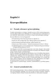
– di direct li linear transformation f i (DLT) 

– error in determination of marker positions 

• Removal of noise in kinematic signals 

– filtering 

– determination of cutoff frequency for filtering 

• Filtering end effects 



- measurement technique and signal processing 

http://www.hst.aau.dk/~mv/ST7_BMsig/ 

Li Literature: 

- Biomechanics of the musculo-skeletal system, 2nd ed. editors Nigg, 

BM and Herzog W, Wiley 1999. 

-Biomechanics Biomechanics and control of mo movement ement 2nd ed ed. D.A. D A Winter Winter, Wiley- Wile 

Inter science Publications 1990 

Web resources: http://www http://www.isbweb.org/ isbweb org/ 

Discussion forum: Biomech-L 


Eadweard Muybridge (1830 – 1904) 

• ‘The father of cinematography’ 

See e.g. http://www.muybridge.nl 


Eadweard dwe d Muybridge uyb dge (1830 ( – 1904) ) 

- Edward Muybridge, English by birth, immigrates to America in 1851. 

In the 1860s he photographs the landscape of the West. In the spring of 

1872 Leland Stanford invites him to photograph his horses. Stanford, set 

on developing the greatest racing stable in the West, uses every 

scientific research to reach his goal. At the time there is disagreement 

about whether or not all feet leave the ground at one time during the 

gallop. 

- In June 1878 six successful series are published on cards as “The 

horse in motion." It clearly shows the different stages of the horse's legs 

during the run, walk, trot and gallop. For this series Muybridge used 12 

cameras and does not use threads but a clockwork to trigger the 

sequence of shutters. 



- Kinematics of 

animal motion 

(parrot) 



- Kinematics of human performance (one legged jump) 


Kinematics e cs – measurement techniques q 

• AAccelerometry l t 

• Potentiometers, flexible wire goniometers 

(angular information alone) 

• Chronocyclography 

• Light emitting diodes 

• St Stroboscopes b 

• Active markers 

• Magnetic systems 

• Motion film cameras and skin marker 

• Video cameras and skin markers 

• Video cameras + reflective skin markers 


Accelerometry 

Mode of operation 

Uni axial – multi axial 


Goniometry 

- Potentiometers (3 degrees of freedom (DOF)) 

- The depicted type require no information about the position the of axes of 

rotations of the joint on which it is mounted 


Goniometry 

- Flexible wire goniometers (2 DOF) 

- strain gauge technology 

The flexible wire 

Embedded electronics 

- htt http://www.biometricsltd.com // bi t i ltd - Cross-section of the flexible wire 

Resistances 

channel 2, 2 half bridge 

wire 

Resistances 

Channel 1, half bridge 


Goniometry + foot switches – an example application 

- Application of flexible wire 

goniometers: 

Measurement of foot kinematics 

- Calcaneal angle in the frontal 

plane 

- Changes in navicular height 

Ref. file : MK030821002 

Data file : MK030821005 

blue line = average of 10 steps 

red line = + +- 1SD 1 SD 

calcaneus, frontal plane NB! for all goniometer channels: 0 = standing 

30 

positive = inversion/supination 

20 

10 

Mean 10.2 

Min -0.1 

Max 23 23.1 1 

+- 0.6 deg 

+- 0.7 deg 

+ +- 22.1 1 deg 

[deg] 

[cm] 

[V] 

0 

Calcaneus reference angle = 0 deg 

-10 

0 

navicular 

10 

heigth g 

20 30 40 50 60 70 80 90 100 

65 

dNavH stance = -3.7+- 0.7 mm 

dNavH total = 9.3 +- 0.4 mm 

mean NavH = 58.3 +- 0.3 mm 

NavH ref = 56 mm 

60 

55 

0 10 20 30 40 50 60 70 80 90 100 

10 footswitch 

8 

6 

4 

2 

Phases: heel,flat heel flat foot, foot forefoot/toe, forefoot/toe swing 

Cyclus time = 962 +- 8 ms 

Step freq = 1.04 +- 0.01 Hz 

Heel = 8 +- 1 % cyclus 

Flatfoot = 25 +- 1 % cyclus 

Forefoot = 57 +- 1 % cyclus 

0 10 20 30 40 50 60 70 80 90 100 

0 

gait cycle [%] 


Chronocyclography 

C o ocyc og p y 

Chronocyclograph (approx. 100 Hz) 

- Shoulder and hand movement 

during gright g hand straight g ppunch 

- light source mounted on the 

shoulder and the hand 

(MV master thesis 1987) 

-setup 

- recording 

max. velocity 


Light g emitting e g diodes d odes 

Weight lifting : clean & jerk technique 

+ flash 2. -flash 

44. 

1. 

55. 

3. 

- Still picture camera with open 

shutter 

- Flash 

- 50 Hz light emitting diodes 

mounted on the end of the 

barbell and on the floor 


Stroboscopes 

S oboscopes 

- for quantitative measurements 

See e.g. 

http://www.elmed-stroboscopes.com/ 

- for illustrative purposes 


Motion o o film cameras c e s – intermittent pin p 

light : 8 kW ! 

16 mm film 500 frs s-1 16 mm film, 500 frs s 


Motion o o film cameras c e s – rotating gpprism 

For high speed cinematography products see e.g. 

http://www http://www.photosonics.com/ 

photosonics com/ 


Motion o o film technology ec o ogy – film digitization g 

Manual: 

- PProjection j ti of f each h picture i t frame f onto t a digitizing di iti i 

tablet and manual digitization (custom made setup) 

Semi automatic: 

- Contrast enhanced field of view 

dduring i the h recording di 

- Frame-by- frame transfer of film to 

video (ElmoTM TRV-166) 

- Automatic tracking in video pictures 

bby PPeak k PPerformance f TTechnologies h l i TM 

motion capture system software 

http://www.peakperform.com 


Magnetic sensors and systems 

11. Th They measure roll, ll pitch it h and d yaw and d X,Y,Z X YZ 

positions of segments 

2. Electromagnetic induction 

3. The transmitter is a triad of electromagnetic g 

coils, that emits the magnetic fields. The 

transmitter is the system’s reference frame. 

4. The receiver is a small triad of 

electromagnetic l t ti coils, il that th t detects d t t the th 

magnetic field emitted by the transmitter and 

the position and orientation is measured as 

the receiver is moved 

Positive: The body is ‘transparent’, real time 

recording 

NNegative: ti Obtrusive, Obt i rather th low l accuracy, 

sensitive to ferro-magnetic objects 

Fasttrack (120 Hz max.) 

h http://www.polhemus.com 

// lh 

Other systems: 

Flock of birds TM 

http://www.ascension-tech.com/ 


Optoelectronic systems 

– with active markers 

Optotrack PolarisTM Optotrack Polaris 

1. Markers consists of light emitting diodes 

(LED’s). ( ) 

2. Up to three marker clusters. 

3. Time multiplexing for the markers 450 Hz 

or 750 Hz. 

44. PPower tto th the markers k is i provided id d through th h 

cables! 

5. No tracking – real time recording 

6. Very yhigh g accuracy y( (0.1 mm X,Y) , ) and 0.15 

mm (Z, depth). http://www.ndidigital.com 

Other (older) systems: 

Watsmart TM 

Selspot II TM 


Video technology 

– with reflective markers and automatic detection 

1. Reflective markers are mounted on the target 

object. 

2. The camera emits infrared (IR) flashes from IR- 

diodes synchronized with the camera shutter. shutter 

3. In each ‘picture frame’ the camera records the 

reflected IR-light from the markers over a period 

determined by the shutter speed. 

4. The picture information is lost and only the bright 

spots corresponding to reflected light from the 

markers are ‘seen’ by the cameras. 

55. The video pictures are digitized. digitized 

6. The firmware in the cameras identifies the bright 

pixel clusters corresponding to the marker 

reflections and calculates the x-y coordinates of 

the centroid. 

7. The 2D camera coordinates are sent to a PC 

through a high speed serial connection. For further 

processing 

ProReflex cameras (1 1000 frs s ) 

- ProReflex cameras (1 – 1000 frs s -1 ) 

http://www.qualisys.se 

Other manufacturers: 

Vicon TM (http://www.oxfordmetrics.com) 

( p ) 

Motion Analysis TM Corp. 

(http://motionanalysis.com) 

Elite TM (http://www.bts.it) 

Peak Performance TechnologiesTM processing. Peak Performance TechnologiesTM (http://www.peakperform.com) 


Determination of marker positions in 3D 

- issues of accuracy 

• Accuracy of the calibration frame 

• Quality of the DLT reconstruction 

• Quality of the lenses 

• Deformation of the film in the image plane 

• Resolution of the light sensitive chip 



- di direct t linear li transformation 

t f ti 

- provides a linear relationship between two dimensional coordinates (x,y) of 

a marker i = (1,…..,m), the cameras (n cameras (1,….,j)) and the coordinates 

on the film and its location in the three dimensional space. 



- direct linear transformation 

- A calibration lib ti of f N points i t with ith known k coordinates di t xr,yr,zr ( (r = 1,….,N) 1 N) iis 

used for determination of coefficients akj for each camera 

- 11 coefficients have to be determined 

- each camera is described by two equations 

- as long as a minimum of two cameras are used 

6 calibration points gives therefore 12 equations 

- the over-determined over determined of system of linear equations is solved by least 

squares technique 

- the solution is not unique since the measurements 

are not perfect and the solution is approximated 

by minimizing errors (∆j) i.e. the ‘norm of residuals’ 

(NR) ( ) defined as: 

(N=12) 


Marker positions 

- potential sources of error 

• Errors implicit in the direct linear 

transformation 



- lens correction 

Correction term in the DLT 

Calc. 



- potential sources of error 

• errors due to relative camera placement 

- cameras should be placed at 

angle near 90o and not less than 

60o 60 


Errors in rigid body motion 

-using i markers k 

- marker movement (skin ( mounted markers) ) 

- errors due to relative marker movement 

(movement of markers in relative to each other) 

- can be solved by using marker attachment systems/frames 


Errors in rigid body motion 

-using i markers k 

- absolute marker movement 

(movement ( of markers in relation 

to anatomical landmarks) 

- can bbe solved l db by using i bone b 

fixed markers 


Using bone mounted markers 

- for more accurate kinematics 

KK-wires i 2 mm diam. di 

Marker cluster 

(19 mm reflective 

markers) 

Insertion pin p 

(tibia, calcaneus) 

Insertion pin 

(navicula) 

90 deg adapter 

(navicula) 

Calcaneus 

PPoint i tof fi insertion ti 

(navicula) - Ready to go 

Local anaesthesia 

(calcaneus) 

X-ray guided insertion 

Insertion depth 20-25 mm 

Tibia 

Navicula 

(Voigt, Christensen and Simonsen XX ISB Conference 2005 ) 

ST7_BM_Meas&Sign MM4,2010 30 

30

Sampling S p g frequency eque cy 


Kinematic e cs signals g s 


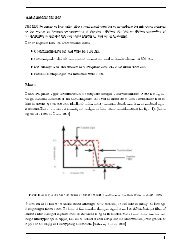
Kinematic e cs signals g s – and noise 


Kinematics e cs – effects of high g frequent q noise 


Kinematic e cs signals g s – smoothing gtechniques q 

e.g. 

• least squares polynomial fitting 

• spline interpolation 

• filtering 


Kinematics e cs – smoothing gtechniques q 


Kinematic e cs signals g s – filtering gand cut off frequency q y 



• for most applications a 2nd order digital Butterworth filter, 

performed f d bidirectionally bidi i ll has h proven to be b adequate. d The Th procedure d 

gives a ’zerolag 4th order Butterworth filter’ 



• determination of the cutoff frequency for the filter 

– Frequency analysis (Fast Fourier Transform) 

– A residual analysis 

filtering frequency 


Kinematics e cs – calculation of velocity y and acceleration 

- velocity 

- acceleration 

or 


Segment Seg e and d Jo Joint angles g es – 2D 

Segment angles: 

- in relation to horizontal 

- counter clockwise = positive 

Joint angles: e.g. 


Opgaver pg 

1. Signalfil : DJ_toe_marker.txt, en manuelt digitaliseret 2D-koordinat (i m) af 5. metatarsalled 

filmet med mekanisk filmkamera med 500 Hz i sagittalplanet. 

- implementer en Matlab-funktion, der filtrerer med et 4. ordens Butterworth filter med en cut off 

frekvens på 6 Hz og g plot signalet g for den filtrerede y-koordinat y ovenpå det rå signal g for samme 

koordinat. Bemærk forskellen mellem det rå og det filtrerede signal i ved slutningen af signalet 

for y-koordinaten. Hvad skyldes denne forskel. 

- Lav en Matlab – rutine der løser dette problem med ’end effects’. 

- Giv et kvalificeret bud på hvilken cutoff frekvens, der skal bruges til filtrering af signalerne for 

hhv hhv. x og y koordinaterne 

koordinaterne. 

- Hvorledes vil du afgøre om de cutoff frekvenser du har valgt er i orden m.h.t. til videre 

kinematisk analyse? 

2. Signalfil g : kdat.mat, , 3D-koordinater af markører ø på p venstre ben under et fodboldspark p (optaget ( p g med 

ProReflex med 240 Hz, angivet i mm). (m-fil (kick_input.m) medfølger med beskrivelse af 

koordinaterne i datafilen (kin_dat.mat). XZ-planet svarer til sagittal planet. Signalerne er ikke 

filtrerede. 

- forsøg at tegne et såkaldt stick-diagram af bevægelse for at visualisere bevægelsen, der sparkes 

fra venstre måde højre) 

- beregn knævinklen i xz planet og udtryk den som anatomisk vinkel (0 grader er strakt ben og 

fleksion er positiv) 

- beregn hoftevinklen i xz- planet og udtryk den som anatomisk vinkel (0 grader er strakt ben og 

fleksion er 

- beregn knævinkel- og hoftevinkelhastigheder og plot dem i samme koordinatststem som 

funktion af tiden 

- Hvilke problemer kan der opstå når en hastighed beregnes simpelt med finite differences ( (x 1x 

2)/dt )? 

Data findes på http://www.hst.aau.dk/~mv/ST7_BMsig/Litt

ST7 Biomechanics

Create successful ePaper yourself

Delete template?

Save as template?