Lecture 7 ? Summary and Applications of JTFA From the ...
Lecture 7 ? Summary and Applications of JTFA From the ...
Lecture 7 ? Summary and Applications of JTFA From the ...

Create successful ePaper yourself
Turn your PDF publications into a flip-book with our unique Google optimized e-Paper software.
<strong>Lecture</strong> 7<br />
<strong>Summary</strong> <strong>and</strong> <strong>Applications</strong> <strong>of</strong><br />
Joint Time-Frequency Analysis<br />
Time-frequency analysis, adaptive<br />
filtering <strong>and</strong> source separation<br />
José Biurrun Manresa<br />
22.03.2011
• <strong>Summary</strong> <strong>of</strong> <strong>JTFA</strong><br />
<strong>Lecture</strong> 7 – <strong>Summary</strong> <strong>and</strong> <strong>Applications</strong> <strong>of</strong> <strong>JTFA</strong><br />
Overview<br />
• Short Time Fourier Transform<br />
• Wigner-Ville distribution<br />
• Kernel properties <strong>and</strong> design in Cohen’s class time-frequency<br />
distributions<br />
• Biomedical applications <strong>of</strong> <strong>JTFA</strong><br />
2
<strong>Lecture</strong> 7 – <strong>Summary</strong> <strong>and</strong> <strong>Applications</strong> <strong>of</strong> <strong>JTFA</strong><br />
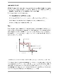
What <strong>the</strong> Fourier transform misses...<br />
3
<strong>Lecture</strong> 7 – <strong>Summary</strong> <strong>and</strong> <strong>Applications</strong> <strong>of</strong> <strong>JTFA</strong><br />
Timing is also important!<br />
• For many signals, it is not enough to know <strong>the</strong> global frequecy<br />
content<br />
• We also need to know <strong>the</strong> timing in which <strong>the</strong>se changes in<br />
frequency occurr, in order to follow <strong>the</strong> dynamics <strong>of</strong> <strong>the</strong> signal<br />
• Which signals are <strong>the</strong>se?<br />
• Non-stationary, transient, whose parameters change with time<br />
(derived from a non-LTI system)<br />
4
<strong>Lecture</strong> 7 – <strong>Summary</strong> <strong>and</strong> <strong>Applications</strong> <strong>of</strong> <strong>JTFA</strong><br />
Some toy examples...<br />
5
<strong>Lecture</strong> 7 – <strong>Summary</strong> <strong>and</strong> <strong>Applications</strong> <strong>of</strong> <strong>JTFA</strong><br />
... And some real examples<br />
6
<strong>Lecture</strong> 7 – <strong>Summary</strong> <strong>and</strong> <strong>Applications</strong> <strong>of</strong> <strong>JTFA</strong><br />
... And some real examples<br />
7
<strong>Lecture</strong> 7 – <strong>Summary</strong> <strong>and</strong> <strong>Applications</strong> <strong>of</strong> <strong>JTFA</strong><br />
... And some real examples<br />
8
<strong>Lecture</strong> 7 – <strong>Summary</strong> <strong>and</strong> <strong>Applications</strong> <strong>of</strong> <strong>JTFA</strong><br />
Analyze by segments using <strong>the</strong> FT<br />
9
<strong>Lecture</strong> 7 – <strong>Summary</strong> <strong>and</strong> <strong>Applications</strong> <strong>of</strong> <strong>JTFA</strong><br />
Short-Time Fourier Transform (STFT)<br />
• Basic approach: slicing <strong>the</strong> wavefor <strong>of</strong> interest into a number<br />
<strong>of</strong> short segments <strong>and</strong> performing <strong>the</strong> Fourier transform on<br />
each one <strong>of</strong> <strong>the</strong>m<br />
• A window function is applied to a segment <strong>of</strong> <strong>the</strong> signal, thus<br />
isolating it from <strong>the</strong> overall waveform<br />
<br />
10
<strong>Lecture</strong> 7 – <strong>Summary</strong> <strong>and</strong> <strong>Applications</strong> <strong>of</strong> <strong>JTFA</strong><br />
Short-Time Fourier Transform (STFT)<br />
• Since <strong>the</strong> modified signal emphasizes <strong>the</strong> original signal around<br />
<strong>the</strong> time , <strong>the</strong> Fourier transform will reflect <strong>the</strong> distribution<br />
<strong>of</strong> frequencies around that time<br />
1<br />
1<br />
2 <br />
2 <br />
11
<strong>Lecture</strong> 7 – <strong>Summary</strong> <strong>and</strong> <strong>Applications</strong> <strong>of</strong> <strong>JTFA</strong><br />
Short-Time Fourier Transform (STFT)<br />
12
<strong>Lecture</strong> 7 – <strong>Summary</strong> <strong>and</strong> <strong>Applications</strong> <strong>of</strong> <strong>JTFA</strong><br />
Short-Time Fourier Transform (STFT)<br />
• The energy density spectrum at time is<br />
, 1<br />
2 <br />
• For each different time we get a different spectrum, <strong>and</strong> <strong>the</strong><br />
totality <strong>of</strong> <strong>the</strong>se spectra is <strong>the</strong> time-frequency distribution .<br />
• The most common name for this distribution is spectrogram<br />
<br />
13
<strong>Lecture</strong> 7 – <strong>Summary</strong> <strong>and</strong> <strong>Applications</strong> <strong>of</strong> <strong>JTFA</strong><br />
Spectrogram<br />
14
<strong>Lecture</strong> 7 – <strong>Summary</strong> <strong>and</strong> <strong>Applications</strong> <strong>of</strong> <strong>JTFA</strong><br />
Spectrogram<br />
• Ano<strong>the</strong>r way to look at it is as a change <strong>of</strong> <strong>the</strong> function basis<br />
Fourier<br />
Transform<br />
STFT<br />
Narrowb<strong>and</strong><br />
STFT<br />
Wideb<strong>and</strong><br />
15
<strong>Lecture</strong> 7 – <strong>Summary</strong> <strong>and</strong> <strong>Applications</strong> <strong>of</strong> <strong>JTFA</strong><br />
Uncertainty principle<br />
16
<strong>Lecture</strong> 7 – <strong>Summary</strong> <strong>and</strong> <strong>Applications</strong> <strong>of</strong> <strong>JTFA</strong><br />
Uncertainty principle<br />
• We cannot simultaneously know time <strong>and</strong> frequency aspects<br />
<strong>of</strong> a signal at an arbitrary resolution<br />
• For each value <strong>of</strong> <strong>and</strong> , <strong>the</strong>re is a rectangle whose sides are<br />
determined by <strong>and</strong> , <strong>and</strong> whose area is at least ⁄ <br />
• When <strong>the</strong> window is selected, <strong>the</strong> resolution is fixed in<br />
time <strong>and</strong> frequency<br />
• Since <strong>the</strong> window is always equal <strong>and</strong> just shifts in time,<br />
<strong>the</strong> STFT has an uniform resolution both in time <strong>and</strong><br />
frequency<br />
17
<strong>Lecture</strong> 7 – <strong>Summary</strong> <strong>and</strong> <strong>Applications</strong> <strong>of</strong> <strong>JTFA</strong><br />
Uncertainty principle<br />
18
Frequency<br />
<strong>Lecture</strong> 7 – <strong>Summary</strong> <strong>and</strong> <strong>Applications</strong> <strong>of</strong> <strong>JTFA</strong><br />
Uncertainty principle<br />
Time<br />
19
<strong>Lecture</strong> 7 – <strong>Summary</strong> <strong>and</strong> <strong>Applications</strong> <strong>of</strong> <strong>JTFA</strong><br />
Time-Frequency representations<br />
• The Short-Time Fourier Transform (STFT) takes a linear<br />
approach for a time-frequency representation<br />
• It decomposes <strong>the</strong> signal on elementary components, called<br />
atoms<br />
, <br />
• Each atom is obtained from <strong>the</strong> window by a translation<br />
in time <strong>and</strong> a translation in frequency (modulation)<br />
20
<strong>Lecture</strong> 7 – <strong>Summary</strong> <strong>and</strong> <strong>Applications</strong> <strong>of</strong> <strong>JTFA</strong><br />
Time-Frequency representations<br />
• If we consider <strong>the</strong> square modulus <strong>of</strong> <strong>the</strong> STFT, we get <strong>the</strong><br />
spectrogram, which is th spectral energy density <strong>of</strong> <strong>the</strong><br />
locally windowed signal <br />
• The spectrogram is a quadratic or bilinear representation<br />
• If <strong>the</strong> energy <strong>of</strong> <strong>the</strong> windows is selected to be one, <strong>the</strong> energy<br />
<strong>of</strong> <strong>the</strong> spectrogram is equal to <strong>the</strong> energy <strong>of</strong> <strong>the</strong> signal<br />
• Thus, it can be interpreted as a measure <strong>of</strong> <strong>the</strong> energy <strong>of</strong> <strong>the</strong><br />
signal contained in <strong>the</strong> time-frequency domain centered on <strong>the</strong><br />
point , <br />
21
• Linear<br />
• STFT<br />
• Wavelet<br />
<strong>Lecture</strong> 7 – <strong>Summary</strong> <strong>and</strong> <strong>Applications</strong> <strong>of</strong> <strong>JTFA</strong><br />
Time-Frequency representations<br />
• Bilinear or Quadratic<br />
• Cohen’s class<br />
• Spectrogram<br />
• Wigner-Ville<br />
• Choi-Williams<br />
• ...<br />
• Affine distributions<br />
22
<strong>Lecture</strong> 7 – <strong>Summary</strong> <strong>and</strong> <strong>Applications</strong> <strong>of</strong> <strong>JTFA</strong><br />
The Wigner-Ville Distribution<br />
• The Wigner-Ville (<strong>and</strong> all <strong>of</strong> Cohen’s class <strong>of</strong> distribution) uses<br />
a variation <strong>of</strong> <strong>the</strong> autocorrelation function wher time remains<br />
in <strong>the</strong> result, called instantaneous autocorrelation<br />
function<br />
, 2 ∗ 2 <br />
Where is <strong>the</strong> time lag <strong>and</strong> ∗ represents <strong>the</strong> complex conjugate<br />
<strong>of</strong> <strong>the</strong> signal .<br />
23
<strong>Lecture</strong> 7 – <strong>Summary</strong> <strong>and</strong> <strong>Applications</strong> <strong>of</strong> <strong>JTFA</strong><br />
The Wigner-Ville Distribution<br />
• Instantaneous autocorrelation <strong>of</strong> four cycle sine plots<br />
24
<strong>Lecture</strong> 7 – <strong>Summary</strong> <strong>and</strong> <strong>Applications</strong> <strong>of</strong> <strong>JTFA</strong><br />
The Wigner-Ville Distribution<br />
• The Wigner-Ville Distribution (WVD) is defined as<br />
or equivalently<br />
, 1<br />
2 2 ∗ 2 , 1<br />
2 2<br />
∗ 2<br />
25
<strong>Lecture</strong> 7 – <strong>Summary</strong> <strong>and</strong> <strong>Applications</strong> <strong>of</strong> <strong>JTFA</strong><br />
The Wigner-Ville Distribution<br />
26
<strong>Lecture</strong> 7 – <strong>Summary</strong> <strong>and</strong> <strong>Applications</strong> <strong>of</strong> <strong>JTFA</strong><br />
The Wigner-Ville Distribution<br />
• In an analogy to <strong>the</strong> STFT, <strong>the</strong> window is basically a shifted<br />
version <strong>of</strong> <strong>the</strong> same signal<br />
• It is obtained by comparing <strong>the</strong> information <strong>of</strong> <strong>the</strong> signal with<br />
its own information at o<strong>the</strong>r times <strong>and</strong> frequencies<br />
• It possesses several interesting properties!<br />
27
<strong>Lecture</strong> 7 – <strong>Summary</strong> <strong>and</strong> <strong>Applications</strong> <strong>of</strong> <strong>JTFA</strong><br />
Properties <strong>of</strong> <strong>the</strong> WVD<br />
• Energy conservation<br />
• Real-valued<br />
• Marginal properties<br />
• Translation <strong>and</strong> dilation covariance<br />
• Compatibility with filterings<br />
• Wide-sense support conservation<br />
• Unitarity<br />
28
<strong>Lecture</strong> 7 – <strong>Summary</strong> <strong>and</strong> <strong>Applications</strong> <strong>of</strong> <strong>JTFA</strong><br />
Interference in <strong>the</strong> WVD<br />
• As <strong>the</strong> WVD is a bilinear function <strong>of</strong> <strong>the</strong> signal , <strong>the</strong> quadratic<br />
superposition principle applies<br />
where<br />
, , , 2 , , <br />
, , 1<br />
2 2 ∗ 2 is <strong>the</strong> cross-WVD <strong>of</strong> <strong>and</strong> <br />
29
<strong>Lecture</strong> 7 – <strong>Summary</strong> <strong>and</strong> <strong>Applications</strong> <strong>of</strong> <strong>JTFA</strong><br />
Interference in <strong>the</strong> WVD<br />
30
<strong>Lecture</strong> 7 – <strong>Summary</strong> <strong>and</strong> <strong>Applications</strong> <strong>of</strong> <strong>JTFA</strong><br />
Interference in <strong>the</strong> WVD<br />
31
<strong>Lecture</strong> 7 – <strong>Summary</strong> <strong>and</strong> <strong>Applications</strong> <strong>of</strong> <strong>JTFA</strong><br />
Interference in <strong>the</strong> WVD<br />
32
<strong>Lecture</strong> 7 – <strong>Summary</strong> <strong>and</strong> <strong>Applications</strong> <strong>of</strong> <strong>JTFA</strong><br />
Interference in <strong>the</strong> WVD<br />
• These interference terms are troublesome since <strong>the</strong>y may<br />
overlap with auto-terms (signal terms) <strong>and</strong> thus make it<br />
difficult to visually interpret <strong>the</strong> WVD image.<br />
• It appears that <strong>the</strong>se terms must be present or <strong>the</strong> good<br />
properties <strong>of</strong> <strong>the</strong> WVD (marginal properties, instantaneous<br />
frequency <strong>and</strong> group delay, localization, unitarity . . . ) cannot<br />
be satisfied<br />
• There is a trade-<strong>of</strong>f between <strong>the</strong> quantity <strong>of</strong> interferences <strong>and</strong><br />
<strong>the</strong> number <strong>of</strong> good properties<br />
33
<strong>Lecture</strong> 7 – <strong>Summary</strong> <strong>and</strong> <strong>Applications</strong> <strong>of</strong> <strong>JTFA</strong><br />
Pseudo-WVD<br />
• The definition <strong>of</strong> <strong>the</strong> WVD requires <strong>the</strong> knowledge <strong>of</strong><br />
, 2 ∗ 2 <br />
from ∞ to ∞, which can be a problem in practice<br />
• Often a windowed version <strong>of</strong> , is used, leading to <strong>the</strong><br />
Pseudo-WVD (PWVD)<br />
, 1<br />
2 2 ∗ 2 34
<strong>Lecture</strong> 7 – <strong>Summary</strong> <strong>and</strong> <strong>Applications</strong> <strong>of</strong> <strong>JTFA</strong><br />
Pseudo-WVD<br />
35
<strong>Lecture</strong> 7 – <strong>Summary</strong> <strong>and</strong> <strong>Applications</strong> <strong>of</strong> <strong>JTFA</strong><br />
Pseudo-WVD<br />
• However, <strong>the</strong> consequence <strong>of</strong> this improved readability is that<br />
many properties <strong>of</strong> <strong>the</strong> WVD are lost:<br />
• The marginal properties<br />
• The unitarity<br />
• The frequency-support conservation<br />
• The frequency-widths <strong>of</strong> <strong>the</strong> auto-terms are increased by this<br />
operation<br />
36
<strong>Lecture</strong> 7 – <strong>Summary</strong> <strong>and</strong> <strong>Applications</strong> <strong>of</strong> <strong>JTFA</strong><br />
Relationship between <strong>the</strong> WVD <strong>and</strong> <strong>the</strong><br />
spectrogram<br />
• The spectrogram can be expressed as a smoothing <strong>of</strong> <strong>the</strong> WVD<br />
, 1<br />
2 <br />
<br />
, , <br />
• The smoothing function Φ , , is controlled only<br />
by <strong>the</strong> short-time window <br />
• We can add ano<strong>the</strong>r degree <strong>of</strong> freedom Φ , <br />
allowing a progressive, independent control in both time <strong>and</strong><br />
frequency <strong>of</strong> <strong>the</strong> smoothing applied to <strong>the</strong> WVD<br />
37
<strong>Lecture</strong> 7 – <strong>Summary</strong> <strong>and</strong> <strong>Applications</strong> <strong>of</strong> <strong>JTFA</strong><br />
Variations <strong>of</strong> WVD<br />
WVD PWVD SPWVD<br />
38
<strong>Lecture</strong> 7 – <strong>Summary</strong> <strong>and</strong> <strong>Applications</strong> <strong>of</strong> <strong>JTFA</strong><br />
<strong>From</strong> <strong>the</strong> spectrogram to <strong>the</strong> WVD<br />
39
<strong>Lecture</strong> 7 – <strong>Summary</strong> <strong>and</strong> <strong>Applications</strong> <strong>of</strong> <strong>JTFA</strong><br />
The ambiguity function<br />
• The symmetrical ambiguity function (AF)<br />
, 2 ∗ 2 • The AF is a measure <strong>of</strong> <strong>the</strong> time-frequency correlation <strong>of</strong> <strong>the</strong><br />
signal <br />
• The ambiguity function is <strong>the</strong> 2-D Fourier transform <strong>of</strong> <strong>the</strong><br />
WVD. Consequently for <strong>the</strong> AF, a dual property corresponds<br />
to nearly all <strong>the</strong> properties <strong>of</strong> <strong>the</strong> WVD<br />
40
<strong>Lecture</strong> 7 – <strong>Summary</strong> <strong>and</strong> <strong>Applications</strong> <strong>of</strong> <strong>JTFA</strong><br />
Properties <strong>of</strong> <strong>the</strong> AF<br />
41
<strong>Lecture</strong> 7 – <strong>Summary</strong> <strong>and</strong> <strong>Applications</strong> <strong>of</strong> <strong>JTFA</strong><br />
Properties <strong>of</strong> <strong>the</strong> AF<br />
42
<strong>Lecture</strong> 7 – <strong>Summary</strong> <strong>and</strong> <strong>Applications</strong> <strong>of</strong> <strong>JTFA</strong><br />
Cohen’s class<br />
• The approach characterizes time-frequency distributions by an<br />
auxiliary function called <strong>the</strong> kernel function<br />
• The properties <strong>of</strong> a particular distribution are reflected by<br />
simple constraints on <strong>the</strong> kernel<br />
• Therefore, it is possible to choose those kernels with<br />
prescribed, desirable properties<br />
• This general class can be described in a number <strong>of</strong> different<br />
ways<br />
43
<strong>Lecture</strong> 7 – <strong>Summary</strong> <strong>and</strong> <strong>Applications</strong> <strong>of</strong> <strong>JTFA</strong><br />
General description <strong>of</strong> Cohen’s class<br />
• All time-frequency representations can be obtained from<br />
, 1<br />
4 , 2 ∗ 2 or equivalently<br />
, 1<br />
4 , ∗ 2<br />
2<br />
where , is <strong>the</strong> kernel function<br />
44
<strong>Lecture</strong> 7 – <strong>Summary</strong> <strong>and</strong> <strong>Applications</strong> <strong>of</strong> <strong>JTFA</strong><br />
General description <strong>of</strong> Cohen’s class<br />
45
<strong>Lecture</strong> 7 – <strong>Summary</strong> <strong>and</strong> <strong>Applications</strong> <strong>of</strong> <strong>JTFA</strong><br />
O<strong>the</strong>r important energy distributions<br />
• The Rihaczek distribution<br />
• The Margenau-Hill distribution<br />
• The Page distribution<br />
46
<strong>Lecture</strong> 7 – <strong>Summary</strong> <strong>and</strong> <strong>Applications</strong> <strong>of</strong> <strong>JTFA</strong><br />
O<strong>the</strong>r important energy distributions<br />
• Joint-smoothings <strong>of</strong> <strong>the</strong> WVD: <strong>the</strong> following distributions<br />
correspond to particular cases <strong>of</strong> <strong>the</strong> Cohen’s class for which<br />
<strong>the</strong> parameterization function depends only on <strong>the</strong> product <strong>of</strong><br />
<strong>the</strong> variables <strong>and</strong> <br />
, <br />
where is a decreasing function such that 0 1<br />
• A direct consequence <strong>of</strong> this definition is that <strong>the</strong> marginal<br />
properties will be respected<br />
47
<strong>Lecture</strong> 7 – <strong>Summary</strong> <strong>and</strong> <strong>Applications</strong> <strong>of</strong> <strong>JTFA</strong><br />
O<strong>the</strong>r important energy distributions<br />
• Since is a decreasing function, is a low-pass function, <strong>and</strong><br />
thus, this parameterization function will reduce <strong>the</strong><br />
interferences.<br />
• That is why <strong>the</strong>se distributions are also known as <strong>the</strong> Reduced<br />
Interference Distributions (RID)<br />
• Some examples are: Choi-Williams, Born-Jordan <strong>and</strong><br />
Zhao-Atlas-Marks distributions<br />
48
<strong>Lecture</strong> 7 – <strong>Summary</strong> <strong>and</strong> <strong>Applications</strong> <strong>of</strong> <strong>JTFA</strong><br />
O<strong>the</strong>r important energy distributions<br />
49
<strong>Lecture</strong> 7 – <strong>Summary</strong> <strong>and</strong> <strong>Applications</strong> <strong>of</strong> <strong>JTFA</strong><br />
O<strong>the</strong>r important energy distributions<br />
50
<strong>Lecture</strong> 7 – <strong>Summary</strong> <strong>and</strong> <strong>Applications</strong> <strong>of</strong> <strong>JTFA</strong><br />
O<strong>the</strong>r important energy distributions<br />
51
<strong>Lecture</strong> 7 – <strong>Summary</strong> <strong>and</strong> <strong>Applications</strong> <strong>of</strong> <strong>JTFA</strong><br />
<strong>Summary</strong><br />
• The Cohen’s class ga<strong>the</strong>r all <strong>the</strong> quadratic time-frequency<br />
distributions covariant by shifts in time <strong>and</strong> in frequency<br />
• It <strong>of</strong>fers a wide set <strong>of</strong> powerful tools to analyze non-stationary<br />
signals. The basic idea is to devise a joint function <strong>of</strong> time <strong>and</strong><br />
frequency that describes <strong>the</strong> energy density or intensity <strong>of</strong> a<br />
signal simultaneously in time <strong>and</strong> in frequency<br />
• The most important element <strong>of</strong> this class is probably <strong>the</strong><br />
Wigner-Ville distribution, which satisfies many desirable<br />
properties<br />
52
<strong>Lecture</strong> 7 – <strong>Summary</strong> <strong>and</strong> <strong>Applications</strong> <strong>of</strong> <strong>JTFA</strong><br />
<strong>Summary</strong><br />
• Since <strong>the</strong>se distributions are quadratic, <strong>the</strong>y introduce crossterms<br />
in <strong>the</strong> time-frequency plane which can disturb <strong>the</strong><br />
readability <strong>of</strong> <strong>the</strong> representation<br />
• One way to attenuate <strong>the</strong>se interferences is to smooth <strong>the</strong><br />
distribution in time <strong>and</strong> in frequency, according to <strong>the</strong>ir<br />
structure<br />
• The consequence <strong>of</strong> this is a decrease <strong>of</strong> <strong>the</strong> time <strong>and</strong><br />
frequency resolutions, <strong>and</strong> more generally a loss <strong>of</strong> <strong>the</strong>oretical<br />
properties<br />
53
<strong>Lecture</strong> 7 – <strong>Summary</strong> <strong>and</strong> <strong>Applications</strong> <strong>of</strong> <strong>JTFA</strong><br />
References <strong>and</strong> fur<strong>the</strong>r reading<br />
• Time Frequency Analysis: Theory <strong>and</strong> <strong>Applications</strong> by Leon<br />
Cohen. Prentice Hall; 1994.<br />
• Biosignal <strong>and</strong> Medical Image Processing, Second Edition by<br />
John L. Semmlow. CRC press; 2009.<br />
• The Time Frequency Toolbox tutorial<br />
(http://tftb.nongnu.org/tutorial.pdf)<br />
• Slides from <strong>JTFA</strong> course by Dario Farina<br />
54
<strong>Lecture</strong> 7 – <strong>Summary</strong> <strong>and</strong> <strong>Applications</strong> <strong>of</strong> <strong>JTFA</strong><br />
<strong>Applications</strong>: Time Frequency Distribution <strong>of</strong><br />
Cardiac Sounds<br />
55
<strong>Lecture</strong> 7 – <strong>Summary</strong> <strong>and</strong> <strong>Applications</strong> <strong>of</strong> <strong>JTFA</strong><br />
<strong>Applications</strong>: Spectrograms <strong>of</strong> EEG signals from<br />
<strong>the</strong> cortex <strong>of</strong> <strong>the</strong> rat<br />
56
<strong>Lecture</strong> 7 – <strong>Summary</strong> <strong>and</strong> <strong>Applications</strong> <strong>of</strong> <strong>JTFA</strong><br />
<strong>Applications</strong>: Fatigue assessment using WVD <strong>of</strong><br />
surface EMG<br />
57
<strong>Lecture</strong> 7 – <strong>Summary</strong> <strong>and</strong> <strong>Applications</strong> <strong>of</strong> <strong>JTFA</strong><br />
<strong>Applications</strong>: Choi-Williams distribution applied<br />
to a burst <strong>of</strong> surface EMG<br />
58
<strong>Lecture</strong> 7 – <strong>Summary</strong> <strong>and</strong> <strong>Applications</strong> <strong>of</strong> <strong>JTFA</strong><br />
<strong>Applications</strong> <strong>of</strong> <strong>JTFA</strong> to biomedical signal<br />
analysis<br />
• Automatic detection <strong>of</strong> conduction block based on time-frequency<br />
analysis <strong>of</strong> unipolar electrograms<br />
• Time-frequency analysis <strong>of</strong> movement-related spectral power in<br />
EEG during repetitive movements: a comparison <strong>of</strong> methods<br />
• Adaptive time-frequency analysis <strong>of</strong> knee joint vibroarthrographic<br />
signals for noninvasive screening <strong>of</strong> articular cartilage pathology<br />
• Instantaneous parameter estimation in cardiovascular time series<br />
by harmonic <strong>and</strong> time-frequency analysis<br />
59