Visualization Systems for Multi-Dimensional Microscopy ... - Springer

14
Visualization Systems for Multi-Dimensional
Microscopy Images
N.S. White
INTRODUCTION
Rapid developments in biological microscopy have prompted
many advances in multi-dimensional imaging. However, threedimensional
(3D) visualization techniques originated largely from
applications involving computer-generated models of macroscopic
objects. Subsequently, these methods have been adapted for biological
visualization of mainly tomographic medical images and
data from cut serial sections (e.g., Cookson et al., 1989 and review
in Cookson, 1994). Most of these algorithms were not devised
specifically for microscopy images, and only a few critical assessments
have been made of suitable approaches for the most
common 3D technique, laser-scanning microscopy (LSM) (Kriete
and Pepping, 1992). Ultimately, we must rely on objective visualization
of control, calibration, and test specimens in order to
determine which visualization algorithms are appropriate for a
particular analysis. Hardware developments and advances in software
engineering tools have made available many 3D reconstruction
systems that can be used to visualize multi-dimensional
images. These are available from instrument manufacturers, third
party vendors, research academics, and other microscopists. The
author has attempted to collate important techniques used in these
programs and to highlight particular packages that, not exclusively,
illustrate various techniques described throughout the text. A representative
collection of established commercial and noncommercial
visualization programs available at the time of writing
is listed in Table 14.1. For automatic image analysis and measurement,
see Chapters 15 and 48, this volume.
The information presented in this chapter about the various
programs is not the result of exhaustive tests or benchmarks but is
merely an overall view of some key issues. The speed of changes
and the rapid appearance (and loss) of particular programs and
hardware from common use make it necessary to concentrate on
important techniques and milestones rather than intricate details of
each package.
Multi-dimensional microscopy data can also be obtained from
instruments other than LSM configurations, such as non-laser confocal
devices and widefield (conventional) systems combined with
image restoration. Although the multi-dimensional data from different
instruments may have different characteristics, the same
basic visualization methods can be used to process the data.
Definitions
A consistent terminology is required to discuss components of
any visualization system, maintaining a fundamental separation
N.S. White • University of Oxford, Oxford OX1 3RE, United Kingdom
between (1) raw images and subsequent processed stages, (2) data
values and the sampled space over which they extend, and (3) final
results and the presentation form of those results. The author prefers
the following terminology: Original intensities from the microscope
comprise an image. Subsequent visualization steps produce
a view. Intensities in an image or view represent the data values,
and the sampling space over which they extend constitutes the
dimensions of the data. Values presented on a screen, hard copy,
etc., are display views. Visualization is the overall process by
which a multi-dimensional display view is made from a biological
specimen, although we will only be concerned with the software
component of this in the present text. Reconstruction refers to the
piecing together of optical sections into a representation of the
specimen object. Rendering is a computer graphics term that
describes the drawing of reconstructed objects into a display view.
What Is the Microscopist Trying to Achieve?
Human visual perception and cognition are highly adapted to interpret
views of large-scale (macroscopic) objects. The human eye
captures low numerical aperture (NA) views like photographic
images. We get information from such views by calling (largely
subconsciously) on a priori information about both the object and
imaging system. High-NA microscope objectives produce images
from which we generate views with properties that we are less
equipped to interpret, for example, the apparent transparency of
most biological samples. This arises from two main processes: (1)
Samples are mostly thin, non-absorbing, and scatter only some of
the illuminating light. Reduced out-of-focus blur, together with
this real transparency enable the confocal and multi-photon LSMs
to probe deep into intact specimens. (2) A high-NA microscope
objective collects light from a large solid angle and can see around
small opaque structures that would otherwise obscure or shadow
details further into the sample. Such intrinsic properties in the
resultant images must be sympathetically handled by an appropriate
visualization system.
The goal of visualization is the formation of easily interpreted
and, sometimes, realistic-looking display views. While pursuing
these aims, several conflicts arise: (1) avoiding visualization artifacts
from inappropriate a priori knowledge, (2) enhancing
selected features of interest, and (3) retaining quantitative information.
Maintaining these goals ensures that the final view can be
used to help obtain unbiased measurements or to draw unambiguous
conclusions. The microscopist must be constantly vigilant
to avoid unreasonably distorting the structural (and intensity)
information in the original image data by over-zealous use of
image processing.
280 Handbook of Biological Confocal Microscopy, Third Edition, edited by James B. Pawley, Springer Science+Business Media, LLC, New York, 2006.

Criteria for Choosing a Visualization System
Assessing any visualization system requires a judgment of (1) features,
(2) usability or friendliness, (3) price/performance, (4) suitability
of algorithms, (5) integration with existing systems, and (6)
validation and documentation of methods or algorithms. The only
way to determine ease of use is by testing the system with typical
users and representative data. The best demonstration images
saved at a facility should never be used to assess a visualization
system for purchase! The host institution’s user profile will help
to formulate more specific questions: What is the purpose of the
reconstructed views? What image information can be represented
in the display views? How must the image data be organized? Are
semi-automated or script-processing (programming) tools available
for preprocessing and can the procedures be adequately tested
and tracked?
WHY DO WE WANT TO VISUALIZE
MULTI-DIMENSIONAL LASER-SCANNING
MICROSCOPY DATA?
The principle uses of a visualization package are to generate subregion
or composite reconstructions from multi-dimensional
images (Fig. 14.1). To collect such views directly from the microscope
is a time-consuming and inefficient process.
There are many advantages to interactively viewing multidimensional
confocal images away from the microscope:
• Damage to the sample by the illumination is reduced.
• Sample throughput on a heavily used system is improved.
• Optimal equipment for data presentation and analysis can be
employed. Serial two-dimensional (2D) orthogonal sections
(e.g., xy, xz, yz, xt, etc.) must be extracted from a 3D/fourdimensional
(4D) image interactively at speeds adequate for
smooth animation. An animation of confocal sections corresponds
to a digital focal series without contrast-degrading blur.
Oblique sections overcome the serial section bias of all confocal
instruments and their smooth, interactive animation is
desirable.
• Reconstructed views are essential to conveniently display a 3D
(Drebin et al., 1988; Robb, 1990) or 4D image (Kriete and
Pepping, 1992) on a 2D display device. The reconstructed
volume may show features that are not discernible when animating
sequential sections (Cookson et al., 1993; Foley et al.,
1990). Reconstructions further reduce the orientationally
biased view obtained from serial sections alone.
• Multiple views are a useful way of extending the dimensional
limitations of the 2D display device. Montages of views make
more efficient use of the pixel display area. Animations make
effective use of the display bandwidth. Intelligent use of color
can further add to our understanding of the information in a
display view (e.g., Boyde, 1992; Kriete and Pepping, 1992;
Masters, 1992).
• For multiple-channel images, flexibility and interactive control
are essential. Multiple channels may require complex color
merging and processing in order to independently control the
visualization of each component.
Data and Dimensional Reduction
Simplification of a complex multi-dimensional image to a 2D
display view implies an important side effect — data and dimen-
Visualization Systems for Multi-Dimensional Microscopy Images • Chapter 14 281
sional reduction. If the required information can be retained in a
display view, substantial improvements in storage space and image
transfer times are possible. This is increasingly important when
presentation results must be disseminated via the Internet (now a
routine option for medical imaging packages such as those from
Cedara and Vital Images Inc.). Data reduction is most obvious in
the case of a single (2D) view of a 3D volume or multiple-channel
image but is actually more significant when 4D data can be distilled
into a series of 2D views (Volocity, Imaris, and Amira, among
other packages, can now seamlessly visualize multi-channel 4D
images). Significant reduction can also be achieved when a single
3D volume of voxels can be represented by a smaller number of
geometric objects. To combine data reduction with quantitative
analyses, a precise description of the object extraction algorithm
must be recorded along with the view; only then can the user determine
the significance of extracted features.
Objective or Subjective Visualization?
The conflict between realistic display and objective reconstruction
persists throughout the visualization process. All of the important
information must be retained in a well-defined framework, defined
by the chosen visualization model or algorithm. Recording of the
parameters at every stage in the visualization is essential. This can
be consistent with the production of convincing or realistic
displays, provided enhancement parameters are clearly described
and can be called upon during the interpretation phase. Multidimensional
image editing must be faithfully logged in order to
relate subregions, even those with expansion or zooming, back to
their original context. Object extraction is a one-way operation that
discards any original image data that falls outside the segmentation
limits. To interpret a reconstruction based on graphically drawn surfaces
we will need to refer back to the corresponding image voxels.
To do this, we must either (1) superimpose the view on a reconstruction
that shows the original voxels, using so-called embedded
geometries (e.g., Analyze, Amira, Imaris VolVis and others), or (2)
make references back to the original image. Voxel distribution statistics
defining the degree to which a particular extracted object fits
the image data would be a significant improvement.
Prefiltering
Low-pass or median filtering aids segmentation by reducing noise.
Ideally, noise filters should operate over all image dimensions, and
not just serially on 2D slices. Imaris, Voxblast, and FiRender/
LaserVox, for example, have true 3D filters; the latter are particularly
useful as they allow filtering of a subvolume for comparison
within the original. Because Nyquist sampling will ideally have
been adhered to in the image collection, the ideal preprocessing
stage would include a suitable Gaussian filter or (even better) a
point-spread function (PSF) deconvolution (Agard et al., 1989).
This step can effectively remove noise, that is, frequency components
outside the contrast transfer function of the instrument.
Identifying Unknown Structures
The first thing to do with a newly acquired 3D image is a simple
reconstruction (usually along the focus or z-axis). Even the simplest
of visualization modules in 2D packages (such as Metamorph
and the basic Scion Image) can rapidly project even modest size
data sets. The aim is to get an unbiased impression of the significant
structure(s). For the reasons discussed above, the method of

282 Chapter 14 • N.S. White
TABLE 14.1. A Representative Collection of Visualization Software Packages Available at the Time of Writing
System Source Supplier type Platforms supported Price Guide
Amira TGS Inc. ind Win, HP (B)–(C)
5330 Carroll Canyon Road, Suite 201, San Diego CA 92121, USA SGI, Sun
www.amiravis.com Linux
Analyze Analyze Direct acad Win (B)
11425 Strang Line Road, Lenexa, KS 66215, USA ind Unix/Linux
www.analyzedirect.com
3D for LSM Carl Zeiss Microscopy LSM, wf Win (A)–(B)
& LSM Vis Art D07740 Jena, Germany
www.zeiss.de/lsm
AutoMontage Syncroscopy Ltd. Ind Win (A)–(B)
Beacon House, Nuffield Road, Cambridge, CB4 1TF, UK wf
www.syncroscopy.com
AVS Advanced Visual Systems Inc. ind DEC, SGI, (A)–(B)
300 Fifth Avenue, Waltham, MA 02451, USA Sun, Linux
www.avs.com
Cedara Cedara Software Corp. med Win (B)–(C)
(formerly ISG) 6509 Airport Road, Mississauga, Ontario, L4V 1S7, Canada
www.cedara.com
Deltavision Applied Precision, LLC wf Win (B)
& SoftWorx 1040 12th Avenue Northwest, Issaquah, Washington 98027, USA
www.api.com
FiRender Fairfield Imaging Ltd. ind Win (B)
1 Orchard Place, Nottingham Business Park, Nottingham, NE8 6PX, UK
www.fairimag.co.uk
Image Pro Plus & Media Cybernetics, Inc. ind Win (B)
3D Constructor 8484 Georgia Avenue, Suite 200, Silver Spring, MD 20910–5611, USA
www.mediacy.com
ImageJ National Institutes of Health acad Win, Mac (A)–(B)
9000 Rockville Pike, Bethesda, Maryland 20892, USA Linux, Unix
http://rsb.info.nih.gov/ij
Imaris Bitplane AG ind Win (A)–(C)
Badenerstrasse 682, CH-8048 Zurich, Switzerland
www.bitplane.com
Lasersharp Bio-Rad Microscience Ltd. LSM Win (A)–(B)
& LaserVox Bio-Rad House, Maylands Avenue, Hemel Hempstead, HP2 7TD, UK
& LaserPix www.cellscience.bio-rad.com
LCS Leica Microsystems AG LSM, wf Win (A)–(B)
& LCS-3D Ernst-Leitz-Strasse 17-37, Wetzlar, 35578, Germany
www.leica-microsystems.com
Metamorph Universal Imaging Corporation ind Win (A)–(B)
402 Boot Road, Downingtown, PA 19335, USA
www.image1.com
Northern Eclipse Empix Imaging, Inc. ind Win (A)–(B)
3075 Ridgeway Drive, Unit #13, Mississauga, ON, L5L 5M6, CANADA
www.empix.com
Stereo Investigator MicroBrightField, Inc. ind Win (A)–(B)
185 Allen Brook Lane, Suite 201, Williston, VT 05495, USA
www.microbrightfield.com
Scion Image Scion Corp. ind Win (A)
82 Worman’s Mill Court, Suite H, Frederick, Maryland 21701, USA Mac
www.scioncorp.com
Visilog/Kheops Noesis ind Win (A)–(B)
6–8, Rue de la Réunion, ZA Courtabœuf, 91540 Les Ulis Cedex, FR Unix
www.noesisvision.com
Vitrea2 (formerly ViTAL Images, Inc. med Win (B)–(C)
VoxelView) 5850 Opus Parkway, Suite 300, Minnetonka, Minnesota 55343, USA SGI
www.vitalimages.com
Volocity Improvision Inc ind Win (B)–(C)
& OpenLab 1 Cranberry Hill, Lexington, MA 02421, USA Mac
www.improvision.com
VolumeJ (plug-in Michael Abramoff, MD, PhD acad Win, Mac (A)–(B)
for ImageJ) University of Iowa Hospitals and Clinics, Iowa, USA Linux, Unix
http://bij.isi.uu.nl
VolVis Visualization Lab ind Unix source (A)
Stony Brook University, New York, USA supplied
www.cs.sunysb.edu/~vislab

choice is voxel rendering, as it avoids potential artifacts of
segmentation at this early stage. This catch-all algorithm could
have interactive parameter entry in order to explore the new structure
if the processing were fast enough. Contrast control and
careful data thresholding (to remove background only) would normally
be used with this quick-look approach. More specific voxel
segmentation (removing data values outside a given brightness
band, intensity gradient, or other parameter range) should be used
with caution during the identification of a new structure. Artifactual
boundaries (surfaces) or apparently connected structures (e.g.,
filaments) can always be found with the right segmentation and
contrast settings.
In subsequent refinement stages, a case can usually be made
for a more specific segmentation model. For example, maximum
A B
C D
F G
Visualization Systems for Multi-Dimensional Microscopy Images • Chapter 14 283
TABLE 14.1. (Continued)
System Source Supplier type Platforms supported Price Guide
VoxBlast VayTek, Inc. ind Win (A)–(C)
305 West Lowe Avenue, Suite 109, Fairfield, IA 52556, USA Mac
www.vaytek.com SGI
Voxx Indiana Center for Biological Microscopy acad Win (A)–(B)
Indiana University Medical Center Mac
www.nephrology.iupui.edu/imaging/voxx Linux
Ind = independent supplier (not primarily a microscopy system supplier), acad = system developed in, and supported by, academic institution, LSM = LSM supplier, wf =
widefield microscopy system supplier, med = medical imaging supplier. Win = Microsoft Windows, Mac = Apple Macintosh, SGI = Silicon Graphics workstation, HP =
Hewlett Packard workstation. Price guide (very approximate, lowest price includes entry level hardware platform): (A) = $15,000.
intensity segmentation can be used to visualize a topological
reflection image of a surface. The prerequisites for such a choice
can only be confirmed by inspection of the entire image data.
Finally, visualization models involving more complex segmentation,
absorption and lighting effects, whether artificial or based on
a priori knowledge, must be introduced in stages after the basic
distribution of image intensities has been established (Fig. 14.2).
Computer graphics research is beginning to offer techniques
for automated or computer-assisted refinement of the visualization
algorithm to automatically tune it for the particular supplied data
(He et al., 1996; Marks, 1997; Kindlmann and Durkin, 1998).
Some useful user-interface tools, such the Visual Network Editor
of AVS, assist in the design stages of more complex multi-step or
interactive visualization procedures.
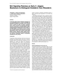
FIGURE 14.1. Viewing multidimensional LSM data. In order to make maximum use of imaging resources, multidimensional CLSM images are routinely
viewed away from the microscope. “Thick” 2D oblique sections (A, B) can be extracted at moderate rates by many software packages. 2D orthogonal sections
(C–E) can be viewed at video rate. Reconstructed 3D views (F, G) require more extensive processing, now common in all commercial systems. (A–D, F, G) are
reflection images of Golgi-stained nerve cells. (E) Multiple xy views (e.g., from an animation) of fluorescently stained nerve cells.
E

284 Chapter 14 • N.S. White
A B
C D
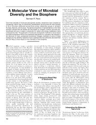
FIGURE 14.2. Identifying unknown structures. It is important to make as few assumptions as possible about the imaged structures during the exploratory
phase of 3D visualization. Average (or summation) projection (A), though simple, often gives low-contrast views due to the low weight given to small structures.
Maximum brightness (B) gives higher weight to small bright structures but when used in isolation provides no z-discrimination. (C) Background thresholding
(setting to zero below a base line) is simple, easy to interpret and increases contrast in the view. (D) Re-orientating the 3D volume (even by a few degrees)
can show details not seen in a “top down view,” and coupled with animation (see text), this is a powerful exploratory visualization tool. (A–C) processed by
simple z-axis projections, (D) “Maximum intensity” using the Lasersharp software. Lucifer Yellow stained nerve cell supplied by S. Roberts, Zoology Department,
Oxford University.
Highlighting Previously Elucidated Structures
Having ascertained the importance of a particular feature, the next
step is to enhance the appearance for presentation and measurement
(Fig. 14.3). Connectivity between voxels in, for example, a filament
or a positively stained volume, may be selectively enhanced
(the extracted structures may even be modeled as graphical tubes
or solid objects; see SoftWorx from API and Imaris packages for
examples). A threshold segmentation band can be interactively set
to remove intensities outside the particular structure. 3D fill routines,
3D gradient, dilation, and other rank filters are the basis for
structural object segmentation. Opacity (reciprocal to transparency)
is possibly the most used visualization parameter to highlight
structures segmented by intensity bands. This parameter
controls the extent to which an object in the foreground obscures
features situated behind it. Consequently, it artificially opposes the
intrinsic transparency of biological specimens. Artificial lighting is
applied during the final stage. Artificial material properties (such
as opacity, reflectivity, shininess, absorption, color, and fluorescence
emission) are all used to simulate real or macroscopic objects
with shadows, surface shading, and hidden features.
Visualization for Multi-Dimensional
Measurements
Often, the final requirement of objective visualization is the ability
to extract quantitative measurements. These can be made on the
original image, using the reconstructed views as aids, or made
directly on the display views. The success of either of these
methods depends on the choice of reconstruction algorithm and the
objective control of the rendering parameters.
Table 14.2 gives an overview of visualization tools that might
be useful for objectively exploring the image data (see also
Chapter 15, this volume).

Visualization Systems for Multi-Dimensional Microscopy Images • Chapter 14 285
A B
C D
FIGURE 14.3. Enhancing and extracting objects. Having elucidated a particular structure within the volume, filtering and segmentation permit selective
enhancement. (A) “Maximum intensity” view [as in Fig. 14.2(B)] after two cycles of alternate high-pass and noise-reduction filters on the original 2D xy sections
(using 3 ¥ 3 high-pass and low pass Gaussian filters). (B) More extreme threshold segmentation to extract the enhanced details during the projection. (C,D)
two rotated and tilted views (Lasersharp software) using a “local average” (see text) to bring some “solidity” to the view. This example shows the principle
danger of segmentation, that of losing fine details excluded from the intensity band.
TABLE 14.2. Overview of Visualization Parameters Desirable for Visualizing Multi-Dimensional Biological
Microscopy Data
Processing step Parameter Minimum required Desirable enhancements
a 3D algorithms General modes Xy, xz, yz orthogonal slices Arbitrary slices, Voxel a-blending
Z-weighted “projections” Surface rendering
Quick modes Fast xy, xz slices Hardware acceleration, Sub-sampling data
Maximum projection
b Controlling the Visualization parameters Projection angles Viewing angle, z-fill, Data threshold,
reconstruction z-stretch Voxels/surfaces, Shading control, Lighting controls,
process Animation controls Material properties, Opacity, SFP/“special” modes,
Sequence (movie) mode Perspective, Batch processing, Post-lighting
Pre-processing tools 2D & 3D image edit n-D image edit, n-D filters, image restoration z-correction,
2D image rank filter morphological filters, math operations
threshold/background contrast
c Interactive controls Visualization parameters Slice positions rotation angles All render parameters, Data/view angles, View
data threshold animation controls Zoom & pan, “Real time” control
Measurements on image 2D measures on slices 3D measures on slices, n-D measurements
Measurements on views 3D measures on views, n-D measurements
Simultaneous measures Multiple measurements on screen Measures auto, Tracked in both displays
on image & views
a The range of 3D algorithms indicates diversity of modes for tackling various kinds of image data, while the quick-look modes include general sectioning and the fastest
voxel algorithms. Simple projections and section movies are always faster than more sophisticated reconstruction modes. b Control of the visualization process suggests the
range of parameters that the user can modify directly to influence the resulting views. More controls give more flexibility but also more complexity in use.
c A very rough idea of the level of interactive control (i.e., rapid changes of the result in response to mouse clicks, etc.) for visualization and for measurements on source
image data and/or reconstructed views. n-D = any number of multiple dimensions.

286 Chapter 14 • N.S. White
WHAT CONFOCAL LASER SCANNING
MICROSCOPY IMAGES CAN THE
VISUALIZATION SYSTEM HANDLE?
Image Data: How Are Image Values Represented
in the Program?
Storing the Image Values
All digital microscopes produce image data values from analogto-digital
(A/D) converters. These will be packed into one or more
8-bit byte values, each of which may have an uncalibrated intensity
range of 0 to 255. Greater collection precision is possible by
integration, averaging, or other high-dynamic-range filtering operations.
However, improvements in electronics and detectors
now make possible the direct acquisition of 12-bit, 16-bit, or even
higher precision digital data. Single-byte storage is more efficient,
and is adequate, for the majority of purposes, particularly for
results from low photon-flux imaging of living cells. It is supported
by all packages. Some instruments allow 16-bit storage (a range
of 0 to 65,535). Intensity data digitized by 12-bit A/D converters
(standard in most current LSMs) is usually packed and unpacked
into 16-bit words by the loss-less conversion:
I16 = I12 ¥ 16 + 15
This slightly cumbersome conversion is necessary to correctly
rescale values in the range 0 to (2 n - 1) without any rounding
errors. The 16- to 12-bit operation is rapidly achieved by bit-shifting
the binary 12-bit values towards the high byte and filling the
additional 4 bits with 1s. This operation can be precisely reversed
for any integer value in the range. Sixteen-bit processing of original
8-bit or 12-bit data may also be desirable for derived images
such as those from some fluorescence ratio experiments. However,
this is excessive for the majority of confocal fluorescence images,
which seldom record more than a few hundred photons/pixel and
therefore have 10% to 20% shot noise (see Chapter 2, this volume).
Microscopy image pixel values and views are economically represented
by integer values. Permanent floating-point storage is
rarely supported. Floating-point calibrations of integer data are
discussed in the following section.
A distinction should be made between storage and display precision.
Historically, some digital microscopy systems have used
the display memory as both a recording and a view buffer with a
built-in image or signal processor. Current approaches use a virtual
display in main computer memory, which is copied to the display
view, allowing decoupling of data and display view and greater
storage precision than video memory if required. This is necessary,
for example, for storing and displaying intermediate results in
image restoration programs.
Image processing systems developed for cross-platform
compatibility (see Amira, Image/volumeJ, and AVS examples of
packages running over four platforms) have always used virtual
displays allowing arbitrary precision images and views to be
manipulated with as little as 5- or 6-bits of display depth per
primary color. The price of this flexibility used to be a significant
reduction in interactive visualization and display speed, caused by
the loss of direct processor access to the video memory. One solution
is to isolate platform-specific accelerations and link them to
core routines when porting to high-performance workstations with
non-standard hardware. Although this approach allows the rapid
introduction of new proprietary hardware, it has now been almost
universally superseded by the use of agreed platform-independent
hardware standards with a defined software interface. Of the
several contenders for a universal graphics standard the clearly
adopted winner is the OpenGL scheme [see http://www.
OpenGL.org and Woo (1999) for details of the OpenGL software
programming interface]. This evolving scheme adds definitions for
the handling of new technologies as they are introduced into each
newly released OpenGL compatible display card or system.
Calibrating the Image Data Values
Multi-dimensional microscopy instruments provide the means
for obtaining accurate and repeatable quantitative measurements.
All parameters including calibration must be linked to the corresponding
image for inclusion in subsequent processing stages. A
discussion of file formats follows the section on image dimensions.
Software packages normally use their own internal calibration
structures because most of the general or so-called standard image
formats do not support all the parameters necessary to fully
describe multi-dimensional microscopy data.
It might be thought desirable to store directly calibrated real
number data values. A fixed-precision mantissa and exponent
would certainly provide consistent relative accuracy, regardless of
the magnitude of the data values. Constant precision could,
however, be maintained by using a logarithmic digitization (or
detector) response. This is consistent with the fact that the presence
of shot noise means that, if gray levels are separated by one standard
deviation they must become wider as the signal level
increases. More bits would then be assigned to low intensities and
less to brighter values. A fixed precision (log) calibration could then
be attached to the 8- or 16-bit integer data values. The minimum
requirement is a floating-point offset (the real value of a 0 pixel),
an increment (the real increment/pixel value), and at least a text
label or key for the linear parameter represented [e.g., log (intensity),
concentration, pH, etc.]. Nonlinear changes require a look-up
table (LUT) for calibrations. Multiple-channel images require separate
calibrations for each component. Ion imaging data need at
least a fixed precision calibration and often a sigmoidal scale
(defined by Rmin, Rmax, and K; e.g., Bolsover et al., 1995). Table 14.3
summarizes data value calibration, arithmetic, and measurement
requirements for a multi-dimensional visualization system.
What Dimensions Can the Images and
Views Have?
Programmable scanning capabilities of all LSM instruments,
motorized focus and/or xy-stage control of any microscope, and
spectral or time-lapse capabilities yield images with a number of
spatial, temporal, and other dimensions. Point-scanning LSM
instruments normally acquire a temporal (sequential) and spatial
(line) scan in the x-axis, repeated at further time points and optionally
at progressive y- and/or z-axis positions. Hence, spatial and
temporal sampling dimensions are simultaneously generated. In
this way, xy, xt, xz, etc., 2D sections and xyz, zyt, xzy, xzt, etc., 3D
volume images are collected. Time-lapsed volumetric (e.g., xyzt,
etc.) or multi-channel spectral (e.g., xyzc, xyct, etc.) are examples
of 4D images. Once considered no more than a curiosity by biologists,
new dimensions of data are becoming routine. The possible
five-dimensional (5D) (x, y, z, t, c) imaging space can now be augmented
with xy- (stage) position (dx, dy, dz), spatial rotation (q, f,
n), lifetime (t), polarization angle (P), polarization anisotropy (r).
This makes 3D to 6D data (from 12 or more possible dimensions
available on a given system) a routine target for data management.
Visualization systems need to support multi-channel images
(Tables 14.3, 14.4, 14.6). Although ultimately, each channel is
processed separately and the results merged together for display,

visualization packages must now manage these parallel operations
seamlessly in order to show multi-channel changes interactively.
This is particularly important where interaction between the values
across channels is required by the chosen algorithm (e.g., the
Imaris SFP algorithm allows transparency in one channel to alter
the simulated light emission from another fluorochrome channel).
Image editing is required to extract (1) subregions of a large
data set or (2) a structure from the complexity of surrounding features.
Sub-region editing should be available through each of the
many possible dimensions of the data. All these dimensions must
be appropriately treated, for example, correctly calibrated, if the
results are to have quantitative validity.
Image Size
Maximum image dimensions should support the full resolution of
the instrument (see Table 14.4). In extreme cases, several adjacent
sections or even volumes may be co-aligned (by correlation and
warping) and tiled together to form a single giant data set (e.g.,
Oldmixon and Carlsson, 1993). Generally, total image size should
be limited only by the available memory. Virtual memory management
provides transparent swapping of programs and data
between RAM and disk. This increases run-time significantly but
can enable very large data sets to be processed. Many software
developers prefer to implement a proprietary mechanism of image
caching or data swapping between RAM and disk, even with the
built-in capabilities of the Windows family of operating systems.
The best way to minimize these overheads is by careful crafting
of the visualization algorithm. The plummeting price of RAM
makes the use of ever more memory irresistible by the programmer,
and thus inevitable by the end user.
Anisotropic Sampling
Most multi-dimensional microscopes are operated with different
sampling steps in two or more axes. Visualization software must
produce views with correctly proportioned dimensions and preferably
have the ability to expand or contract each individually (Table
14.4), for example, artificially expanding the z-dimension of an
image through a thin preparation (such as a biofilm or a stratified
tissue) to highlight the morphology in each layer. The most concise
way of specifying this aspect ratio information is to apply a cor-
Visualization Systems for Multi-Dimensional Microscopy Images • Chapter 14 287
TABLE 14.3. Overview of Image Data Handling Features for Visualizing Multidimensional Biological Microscopy Data
Data handling feature Parameter Minimum required Desirable additional enhancements
a Data storage Types byte Integer, fp, real
Bits 8, 24 (3 ¥ 8) 12/16, 24 (3 ¥ 8), 36/48 (3 ¥ 12/16), n ¥ 8
Channels R,G,B, included, Merge function Arbitrary no. of channels n-channel merge
b Calibration of intensities Linear, Offset, Range Non-linear, Log, Sigmoidal, arbitrary
Intensity measures (distribution 2D Point, 2D Line 3D point, 3D line, trace,
of pixel values) 2D Arbitrary area 3D area (surface),
Summed area volume Arbitrary 3D volume,
2D histogram Results histograms,
ASCII file output DDE to Excel
Math operations +,-,/,* logical, Contrast/gamma mapping, Trig functions, Log
Manual z-weighting Auto z-weighting
a All systems support 8-bit (byte) data types. A few allow higher precision. This is useful for high dynamic range images. The use of 8-bit indexed or 16-bit “hi-color”
modes for multi-channel data is now less common than 24-bit RGB support. Most scientific CCD cameras and LSMs now support 12-bit data (usually packed into 16-bit
words) but few packages support these data types for visualization.
b It is important to clearly distinguish calibration of the intensity data values from the image dimensions (Table 14.4). Calibrated intensities also allow real values of pH,
Ca 2+ , etc. and other concentrations to be visualized.
rection factor to the appropriate axis calibration. This should be
done interactively so that some imaging distortions can be corrected
(e.g., for a specimen such as skin with layers of different
refractive index). This does not change the data values in any way
and is preferable to resampling the entire data volume, which
would tend to use up precious memory. When the data is subsequently
processed or displayed, a floating-point z-stretch parameter
(and equivalents for x, y, etc.) would correctly specify the
spacing of each plane. An integer z-fill parameter represents the
number of equally spaced sections to optionally add between each
of the repositioned planes. These extra data values are derived by
interpolation, by pixel replication or linear, cubic, or higher polynomial
spline. An obvious question arises here: How real are the
extra data points? A priori knowledge of the specimen and imaging
system is required for an informed choice. On-the-fly data expansion
during processing will conserve storage space but requires
more computations. Pre-expansion, for example, during the image
loading cycle, will optimize processing speed at the expense of
memory. A good compromise is rapid expansion during the computation
using precalculated linear geometric LUTs.
Calibrating the Image Space
To make measurements, image and view dimensions must have the
correct calibrations (Table 14.4). These must be updated during
any resampling, zooming, and image editing. Minimum requirements
for each dimension are again floating-point values for offset
and increment, and an axis label. Warping conveniently handles
nonlinear dimensions by resampling onto a rectilinear grid. Correction
of acquisition errors should ideally be incorporated into a
single intensity and sampling interpolation. These errors include:
• Spherical aberration caused by mismatch between the refractive
index of the immersion medium, the imbibing medium and
the design of the objective.
• Axial chromatic aberration (a focus shift seen with all
objectives).
• Lateral effects, such as chromatic magnification error.
• Photometric signal attenuation and correction of geometric
distortions from refraction within the sample (e.g., Carlsson,
1991; Visser et al., 1991, 1992; Fricker and White, 1992; Hell
et al., 1993) are desirable preprocessing tools.

288 Chapter 14 • N.S. White
TABLE 14.4. Overview of Desirable Image and View Dimension Parameters for Visualizing Multi-Dimensional Biological
Microscopy Data
Feature Parameter Minimum required Desirable additional enhancements
a Image dimensions Single plane Full un-edited image (from camera, Unlimited
LSM etc), Held in RAM Display independent
Multiple images in RAM
Total image size Fully sampled 3D image, Unlimited, Display independent, Multiple 3D images in RAM,
3D image in RAM n-D images in RAM, efficient caching
b Supported dimensions 2D, 3D n-D, View angles, Rotation angles, Stage position, Polarization/
x,y,z time anisotropy, Lifetime
Editing the dimensions Sub regions (ROI) 2D sub-area, 3D sub-volume, edit 3D arbitrary sub volume, Edit in view, 3D cut-away, n-D ROI
(geometric operations) on slices
c Data corrections Background normalization Non-linear corrections, Photobleaching, Flat field, n-D
z-atttenuation corrections, Optical corrections, Image restoration
Z-geometry z-stretch Integer value Real value
linear Non-linear (e.g., cubic, etc.)
z-fill Integer for large angles Adaptive for chosen angles
View dimensions Single view 3D diagonal of image Unlimited, Display independent
View movie in RAM Multiple views in RAM
JPEG compression Efficient caching, Efficient compression
Number of views 120 views (360 ¥ 3degs) Unlimited, Display independent
Multiple movies in RAM
Channels in view R.G.B Arbitrary no. of channels
d Calibration of Image X,y,z,t All dimensions
dimensions View X,y,z,t,angle All dimensions
Dimension measures On image 2D Point, 2D Line, 2D histogram, 3D point, 3D line, trace,
2D Arbitrary area, ASCII file output, 3D area (surface), Arbitrary 3D volume,
Summed area volume, Results histograms, DDE to Excel
On view 3D point, 3D line, Trace, 3D area (surface), Arbitrary 3D volume,
Results histograms DDE to Excel
a In most cases the image data space is limited only by the amount of disk and/or memory available. The operating system and/or the application program may provide
virtual memory management and disk caching.
b Most packages can handle time, spectral, etc., data as for a “z-stack” but few can directly interpret time or wavelength calibrations with any meaning.
c Complex corrections usually involve sample-specific data and some pre-processing.
d Calibration of dimensions should be clearly distinguished from those of the data intensity values (Table 14.3).
n-D = any number of multiple dimensions.
Standard File Formats for Calibration
and Interpretation
While there are many standard formats, there is no universal
standard currently adopted for microscope images. However,
there are established imaging formats (e.g., DICOM, see
http://medical.nema.org/) that are routinely used by visualization
packages such as the Cedara, Vital Images, and Analyze software
that fully describe multi-dimensional volume data from medical
scanners. As LSM and other research microscopes become more
routinely used as screening instruments and for clinical applications,
it is hoped that such standards will become routine from
these suppliers as well. A catch-all image input facility such as the
RAW options offered by many programs allows any packed binary
file with a fixed-size header to be read in. Microscope instrument
manufacturers have taken one of two options: (1) developed a
completely proprietary structure and made this available to other
developers and users, or (2) taken an existing extendable format
(such as the Tagged Image File Format [or TIFF]) and added
system-specific components (e.g., for TIFF, licensed specific tags)
to store the extra acquisition parameters. A problem with this
second approach is the necessary proliferation of a number of variants
or compliance classes of such formats. Any third-party reader
program must recognize (and provide updates for) several different
versions. A widely adopted alternative is to use a proprietary
structure and to provide conversion tools to import/export data via
standard formats. Unsupported parameters are transferred into the
program by an ad hoc semi-manual process.
A flexible, industry-standard approach to image-related details
is to use a conventional database to store preprogrammed fields of
information (sometimes a third-party software product is used with
the visualization tool — such as the ImageAccess database used
by Imaris — which can manage all image and image-related files).
Two types of information must be stored and linked with each
image: (1) instrument-specific details describing the instrument
settings used for the collection and (2) image-specific information
describing the dimensions, calibration, and experimental details.
The database can hold both sets of details, together with a pointer
to the image data (or even the image data itself for small images).
Alternatively, the database may hold just the system configurations
used as stored settings or methods (e.g., the Bio-Rad Lasersharp
program stores all the instrument and user settings in a Microsoft
Access database). This latter approach requires a pointer to the relevant
settings to be saved with the image data, separately from the
database. Table 14.5 summarizes some important image and view
data parameters.
Processing Image Data
Less obvious than the storage representation are the data type and
precision used during computations. Floating-point representations

educe rounding errors during geometric transformation interpolations.
Even this requirement for floating-point representation can
be partly avoided by either (1) combining several interpolation
steps into a single, composite geometric and photometric transformation,
or (2) increasing the sampling by a factor of at least 2
for each subsequent interpolation. This second approach is somewhat
extravagant in terms of storage and will not help if the sampling
is already at the Nyquist limit. The processor architecture is
an important factor in determining the processing speed. Fast
multi-word and floating point arithmetic is now standard in microprocessors.
Despite this, some instruments, notably the Zeiss range
of LSMs, use specialized, programmable digital signal processors.
Processor Performance: How Fast Will My
Computer Process Images?
Personal computer (PC) performance for image manipulation is
constantly improving, making the specification of system performance
in a text such as this somewhat pointless. However, the
principal components of the computer system required can be
described in terms of their relative importance to performance.
At the time of writing, the Pentium PC processors are the
norm, running at around 4GHz with bus speeds around 1GHz.
These are very approximately 30 times faster than 10 years ago,
representing a doubling of speed every 2 years. Non-Intel processors
with alternative combinations of price/performance through
low power consumption, higher capacity of on-chip memory for
data caching, and other enhancements appear from time to time
with advantages in different applications. Alternative Intel processors,
such as the Xeon, also compete in these areas and offer
improved workstation and multi-processor performance. Provided
the software is correctly designed, transfer bottlenecks can be
reduced with a processor having at least 512kB of level 2 memory
cache. Apple Macintosh machines have undergone something of a
renaissance in recent years; the current G5 is broadly equivalent
to the latest Pentium devices, and still have competitive and equivalent
components for efficient numerical performance and a highly
optimized bus for image transfers. The current Macintosh OS X
Visualization Systems for Multi-Dimensional Microscopy Images • Chapter 14 289
TABLE 14.5. Overview of Desirable File Format and Image Information Features for Visualizing Multi-Dimensional
Biological Microscopy Data
Feature Parameter Minimum required Desirable additional enhancements
a Image file format Proprietary standard Fully defined open source Fully defined open source, Full range of conversions,
Multi-file TIFF, AVI (for series) A Universal standard!
View file format Proprietary standard Fully defined open source Fully defined open source, Full range of conversions,
Multi-file TIFF/BMP, JPEG, AVI Efficient compression, A Universal standard!
b General params. stored Size All dimensions All dimensions
Calibration X,y,z,t dimensions All dimensions
Annotation ROIs ROIs, Text, pointers
Microscope Data specific parameters All instrument parameters, Experimental parameters,
Stored in image format, or ASCII file Stored in image format and/or database
Notes User/exp notes, Informatics
Special view parameters Source image Image filename, Links in database etc., Visualization
stored history/log
Orientation etc. Rotation angles, etc.
Visualization parameters Algorithm name, Algorithm parameters, Display options
a Proprietory file formats are used by most systems. “Standard formats” such as TIFF may also cause confusion as there are many different compliance classes of TIFF, so
only a sub-set of the TIFF tags in a particular file may be recognized by a given reader.
b Some parameters may be stored with the image data in the same file, in a separate (e.g., ASCII) file or in a database. It is important to know the whereabouts of this information
if the image is to be taken to another program with the associated data intact. ROI = region of interest.
operating systems have been significantly updated and based on
Unix technology in order to take advantage of the large software
developer base. Unix workstations are still a costly alternative to
ever-improving PC platforms. Improving processor performance
alone is still reflected in the voxel rendering performance (in
voxels/second or vps) for visualization of multi-dimensional
microscopy data.
Improvements in other areas of the PC have been either
necessary to keep pace with the processor speeds or provided
enhanced capabilities directly. Hard disk drive data transfer speed
can limit the speed of animations (movies) and 3D visualization
when applied to large data sets. At the time of writing, so-called
ultra-fast, ultra-wide SCSI interfaced devices, with capacities up
to 250Gb per disk still have higher performance than IDE devices
and tend to be more robust and easier to upgrade, although plugand-play
technology makes this last issue less important in the
latest PCs. The latest PCs and Macintosh computers can access
4 to 8Gb of RAM. This is adequate for most multi-dimensional
data sets but will inevitably still limit performance if many large
data sets are opened simultaneously, especially if the software is
designed to read in the entire data set and/or the system caching
or swap file is inefficiently configured for the ratio of disk to RAM.
Computer video display subsystems have, over the last 10
years or so, taken on more and more graphics processing operations,
allowing greater optimization and relinquishing the general
purpose CPU for other tasks. The display system has become a
dedicated graphics processing unit (GPU) and up to 256Mb of
dedicated display memory. Some entry-level PCs may still use portions
of main memory, set aside for access by the display, but these
are not recommended for multi-dimensional visualization. Many
functions are carried out by dedicated hardware and/or firmware
running on the GPU and associated devices. Depending on the
sophistication of the chosen graphics system, supported operations
may include:
• Rapid display of 2D views for animations, etc.
• Rendering of surfaces composed of triangle or other polygon
primitives.

290 Chapter 14 • N.S. White
1.E+06
1.E+05
1.E+04
1.E+03
VPS/MHz
VPS/1000
Voxel Rendering Speed
SGI SGI SGI Pentium Pentium Pentium Pentium Special
R4400 R4400 R4400 PC PC PC PC hardware
(150MHz) (150MHz) (150MHz) (200MHz) (200MHz) (200MHz) (1.5GHz)
FIGURE 14.4. Voxel rendering speed: dependence on hardware performance.
When assessing a visualization system, many factors need to be taken
into account (see text). Parameters for individual performance figures should
be assessed with care. On standard platforms, processor speed is still an important
factor. From a simple ratio of voxels processed per second per MHz processor
speed (with a basic algorithm) a figure of merit can be obtained. Running
the same a-blended. voxel-rendering software (Voxblast) on multiple Pentium
processors gives broadly the same figure of merit as single processors
when normalized for the total processor speed. The same is found for multiprocessor
graphics workstations. Running on special hardware (this example
is the VolumePro board) sacrifices portability across platforms but (as has historically
always been the case) gives vastly improved performance.
• Geometric manipulations (e.g., warping of data vectors).
• Rendering of voxel objects.
• Transparency/opacity of graphics and voxel objects.
• Artificial lighting and shading.
• Rapid manipulation of color or grayscale.
• Panning and zooming of the display.
• Texture mapping (used to rapidly render image layers onto a
growing display view).
Figure 14.4 shows some approximate voxel rendering speeds
that might be expected over a range of processing platforms (data
corresponds to rendering speeds of Voxblast from Vaytek Inc.).
Optimization of the GPU functions is controlled largely by the supplied
driver software and contributes to the major differences
between various hardware configurations. CPU operations are
coded by the application programmer and this is also reflected in
the performance of the software. The relative efficiency of these
two aspects can have an important influence on the effectiveness
of the package as a whole. An effective visualization algorithm for
multi-dimensional data must include optimized numerical loops
(particularly nested sequences) and use fast indexing into preprocessed
parameter LUTs for frequently used values. The following
section describes some of the optimizations that are
responsible for the performance range seen between different
programs.
HOW WILL THE SYSTEM GENERATE THE
RECONSTRUCTED VIEWS?
Assessing the Four Basic Steps in the Generation
of Reconstructed Views
(1) The image (or a subregion) is loaded into the data space
(an area of computer memory). Preliminary image editing, preprocessing,
and/or analysis is used to define calibrated image values
with known dimensions. This constitutes the input to the visualization
process. Packages such as Analyze have some useful preprocessing
capabilities (Robb, 1990). Alternatively, a more general
program such as Metamorph, ImageJ, and Image Pro, etc., can be
run alongside the visualization package for image preprocessing
(or the visualization component can be added to the 2D package).
(2) A view must be chosen (subject to the available reconstruction
algorithms) that will produce the most flexible and appropriate
representation of the image data. An intelligent choice of
view can minimize the number of reprocessing cycles (see also He
et al., 1996; Marks, 1997; Kindlmann and Durkin, 1998, for
attempts at computer-assisted choice of visualization algorithm).
The visualization step consists of two transformations: First, a geometric
orientational mapping of the image space into the reduced
dimensions of the view, and, second, a photometric mapping
(sometimes called a transfer function) whereby the image intensities
are processed to determine the brightness of a pixel at each
position within that view.
(3) The display step consists of a second geometric and
photometric mapping that together constitute output or matching
of the multi-dimensional view into the available physical display.
In practice this may consist of scaling and copying or a more
complex operation (e.g., animation or stereoscopic presentation).
These presentation or output options, dictated by the display space
capabilities, will determine the most efficient use of screen resolution,
color, animation, etc. In turn, these will influence the choice
of appropriate reconstruction algorithm.
(4) Dimensional loss during the visualization processing is
partly restored by the display step and partly by a priori knowledge
used to interpret the 2D display view (e.g., depth cues, animation,
stereo, etc.). Inspection and analysis of the display view
is the last step of the visualization process.
The next sections describe more details of these processes that
are important for microscopy images using techniques found in the
systems listed in Table 14.1.
Loading the Image Subregion
Any image processing program must first open the image file, read
and interpret the file format information, and then load some or all
of the data values. Interpretation of the file format largely determines
the flexibility of subsequent manipulations. An on-screen
view of (1) image sizes (in pixels and calibrated units), (2) intensity
data calibrations, (3) associated notes and (4) a quick-look
reconstruction will aid selecting the required image or subregion
(Analyze and Imaris, e.g., show image volumes as thumbnail pictures
with a grid showing the image dimensions, etc.). The file
format information will determine whether the data needs resampling
to produce correct image proportions, and interactive
adjustment is essential for z-stretch/fill (see above). Interactive
photometric rescaling or segmentation (in combination with a
simple volume representation) are essential to remove (e.g., set to
zero or ignore) background values that would unnecessarily

slow down computations. Multiple passes through the data will
be time consuming for large images. A single composite geometric
and photometric resampling (using fast LUTs) should be combined
with loading the data from disk. Data expansion options
(e.g., z-fill) may be temporarily restricted to speed up computations
during the exploratory stages. Flexibility and control at this
stage must be balanced against the efficiency of a single processing
stage. Some image preparation options are detailed in
Table 14.2.
Choosing a View: The 5D Image Display Space
As introduced above, the efficient use of all the available display
space greatly increases the flexibility of visualization algorithms.
The 2D Pixel Display Space
Pixel resolution must accommodate a reconstructed view at least
as big as the longest diagonal through the 3D volume. This means
that, for example, to reconstruct a 768 ¥ 512 ¥ 16 frame 3D image
with z-stretch of 4 and arbitrary rotation, the display view that will
be generated in memory could be up to 950 pixels square. For the
same computation and display of 1024 ¥ 1024 pixel frames, 1450
pixels square are required to avoid clipping. As it is advisable to
display the views without resampling, these values represent the
minimum display window in pixels. Processing time may dictate
that only a subregion can be processed but, in general, display of
a single full resolution frame should be considered a minimum.
Although the display pixel range may be only 8 bits/channel, the
ability to generate projected views with a higher intensity range
(perhaps 16 bits) means that, for example, average projections of
images with dimensions greater that 256 pixels can be made with
no loss of detail. It is now standard practice to produce an output
view that is independently rescaled according to the size of the
display window as defined by the user. This is transparently
handled by the software and display driver. However, rescaling can
always give rise to unwanted aliasing effects so it is wise to restrict
the display zoom to integral multiples of whole pixels. The application
program, perhaps using features of the display driver, may
allow an image of greater size than the physical display to be
rapidly panned, giving access to display views of almost unlimited
size. High-resolution non-interlaced displays are now standard for
all computers. Although a single display may deliver resolutions
up to 2650 pixels, it is now standard practice to provide multiple
screen outputs from the best display systems. In this way, desktops
of perhaps 2560 ¥ 1024, 3200 ¥ 1200 or more can be spread
seamlessly across a pair of similar monitors placed together. The
display drivers will automatically handle traversing of the mouse
and program windows between the physical screens or even allow
large images to straddle the entire display space. (A commonly
recommended supplier of multi-view compatible OpenGL graphics
cards for PCs is nVidia, http://www.nvia.com, while on
Macintosh’s they are built in.)
The Color Display Space
Color is a valuable resource for coding multi-dimensional information
on a 2D device. It is important to ascertain the number of
different colors that can be simultaneously displayed, as distinct
from the number of possible colors present in the data or display
view. The author prefers the generic term palette to represent the
subset of simultaneously displayable colors and color resolution
to indicate the full set of possible colors present in the data.
Although many different graphics display resolutions have been
used by imaging systems in the past, the plummeting cost of hard-
Visualization Systems for Multi-Dimensional Microscopy Images • Chapter 14 291
ware have made the use of all 8-bit displays redundant. Useful
display systems will be encountered that have either 16, 24, or 32
bits per pixel of display depth. It should be carefully noted that a
display system may have additional memory associated with each
pixel for storing other values important for controlling the display
process, but here we are concerned only with the color and intensity
information. A standard 24-bit display has 8 bits of memory
storing 1 of 256 possible values each of red, green, and blue intensity.
Additional display panes are available in 32 bit modes. With
2 24 possible display colors (over 16 million), a 4000 ¥ 4000 pixel
image could display each pixel with a different and unique color.
There is, therefore, significantly more contrast available in a color
image than in a monochrome (e.g., grayscale) representation.
However, it must always be remembered that the actual red, green,
and blue colors corresponding to each component are fixed by the
spectral characteristics of the physical screen material. These will,
in general, never coincide with filter spectra of the microscope, or
even with the nominal red, green, and blue characteristics of a
color camera.
When more than 24 bits of data are stored for each pixel of the
display view, such as for a 3-channel 16-bit color image (a 48-bit
data set), the visualization software must resample this down
to the available color space of the display system. An extreme
example is the option in the Imaris program of having color-space
computations carried out with 96-bit precision as opposed to 24bit
precision, improving accuracy at a 4-fold cost in extra memory.
However, at present cathode-ray tube (CRT) and liquid-crystal displays
(LCD) are capable of displaying little more than 8 or 9 bits
of data in each color channel.
Pseudo Color
Pseudo or indexed color was used by older 8-bit displays. It is now
only really important when a display system of very high resolution
is implemented, for cost purposes, with 16 bits of high color
pixel depth. Each of 65,536 entries (for a 16-bit mode) or 256
entries (for 8-bit modes) in a color look-up table (CO-LUT) is
assigned a unique composite RGB value. This CO-LUT is an
indexed palette and can be rapidly updated or modified to change
the displayed colors without altering the view data values. It is the
CO-LUT value pointed to by each data value that determines what
RGB intensities appear on the monitor. Visual perception of color
is far more acute than for intensity in bright VDU displays because
cone density in the eye is highest in the fovea (Perry and Cowey,
1985). Pseudo color is, therefore, useful for presentation of
calibrated 16-bit maps of image intensities, for example, from ion
indicators. In general, it adds contrast to subtle changes in (1)
brightness, (2) temporal, or (3) coordinate (typically z-relief)
views.
True Color
True color means any display element can have independent values
for each of its red, green, and blue components. The simplest
way of representing these in a byte-structured format is a 24-bit
(3 ¥ 8 bit) RGB voxel. Other color-coding schemes are possible.
Hue, saturation, and brightness (HSB) are useful for intensityindependent
color transformations. Process color space (using
cyan, magenta, yellow and black — CMYK) is the form used for
hard copy and publication. RGB values map directly into a 24-bit
display with no intermediate processing. Color manipulations can
be carried out by modifying the component color data directly.
Alternatively, each 8-bit channel may be driven by a monochrome
(R, G, or B) 8-bit indexed CO-LUT (palette).

292 Chapter 14 • N.S. White
Multiple-Channel Color Display
Either color or brightness resolution (or both) can be traded for
extra channels. A hue (preferably non-primary, i.e., magenta, cyan,
yellow, orange, etc.) is defined by a unique RGB ratio for each
channel. An intensity (brightness) scale in each hue then represents
the indexed data values of that channel. All channels are combined
into one true-color RGB view, adjusted to fit the display resolution,
that is, each channel using a segment of the available palette.
Figure 14.5 includes examples of the use of color for 3D multichannel
and stereo display.
Animations
As with pixels and color, the temporal display space can also be
effectively used for visualization. The simplest temporal mapping
is the sequential display of view sequences. Temporal range is
determined by the number of frames that can be stored for rapid
animation. Time resolution has two components: the frame rate
(the time between successive views) and the refresh rate (how fast
a single view is updated) (Table 14.6). The refresh rate contributes
significantly to the perception of smooth animation. Retinal persistence
results in a screen refresh rate of £1/18th of a second
being perceived as virtually instantaneous. For through-focus
sequences, fading between frames is advantageous. A long-persistence
display phosphor (such as on older video-rate monitors)
assists this fading process for low framing rates £4Hz but contributes
degrading blur at higher speeds. Perception of smooth
motion requires high lateral resolution and visual acuity. Therefore,
smooth rotation animations require (1) fine rotation steps, (2)
a short persistence/high refresh rate display, and (3) an animation
frame rate of above 10Hz (with £0.05s data refresh). Hardware
and software compression/expansion (see Chapter 48, this volume)
are built into some display systems, allowing suitable data to be
animated at up to video rate with reduced storage requirements.
Both RAM-based and hard-disk–based systems can now easily
provide full-color video-rate animation. Screen update is improved
by a double-buffered display comprised of both a visible and a
FIGURE 14.5. Efficient use of the 5D display
space. The upper four images are two “maximum
intensity” stereo-pairs (Lasersharp software).
They were generated with ~8deg of “rotation”
around the y (vertical axis) giving binocular
stereoscopy through the x display dimension and
similar “tilts” around x to give motion parallax
and temporal interpolation depth cues using the y
display axis. In these static views, the top pair tilt
forwards and the lower pair tilt backwards. With
few exceptions, the most efficient use of the color
space is for the display of multi-channel views.
Data (courtesy of Bio-Rad Microscience) is from
a large confocal series from lung tissue. (A)
shows a triple-stained fluorescently labelled pancreatic
islet, with each channel “maximum projected”
and combined into a 24-bit Windows
bit-map view (data collected by T.J. Brelje,
University of Minnesota, Minneapolis, MN). (B)
shows a dividing shrimp embryo stained with
rhodamine-conjugated beta-tubulin antibody (27
five-micron optical sections) rendered using
VoxelView/Ultra. Cell bodies and membranes
(blue) are assigned low opacity so that microtubule
structures (orange-red) can be viewed
distinctly in their cellular context. Analytical
geometric data (lines and surfaces) can also be
inserted, not overlaid, using the VoxelView/Ultra
Embedded Geometry tool. Embedded lines highlight
the axes of division and centers of polarity
of the dividing cells and help indicate directions
of movement during mitosis. (Data courtesy of
Dr. W. Clark, Jr., University of California,
Bodega Marine Laboratory, CA). Intensity gray
levels can also code for z-depth (see text). (C)
shows a Lasersharp “height” view of a living
fibroblast imaged by fluorescence optical sectioning
of an excluded FITC-dextran-containing
medium (see Shotton and White, 1989). (D)
Binary (single-bit) line graphics make inefficient
use of display space. However, this “YMOD” or
height profile of BCECF-stained living chondrocytes
from pig articular cartilage (data by R.J.
Errington, Physiology Dept., Oxford University)
does show relief more clearly than would an
intensity view alone.

second (non-displayed) buffer. The second buffer is updated while
the first is read out to the monitor and pointers to the two buffers
are switched between successive frames. New graphics standards,
especially OpenGL, now fully support double buffering on standard
displays. Double buffering obviously needs twice the memory
on the display card.
Stereoscopic Display
Depth perception by stereo parallax provides a third spatial display
dimension. Some of the geometric z-information can be mapped
into this stereo space. Like the color/intensity range compromise,
the stereoscopic depth requires some reduction in bandwidth of
another component. The two halves of a stereo-pair can be displayed
using screen space components normally reserved for (1)
2D pixel area, (2) color, or (3) sequences (temporal space). Each
of these methods requires an appropriate viewing aid to ensure that
each view is presented only to the appropriate eye. The detailed
implementation of stereo presentations are described in a later
section. Table 14.6 shows some image and view display options
for visualization systems.
Optimal Use of the 5D Display Space
Several conflicting factors must be balanced: (1) visual acuity
in a particular display dimension, (2) efficient use of display
resources, and (3) minimizing processing time. Because intensity
variations are difficult to interpret in a low-contrast image, it is
sometimes tempting to use y-mod geometric plots and other
display tricks to represent, for example, a fluorescence ion concentration.
Using the geometric space rather inefficiently in this
way for a simple intensity display may allow us to view inherently
planar information with greater accuracy. A contrasting example
might be when a depth profile surface can be defined from a 3D
Visualization Systems for Multi-Dimensional Microscopy Images • Chapter 14 293
TABLE 14.6. Overview of Image and View Display Options Desirable Visualizing Multi-Dimensional
Biological Microscopy Data
Feature Parameter Minimum Required Desirable additional enhancements
a Display 2D To show full image 1:1 without clipping As large as possible, Multiple-screens, Seamless desktop
pixel size (typically needs 1280 ¥ 1024 or more)
Color Display mode 24-bit RGB 24-bit of higher + overlays
b Multiple-channels Standard RGB Arbitrary number of channels
Screen Display refresh (Hz) 70Hz ~100Hz
c Size (diagonal inches) CRT: 19 CRT: multi 21, Flat: multi 19, Wide-aspect & Specialist
Flat: 17 Mega-pixel screens
Movie d FPS (Hz) ~10 at full image resolution Up to about 30fps, Motion compression, Variable fps
Variable fps
Recording Store movies as digital file Digital video store, Digital Compression, DVD recorder,
DVD RAM
Hardware assisted z-buffer video system, Compression AV quality disk
system
Stereoscopic Modes Manual stereo pairs Side-by-side, LCD viewers,
Movie pairs Shuttered screen, Projection,
Anaglyph display Non-viewers (e.g., lenticular)
Standard hardware (e.g., OpenGL)
Animation 2 color anaglyph Full color
Auto stereo from 6deg sequence
a Most operating systems and application programs decouple the image size from the display size. If the image must be sub-sampled by the system to display in the chosen
window, aliasing may occur (some graphics systems have anti-aliasing devices built in). Usually, not all of the screen area is available for the image, so the screen needs
to be bigger than the largest image. Some graphics systems allow an image larger than the screen to be “displayed” and the visible part is panned around with the mouse.
b With color-space mixing, it is possible to “merge” an arbitrary number of channels into a standard 3-color, RGB display.
c CRT sizes are usually given as the tube diagonal, not the visible screen size, flat panel displays indicate the actual viewing area.
d The animation software must be highly optimized to deliver the fastest, smoothest framing rates. This can be achieved in software at the expense of standardization and
so the fastest systems may only work with a limited range of display hardware.
FPS = frames per second. LCD = liquid crystal display.
object: (1) the geometric space in x, y, and z (e.g., stereo) could be
used to show the object’s surface relief, (2) color used for material
properties (fluorescence, reflectivity, etc.), and (3) intensity
(grayscale) employed to reinforce z-cues by depth weighting.
Automontage is an interesting application (from Syncroscopy,
Ltd.) where surfaces are extracted by ray-casting projections of
widefield z-focus series. The resultant 3D data is then visualized
using z-profile plots or stereoscopic views.
The best display space for a particular component will depend
on the available resolution and the range of the data. In general,
multi-channel images are best shown as different colors, in which
case depth information must be coded using stereo or motion parallax
or some lighting/shading mechanism. Binocular stereoscopy
works for views rotated around the y-(vertical) axis when looking
at the screen, that is, with parallax shifts in the horizontal x-direction
(Frisby and Pollard, 1991; Poggio and Poggio, 1984) (for an
upright observer!), while motion parallax is perceivable around
any axis within the xy-plane. The perception of depth by so-called
motion parallax is actually a subconscious interpolation of the
images between each view to fill in the path of features presented
at discrete loci along a simple trajectory (Nakayama, 1985; Fahle
and de Luca, 1994). Therefore, a sequence of side-by-side stereopairs
at increasing tilt angles only will give stereo depth in x and
animation depth in y with minimum processing. Rotations are
interpreted more readily by most observers than other temporal
sequences, such as through focus z-series, largely because of our
acute perception of parallax. Detailed assessment of particular presentation
modes requires an in-depth knowledge of the physics and
physiology of visual perception (e.g., Braddick and Sleigh, 1983;
Murch, 1984; Landy and Movshom, 1991). Alternative temporal
coding strategies, such as color-coded tixels (Kriete and Pepping,
1992) thus aid the presentation of non-rotated time series, partic-

294 Chapter 14 • N.S. White
ularly if interactive measurements are to be made. Figure 14.5
shows examples of the efficient use of display space for multidimensional
display.
Mapping the Image Space into the
Display Space
Having chosen both the image dimensions and display space, a
suitable mapping of image space to the output view dimensions
must be found. Choices for this geometry processing are intimately
linked to the implementation of the transfer algorithm for combining
the data intensities, however, it is more useful to consider
these components separately in order to make the most of available
resources; geometry and intensity processing software and
hardware may reside in different subsystems of the visualization
workstation.
For a general multi-dimensional image I(xi, yi, zi, ti, ci, . . .) and
view V(xv, yv, zv, tv, cv, . . .) we can define an overall reconstruction
function (R) such that
V(x v, yv, zv, tv, cv . . .) = R [I(xi, yi, zi, ti, ci, ...)] (1)
where x, y, z are the spatial coordinates, t is time, c is color channels,
etc.
R has two components: a geometric transform (G) converting
image to view dimensions and a compositing (sometimes called
transfer function) or projection operation (P) performed on intensities
through the view space (Fig. 14.6). These components of R
are thus related by
V = P(x v, yv, zv, tv, cv, ...)
where xv = Gx(xi, yi, zi, ti, ci, . . .), yv = Gy(xi, . . .) etc. (2)
The following sections describe various G functions used in visualization
systems (listed in Table 14.7). Projections are described
later (and listed in Table 14.8).
c i
t i
zi yi xi A Multi-Dimensional Image I(x i,y i,z i,t i,c i)
e.g., 3-D
rotate, shift,
reflect, coord
re-map
etc.
G(i)
t v
c v
zv yv xv B Multi-Dimensional View V(x v,y v,z v,t v,c v)
t v
C Sequence of 2D pseudo-color or
RGB display views V(x v,y v,t v)
P(v)
Project objects along the
view axis (e.g., z v) into 2-D
views
Simple Visualization: Reducing the
Geometric Dimensions
This involves discarding all but two of the voxel coordinates
and mapping the remaining dimensions to screen xy-positions. A
non-rotated orthoscopic (non-perspective) view of a 3D (xi, yi, zi)
volume (viewed along the zv-axis) is a simple geometric mapping
of serial sections that can be projected (e.g., by summing,
maximum intensity, etc.) onto a 2D orthogonal (xy)v display (Fig.
14.6). The G function is defined by
x v = xi, yv = yi, zv = zi, i.e., V(xv, yv) = P(xi, yi, zi) (3)
For a 3D time series (x i, yi, ti) to be viewed edge-on, (xi, ti), the
transformation is equally simple:
x v = xi, yv = ti, zv = yii.e. V(xv, yv) = P(xi, ti, yi) (4)
These are the basis of the familiar three-pane orthogonal section
views found in many visualization programs.
Rotations
A single, orthoscopic, x-axis rotation (q) requires a geometric
mapping given by
x v = xi, yv = yicosq +zisinq, zv =-yisinq +zicosq (5)
then V(xv, yv) = P(xv, yv, zv)
The projection is then performed in the (re-oriented) view
coordinates. Offset coordinates (i.e., x i - xo, etc.) are used for rotations
around a point (xo, yo, zo) other than the image center. Rotations
are non-commutative, that is, the order of x-, y-, and z-axes
matters. The observer’s coordinate system (xv, yv, zv) is static, and
all orientations are given in this frame of reference. To generate a
view of the image rotated simultaneously about the three image
axes (i.e., a tumbling algorithm), three consecutive transformations
are required. The first [e.g., a tilt around xi, Eq. (5)] is obviously
y v
x v
FIGURE 14.6. The visualization process. Voxel and object
visualization algorithms proceed in three clear steps: (1)
Multi-dimensional image space (A) is transformed by a geometric
function (G) to the (re-orientated) view space (B). (2)
Selected objects in the view space are combined using a projection
operation (P) to produce a sequence of 2D views. (3)
The 2D views are presented on the display device (C).

Visualization Systems for Multi-Dimensional Microscopy Images • Chapter 14 295
TABLE 14.7. Overview of Image-to-View Space (Geometric) Transformations for Visualizing Multi-Dimensional Biological
Microscopy Data
Feature Parameter Minimum required Desirable additional enhancements
a 2D sections Orthogonal Arbitrary orientation, Section rotation,
Sections with translation Thick sections >1 pixel, Curved “surface” extraction
Projection geometries b Isometric Arbitrary orientation, Full matrix rotation,
Pixel shift (limited angles) Pan & zoom, Combinations (e.g., “fly-by”),
Rotation or tilt With cut-aways
Z-coding “Focus” animation Simple z-movie Interactive arbitrary section movie
On-the-fly section movie
Motion parallax Simple pre-calculated movie Interactive pre-calculated movie, Motion compression,
On-the-fly movie (with interaction)
Stereo parallax Manual stereo pairs Automatic stereo, Stereo with perspective
“Height” views Maximum int z-coordinate Threshold z-coordinate, z-coordinate of high gradient
Perspective Orthoscopic b z-perspective
Time-coding t-movie t-coordinate
l-coding l-movie l-coordinate, Arbitrary color channels
3color channels
Special geometry OpenGL with enhancement, z-buffer hardware “geometry
hardware engine”
a XY orthogonal sections are the basis of “thru-focus animations.” Many systems now permit arbitrary (including “oblique”) sections to be extracted from a 3D volume
quickly enough to be considered interactive. Curved sections (rarely supported) are particularly useful for cellular structures. They can sometimes by produced by preprocessing
using line-segments extracted serially from a 3D stack.
b Isometric and z-perspective mapping (G) functions increase the perception of depth in static views, and remove the ambiguity of depth seen in some rotating projections.
also around xv. The following two transforms (around yi and zi) are
then around oblique (i.e., general) axes in the view space. Our rotation
is thus three separate twists around axes: xi = (ax, bx, cx), followed
by yi = (ay, by, cy) and then zi = (az, bz, cz). The G function,
Eq. (2), for each twist is a formidable computation with three subcomponents
xtwist = x[a 2 + C(1 - a 2 )] + y[ab(1 - C) + Sc] +
z[ac(1 - C) - Sb] (6)
y twist = x[ab(1 - C) - Sc] + y[b 2 + C(1 - b 2 )] +
z[bc(1 - C) v Sa]
z twist = x[ac(1 - C) - Sb] + y[bc(1 - C) - Sa] +
z[a 2 + C(1 - a 2 )]
where S is the sin(twist angle), C is the cos(twist angle) around an
axis (a, b, c), and a is the cosQ twist, b is the cosFtwist, c = cosYtwist,
Q, F, and Y are the view space polar coordinates of the twist axis
(Fig. 14.7).
This whole transform must be repeated for each of the three
re-orientation axes (a, b, c)x, (a, b, c)y, and (a, b, c)z. A viewing
transform should ideally be added to observe the rotated structure
from different viewing positions. However, by fixing the view
direction, this additional step is avoided. The efficiency (and ultimately,
the speed) of the geometric algorithm is determined by the
degree to which the general form (6) can be simplified. If all rotations
are specified around the observer’s axes (xv, yv, zv) the direction
cosines (a, b, c) become either zero or unity. It is also easier
for the user to anticipate the final orientation when the rotation
axes do not change between each component twist. For a fixed
viewing axis along zv, a tilt q (around xv) is obtained by a, b, c =
1, 0, 0 giving
x q = xi,yq = yiC + ziS, zq =-yiS + ziC (7)
where S is sinq and C is cosq. When combined with a subsequent
j rotate (around y v) this becomes
x j = xqC - zqS, yj = yq, zj= xqS + zqC (8)
where S is sinq, C is cosq, and a final Y turn (around z v) gives
x Y = xjC - yjS, yY = xjS - zjC, zY = zj
where S is sinj and C is cosY.
The projection will eventually be done in the reoriented view
coordinates V(x v, yv) = P(xY, yY, zY).
y i
general rotation
axis
(a,b,c)
x i
z i
+
A 3-D Rotation around a general axis
z i
y i
x i
y v
C 3-D ‘Rotate’ around y v
z v
x v
zi xi y i
y v
B 3-D Tilt around x v = x i
z v
(9)
x v = x i
FIGURE 14.7. Rotation transformations. 3D rotations can be performed in
the image-space around a general axis of rotation (A). General re-orientation
requires rotation around three axes xi, yi and zi. A simpler (and thus faster)
scheme is to use a “tilt” (B) followed by a “rotate” (C) around xv and yv in the
view-space. If viewing along zv, no additional information is obtained by a zv
“turn.”

296 Chapter 14 • N.S. White
If the twists are “tilt first, followed by rotate” and the viewing
axis is oriented along xv, yv, or zv, the twist around that axis can
(optionally) be omitted because no more structure will be revealed
(Fig. 14.7). By thus omitting the turn (9) and projecting (and
viewing) along zv, the resultant (xv, yv, zv) vectors only change as
a function of xv and zv (i.e., dyv/dxi = 0) while traversing a row of
image data. This can lead to extremely rapid projection algorithms.
The above scheme is used for the 3D visualization routines in
Lasersharp, which are executed entirely on the CPU without any
involvement of the graphics hardware.
Other tricks can be used to optimize the rendering geometry.
Working in Image or Space View
One implementation approach is to progress through the image
space (I space) coordinates (in xi, yi, zi), voxel by voxel, transforming
each to view space (V space) coordinates (in xv, yv, zv)
before projecting each intensity into the final 2D view at (xv, yv).
For an image of nxi ¥ nyi ¥ nzi voxels, the orthoscopic transformation
proceeds via N serial planes or sections of data, normal to
zi in forward (n = 1, nzi) or reverse (n = nzi, 1) order. Alternatively
the same G function can be implemented in V space. There are
now N planes normal to zv (and thus cut obliquely through the
image volume). For each V(xv, yv, zv) the contributing I(xi, yi, zi)
are found and the computation can again proceed in forward (n =
1, nzv) or reverse (n = nzv, 1) order. The V space implementation
makes the G function more difficult but facilitates straightforward
projections (P) (Fig. 14.8). The I space implementation is the
reverse. The V space method has many more advantages for geometric
polygon data than for rastered voxels. Hybrid implementations
are also possible, combining both I and V space components.
In a hardware-accelerated OpenGl implementation, a favorite
approach is to take each image plane (i.e., to progress through I
space) and warp it into its projected (rotated) aspect in view space.
The warped frame is then mapped onto the view layer by layer.
Sophisticated graphics cards have hardware for texture mapping
that assists the painting of images onto objects using this technique
by altering the view pixels according to the color of the image.
This texture mapping hardware can be used to paint the warped
frames into the growing view modifying the output by opacity
values controlled by the voxel intensities. Hardware texture
mapping is used extensively by Volocity and Amira packages.
In all these examples the reconstruction process has resulted
in a loss of zv dimensional information. Some of this may be automatically
retained by the P function (discussed below), but an efficient
G function can further optimize the dimensional content of
the view.
How Do 3D Visualizations Retain the
z-Information?
True 3D visualization requires that zv depth information is retained
or at least partially restored when the image is mapped into a 2D
view.
Stereoscopic Views
Some impressive methods of coding zv information use stereoscopic
techniques (Tables 14.6 and 14.7; Figs. 14.9 and 14.10).
These require that an observer be simultaneously presented with a
left-eye and right-eye view differing by a small j rotation. The
author has found the following geometry to give acceptable results:
for views of width x, angular difference js, viewed at a distance
d with an interoccular spacing D
y v
A I-space projection via serial x iy i sections
y v
B V-space projection via serial x vy v sections
FIGURE 14.8. V- and I-space projections. I-space voxel reconstructions (A)
proceed via serial xi,yi sections that are oblique to the viewing axis. This is the
most efficient way of processing voxels in “object order” and is used by most
voxel renderers. V-space algorithms (B) process xv,yv sections that are normal
to the viewing axis. This zv-ordered reconstruction is more useful for constructing
polygon objects than for voxels.
D = 0.05 - 0.07m, d = 0.25 * x/D m,
js = 2 * arctan[(0.5 * D/d)] (10)
for example, if D = 0.06, x = 0.06, then d = 0.25 and j s = 13.6°.
A simpler alternative to the computationally intensive rotations
is to shift each section horizontally (in xv) by a constant factor of
the zv coordinate during a top-down compositing projection (3).
This corresponds to a stereo pixel-shift G function
x v = xi +dx*zv, yv = yi, zv = zi (11)
where d x left = tan(0.5*js) and dxright =-dxleft.
From Eq. (11) and the viewing conditions of Eq. (10), dx is ±
tan (7.8°) or about 0.14 times the z-spacing (Fig. 14.9). A slightly
different equation is described by Cheng and colleagues (1992)
and its derivation is attributed to Hudson and Makin (1970). It can
be used to derive an optimal pixel-shift. Using a notation consistent
with the above
dp = 2*nz calib * M * sin(arctan(dx*nzi/nzcalib) (12)
where dp is the parallax shift between equivalent points in two
views (ideally kept around 3–5mm); nz calib is the the calibrated zsize
of the data (thickness of the original specimen), and M is the
magnification.
The pixel-shift method is only an approximation. In particular,
the result is stretched out or warped in the x-direction by a small
z v
z v
x v
x v

-ve pixel shift
for left eye
view
y v
(i) CCW (+ve) rotation around y v
for left eye view
z v
x v
A Stereo pairs from rotated views
y v
= s = 0
= s/2
B Stereo pairs from pixel-shifted views
factor of 1/cos(0.5 * j s), but for small angles this can be neglected.
This shearing and warping algorithm is the basis for fast texturemapped
voxel projections (e.g., Cabral et al., 1994; Lacroute and
Levoy, 1994; Elisa et al., 2000).
The two views, or stereo-pair, must be fused into a 3D representation
by positioning each in the display space so as to occupy
the entire field of view (or at least the central region) for each corresponding
eye. The observer then perceives the combined information
as a single 3D view located near the viewing distance d,
depending on the origin of the zi-coordinates used in the above
equation. For zi-coordinates centered in the middle of the image
volume, the view depth is centered about d. A few high-contrast
features must be present in the field in order to successfully fuse
the reconstruction. This makes the choice of algorithm and associated
parameters critical for successful stereo presentations. The
stereo scene geometry is efficiently accomplished by placing the
views in two halves of a display, bisected in x or y, and using a
viewing aid. The viewer must make the two views appear to be
coming from the center of the field while keeping the observer’s
ocular convergence/divergence near to parallel (i.e., relaxed as
x v
y v
(ii) Right eye view with
‘Tilt’ only (around x v)
z v
Visualization Systems for Multi-Dimensional Microscopy Images • Chapter 14 297
z v
x v
+ve pixel shift
for right eye
view
FIGURE 14.9. Pixel-shift and rotation stereo. Pairs of views differing by
typically around ±7–8deg (depending on pixel dimensions and inter-plane
spacing) of yv rotation fs (A) can be extracted from a sequence and displayed
using anaglyph, switched-view or other stereo viewers (see text). The pixelshift
approximation to these rotations (B) results in only trivial distortion and
is much faster to implement for small angles about the zv axis. See Figures 14.5
and 14.10 for example images and the section on 3D depth information for
details of stereo generation algorithms.
though viewing at a distance). By carefully editing a vertical subregion
(e.g., 384 ¥ 512 pixels) of interest, side-by-side pairs can
be viewed in full color on a horizontal display format (e.g., 768 ¥
512, 1024 ¥ 768, etc.) without subsampling. Side-by-side stereopairs
are easily viewed with horizontal prismatic viewers. An
alternative is to fix one’s binocular convergence point at infinity
and refocus each eye onto the respective view (using the
lens and cornea only). The left and right views may also be
swapped and the eyes crossed or converged to a point between the
observer and screen. Some seasoned stereoscopists can fuse stereopairs
using these methods without additional aids, although
prolonged viewing can give rise to eye strain and headaches.
Above-and-below pairs can be seen through vertical prismatic
viewers, but this geometry cannot be so easily fused by the unaided
observer!
Partitioning the color space into two distinct regions allows
full size anaglyph stereo-pairs to be observed in monochrome
(gray levels only). Both views occupy the entire pixel display area
and are transmitted to the corresponding eyes by RG or RB spectacles.
Due to the spectral characteristics of some monitor phosphors
and the availability of low-cost filter materials, some
bleed-through of signal between RG channels often occurs.
Red/cyan viewers often have improved extinction. The optimal
intensity balance between the component views must be individually
determined. Anaglyph stereo-pairs can be fused by observers
irrespective of their capacity to differentiate colors. Even rare
red/green color blindness is no obstacle provided sufficient intensity
levels can be differentiated, although it is usually found that
around 10% of observers fail to perceive 3D effects from stereo
cues alone (Richards, 1970). Because the anaglyph views occupy
the same physical area, the eyes are drawn into a convergence naturally.
The monitor should be as large as possible to increase the
distance from the viewer and decrease eye strain, that is, so the
convergence angle is as small as possible but each eye is focused
at a distance. Health and safety recommendations usually specify
at least 18≤ comfortable viewing distance for VDUs (more for
extended viewing) with alternative work breaks every hour.
In order to maximize simultaneously spatial and color resolution,
the temporal display space can be partitioned to display the
component stereo-pairs. This requires more sophisticated hardware
than the previous methods at increased cost. The left and right
component views are displayed alternately on the video monitor
in rapid succession. Observers watch through a viewing device that
synchronously blanks and unblanks the visual field of each eye
while each corresponding view is displayed. These alternate (or
switched) display stereo systems are characterized by differences
in the format of the video signal, the switched viewing hardware,
and the method of synchronization. Older video stereo systems
display images in two alternate and interlaced fields of each video
frame. This method gives half the temporal and y-axis resolution
of a normal video signal, an obtrusive (25/30Hz) display flicker,
as well as the low intensity associated with interlaced displays.
Computer displays are exclusively non-interlaced but alternative
frames may be used to show stereo components rapidly in succession.
An interlaced implementation will require the two
component images to be interleaved line-by-line in the display
memory. A more convenient organization is to have sequential
buffers for the two fields which can be updated independently.
Non-interlaced computer displays give a brighter view with a
flicker-free refresh rate of 60 to 90Hz. This would allow alternate
frame non-interlaced stereo, but would still exhibit noticeable
flickering around 30 to 45Hz. A continuous stereo display requires
at least 120Hz and preferably a double-speed scan of 180Hz.

298 Chapter 14 • N.S. White
FIGURE 14.10. Example stereo images. (A) Anaglyph (two color, red/green) stereo-pair of Golgi-stained nerve cells, generated by the pixel-shift method (see
text). The alternative method of extracting two images from a rotation series [shown immediately below (A) as a side-by-side pair] produces a virtually identical
result to (A) for small angles about the z-axis. (B) Anaglyph stereo-pair of fluorescent Paramecium. [Data for (A) and (B) courtesy of Bio-Rad Microscience.]
The third pair of panels shows a stereo-pair of voxel-rendered images representing Feulgen-stained chromosomes from the plant Milium. (Original data from
Bennet et al., 1990.) Voxel gradient lighting is used with a high-opacity a-blend algorithm to give an effect of “solid” structure. The final panels show a triplestained
thick section of skin showing extra cellular matrix proteins and vascular structures. Simple maximum projections of each channel z-series are combined
into the 24-bit RGB view. While the anaglyph stereos can span the entire display window but require the color space for the stereo effect, these full color sideby-side
stereo pairs (as for monochrome pairs) can span only half the available display resolution. These alternative stereo display methods illustrate the way
that display resources can be “traded” for improved (x,y) resolution, z-depth or multi-channel (color) rendition. Side-by-side pairs in this figure should be viewed
by divergent eyes or viewing aids (i.e., with eyes relaxed as when viewing distant objects but focused on the page). This is best achieved by focusing on a distant
object and bringing the page into view while keeping the eyes relaxed but refocused on the page. If the eyes are crossed or a convergent viewing aid is used,
the 3-D effect will appear “back-to-front.” This can be problematic with some maximum projections (e.g., the Golgi-stained neurons above) where some brightest
features are towards the “back” of the rotated object in some views. This is often found when there is attenuation with depth in the sample. Maximum intensity
can incorrectly bring these features to the “front” of the view. Samples with more isotropic intensity distributions with depth (e.g., the skin images above)
tend not to show these anomalies.

Some high-resolution stereo displays still use an interlaced storage
mode (at half the y-resolution) for stereo presentation. All video
display systems suffer to some extent from flicker arising from an
interference with mains-powered room lights and should be run in
reduced ambient lighting.
Synchronizing the display to the switched viewing system can
be accomplished in a number of ways. A bright intensity marker
in each video frame can identify the left and right views, and this
has been used to trigger a photo switch placed over the corner of
the video monitor. This switch controls synchronous LCD shuttered
viewers. The synchronizing pulse can be generated directly
from the field or frame synch of the display signal and passed to
the viewers by cable or optical (infra-red) link. A more convenient
alternative to switched viewers is the polarizing LCD shuttered
screen. This is a large LCD shutter (often constructed from two
parallel units for faster switching) that toggles between two polarization
states. The left- and right-eye views are thus differently
polarized and can be viewed through inexpensive glasses. Planepolarized
shutters (and glasses) give the best extinction, but clockwise
and counterclockwise rotary polarization allows for more
latitude in the orientation of the observer’s head (important when
a large group is viewing a single monitor!). Example stereo views
are shown in Figure 14.10 (and also Figs. 14.5 and 14.24). The
Imaris package has a number of selectable stereo modes depending
on the type of viewers to be used (these include Raw
Stereo — using the OpenGL functions, alternate image (interlaced
modes), and three combinations of two-color anaglyphs). The
3D-constructor plug-in for ImagePro Plus (Media Cybernetics
Inc.) also supports OpenGL stereo.
Non-Orthoscopic Views
Visual perception of depth makes extensive use of nonstereoscopic
cues, and these can be coded by appropriate algorithms
into a corresponding part of the display space. A series of
G functions exist that code depth information with unmodified
intensities. These are the non-orthoscopic transformations and
include both perspective and non-perspective geometries (Fig.
14.11). The most straightforward of these algorithms require that
the corresponding view coordinates for each data voxel are modified
by the image z-coordinates. The isometric G function
involves a constant shift in screen xv and/or yv coordinates as the
I space renderer traverses each dimension of the data
x v = xi + xicosY, yv = yi + yisinY +zi,
zv = zi and usually Y =60° (13)
This geometry (as the name suggests) gives rotated x v, yv and
zv, axes in the same proportions as the original image axes (for rendered
examples, see Wilson, 1990). Direct xi, yi, zi measurements
can be made from the 2D view screen.
True perspective views attempt to visualize the data as a large
real-world or macroscopic object with xv and yv converging to a
vanishing point at a large zv distance. This point is on the horizon
(usually in the center of the field). The perspective G function
decreases the dimensions as a linear factor of the z-coordinate. So
after the data have been rotated, the projection is accomplished
through a new perspective space (xp, yp). True perspective can be
approximated in the G function by
z p = zY, xp = axY/zY, yp = ayY/zY (14)
where a is a factor reflecting the object-to-observer distance.
Perspective views can be readily interpreted from objects with
well-defined structures. This is because we assume such views
Visualization Systems for Multi-Dimensional Microscopy Images • Chapter 14 299
Z 0
y
Z 1
y
x
x
vp 0
(meet at )
(i) Single vanishing point (vp 0)
for view-space
ny i
nz i
A True perspective geometries
nx i
XY section
XZ section
(ii) Two vanishing points (vp 0,vp 1)
for image-space
ny v = ny i
nx v = nx i
B Isometric geometry
vp 1
nz v = nz i
FIGURE 14.11. Non-orthosopic views. True perspective views (A) give the
most “realistic” reconstruction geometries. A simple approximation can be
implemented in the view-space (1) with one “vanishing point.” xv, yv coordinates
are reduced by a linear function of zv between z0 and z1(see text). A general
perspective G-function for image-space implementation (2) with rotation
around yv requires two vanishing points. Isometric reconstructions (B) retain
the physical dimensions of the original image axes (rather than the trigonometrically
projected axis lengths). 3D distance measurements can thus be made
directly on the views.
arise from connected features such as real-world surfaces and
edges. Popular optical illusions indicate this is not always true!
Connectivity between neighboring voxels in a confocal laser scanning
microscopy (CLSM) fluorescence image can rarely be
assumed without substantial a priori knowledge and then only
after careful control of noise. Non-orthoscopic depth coding is
useful for removing ambiguity from stereoscopic views. Volocity
and Imaris produce both orthoscopic and perspective 3D (and 4D)
views.
Temporal Coding and z Depth
Time axes can often be treated in exactly the same manner as depth
or z-coordinates. This is a useful observation because many visualization
packages do not specifically recognize time points. Thus
t-coordinates can be directly mapped by animation, coded in the
intensity or color space, and even represented in non-orthoscopic
or stereoscopic views. The importance of time points as a component
sampling space in 4D imaging is encapsulated within the socalled
4D tixel object. Significant efforts have been invested in the
efficient visualization of tixel images within the 5D display space
(Kriete and Pepping, 1992). z-Position can be inferred from the
display temporal space by animating serial sections as a throughfocus
sequence or by motion parallax (Fig. 14.12) from a rotation
series (Wallen et al., 1992). Since xy-acuity improves smooth
motion perception, large rotated views require reduced angular
increments as well as higher refresh and framing rates compared
to those from smaller volumes.

300 Chapter 14 • N.S. White
B
1
2
Mapping the Data Values into the Display
C
Z-Depth perception by temporal
interpolation and motion parallax
y v
FIGURE 14.12. Z-depth by temporal interpolation and motion parallax.
If a similar feature is seen in two sequential views of a rotation series viewed
along z v (e.g., the dark shape appearing at “1” in the first view and at “2” in
the second), two processes contribute to the perception of its depth within the
view. (1) The direction of motion, either left or right across the field of view
will determine whether it is perceived to be behind (A), the center (C), or in
front (B) of the screen. (2) provided the views are at small angles apart and
shown in a “smooth” sequence (which may need up to 18fps), the details are
mentally interpolated in time (taking into account the perceived motion) to “fill
in” the missing information (dotted features). For a fully transparent view with
no other depth cues, front and back may be arbitrarily reversed by different
observers.
As with the G function, data values must also be transformed to
the display by a well-defined operation. This is the combination,
compositing or projection function P, described in Figure 14.6
(examples in Table 14.8 and Fig. 14.14).
The Visualization Model
It is useful to consider even the simplest P function in terms of
a lighting model. In a gross simplification, each image voxel is
considered to have a brightness equivalent to the amount of light
emanating from a corresponding point in the specimen and col-
2
1
A
x v
z v
lected by the microscope objective. Digital processing to more
closely realize this goal for CLSM imaging requires a knowledge
of the microscope transfer function (e.g., Sheppard and Gu, 1992,
1993) and the use of digital restoration methods (e.g., Holmes and
Liu, 1992; Shaw and Rawlins, 1991; see also Chapters 23 and 24,
this volume). For now, the 3D image is considered as the physical
or macroscsopic object, itself being imaged, as if by a lens or eye,
to a 2D view. Light rays from each point voxel in the image would
contribute to an equivalent (but not unique) point in that view. This
mapping of object points ¥ image voxels ¥ display view pixels is
the crude model. This is refined and made more elaborate by (1)
segmenting the multi-dimensional image data into a set of objects,
(2) considering other objects in the path of each simulated light
ray, and (3) adding additional, artificial lighting and surface effects.
These aims are met using physical or material properties attached
to the objects.
Choosing the Data Objects
So far, we have considered the image as an array of voxel (3D) or
tixel (4D x, y, z, t) objects with no implied connectivity. Computeraided
macroscopic imaging and display systems have fostered the
growth of visualization models based on the grouping of voxel
samples into geometric objects. The consequence is a growth in
special hardware and software for efficient treatment of vectorized
geometries. Microscope systems invariably produce rastered
image arrays. The array dimensions (nx, ny, nz, etc.) imply the
arrangement of rows, columns, sections, etc. Vector objects are
non-ordered lists of geometric figures, each of which is defined by
a very few parameters. Thus, a simple voxel might be five values
(x, y, z, intensity, opacity, etc.) but a triangle comprising many tens
or hundreds of voxels may be specified with only 10 to 15 parameters
(three sets of coordinates plus some material properties). If
the material properties vary across the polygon, values at each
vertex only need be stored. Each vectoral component will need at
least 16-bit integer precision and preferably floating-point. A
compact form is to store all vertices in one list or table. Each geometric
object is then a set of polygons, specified by indices pointing
into the vertex table.
While early workstation programs stored voxels as vectors, the
availability of optimized hardware and software for G functions
and 3D rendering of rastered byte images has assisted the devel-
TABLE 14.8. Overview of Image-to-View Data Mapping (Projection) Options for Visualizing Multi-Dimensional Biological
Microscopy Data
Feature Parameter Minimum required Desirable additional enhancements
a Data objects types Voxels n-D array of voxels, Object list, Surface (triangles), Surface
(polygon net) Objects “embedded” within voxels
storage 3D rastered array n-D rastered array, object vector list
Selective enhancement Basic filters, Volume cut-away Gradient segmentation, Image masking, Opacity/transparency
of features Region of interest/edit, Material properties,
Intensity segment, Color channels Morphological filters, “Seed/flood fill”
Object modelling
b Projection algorithms Maximum Front, Z-co-ordinate, a-blend, SFP, Iso-intensity surface,
Average “Local” projection
c Special graphics resources VGA graphics OpenGL with acceleration, Texture mapping, Hardware shading/
lighting etc., a-buffer
a Data objects are usually voxels or lists of vertices defining geometric surfaces. Other surface descriptions are possible. AVS allows for a particularly large range of geometries,
while in most object reconstructions, the options are usually restricted to triangulated surfaces — primarily to make use of efficient accelerations in the graphics
system.
b Some geometric object renderers use Front or a-blend P-functions in the same way as for voxel objects. Specific “surface” algorithms may also be implemented that capitalize
on the connectivity of the geometries. There is always a trade-off between the portability of a program across platforms (or over new versions of platforms) and the
use of non-standard “special” hardware. The OpenGL standard largely avoids these problems by setting the interface requirements and providing standard support for new
hardware. SFP = simulated fluorescence process.

opment of voxel visualization algorithms. The most efficient way
to process rastered voxels is by whole-image operations. I space
implementations effectively warp successive orthogonal (xy, xz, or
tz)i sections, using a transformation geometry engine, to their projected
shape in the final view. Rows and columns of data are
traversed in forward or reverse order to preserve the forwards
or backwards compositing direction. The only drawback of this
method, as opposed to a z-ordered list of polygons, is the throughput
to the display. Because the entire image data must be streamed
into the display, bandwidth is critical. This requires highly efficient
pipelined operations to achieve a display rate sufficient to service
the output from an optimized geometry engine. The highest specification
systems use multiple display devices (often video projectors)
to simultaneously render multiple views for immersive reality
installations. So-called multi-pipe versions of these visualization
programs are used to massively increase the data throughput to the
display. The vectoral representation is more efficient for triangles
encompassing more than about 20 equivalent voxels, provided the
segmentation algorithm is justified for the particular data. Computer
models allow entire surfaces and bounded volumes to be
described by single parametric equations using, for example,
Bezier coefficients (see Watt, 1989). This type of simple object
definition is generally not practical for confocal fluorescence data
due to the low signal-to-noise and discontinuities in antibody or
other stains. As a result, many vertices must be individually stored.
Vectored object lists can be traversed in I or V space in object
order. Thus, complex figures can be rotated and projected individually.
Refinements in geometric object technologies may appear to
place voxel rendering at a disadvantage due to its ordered processing
of many more data points. Choice of data objects is largely
determined by the amount of information known about the specimen,
the sophistication or realism required in each view and the
availability of appropriate hardware and software on the chosen
platform. It should now be apparent that there is no fundamental
distinction between any of the data objects discussed. A trade-off
between processing speed and transfer rate must be weighed
against the problems or bias associated with segmentation of the
image data into parametric structures. In any case, voxel rendering
speeds are now equivalent to the speed at which vector graphics
objects could be drawn just a few years ago. All of the
compositing or P function rules described below can be applied to
any data objects.
Sophisticated graphics systems are now relatively inexpensive
and are supplied with even modest-specification PCs. Some
include hardware accelerated geometry-processing engines, with
standardized OpenGl interfaces, intimately linked with the GPU
and display memory together with additional buffers, LUTs, etc.
Thus many of the above operations are now readily available to
any software developer writing for a standard hardware platform.
Segmenting the Data Objects
Segmentation is a process by which objects are extracted from the
rastered voxel image data. Voxels are selected according to their
brightness and/or by some property linking them to other voxels.
A lower and/or upper threshold may be applied producing a segmented
band containing all the voxels of a particular object. Most
systems allow this intensity segmentation to remove background
or to isolate a homogeneously stained structure. Threshold values
are readily chosen by masking a histogram and observing this
simultaneously with an interactive, color-banded screen display of
the segmented voxels. Histogram peaks indicate subpopulations of
background voxels, possible structural features, etc. This edited
histogram produces a photometric look-up table (P-LUT) through
Visualization Systems for Multi-Dimensional Microscopy Images • Chapter 14 301
which the image is rapidly mapped. Morphological segmentation
requires a selection based on some connectivity rule such as
the geometric surface objects extracted by the Marching Cubes
(c.f. VoxBlast) or Delaunay Triangulation (c.f. Visilog) algorithms.
Three-dimensional intensity gradient filters can also find or
enhance boundaries between geometric objects. Cheng and coworkers
describe the use of such a filter to extract a gradient image,
which is then blended with the original to enhance edges. Using
the earlier notation
Iout(xi, yi, zi,) = Iin(xi, yi, zi,) [k + (1 - k) grad(arctan(Iin(xi, yi, zi,))]
(15)
where the arctan is an (optional) approximation to a sigmoidal
background suppressor and grad is the unsigned 3D gradient
grad(xi, yi, zi) `= |[(dI/dxi) 2 + (dI/dyi) 2 + (dI/dzi) 2 ]
This 3D gradient is simply the resultant of the unsigned component
gradients along each axis. These individual components are
conveniently approximated (for low noise data) by subtracting the
values on each side of the voxel whose gradient is required, that
is, grad = (|((I(xi + 1,yi, zi) - I(xi - 1, yi, zi)) 2 + (I(xi, yi + 1, zi) -
I(xi, yi - 1, zi)) 2 + (I(xi, yi, zi + 1) - I(xi, yi, zi - 1)) 2 ))/2.
Gradient filters are also extensively used to provide data for the
realistic artificial lighting effects (discussed later). Other background
filters are based on patch convolutions with kernel weights
given by smoothing functions. Forsgren and colleagues (1990) use
a 3D Gaussian filter where the mask weights are given by:
F(x, y, z) = 1/(s 3 2p|(2p)) exp (- (x 2 + y 2 + z 2 )/s 2 ) (16)
different strengths are specified by the width term s. This filter is
separable and is readily implemented as a sequence of 1D filters,
allowing for asymmetric sampling in the multi-dimensional image.
A general approach is to use a 3D filter (or ideally a PSF deconvolution)
with a cut-off at the Nyquist frequency (see also Chapters
4 and 25, this volume), followed by a threshold segmentation
of the filtered output. The segmented output is then used in a
logical test (or mask) to segment the original image. Segmentation
(Fig. 14.13) may simply exclude background voxels or the
included voxels can then be grouped into polygon objects. Voxel
objects can use a material look-up table (M-LUT) for each property.
It is possible to specify all material properties for any object
types as indices in one or more material look-up tables (M-LUTs)
and to use these to separate different materials within the volume.
The Analyze package has a good example of a dedicated segmentation
menu that brings together image edit, morphology
operations, and object/surface extraction functions. The Surpass
optional module in Imaris groups together the object segmentation
capabilities of that package.
Scan Conversion
After geometric rotation, etc., the data objects are drawn into the
final view. For polygons, surface nets, etc., this requires a scan conversion
whereby the vectors are turned into rastered lines of pixels
(Watt, 1989). A pixel view of each polygon patch is then composited
into the final view as for rastered voxels. A simple approach
is to draw a closed outline and to use a fast-fill algorithm, modified
by any shading required. It is often more efficient to generate
just the ends of each scan line through the polygon, filling the gaps
by simple line drawing. For two vertices S(xs, ys) and E(xe, ye)
defining the start and end of a polygon edge, there are (ye - ys)
intermediate scan lines. The view coordinates for the start of the
jth scan line are

302 Chapter 14 • N.S. White
(a) Original (b) High pass threshold (c) Mid-intensity band
(d) Mid threshold surface extract (e) High threshold surface (f) Image edit or cut-away
(g) Gradient magnitude
(h) High pass threshold
and seed fill
x v = (int)(x s + jdx), y v = y s + j (17)
where dx = (xe - x s)/(y e - y s). The ends of each scan line are
obtained by a similar calculation.
Scan conversion or rasterization is a well-defined component
of the OpenGL graphics pipeline and this affords a convenient
point in the reconstruction process to combine or embed graphical
objects into a voxel or previously generated pixel view. This is a
powerful technique used to good effect by the major rendering
packages to show high contrast segmented objects within the
context of a general volume view (Amira, for example, allows for
an arbitrary number of datasets, image modalities and/or visualization
modes within the same display view).
Projection Rules
As each geometric object or image plane is composited into the
view, incoming data either replaces or is blended with the accumulating
result. The algorithm used is usually a function of the
z-coordinate, the intensity value, and the associated material
properties (Table 14.8). This P function has two components: an
arithmetic or compositing (C) function (which may be just a simple
assignment) and an optional logical test (T). For the nth (of N)
frames or objects composited into the view V, a general form is
if {T [I(xv, yv, zv)n, V(xv, yv, zv)n - 1]} then V(xv, yv)n
= C [V(xv, yv, zv)n, I(xv, yv, zv)n] (18)
Simple compositing functions (Fig. 14.14) include:
• Maximum Intensity
if [I(x v, yv, zv)n ≥ V(xv, yv, zv)n-1] then V(xv, yv)n = I(xv, yv, zv)n
(19)
(i) Product of gradient
magnitude and original
FIGURE 14.13. Object segmentation. Voxels may be segmented
from the image volume only to remove background and
unwanted features, or they may additionally be grouped into
larger geometric objects. (A–I) show 2D slices from a small 3D
volume before and after segmenting with various algorithms.
High-pass (B) and mid-intensity band (C) are the simplest operations
and are often used on their own, or in conjunction with
other operators. Surface extractions (D,E) (e.g., Marching cubes,
c.f. VoxBlast or Delaughney Triangulation, c.f. Visilog) produce
bounded structures obscuring internal details. Manual or semiautomatic
image editing or reconstruction cut-aways (F) reveal
internal details without corrupting the data values. Gradient magnitude
filters (G) highlight voxel boundaries and edges. Thresholded
seed fill (H) (c.f. Visilog, ImageSpace) gives a solid object
for simple volume estimates, etc. Complex modes such as the
gradient magnitude blended with the image (I) (see text) can give
reasonable enhancement of edges without artifactual “halos” (c.f.
Prism II/DeltaVision).
Maximum intensity projection, or MIP (e.g., Sakas et al., 1995),
is now the most widely used quick visualization function (e.g., see
Analyze, Cedara, Imaris, FIRender, Voxblast etc) and can be efficiently
implemented as a stand-alone mode or in combination with
other algorithms.
• Average Intensity
(no test) V(x v, yv)n = V(xv, yv, zv)n + I(xv, yv, zv)n/N
(20)
Less common than MIP, mean intensity is found in the LSM programs
and Analyze. It is useful when the data volume is very
dense, which would tend to give a very saturated view with MIP.
Because it effectively averages along the projected ray, this function
reduces noise but produces lower contrast. This can be partly
overcome with an appropriate display LUT.
• First or Front Intensity ≥ t
if {[I(x v, yv, zv)n > t] & [(zv,n-1) < (zv,n)]}
then V(xv, yv)n = I(xv, yv, zv)n
(21)
This is a quick way of exploring a surface or boundary in a voxel
representation, particularly as an aid to determining parameters for
more complex modes (e.g., see Lasersharp projection modes).
• Alpha Blend
(no test) V(x v, yv)n = (1 - a)
V(xv, yv, zv)n-1 + (a) I(xv, yv, zv)n
(22)
This is the standard mode used for object visualization and works
particularly well for voxel objects and is implemented in virtually

A B C
D E F
G H I
J K L
Visualization Systems for Multi-Dimensional Microscopy Images • Chapter 14 303
FIGURE 14.14. Projection combination or compositing rules. 3D visualizations of a stack of 130 confocal optical sections through a portion of Arabidopsis
plant root using Lasersharp (A–C) and Imaris (J–L). Autofluorescence (and a little non-specific fluorescent thiol-staining) shows vascular tissue, cell walls
and nuclei and lateral root buds. A small attached fungus is seen attacking the plant along the lower edge towards the center of this portion of root. (Maximum
intensity projections as rotations at -30deg (A), 0deg (B) and +30deg (C). Equivalent average projections (D–F) show the characteristic “fuzzy X-ray” character
of images made with this algorithm. The first voxel (nearest the viewer) along each cast ray is recorded in (G–I) showing a more solid appearance while
retaining original intensity values but at the expense of losing many details. a-rendering at the same angles (J–L) clearly represents the density of the structure
as well as fine details but introduces some spurious high intensities where the structure is thin (e.g., at the end of the lateral root tips).

304 Chapter 14 • N.S. White
all of the packages in Table 14.1. Although the added complexity
of having to set the a parameter sometimes makes it harder to use
than MIP for LSM fluorescence data, this parameter is the basis
for all opacity/transparency effects (see below).
The tests in Eqs. 19 and 21 may be reversed to obtain minimum
and below-threshold versions. The alpha term is a general function
that can partly define the physical properties of the rendered
object. This blending factor can be dynamically modified as a function
of zv or n during the projection. A Kalman version of Eq. 20
may be implemented in this way; the number of composited frames
N need not be known in advance, and the process can be stopped
when the required result is reached.
• Kalman Average
V(xv, yv)n = (1 - 1/n)
V(xv, yv, zv)n-1 + (1/n)I(xv, yv, zv)n (23)
This is a dynamically modified a=1/n, and the projection may
proceed in positive or negative zv order. These define the front-toback
and back-to-front view space rendering geometries. It should
be readily obvious that these two processes afford a simple means
of modeling the lighting of voxels from front-to-back or the emission
of light from voxels running from back-to-front with respect
to the viewer. The latter rendering order also shows the view building
up towards the viewer that can reveal internal details of an
object during the visualization process, provided the screen is
updated during the computation. A display equipped with a-plane
hardware (with associated firmware or software) automatically
blends the incoming data using factors stored and updated in an
alpha memory plane. a-blending may also be implemented
entirely in software. This is a standard OpenGL feature. The a
value is an eighth parameter for vectors (after the coordinates and
RGB intensity) or a fifth value for voxels (with implied coordinates)
specifying blending properties for the intensities of that
object. Visibility of an incoming voxel or data object can thus be
made dependent on object opacity or transparency and therefore
depth (zv) in the rotated view (see below). Earlier we discussed
ways in which the geometric transformation could be modified to
encode additional z-information into the display geometry. In addition
to z-related blending operations, the compositing algorithm
can retain z-information within the displayed intensities using
alternative algorithms.
How Can Intensities Be Used to Retain
z-Information
z-Coordinate or Height Views
The height, range, topological, relief or (the author’s preference)
z-coordinate view (e.g., Boyde, 1987; Freire and Boyde, 1990;
Forsgren et al., 1990; Odgaard et al., 1990) technique has been
used for many years to directly record the zv-depth in the intensity
or color space (or both) of the display. The rule includes a test that
selects a particular voxel along the observer’s line of sight. The zvcoordinate
is then assigned [after an offset (zo) and scaling (zf)] to
a value in the view. A range of z-coordinate tests, similar to the
intensity tests (Eqs. 19, 20) above, are found (Fig. 14.15):
• Coordinate of Maximum Intensity
if [ I(xv, yv, zv)n ≥ V(xv, yv, zv)n-1] then V(xv, yv)n = zo + zfzv,n
(24)
• Coordinate of First Intensity ≥ (t) (i.e., Maximum Height
or Nearest)
if {[I(xv, yv, zv)n-1 > t] & [(zv,n-1) < (zv,n)]} then V(xv, yv)n = etc.
(25)
These z-coordinate modes are used by simple 3D topology programs
(e.g., Automontage) as well as some renderers including
Analyze, VolumeJ, Lasersharp. etc.
• Iso-Intensity Surface
if [I(xv, yv, zv)n-1 = t)] then (etc.) (26)
Although related to the previous projections, the iso-surface
routine is usually implemented by a recursive 3D algorithm such
as the marching cubes (Lorensen and Cline, 1987) and is the basis
of many surface object segmentation algorithms (e.g., Voxblast
and Analyze).
Through-focus images from widefield microscopy have been
processed using a maximum test applied to a prefiltered version of
each frame. For example, the maximum local variance can produce
an auto-focus intensity or coordinate view (c.f., Automontage).
The depth discrimination of the confocal microscope allows a
simpler auto-focus routine using just maximum brightness (for a
single-surface object). This requires that the z-response for the particular
specimen (point, plane, etc.) has no significant side lobes
(the confocal PSF is investigated by Shaw and Rawlins, 1991).
Instead of replacing the brightness with zv, intensities can be modified
(weighted) by their z-coordinate giving a so-called depthweighted
projection (Fig. 14.16). The simplest form is a linear
weighting from 1 (nearest the observer) to 0 (furthest away).
• Linear Depth-Weighted Projection
V(xv, yv) = C[I(xv, yv, zv)z] (27)
where z = (zback - zv,n)/(zback - zfront), that is, a normalized zcoordinate.
A more sophisticated form is
• Exponential Depth Weighting
V(xv, yv) = C[I(xv, yv, zv) *fz ] (28)
where f is a constant £1.
This algorithm (which can be implemented in any z-order) is
often described as an attempt to model the absorption of light from
a source directed along the z-axis of the data from behind (transmitted)
or the attenuation of emitted fluorescence. Not surprisingly
it turns out that this result is identical to that achieved by an
ordered recursive algorithm traversing the data from front to back
using a constant a-blending factor (£1):
• Recursive Exponential Weighting
V(xv, yv) = C{[(1 - f)* I(xv, yv, zv)n], [I(xv, yv, zv)n+1f]} (29)
The commonest form of Eqs. 27 to 29 is a linear average or
summation, but any compositing function can, in principle, have
a depth-weighted component. By making the factor equal to
f = zstr/(Nn), (30)
where N is the number of serial planes in the projection, a nonlinear
projection of strength equal to zstr is obtained. If zstr = N, the
result is identical to a Kalman average. For zstr = 1, the front or
maximum height voxels completely dominate the view. Other
values give intermediate results [Fig. 14.16(A–C)].
Hidden-Object Removal
Z-Buffering
z-Ordered compositing simplifies the implementation of zalgorithms.
Front-to-back projections using the first-object test

A B
C D
merely check if a non-zero intensity has been encountered. Hidden
voxels are never processed. Conversely, if a back-to-front pass is
used, the last voxel will be the one displayed and no test is required.
The entire volume is now traversed and all voxels are processed.
This can be very informative if the rendering process is visible on
an interactive display. For non–z-ordered objects, a more intensive
logical comparison of intensities and/or z-coordinates is needed,
such as a front-object z-test; this is known as z-buffering and is a
fundamentally important OpenGL-controlled process in modern
graphics systems. Implementation can be at various stages of the
rendering process. Voxel data is z-buffered efficiently as a whole
section operation after warping. Polygon-ordered rendering uses
standard pixel z-buffering but does not use information about adjacent
vertices efficiently. Scan line z-buffering is more economical.
It is intimately associated with the scan conversion of polygon
edges to pixels line-by-line without needing a full 2D z-buffer.
Spanning scan line z-buffering is highly optimized to extract visible
object(s) from all structures that intersect the screen line that is
currently being drawn. Modern graphics hardware can encompass
intensity, z-buffer, and a-planes to program all of the computations
described above into the display logic, releasing the processor for
other computations.
Visualization Systems for Multi-Dimensional Microscopy Images • Chapter 14 305
FIGURE 14.15. Z-coordinate views. (A) Maximum intensity projection of serial confocal optical sections through pollen grains in a partially dissected plant
anther. Some sections are missing from the data stack (or perhaps the specimen is incomplete) but it cannot be elucidated whether the loss is from the top or
bottom of the set from this projection, which carries no z-information. (B) shows a height or distance projection where the brightness is coded by axial distance
from the viewer (dark is furthest away) recording the first voxel above a background threshold. It can now be seen that the lost sections are at the top of the
stack which was projected top-to-bottom. (C) shows the height of each voxel chosen by maximum projection in (A), confirming the finding from (B). (D) shows
the same algorithm as in (B) projecting bottom-to-top through the stack.
Local Projections
The compositing functions described above can be used in combination
for more control over the rendered objects. A conflict
exists between hidden-object removal and significantly modifying
the image intensities (by excessive use of a factors and lighting
terms). A novel solution is implemented in the Lasersharp visualization
program: the trick is to use coordinate or z-buffer algorithms
to derive a segmentation reference (Rz) for projected pixels
in the final view. Rz defines the z-coordinate of a surface [e.g., by
maximum intensity (Eq. 24)] or boundary [e.g., by maximum
height above threshold (Eq. 25)], etc. Rz (for each view pixel) can
then become the center for a z-banded or local projection. This
technique is another example of an intelligent z-buffer. The range
of the local projection is defined by zfront and zback given as z-offsets
from the reference. Useful local projections include:
(1)Reference Height Above Threshold + Local Maximum
Intensity, e.g., Maximum Height ≥ t (Reference).
if {[I(xv, yv, zv) n-1 > t] & [(zn-1) < (zn)]} then Rz(xv, yv) = zn followed by
Local maximum intensity

306 Chapter 14 • N.S. White
A B C
D E F
FIGURE 14.16. Depth weighting. (A–C) MPL “non-linear average” depth-weighted projections (see text) with “strengths” of 1 (A), 3 (B) and 9 (C) (number
of sections = 50). MicroVoxel “depth-weighted” views (D) summation (average), (E,F) “first mode” renderings of nerve cells.
if [I(xv, yv, zr) ≥ V(xv, yv, zr-1)] then V(xv, yv) = I(xv, yv, zr)
where [Rz(xv, yv) + zfront] ≥ zr £ [Rz(xv, yv) + zback], (i.e., the local
range).
Similarly one might use
(2)Height at Maximum Intensity + Local Kalman Average.
(3)Height at First Intensity ≥ t1 + Offset Local Height at Intensity
≥ t2
e.g., with zfront < zback < Rz(xv, yv).
(4)Height at Maximum Intensity + Offset Local Maximum
Intensity
e.g., with zback > zfront > Rz(xv, yv).
Local projections 3 and 4 use a range that is offset from, that
is, does not span, Rz. This is an objective way to segment a second
object or surface within a given range of a more dominant primary
feature (which is used for the reference). Thus, a plant cell wall or
animal cell membrane may be found by a reference segmentation,
and then structures within zfront voxels outside or zback voxels inside
the cell can then be projected in isolation. Comparative results
of some local projections from Lasersharp are shown in Figure
14.17.
Adding Realism to the View
The algorithms discussed so far use test and compositing rules to
project multi-dimensional images into the view space. Views of
macroscopic objects contain depth cues (similar to those described
above) along with textural cues arising from the position and
properties of light sources. These can be used to add realism to
reconstructed views in microscopy by (1) mimicking artificial
macroscopic lighting effects or (2) developing a more objective
visualization model incorporating a priori knowledge concerning
the optical properties of the sample. Advanced algorithm options
are listed in Table 14.9 and described in Figures 14.18, 14.19,
14.21, and 14.22 with example results in Figures 14.17 and 14.20.
Artificial Lighting: Reflection Models
The ambient lighting of the model assumed above has no directional
components. Artificial lights have intensity (photometric),
directionality (geometric), and color (chromatic) properties. These
characteristics interact with the material properties of data objects
to modulate the rendering process. Local lights are near or within
the data volume and infinity sources are parallel rays coming from
infinity. Ambient lighting is a general level diffused by multiple
reflections off all objects within the volume, as distinct from light
coming direct from the source to a given object. Reflections from

A B C
D E F
Visualization Systems for Multi-Dimensional Microscopy Images • Chapter 14 307
FIGURE 14.17. Local projections. These 3D views are made from the same data set shown in Figure 14.14. (A,B) show local projections where the maximum
intensity is found through about one third of the depth of the sample above and below each voxel found by a previous application of the “above threshold” rule.
(A) is from above and (B) below. (C,F) show the same operations applied through a depth of about one tenth of the sample thickness from the reference voxel.
More structures towards the outer surface of the root are apparent compared to regular maximum projections, masking underlying features. (D,E) are local
average projections corresponding to (A,B). Normalizing these intensities to fit the dynamic range of the display leads to lower contrast views than in (A,B) but
shows some weak thiol-staining more clearly against the vascular autofluorescence. These views are more amenable to direct quantification than z or b.
an object (Fig. 14.18) can be approximated by a function (L) composed
of (1) ambient reflections (La), (2) diffuse reflections (Ld),
and (3) specular highlights (Ls) (strongest in the source direction).
L = La + (Ld + Ls)/(zobj + constant) (31)
where zobj is the distance (in zv of the object from the observer).
The denominator in Eq. 19 is an approximation to the zv 2
denominator from the diffuse reflection law of Lambert (Born and
Wolf, 1991, p. 183) for cases where zobs is large compared to the
object size. Each component Lm is the product of the light source
intensity Sm, reflectivity R m (a material property), and a direction
term Dm (m = a, d, or s). The color of a voxel is determined by the
TABLE 14.9. Overview of “Realistic” Visualization Techniques for Multi-Dimensional Biological Microscopy Data
Feature Parameter Minimum Required Desirable additional enhancements
a Visualization models Voxel render Shaded surface, Voxel gradient. Lighting models, SFP, Embedded objects
Material properties color RGB channels Arbitrary colors/channels
opacity a-channel, channel dependent
reflection Diffuse, Specular (“shiny”), Interactive control
Hardware texture mapping
emission Simulated fluor.
Hidden-objects Software z-buffer Hardware z-buffer
Surface shading models Flat, Incremental, Gourard, Phong model
Artificial lighting Color RGB Arbitrary colors & sources
Lightable objects Voxels Voxels, Surface normal
Lighting models Ambient/diffuse Voxel gradient, Smoothed voxel “surface,”
(brightness) Phong surface normal, Fast mode, Precision mode
a Realistic visualization modes are often used to promote particular packages, and often with carefully chosen data! Control of the object material properties and a clear
understanding of each parameter are essential. The final reconstructed view should always be studied along with a record of all the steps and variables and preferably alongside
the original image sections.
b Material properties and artificial lighting should be standardized for each view if intensity information is to be reliably compared between results (particularly for SFP
and gradient-lit voxel modes). Hardware acceleration has made possible more interactive 3D views and “real-time” processing of modest data sets on desktop PCs.

308 Chapter 14 • N.S. White
l
light emanating from it. In general, colors are differentially
reflected, absorbed, and fluorescently emitted (see below). The
reflection components (Fig. 14.18) are
L a = Sa RaDa
(32)
where S a is the ambient light level (constant), Ra is the diffuse
reflectivity, and Da equals 1.
L d = Sd RdDd
(33)
where S d is the source intensity, Rd is the diffuse reflectivity, and
Dd is cos qnl
Ls = Ss RsDs
(34)
where S s is the source intensity, Rs is the specular reflectivity, and
Ds is cos sh jvr
nl
h
L d
FIGURE 14.18. The artificial lighting model. Ambient lighting contributes
only to the overall image brightness and has no directional components. An
artificial light source is directed along l with parallel rays. Diffuse reflections
from the object surface (solid panel) emanate in all directions (L d). Some of L d
may be seen by the viewer along v. Specular reflections (L s) occur in a narrow
cone around the “reflection” direction r (q nl away from the surface normal n).
These are observed along v if f vr is small enough. The width of the cone
depends on the shininess term (see text). The Phong model describes this geometry
in terms of f vr and q nl. Blinn showed that only f nh (between the surface
normal and a theoretical plane, shaded, that would reflect all light from l to v)
was needed for parallel lighting and a stationary observer.
where qnl is the angle between the local object surface normal and
the light source direction; jvr is the angle between the reflection
angle (center of the highlight) and the viewing angle; and sh is the
shininess parameter, which for a perfect mirror is infinite.
This full form is the Phong model (Phong, 1975) and ignores
secondary reflections (i.e., is a local approximation).
A global version requires multiple rays to be followed through
many reflections. This is known as ray-tracing (as distinct from
ray-casting often used for voxel projection methods) or photorealistic
rendering (Kriete and Pepping, 1992) and is very computationally
intensive. Ray-tracing applies reflection rules to rays from
the source as they bounce from surface to surface within the
volume. In practice, tracing is limited to rays seen by the viewer
and the depth or number of surfaces considered is also restricted.
The best implementations use an adaptive depth method varied
according to local material properties (Watt, 1989). In the Phong
model, as the shininess factor increases, the highlight sharpens and
can be seen through a smaller angle (jvr) around the reflection
angle (2*qnl away from the light source, i.e., on the other side of
nh
n
vr
v
L s
r
the surface normal). The Phong model is thus a simple, local
approximation in terms of the light source direction, surface
normal, material properties, and the viewing angle.
The computation can be simplified. For a light source at infinity,
the viewing and lighting angles are constant over the volume. j
can then be expressed as the angle (jnh) between the surface normal
(n) and the normal to a hypothetical surface (h) that would reflect all
light to the viewer (Blinn, 1977). Then jnh =jvr/2 so larger values
of sh are needed. These approximations mean that only the surface
normal changes during rotations. A fast-lighting look-up table
(L-LUT) can be used to precalculate the reflection terms and the
surface normal used to index the L-LUT. Moving lights are also easy
to implement because a static view has constant surface normals.
Finally, the Phong model gives rise to (1) diffuse reflections that are
the same color as the material, (2) specular highlights the same color
as the light source, and (3) if the (zobj + constant) term is ignored,
flat surfaces (e.g., facets of a polygonal net) exhibit no shading
variations. The RGB version of the Phong/Blinn model uses
separate coefficients for each primary color
L (r,g,b) = Sa Ra (r,g,b) + Sd (Rd (r,g,b) cos qnl + Rs cossh jnh) /
(zobj + constant)optional
(35)
This is the usual tri-color space model. More subtle effects are
obtained by using more than three channels. Imaris is a good
example of a package with flexible lighting and materials properties
options that include ambient, diffuse, and specular reflection
colors and light emission characteristics (see also discussion of
absorption and emission below).
Enhancing the Phong and Blinn Models
Criticisms of the basic reflection scheme include rather flat surfaces
and an artifact at the polygon edges where the intensity
changes rapidly. The eye overreacts because it is so well adapted
to detect edges by the brightness second derivative. A thin bright
Mach band is seen (Watt, 1989) and the rendered view has a synthetic
appearance. Incremental surface shading is then required
(Figs. 14.19, 14.20). Techniques are available to minimize these
and similar artifacts, seen as stripes on many reconstructions
(Amira uses surface smoothing and simplification, Cedara uses
intelligent opacity to reduce Mach bands).
Gourard Shading
Incremental shading gives flat surfaces variable intensities by
interpolation between the material properties at the vertices.
Gourard shading (Gourard, 1971) applies bilinear in-plane interpolation
between the (lit) vertex intensities. This gives a gradual
change across each facet with a reduction, but not elimination, of
Mach bands. Often only diffuse reflections are used because highlights
not seen at the vertices cannot be reconstructed in the facet.
Diffuse reflection is found in Eq. 33 for each vertex. The average
surface normal for facets sharing each vertex is used to get qnl.
Local vertex intensities are derived from Eq. 35. Line-by-line
bilinear interpolation is then used (during the scan conversion) to
vary intensity over the polygon. Gourard shading thus gives some
smoothing, but with (1) residual Mach banding, (2) some artifactual
loss of fine relief, and (3) discontinuities between animations
of rotation sequences. Surface-shaded views are shown in Figure
14.20.
Phong Shading
Instead of using vertex intensities, Phong introduced the bilinear
interpolation of vertex normals (Phong and Crow, 1975). Intensities
are generated incrementally as before, but now include a spec

h 1
I 1
A Flat
I 2
B Gourard
h 2
C Phong
FIGURE 14.19. Incremental surface shading models. Once segmented from
the voxel array, geometric objects (constructed from polygons) must be rendered
to a “smooth” surface. Incremental shading is used to “fill in” the polygon
areas. Flat shading (A) applies a single value (intensity, color, etc.) to the whole
facet. This gives very matte views with Mach banding (see text) between facets.
Gourard shading (B) interpolates the average intensity and color values (In) at
the apices across the facet. This appears to “smooth” the surface, but still gives
bands, disjointed rotations and inaccurate specular highlights. Phong shading
(C) interpolates the surface normal (hn) between the average values at each
vertex across the facet. This can introduce highlights in the facet center as well
as appearing to “round off” the abrupt edges and restoring the impression of a
smoothly curved surface.
ular term at each point (instead of the optional Gourard single term
for the whole facet). Thus, highlights within each face can now be
generated, even if none was apparent at any vertex. Light sources
are still at infinity so only the surface normal varies, but now
within each facet. Thus, Phong interpolation tends to restore the
curvature lost when a polygonal surface is approximated during
segmentation or iso-surface coding. Phong interpolation can be
speeded up with Gourard-type averaging in subregions of each
face. A better efficiency return is to be gained by using the H-test
(Watt, 1989) that decides which facets require a highlight and thus
Phong shading. The rest are Gourard shaded with no quality loss.
All packages that render graphical objects use surface shading with
lighting and, perhaps, material properties. The user should carefully
determine which modes are being used for any given rendering
in order to correctly interpret the sophisticated views
obtained.
h n
I 3
h 3
Visualization Systems for Multi-Dimensional Microscopy Images • Chapter 14 309
Advanced Reflection Models
Although the Phong model attempts to mimic diffuse reflection
by Lambert’s law, the cos sh F specular terms are still empirically
derived. Cook and Torrance (1982) modeled reflections, with
advanced specular terms, using a physical model of incident light
energy. The specular term is derived for micro facets within a
locally averaged surface. Detailed surface models were also developed
by Blinn (1977) and Torrance and Sparrow (1967). Cook and
Torrance resolved the specular term into wavelength-dependent
components using material refraction and the Fresnel equations
(see Born and Wolf, 1991), thus modeling dispersion. Local and
extended light sources have been simulated by Warn (1983) and
others. Such advances produce smaller and smaller returns for the
microscopist seeking to objectively render confocal images. The
computational expense of even more sophisticated reflection
models is rarely justified because the fine-tuning of relevant material
properties cannot be reliably accomplished for biological
specimens.
Gradient Lighting Models for Voxel Objects
A surface normal is used for all reflective lighting models. Local
topology must, therefore, be accurately determined. For rastered
voxel data, the computations are greater in number and more prone
to noise, etc. Fluorescence CLSM images suffer particularly from
low signal-to-noise ratio (Sheppard et al., 1992) and must therefore
always be carefully filtered and/or PSF-deconvolved before
gradient segmentation or lighting algorithms are applied. Gradient
filters for edge and surface segmentation (Eq. 15) are often also
used to highlight boundaries for voxel gradient lighting models
(Fig. 14.20; see also Forsgren et al., 1990; Odgaard, 1990). An
alternative to these expensive 3D filters is to use a height or zxcoordinate
view zco(xv, yv, zv) (Eqs. 24–26). Surface normals can
be derived from a local gradient in zco in 2D V space (Gordon and
Reynolds, 1985; Aslund et al., 1988). This is the basis for postlighting
models (Fig. 14.21), which apply the lighting algorithm
to a 2D z-buffer after the data projection stage (c.f., VoxBlast).
grad(x v, yv) = | [(dzco/dxv) 2 + (dzco/dyv) 2 + 1] =
| {[zco(xv + 1) - zco(xv - 1)] 2 + [zco(yv + 1) - zco(yv - 1)] 2 } / 2
(36)
The quantization of depth in z co can give rise to artifactual edge
effects, so at least 10- and preferably 16-bits of z-buffer are desirable.
In both this and the 3D filters, steep gradients cannot be distinguished
easily from discontinuities.
Artificial Lighting: Absorption and
Transparency
Transparency can be modeled by an attenuation coefficient applied
to each object. This can: (1) modify the light emanating towards
the viewer (emission), (2) attenuate artificial light as it passes from
the source through the data volume (illumination or excitation),
and (3) modify the light emanating from an object that contributes
to the lighting of another. Ray-tracing is required to properly
implement (3). The first process (1) is the most often encountered
in visualization programs. All objects are evenly lit by the ambient
light, which does not include attenuation by nearby objects.
Each object brightness is seen by the observer according to its
opacity/transparency. This is achieved by a-blending (Eq. 22) with
an a value derived by using the object intensity as an index into
an opacity/transparency look-up table (OT-LUTs). By using the
back-to-front projection, the combined opacity of all other objects
through which the imaginary rays pass is taken into account.

310 Chapter 14 • N.S. White

Intensity
component
Z-buffer of
‘heights’
A Voxel render
Lit and shadowed
voxels
B Post lighting
FIGURE 14.21. Post lighting is a rapid way of interactively applying lighting
models to pre-rendered views. The zv information is retained during the voxel
intensity render in the z-buffer as a “height” view (A). If an iso-intensity surface
is defined or a constant segmentation threshold used the intensity view may
show little or no detail [upper part of (A)]. Local relief in the z-buffer is interrogated
to produce a map of surface normals that are used as pointers into a
fast lighting L-LUT (see text). These lighting terms are used to highlight and
shadow the rendered voxels (B).
Opaque objects at the front of the volume hide those at the back.
The OT-LUT may have separate partitions for different structures
within a single volume. Kay and Greenberg (1979) used the zv
component of the surface normal to attenuate rays traversing polygons.
For voxel objects, the average opacity at each voxel is
sufficient. This basic attenuation produces no lateral shading or
shadowing.
The excitation part of the model (Eq. 2) is used to simulate the
attenuation of illumination between a source at infinity and data
objects. An excitation source is positioned at infinity with direction
L = (Lx, L y, 1). This light illuminates the rotated image I(x v,
yv, z v) by a plane wavefront normal to L passing through the
volume. This wavefront intersects with the volume in serial
(oblique) planes. Voxels cut by the nth plane during the excitation
phase are given by
I(xex, y ex, n) = I(x v + L xn, y v + L yn, n) (37)
The components of the lighting vector can be made integers to
speed up computations. As the excitation wave propagates through
the volume, it is attenuated by preceding layers of objects according
to an excitation extinction coefficient aex. Usually the object
(or voxel, etc.) intensity is used to represent the amount of absorbing
material at each position (a can be varied by an OT-LUT). The
excitation wavefront at the nth plane is now
Visualization Systems for Multi-Dimensional Microscopy Images • Chapter 14 311
L ex(n)
A
B
I ex(n)
L ex(n+1)
L em(n)
I ex(n+1)
Lex(xex, yex, n) = Lex(xex, yex, n - 1)(1 - aex) I(xex, yex, n) (38)
A lit or excited image volume Iex can then be constructed
L em(n+1)
FIGURE 14.22. The simulated fluorescence process (SFP) algorithm (see also
Fig. 14.20) attempts to simulate the excitation and emission from fluorescent
features. Excitation light L ex excites voxels in successive planes (n, n+1, etc.).
Each illuminated voxel (I ex) emits fluorescence (L em) in all directions. Some of
L em is seen by the viewer. Excitation light not absorbed by the voxels in plane
n (A) excites regions in plane n+1 (B), etc. Similarly, emitted light from each
plane passes through other voxels (C) as it travels out of the volume. Absorption
of L em thus follows, but re-excitation by L em is usually ignored. Separate
absorption co-efficients for L ex and L em are used for selective control of transparency
(see text).
Iex(xex, yex, n) = I(xex, yex, n) Lex(xex, yex, n) (39)
This illuminated volume could be plugged directly into the
reflection model. Alternatively, one can simulate the light emitted
by each object as if it was self-luminous or fluorescent (Fig. 14.22).
The simulated fluorescence process (SFP) has been refined by a
number of workers (e.g., van der Voort et al., 1989; Brakenhoff
et al., 1990; Hallgren and Buchholz, 1992; Messerli et al., 1993).
Excitation and emission phases are implemented as before. The
FIGURE 14.20. “Realistic” views by surface shading, gradient voxel and other lighting effects. (A) shows a Gourard-shaded geometric object surface rendering
of one set of chromosomes from the plant Milium (Bennet et al., 1990), using the Geometry render module of the AVS package. (See also Levoy 1988;
Rigaut et al., 1992, for Gourard-shaded reconstructions using the Visilog software). Since the segmented geometric polygons are very numerous but small, Mach
band effects (see text) and the corruption of reflection highlights are not obvious, though the views have a certain “plastic” or “synthetic” look. (B–J, and L) are
produced by the Imaris software. (B,C) show the same confocal data as (A) visualized using a simulated fluorescence process (SFP) voxel-based algorithm.
Directional lighting (and resultant shadows) can be controlled independently from the ambient lighting (similar to a fluorescence emission property) to achieve
stronger shadows (C) or a more “luminous” fluorescence (B). (D) shows the use of segmented objects and artificial colors to highlight individual or pairs of hair
cells in this reconstruction of confocal data (courtesy of Bio-Rad Microscience) from a mouse inner ear preparation. (E, F) show voxel gradient lighting applied
from the left and right respectively to a top-down reconstruction of the same data as (D). Combining object segmentation, surface shading and a Phong lighting
model allows a material property defining reflectance to be attributed to structures. (G) shows a selected portion of the inner ear data surface rendered with a
diffuse lighting model only. (H) shows a specular (highlight) lighting model and (J) combines the specular model with an ambient model rather like the SFP
algorithms. (J) shows a two-channel fluorescence data set obtained by multi-photon LSM through rat intervertebral disk tissue (in consultation with Dr. R.J.
Errington, Cardiff University, UK) and shows CMFDA-stained chondrocytes and autofluorescent extracellular matrix (mostly collagen) (Metamorph software).
(K) shows the same data by a combination of surface-shaded object rendering (of the cells) and voxel-based rendering (of the ECM) with some directional lighting
and careful application of transparency to render the tissue transparent. (L) shows the same data visualized by the SFP algorithm, exhibiting the characteristic
shadows that are an optional feature of this method.
C
C

312 Chapter 14 • N.S. White
emitted light propagates to the viewer in a direction described by
the vector (v) where
v = (vx, vy, 1) (40)
The emitted light wavefront Lem is then found by:
Lem(xv, yv, n - 1) = Iem(xv, yv, n - 1) + Lem(xv, yv, n)
[1 - aem) I(xv, yv, n - 1)} (41)
where Iem(xv, yv, n) = Iex(xv, yv, n) A(xv, yv, n).
A is an empirical term encompassing the quantum efficiency
and emissivity of the object. (This may be set to unity, i.e., determined
solely by aex.) aem is the opacity (or OT-LUT) for the emission
wavelength. The emission computation is carried out in the
reverse n order compared to excitation. A consequence of this
absorption/emission model is the casting of shadows by the two
waves as they pass densely absorbing structures. These shadows
may fall onto the background or onto underlying structures. Coefficients
should be implemented separately for each channel of a
multichannel image. Opacity in one channel can then be used to
modulate intensities in another, as in the Imaris and LCS (Leica)
SFP mode. AVS uses a two-pass transparency operator to achieve
a similar result.
HOW CAN I MAKE MEASUREMENTS USING
THE RECONSTRUCTED VIEWS?
Direct measurements from image data can sometimes be automated
(Cohen et al., 1994; see also Chapter 15, this volume), but interactive
3D analysis often requires feedback from the volume reconstruction.
Views are used in several ways during multi-dimensional
measurements (a few examples are shown in Fig. 14.23).
(1) One or more sections may be displayed as a montage and
their intersection with an interactive screen cursor used to pinpoint
original image voxels in 3D. The image data can then be used to
obtain a 3D intensity measurement. This gives the highest spatial
and photometric reliability but cannot be used for complex structures
that are not discernible from a few intersecting sections. The
exception to this rule involves the use of stereological estimators
to probe sections randomly oriented within the volume (e.g., see
Analyze volume measuring tool). This is a particularly good
method of estimating complex 3D measures such as surface area
(e.g., Howard and Sandau, 1992) or orientation (Mattfeldt et al.,
1994). Other grid-sampling estimators (e.g., Gundersen et al.,
1988) have been implemented. The approach works best when an
interactive cursor is tracked simultaneously in at least three different
orthogonal cross-sections. Through-focus animations in all
three directions are also useful aids in identifying structures
passing through many planes. The orthogonal section display with
cross-hair cursor is a standard element of most visualization programs.
Some also allow oblique (arbitrary) sections to be displayed
for measurements.
(2) A reconstructed view may be displayed to identify features
to be measured (with animation, etc.) before interrogating the original
image data for the precise values of each voxel. The problem
remains of how to determine exactly which image data voxels are
represented by a particular feature in the reconstruction. This stems
from the fact that the third spatial (or temporal, etc.) dimension
has been significantly reduced. The precise method of coding this
reduced dimensional information determines how accurately original
voxels may be retrieved. The method is most successful where
high contrast objects have been efficiently segmented. An elegant
solution is to embed a voxel section into a 3D rendered view so
as to show both the reconstruction and the original data (see Amira,
Analyze, Voxblast, Imaris, Volvis, and others for examples).
(3) A third method involves the direct measurement of reconstructed
views. This is possible by improving the coding method
used in (2). Parallax shifts are used effectively to measure depth
in stereo views (Fig. 14.24). In practice, two cursors are moved in
tandem through the left and right pairs of the stereoscopic space.
Tandem movements of the two cursors sweep out xv, yvcoordinates.
Zv-distances are swept out by altering the separation
of the two cursor components. An observer using the appropriate
stereoscopic viewing aid will perceive the cursor to track in and
out of the screen. This method is particularly useful for very transparent
structures. Opaque objects are measured more easily by
interrogating a z-coordinate or surface view. The z-value at each
(xv, yv) pixel allows full 3D measurements to be made of the
object’s surface. Reconstructions from segmented objects defined
by surfaces or z-coordinates almost always proceed via the generation
of a z-buffer intermediate. This can be kept in memory while
an intensity reconstruction is built up on the monitor. Visible features
in the intensity view (which may be artificially lit, etc.), can
return their z-position by interrogating the z-buffer (this technique
is used efficiently by voxel renderers such as VoxBlast). Ten- to
16-bits of z-buffer are desirable. Line transects through the z-buffer
return profile plots through a structure. Area measurements in the
z-buffer return integrated heights that are equivalent to the volume
under the surface. All these measures may be made alongside
equivalent xv, yv and intensity plots (Fig. 14.23).
Geometric objects objectively segmented from the image
volume for surface visualization can also report their total surface
area (and also their included volume, e.g., Guilak, 1993). Because
they are defined by polygons, many statistics of shape, asymmetry,
etc., can be automatically recorded. Particle analysis software
is now implemented in 3D (and 4D) to count segmented objects
(most object-based systems) and even track them over time (e.g.,
Imaris, Volocity). A more extensive discussion of computerized
measurements and multi-dimensional data can be found in the following
chapter.
CONCLUSION
Visualization is not a precise science, but by understanding the
functions of your display program, the user can derive useful
objective information from views of multi-dimensional images.
Image data collected from biological microscopes is necessarily
complex and noisy, and it contains ill-defined structures with
largely unknown photometric and geometric statistics. Step-bystep
visualization algorithms of increasing sophistication must be
applied in a controlled manner, with adequate parameter tracking
and validation in order to have confidence that the final results
portray real features. Quantitative measurement from multidimensional
views adds additional constraints to the artificial properties
that can be added to rendered views. Simple algorithms
produce the fastest visualizations. Object-based reconstruction,
though supported by a vast range of affordable, yet high specification
graphics hardware, is critically dependent on the segmentation
used to extract the vertex geometries from original 3D
voxel data. Test samples and control data should always be
processed in order to understand the significance of complex rendered
views. Seeing should never be used as the sole criterion for
believing.

Visualization Systems for Multi-Dimensional Microscopy Images • Chapter 14 313
FIGURE 14.23. 3D Measurements on multiple sections and views. (A) shows the MicroVoxel “Caliper Tool” being used to make a distance measurement
on a “First mode” rendered view of a pollen grain. (B) is a representative example of intensity statistics and 3D volume from a MicroVoxel volume measurement.
(C–F) show ThruView PLUS views of living articular cartilage chondrocytes (data supplied by R.J. Errington, Physiology Dept., Oxford University) used
for 3D measurements. (C) is a single time point from a 4D series of “height coded” views. Profiles and volumes of individual chondrocytes (here labeled with
CMFDA) are derived directly from each reconstructed view. (D–F) show oblique sections through another data set with automatic serial “area” measurements
being taken (using the MPL “area” verb in a macro program) of each segmented slice through a single cell. The corrected z-step applied to the integrated area
sum gives a direct volume estimate. (G) shows the neurone of Figures 14.2 and 14.3, rendered using the MPL “maximum height” mode. MPL height modes
automatically record both the z-coordinate (z-buffer) and the corresponding intensity view. Here the maximum intensity is shown in the inset gray-scale view
with a cursor track along a prominent process. The corresponding intensity trace is shown in the upper plot and the z-depth in the lower trace.

314 Chapter 14 • N.S. White
FIGURE 14.24. 3D Measurements using a stereoscopic cursor. Stereo pair of the Lucifer Yellow stained neuron also shown in Figures 14.2 and 14.3 showing
the use of a pair of software-generated cursors with variable parallax shift between images to mark out x, y and z positions in the transparent reconstruction.
These images were generated using MPL pixel-shifted maximum-intensity projections and the macro-programming language to generate the stereo cursors. On
a fast ’486 computer, these can be moved in and out along the z-direction interactively.
ACKNOWLEDGMENTS
I thank all contributors to the various sources of technical information
(many of them Web accessible) for the packages listed in
Table 14.1 and referred to throughout the text. Thanks also to all
who provided images. The author would like to acknowledge the
Wellcome Trust and the Sir William Dunn School of Pathology,
University of Oxford, where he is Research Manager of the
Bioimaging Service.
REFERENCES
Agard, D.A., Hiroaka, Y., Shaw, P., and Seadt, J.W., 1989, Microscopy in three
dimensions, Methods Cell Biol., 30:353–377.
Aslund, N., Liljeborg, A. Forsgren, P.-O., and Wahlsten, S., 1988, 3D scanning
reconstruction, Laboratory Practice, 37:58–61.
Bennet, S.T., Fricker, M.D., Bennet, M.D., and White, N.S., 1990, The 3D
localisation of chromosomes using confocal microscopy, Trans. Roy.
Microscopic. Soc. 1:441–444.
Blinn, J.F., 1977, Models of light reflection for computer synthesised pictures,
Computer Graphics 11:192–198.
Bolsover, S., 1995, Using fluorescence to probe calcium signalling mechanisms.
Biochem. Soc. Trans. 23(3):627–629. Review.
Born, M., and Wolf, E., 1991, Principles of Optics, Pergamon Press, Oxford.
Boyde, A., 1987, Colour coded stereo images from the tandem scanning
reflected light microscope, J. Microsc. 146:137–145.
Boyde, A., 1992, Real time direct-view confocal light microscopy, In: Electronic
Light Microscopy (D. Shotton, ed.), Wiley-Liss, New York, pp.
289–314.
Braddick, O.J., and Sleigh, A.C., 1983, Physical and Biological Processing of
Images, Springer-Verlag, Berlin.
Brakenhoff, G.J., Van der Voort, H.T.M., and Oud, J.L., 1990, Threedimensional
representation in confocal microscopy, In: Confocal Microscopy
(T. Wilson, ed.), Academic Press, London, pp. 185–197.
Carlsson, K., 1991, The influence of specimen refractive index, detector signal
integration and non-uniform scan speed on the imaging properties in confocal
microscopy, J. Microsc. 163:167–178.
Cabral, B., Cam, N., and Foran, J., 1994, Accelerated volume rendering and
tomographic reconstruction using texture mapping hardware. In: Symposium
on Volume Visualization (Kaufman and Krueger, eds.), ACM Press,
New York, pp. 91–98.
Cheng, P.C., Acharya, R., Lin, T.H., Samarabandu, G., Shinozaki, D.D.,
Berezney, R., Meng, C., Tarng, W.H., Liou, W.S., Tan, T.C., Summers,
R.G., Kuang, H., and Musial, C., 1992, 3D Image analysis and visual-
isation in light microscopy and X-ray micro-tomography, In: Visualisation
in Miomedical Microscopies (A. Kriete, ed.), VCH, Weinhein,
Germany.
Cohen, A.R., Roysam, B., and Turner, J.N., 1994, Automated tracing and
volume measurements of neurons from 3D confocal fluorescence
microscopy data, J. Microsc. 173:103–114.
Cook, R.L., and Torrance, K.E., 1982, A reflectance model for computer graphics,
Computer Graphics 15:307–316.
Cookson, M.J., 1994, Three dimensional reconstruction in microscopy, Proc.
RMS 29:3–10.
Cookson, M.J., Davies, C.J., Entwistle, A., and Whimster, W.F., 1993, The
microanatomy of the alveolar duct of the human lung imaged by confocal
microscopy and visualised with computer based 3D reconstruction,
Comput. Med. Imaging Graphics 17:201–210.
Cookson, M.J., Dykes, E., Holman, J.G., and Gray, A., 1989, A microcomputer
based system for generating realistic 3D shaded images reconstructed
from serial section, Eur. J. Cell Biol. 48(Suppl 25):69–72.
Drebin, R.A., Carpenter, L., and Hanrahan, P., 1988, Volume rendering, Computer
Graphics 22:65–74.
Elisa, A., Schmidt, F., Gattass, M., and Carvalho, P.C.P., 2000, Combined 3-D
visualization of volume data and polygonal models using a shear-Warp
algorithm, Computer Graphics 24:583–601.
Fahle, M., and de Luca, E., 1994, Spatio-temporal interpolation in depth, Vision
Res. 34:343–348.
Forsgren, P.O., Franksson, O., and Liljeborg, A., 1990, Software and electronics
for a digital 3D microscope, In: Confocal Microscopy (T. Wilson, ed.),
Academic Press, London.
Freire, M., and Boyde, A., 1990, Study of Golgi-impregnated material using
the confocal tandem scanning reflected light microscope, J. Microsc.
158:285–290.
Fricker, M.D., and White, N.S., 1992, Wavelength considerations in confocal
microscopy of botanical specimens, J. Microsc. 166:29–42.
Frisby, J.P., and Pollard, S.B., 1991, Computational issues in solving the stereo
correspondence problem, In: Computational Models of Visual Processing
(M.S. Landy and J.A. Movshon, eds.), MIT Press, Cambridge, Massachusetts,
pp. 331–358.
Foley, J.D., van Dam, A., Feiner, S.K., and Hughes, J.F., 1990, Computer
Graphics: Principles and Practice, 2nd ed., Addison Wesley Publishing
Co., Reading, Massachusetts.
Gordon, D., and Reynolds, A., 1995, Image shading of 3-dimensional objects,
Computer Vision Graph. Image Proc. 29:361–376.
Gouraud, H., 1971, Continuous shading of curved surfaces, IEEE Trans.
Comput. 20:623–629.
Guilak, F., 1993, Volume and surface area measurement of viable chondrocytes
in situ using geometric modelling of serial confocal sections, J. Microsc.
173:245–256.

Gundersen, H.J.G., Bagger, P., Bendtsen, T.F., Evans, S.M., Korbo, L., Marcussen
N., 1998, The new stereological tools: dissector, fractionator, nucleator,
and point sampled intercepts and their use in pathological research
and diagnosis. Acta. Pathol. Microbiol. Scand. 96:857–881.
Hallgren, R.C., and Buchholz, C., 1992, Improved solid surface rendering
with the simulated fluorescence process (SFP) algorithm, J. Microsc. 166:
rp3–rp4.
He, T.L., Hong, L., Kaufman, A., and Pfister, H., 1996, Generation of transfer
functions with stochastic search techniques, Proc. IEEE Visualization
489:227–234.
Hell, S., Reiner, G., Cremer, C., and Stelzer, H.K., 1993, Aberrations in confocal
fluorescence microscopy induced by mismatches in refractive index,
J. Microsc. 169:391–405.
Holmes, T.J., and Liu, Y.-H., 1992, Image restoration for 2D and 3D fluorescence
microscopy, In: Visualization in Biomedical Microscopies (A.
Kriete, ed.), VCH, Weinheim, Germany, pp. 283–327.
Howard, C.V., and Sandau, K., 1992, Measuring the surface area of a cell by
the method of spatial grid with a CLSM-a demonstration, J. Microsc.
165:183–188.
Hudson, B., and Makin, M.J., 1970, The optimum tilt angle for electron stereomicroscopy,
J. Sci. Instr. (J. Phys. Eng.) 3:311.
Kay, D.S., and Greenberg, D., 1979, Transparency for computer synthesised
objects, Computer Graphics 13:158–164.
Kindlmann, G., and Durkin, J., 1998, Semi automatic generation of transfer
function for direct volume rendering, Proc. IEEE 170:78–86.
Kriete, A., and Pepping, T., 1992, Volumetric data representations in
microscopy: Application to confocal and NMR-microimaging, In: Visualization
in Biomedical Microscopies (A. Kriete, ed.), VCH, Weinheim,
Germany, pp. 329–360.
Landy, M.S., and Movshom, J.A., 1991, Computational Models of Visual Processing,
MIT Press, Cambridge, Massachusetts.
Lacroute, P., and Levoy, M., 1994, Fast volume rendering using a shear-warp
factorization of the viewing, SIGGRAPH 1994:451–458.
Lorensen, W.E., and Cline, H.E., 1987, Marching cubes, a high resolution 3D
surface construction algorithm. Computer Graphics 21:163–169.
Levoy, M., 1988, Display of surfaces from volume data, IEEE Computer
Graphics Appl. 8:29–37.
Masters, B., 1992, Confocal ocular microscopy: a new paradigm for ocular
visualisation, In: Visualization in Biomedical Microscopies (A. Kriete,
ed.), VCH, Weinheim, Germany, pp. 183–203.
Mattfeldt, T., Clarke, A., and Archenhold, G., 1994, Estimation of the directional
disribution of spatial fibre processes using stereology and confocal
scanning laser microscopy, J. Microsc. 173:87–101.
Marks, J., 1997, Design galleries: A general approach to setting parameters for
computer graphics and animation, SIGGRAPH 1997:389–400.
Messerli, J.M., van der Voort, H.T.M., Rungger-Brandle, and Perriard, J.-C.,
1993, Three dimensional visualisation of multi-channel volume data: The
smSFP algorithm, Cytometry 14:723–735.
Murch, G.M., 1984, Physiological principles for the effective use of colour,
IEEE Computer Graphics Appl. 4:49–54.
Nakayama, 1985, Biological image motion processing: A review, Vision Res.
25:625–660.
Odgaard, A., Andersen, K., Melsen, F., and Gundersen, H.J., 1990, A direct
method for fast three-dimensional serial reconstruction, J. Microsc.
159:335–342.
Oldmixon, E.H., and Carlsson, K., 1993, Methods for large data volumes
from confocal scanning laser microscopy of lung, J. Microsc. 170:221–228.
Visualization Systems for Multi-Dimensional Microscopy Images • Chapter 14 315
Perry, V.H., and Cowey, A., 1985, The ganglion cell and cone distributions in
the monkey’s retina: Implications for central magnification factors, Vision
Res. 25:1795–1810.
Phong, B.-T., 1975, Illumination for computer generated pictures, Commun.
ACM 18:311–317.
Phong, B.-T., and Crow, F.C, 1975, Improved rendition of polygonal models
of curved surfaces, In: Proceedings of the 2nd USA-Japan Computer Conference,
ACM Press, New York, pp. 475–480.
Poggio, G., and Poggio, T., 1984, The analysis of stereopsis, Ann. Rev. Neuro.
7:379–412.
Richards, W., 1970, Stereopsis and stereoblindness, Exp. Brain Res.
10:380–388.
Rigaut, J.P., Carvajal-Gonzalez, S., and Vassy, J., 1992, 3D Image cytometry,
In: Visualization in Biomedical Microscopies (A. Kriete, ed.), VCH, Weinheim,
Germany, pp. 205–248.
Robb, R.A., 1990, A software system for interactive and quantitative analysis
of biomedical images, In: 3D Imaging in Medicine, NATO ASI Series, Vol.
F (K.H. Hohne, H. Fuchs, and S.M. Pizer, eds.) 60:333–361.
Sakas, G., Grimm, M., and Savopoulos, A., 1995, An optimized maximum
intensity projection (MIP), In: Rendering Techniques ‘95 (P. Hanrahan and
W. Purgathofer, eds.), Springer-Verlag, New York, pp. 51–63.
Shaw, P.J., and Rawlins, D.J., 1991, The point-spread function of a confocal
microscope: Its measurement and use in deconvolution of 3-D data,
J. Microsc. 163:151–165.
Sheppard, C.J.R., and Gu, M., 1992, The significance of 3-D transfer functions
in confocal scanning microscopy, J. Microsc. 165:377–390.
Sheppard, C.J.R., and Gu, M., 1993, Modeling of three-dimensional fluorescence
images of muscle fibres: An application of three-dimensional optical
transfer function, J. Microsc. 169:339–345.
Sheppard, C.J.R., Gu, M., and Roy, M., 1992, Signal-to noise ratio in confocal
microscopy systems, J. Microsc. 168:209–218.
Shotton, D.M., and White, N.S., 1989, Confocal scanning microscopy; 3-D biological
imaging, Trends Biochem. Sci. 14:435–439.
Torrance, K.E., and Sparrow, E.M., 1967, Theory for off-specular reflection
from roughened surfaces. Opt. Soc. Am. 57:1105–1114.
Van der Voort, H.T.M., Brakenhoff, G.J., and Baarslag, M.W., 1989, Threedimensional
visualization methods for confocal microscopy, J. Microsc.
153:123–132.
Van Zandt, W.L., and Argiro, V.J., 1989, A new inlook on life, UNIX Rev.
7:52–57.
Visser, T.D., Oud, J.L., and Brakenhoff, G.J., 1992, Refractive index and axial
distance measurements in 3-D microscopy, Optik 90:17–19.
Visser, T.D., Groen, F.C.A., and Brakenhoff, G.J., 1991, Absorption and scaterring
correction in fluorescence confocal microscopy, J. Microsc.
163:189–200.
Wallen, P., Carlsson, K., and Mossberg, K., 1992, Confocal laser scanning
microscopy as a tool for studying the 3-D morphology of nerve cells, In:
Visualization in Biomedical Microscopies (A. Kriete, ed.), VCH, Weinheim,
Germany, pp. 109–143.
Warn, D.R., 1983, Lighting controls for synthetic images, Computer Graphics
17:13–24.
Watt, A., 1989, Three Dimensional Computer Graphics, Addison Wesley, Wokingham,
England.
Wilson, T., 1990, Confocal microscopy, In: Confocal Microscopy (T. Wilson,
ed.), Academic Press, London, pp. 1–64.
Woo, M. (1992). OpenGL Programming Guide, Addison Wesley, Wokingham,
England.