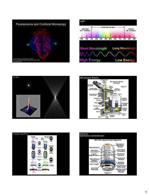
Fluorescence and Confocal Microscopy

Fluorescence and Confocal Microscopy
Joshua Nordberg and Christopher English
Olympus BioScapes Digital Imaging Competition 2004
Honorable Mention
Light:
Airy Disk Microscope Basics
Conjugate Image Planes Objectives:
Specifications and Identification
1

Objectives:
Chromatic Aberration
Objectives:
Air vs. Oil
Fluorescence
Objectives:
Numerical Apertures
Mag
Plan Achromat
(NA)
Plan Fluorite
(NA)
Plan Apochromat
(NA)
0.5x 0.025 n/a n/a
1x 0.04 n/a n/a
2x 0.06 n/a 0.10
4x 0.10 0.13 0.20
10x 0.25 0.30 0.45
20x 0.40 0.50 0.75
40x 0.65 0.75 0.95
40x (oil) n/a 1.30 1.00
60x 0.75 0.85 0.95
60x (oil) n/a n/a 1.40
100x (oil) 1.25 1.30 1.40
Objectives:
Light-Gathering Power
Correction Magnification
Numerical
Aperture
F(trans) F(epi)
Plan Achromat 10x 0.25 6.25 0.39
Plan Fluorite 10x 0.30 9.00 0.81
Plan Apo 10x 0.45 20.2 4.10
Plan Achromat 20x 0.40 4.00 0.64
Plan Fluorite 20x 0.50 6.25 1.56
Plan Apo 20x 0.75 14.0 7.90
Plan Achromat 40x 0.65 2.64 1.11
Plan Fluorite 40x 0.75 3.52 1.98
Plan Apo 40x (oil) 1.30 11.0 18.0
Plan Fluorite 60x 0.85 2.01 1.45
Plan Apo 60x (oil) 1.40 5.4 10.6
Plan Apo 100x (oil) 1.40 1.96 3.84
Plan Apo 100x (oil) 1.45 2.10 4.42
Plan Apo 100x (oil) 1.65 2.72 7.41
Hit by High
Energy Photon
e -
e -
Ground State
Excited States
Emit Low
Energy Photon
2

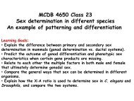
• Physical Process
– Excitation: S 0 + hv → S 1
Fluorescence
– Fluorescence (emission): S 1 → S 0 + hv
• S 0 is the ground state of the fluorophore
• S 1 is the first excited state of the fluorophore
• hν is a generic term for photon energy where:
– h = Planck’s Constant
– ν = Frequency of light
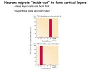
Fluorophores
Giepmans et al., 2006
Green Fluorescent Protein
• GFP was first cloned in 1992 from Aequorea
victoria by Douglas Prasher.
• Prahser also successfully expressed GFP in C.
elegans in 1994.
Fluorescence
Fluorescence Quantum Yield
– the efficiency of the fluorescence process
– Φ = # photons emitted
# photons absorbed
– The theoretical maximum fluorescence quantum
yield is 1.0 (100%) where every photon absorbed
results in a photon emitted.
RCSB Protein Data Bank
Aequorea victoria
3

Fluorescence Imaging
Transmitted (or Diascopic) illumination
Nikon (www.microscopyu.com)
Illumination Techniques
• Transmitted (or Diascopic) illumination
• Reflected (or Episcopic) illumination
Reflected (or Episcopic) Illumination
Nikon (www.microscopyu.com)
Nikon (www.microscopyu.com)
4

Nikon (www.microscopyu.com) Nikon (www.microscopyu.com)
Widefield :
Nikon (www.microscopyu.com)
Widefield :
Point Scanning:
Point Scanning:
Nikon (www.microscopyu.com)
Confocal Imaging:
• The invention of the confocal microscope is attributed
to Marvin Minsky, who produced a working
microscope in 1955.
• It was developed to eliminate out-of-focus haze of
fluorescent samples.
5

Light
Source
First
Pinhole
Condenser Sample Objective
Illumination of
a Single Point
Collection from
the Same Point
http://web.media.mit.edu/~minsky/papers/ConfocalMemoir.html
Second
Pinhole
Confocal Imaging
(its all about the pinhole)
Detector
• Any light that passed the second pinhole struck
a photomultiplier, which generated a signal that
was related to the brightness of the light from the
specimen.
• The second pinhole prevented light originating
from above or below the plane of focus in the
specimen from reaching the photomultiplier.
Spinning Disk Confocal
Confocal Imaging
(its all about the pinhole)
• Minsky's original configuration used a pinhole placed
in front of a zirconium arc source as the point source
of light.
• The point of light was focused by an objective lens at
the desired focal plane in the specimen, and light that
passed through it was focused by a second objective
lens at a second pinhole having the same focus as the
first pinhole (the two were confocal).
Confocal Systems:
• Spinning Disk Confocal Scope
• LASER Scanning Confocal Microscope
– Single Photon
• Fluorophores are excited by one photon of high(er)
energy light
– Two Photon
• Fluorophores are excited by two photon of low(er)
energy light
Laser Scanning Confocal
Nikon (www.microscopyu.com)
6

Controlling Image Quality:
• Spinning Disk Confocal Microscope
– Exposure (ms)
– Gain (software)
– Digitizer
– EM-Gain (hardware)
– Frame Averaging
• LASER Scanning Confocal Microscope
– Frame Size (X Pixels by Y Pixels)
• Pixel Size
– Scan Speed
– Pinhole Size
– Gain
– Frame Averaging
What are Digital Images
• Digital images are stored using binary code (1 or 0)
• Bit depth: potential grayscale pixel
Monochromatic Bit Depth
• 1 bit = 2 gray levels
• 2 bit = 4 gray levels
• 4 bit = 16 gray levels
• 8 bit = 256 gray levels
• 12 bit = 4,096 gray levels
• 16 bit = 65,536 gray levels
Color Images
• 24-bit RGB images
– 8-bits for each of the red, green and blue channels
Noise
1. Statistical Noise: Random fluctuations in signal
2. Dark (Thermal) Noise
•Electrons pop out of the chip as it heats up
•They build up with long exposure time
•Can be reduced by cooling chip
3. Read Out Noise
•Errors as chip is read
•Constant, regardless of exposure time
•Can be reduced by reading the chip more slowly
4. Camera Noise (Dark + Readout)
5. Total Noise (Signal noise + Camera noise)
1.25 MHz/pixel
10 MHz/pixel
Images collected by JWS in the Nikon Imaging Center at Harvard Medical School
Digital Images:
Separating Signal from Noise
Ted Hinchcliffe & Kenneth Spring
• Signal is defined as the change in the state of a detector produced by
photons from the object of interest.
• Noise is defined as meaningless fluctuations in the signal. It is of three
kinds:
• Optical Noise is defined as any detected photon produced by stray light
from the microscope or scattered from the object of interest.
• Camera Noise is defined as any change in the detector output not
produced by photons from the object of interest.
• Statistical Noise is defined as fluctuations in signal that arise from the
random changes that result from inadequate sampling.
Signal-to-noise ratio and its effect on image quality.
7

Ways to increase the signal that the camera sees
•Brighter sample
•Align illumination optics (Koehler illumination) & bulb
•Brighter objective lens (B = NA 4 / M 2 )
•Higher transmission objective lens (less aberration correction)
•Decrease specimen noise (mounting medium, BG fluorescence)
•Decrease other optical noise (minimize reflective surfaces, use
field diaphragm, work in dark, no dirt)
Detectors: Photomultiplier Tube (PMT)
Strengths: very low noise and allow rapid data collection
Weaknesses: old designs don’t count every photon (GaAs PMTs, 10%
efficient), but new PMTs GaAsP) are about 40% efficient at their spectral
optimum.
Nikon (www.microscopyu.com)
A metaphore
for CCD camera
readout
Gain:
• The amount that an analog signal has been amplified. For video, gain is used to
increase or decrease the dynamic range of a video camera by selecting the voltage
levels that the digitizer will accept.
• For example, when viewing a faint image, the gain is often raised to increase the
minute changes into those that are more readily detectable.
Increasing gain reduces the number of gray levels
Increasing gain, Same exposure time
Offset (Black Level), can be used to re-zero the gray scale
Detectors: Charged Coupled Device (CCD)
Images collected by JWS in the Nikon Imaging Center at Harvard Medical School
The sensitivities of various electronic cameras: Video - CCD
Photodiodes
• A light-sensitive semi-conductor set up so
incident light can knock electrons loose.
• A “loose” electron leaves behind a zone of
positive charge or a “hole”
• Electrons and holes can move in response to
an electric field
• Current is then proportional to the number of
“loose” electrons, i.e., to number of incident
photons
8

Diagram of an individual CCD “Well” or “Pixel”
full well capacity
on the order of ~1000 electrons/µm 2
Spectral Sensitivity & QE
Detector: Electron Multiplier CCD(EM-CCD)
Hazelwood et al., from Shorte and Frischknecht 2007
Graph from microscopyu.com
Hamamatsu
Improvements in Interline CCDs
Single microlens added
No microlens
Detector: Charged Coupled Device (CCD)
ORCA- ER
500ms, High Gain
Input
light
EM-CCD Performance
EM-CCD
200ms, Low Multiplication
Open window
EM-CCD
200ms, Med Multiplication
Microlens
Image from Butch Moomaw, Hamamatsu
Hamamatsu
EM-CCD
50ms, High Multiplication
Images collected by JWS in the Nikon Imaging Center at Harvard Medical School
9

Detector: Electron Multiplier CCD(EM-CCD)
Dangers of Converting
From 16 Bit to 8 Bit
Hamamatsu
Detector: Electron Multiplier CCD(EM-CCD)
Nakano, 2002
16 Bit 16 Bit
16 Bit 16 Bit 8 Bit 8 Bit
Hamamatsu
10

Starting Images
Ending Images
16 Bit 16 Bit
8 Bit 8 Bit
References
• Douglas C. Prasher, Virginia K. Eckenrode, William W. Ward, Frank G. Prendergast and Milton J.
Cormier. Primary structure of the Aequorea victoria green-fluorescent protein. Gene. 1992 Feb
15;111(2):229-33.
• Chalfie M, Tu Y, Euskirchen G, Ward W, and Prasher DC. Green fluorescent protein as a
marker for gene expression. Science. 1994 Feb 11;263(5148):802-5.
• Giepmans BN, Adams SR, Ellisman MH, and Tsien RY. The fluorescent toolbox for assessing
protein location and function. Science. 2006 Apr 14;312(5771):217-24.
• Shaner NC, Campbell RE, Steinbach PA, Giepmans BN, Palmer AE, and Tsien RY. Improved
monomeric red, orange and yellow fluorescent proteins derived from Discosoma sp. red
fluorescent protein. Nat Biotechnol. 2004 Dec;22(12):1567-72. Epub 2004 Nov 21.
• Semwogerere D. and Weeks ER. Confocal Microscopy Encyclopedia of Biomaterials and
Biomedical Engineering 2005 Nov. 28 10;(1-10).
• Nakano A. Spinning-disk confocal microscopy - a cutting-edge tool for imaging of membrane
traffic. Cell Struct Funct. 2002 Oct;27(5):349-55.
• Nikon Microscopy U
– http://www.microscopyu.com/index.html
11