Mathematical Modelling of Granulation: Static and Dynamic Liquid ...
Mathematical Modelling of Granulation: Static and Dynamic Liquid ...
Mathematical Modelling of Granulation: Static and Dynamic Liquid ...

You also want an ePaper? Increase the reach of your titles
YUMPU automatically turns print PDFs into web optimized ePapers that Google loves.
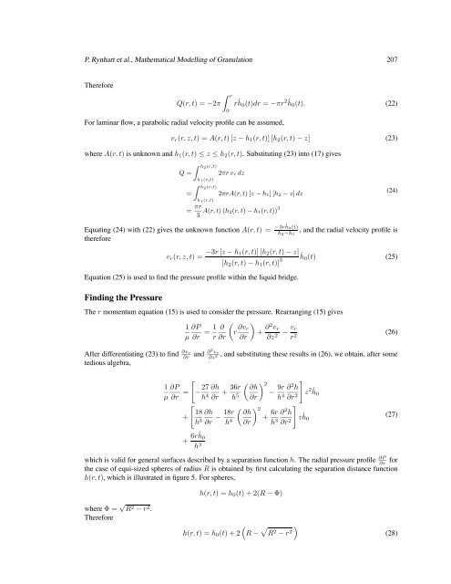
P. Rynhart et al., <strong>Mathematical</strong> <strong>Modelling</strong> <strong>of</strong> <strong>Granulation</strong> 207<br />
Therefore<br />
Q(r, t) =−2π<br />
r<br />
For laminar flow, a parabolic radial velocity pr<strong>of</strong>ile can be assumed,<br />
0<br />
r ˙ h0(t)dr = −πr 2 ˙ h0(t). (22)<br />
vr(r, z, t) =A(r, t)[z − h1(r, t)] [h2(r, t) − z] (23)<br />
where A(r, t) is unknown <strong>and</strong> h1(r, t) ≤ z ≤ h2(r, t). Substituting (23) into (17) gives<br />
Q =<br />
Z h2(r,t)<br />
h1(r,t) Z h2(r,t)<br />
2πr vr dz<br />
= 2πrA(r, t)[z − h1][h2 − z] dz<br />
h1(r,t)<br />
= πr<br />
A(r, t)(h2(r, t) − h1(r, t))3<br />
3<br />
Equating (24) with (22) gives the unknown function A(r, t) = −3r ˙ h0(t)<br />
,<strong>and</strong> the radial velocity pr<strong>of</strong>ile is<br />
h2−h1<br />
therefore<br />
vr(r, z, t) = −3r [z − h1(r, t)] [h2(r, t) − z]<br />
[h2(r, t) − h1(r, t)] 3<br />
˙h0(t) (25)<br />
Equation (25) is used to find the pressure pr<strong>of</strong>ile within the liquid bridge.<br />
Finding the Pressure<br />
The r momentum equation (15) is used to consider the pressure. Rearranging (15) gives<br />
<br />
1 ∂P 1 ∂<br />
= r<br />
µ ∂r r ∂r<br />
∂vr<br />
<br />
+<br />
∂r<br />
∂2vr vr<br />
−<br />
∂z2 r2 After differentiating (23) to find ∂vr<br />
∂r <strong>and</strong> ∂2vr ∂z2 ,<strong>and</strong> substituting these results in (26), we obtain, after some<br />
tedious algebra,<br />
1 ∂P<br />
µ<br />
∂r =<br />
+<br />
<br />
− 27<br />
h 4<br />
∂h 36r<br />
+<br />
∂r h5 <br />
18<br />
h3 ∂h 18r<br />
−<br />
∂r h4 + 6r ˙ h0<br />
h 3<br />
<br />
∂h<br />
∂r<br />
2<br />
− 9r<br />
h 4<br />
2 ∂h<br />
+<br />
∂r<br />
6r<br />
h3 ∂2h ∂r2 <br />
z 2 h0<br />
˙<br />
<br />
z ˙ h0<br />
which is valid for general surfaces described by a separation function h. Theradial pressure pr<strong>of</strong>ile ∂P<br />
∂r for<br />
the case <strong>of</strong> equi-sized spheres <strong>of</strong> radius R is obtained by first calculating the separation distance function<br />
h(r, t),which is illustrated in figure 5. For spheres,<br />
where Φ= √ R 2 − r 2 .<br />
Therefore<br />
h(r, t) =h0(t)+2(R − Φ)<br />
∂ 2 h<br />
∂r 2<br />
<br />
h(r, t) =h0(t)+2 R − R2 − r2 <br />
(24)<br />
(26)<br />
(27)<br />
(28)