Mathematical Modelling of Granulation: Static and Dynamic Liquid ...

206 R.L.I.M.S. Vol. 3, April, 2002
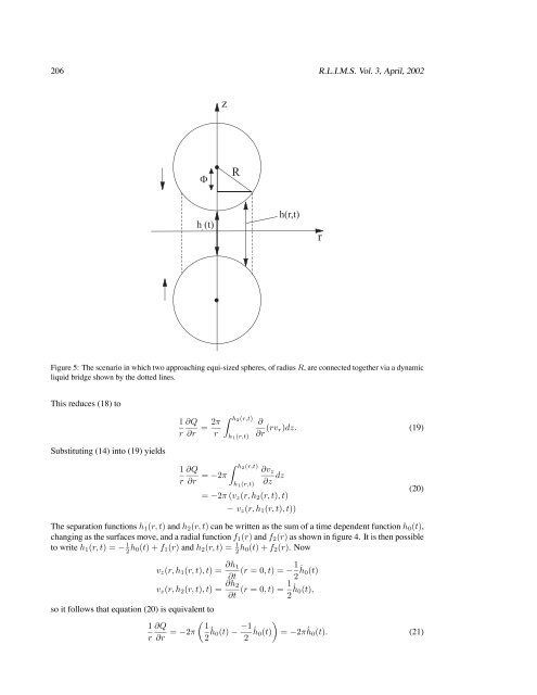
Figure 5: The scenario in which two approaching equi-sized spheres, of radius R,are connected together via a dynamic
liquid bridge shown by the dotted lines.
This reduces (18) to
Substituting (14) into (19) yields
h2(r,t)
1 ∂Q 2π ∂
=
r ∂r r h1(r,t) ∂r (rvr)dz. (19)
h2(r,t)
1 ∂Q
∂vz
= −2π
r ∂r h1(r,t) ∂z dz
= −2π (vz(r, h2(r, t),t)
− vz(r, h1(r, t),t))
The separation functions h1(r, t) and h2(r, t) can be written as the sum of a time dependent function h0(t),
changing as the surfaces move, and a radial function f1(r) and f2(r) as shown in figure 4. It is then possible
to write h1(r, t) =− 1
2 h0(t)+f1(r) and h2(r, t) = 1
2 h0(t)+f2(r). Now
so it follows that equation (20) is equivalent to
vz(r, h1(r, t),t)= ∂h1
(r =0,t)=−1
∂t 2 ˙ h0(t)
vz(r, h2(r, t),t)= ∂h2
(r =0,t)=1
∂t 2 ˙ h0(t),
1 ∂Q
= −2π
r ∂r
1
2 ˙ h0(t) − −1
2 ˙ h0(t)
(20)
= −2π ˙ h0(t). (21)