Mathematical Modelling of Granulation: Static and Dynamic Liquid ...

202 R.L.I.M.S. Vol. 3, April, 2002
φ
100
80
60
40
20
0
−20
−40
−60
−80
0.5
0.4
0.3
0.1
0.2
0
−100
0 0.5 1 1.5 2 2.5
R ∆ P
3 3.5 4 4.5 5
where
and
−1
−2
−3
−4
−5
−6
−7
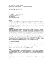
Figure 2: Phase portrait for ∆P >0. Hereφ = arctan R ′ . Contour labels are values of E ∆P .
η 2 ,ξ 2 =
2
(∆P ) 2
(1 − E∆P ± √
1 − 2E∆P
ξ = χ/η
such that ξ ≤ R ≤ η,andwhere E and F are Jacobi elliptic functions of the first kind [9]. Equation (11) defines
the shape (R) ofabridge parameterised by the position X, wheretheenergylevels E are determined
from (8). Upon consideration of the discriminant of the the quadratic in X 2 of (9), it can be shown that
E ∆P < 1
2 .
Although equation (11) represents the liquid bridge configuration in terms of known mathematical functions,
difficulty arises when attempting to integrate this solution to determine properties such as the bridge surface
area and volume. In order to solve the problem in which certain properties are held constant, approximations
to the bridge surface, or a numerical scheme, must be used (as in [2-6]).
Phase Portrait
The energy level E is related to the height and slope of the bridge surface (R, R ′ )byequation (8). Boundary
conditions on R and R ′ , along with the pressure difference ∆P determine the contour for a particular liquid
bridge. Generic contours, characterising all liquid bridge configurations, can be obtained from (8) by scaling.
Upon introducing ˜ R = R ∆P and ˜ X = X ∆P ,itfollows that
E ∆P = ˜ ⎛
R ⎝
1
1+ ˜ R ′2
− ˜ ⎞
R
⎠ .
2
(12)
An angle φ measured with respect to the horizontal coordinate X is introduced where R ′
= tan φ and therefore
1+R ′2
= sec φ. Interms of φ,equation (12) becomes
E ∆P = ˜
R cos φ − ˜
R
2
for ∆P >0, (13a)