Mathematical Modelling of Granulation: Static and Dynamic Liquid ...
Mathematical Modelling of Granulation: Static and Dynamic Liquid ...
Mathematical Modelling of Granulation: Static and Dynamic Liquid ...

You also want an ePaper? Increase the reach of your titles
YUMPU automatically turns print PDFs into web optimized ePapers that Google loves.
P. Rynhart et al., <strong>Mathematical</strong> <strong>Modelling</strong> <strong>of</strong> <strong>Granulation</strong> 201<br />
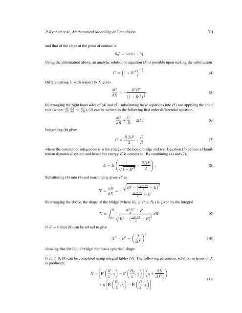
<strong>and</strong> that <strong>of</strong> the slope at the point <strong>of</strong> contact is<br />
R0 ′ = cot(α + θ).<br />
Using the information above, an analytic solution to equation (3) is possible upon making the substitution<br />
Differentiating U with respect to X gives<br />
U =<br />
<br />
1+R ′2 − 1<br />
2<br />
. (4)<br />
dU<br />
dX = − R′ R ′′<br />
3 . (5)<br />
1+R ′2 2<br />
Rearranging the right h<strong>and</strong> sides <strong>of</strong> (4) <strong>and</strong> (5), substituting these equations into (5) <strong>and</strong> applying the chain<br />
), (3) can be written as the following first order differential equation,<br />
rule (where dU dX<br />
dX dR<br />
Integrating (6) gives<br />
= dU<br />
dR<br />
dU U<br />
+ =∆P. (6)<br />
dR R<br />
U =<br />
R ∆P<br />
2<br />
where the constant <strong>of</strong> integration E is the energy <strong>of</strong> the liquid bridge surface. Equation (3) defines a Hamiltonian<br />
dynamical system <strong>and</strong> hence the energy E is conserved. By combining (4) <strong>and</strong> (7),<br />
<br />
<br />
E = R<br />
1 R∆P<br />
−<br />
1+R ′2 2<br />
. (8)<br />
Substituting (4) into (7) <strong>and</strong> rearranging gives R ′ as<br />
R ′ = dR<br />
dX<br />
= ±<br />
+ E<br />
R<br />
<br />
R2 − ∆PR2 + E2<br />
∆P R 2<br />
2<br />
2<br />
+ E<br />
Rearranging the above, the shape <strong>of</strong> the bridge (where R0 ≤ R ≤ R1)isgivenby the integral<br />
X =<br />
If E =0then (9) can be solved to give<br />
R<br />
R0<br />
<br />
∆PR 2<br />
2<br />
+ E<br />
R 2 − ∆PR 2<br />
2<br />
X 2 + R 2 2 2<br />
=<br />
∆P<br />
showing that the liquid bridge then has a spherical shape.<br />
(7)<br />
+ E2 dR. (9)<br />
If E = 0, (9) can be completed using integral tables [9]. The following parametric solution in terms <strong>of</strong> X<br />
is produced,<br />
<br />
R<br />
X = F<br />
ξ ,χ<br />
<br />
R0<br />
− F<br />
ξ ,χ<br />
<br />
η + 2E<br />
<br />
∆P η<br />
<br />
R0<br />
+ η E<br />
ξ ,χ<br />
<br />
R<br />
− E<br />
ξ ,χ<br />
(11)<br />
(10)