Mathematical Modelling of Granulation: Static and Dynamic Liquid ...
Mathematical Modelling of Granulation: Static and Dynamic Liquid ...
Mathematical Modelling of Granulation: Static and Dynamic Liquid ...

Create successful ePaper yourself
Turn your PDF publications into a flip-book with our unique Google optimized e-Paper software.
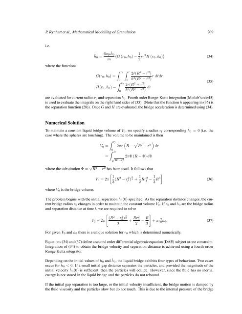
P. Rynhart et al., <strong>Mathematical</strong> <strong>Modelling</strong> <strong>of</strong> <strong>Granulation</strong> 209<br />
i.e.<br />
where the functions<br />
¨h0 = 6πµ˙ h0<br />
m {G (r0,h0) − 1<br />
2 r0 2 H (r0,h0)} (34)<br />
G(r0,h0) =<br />
H(r0,h0) =<br />
r0 r<br />
2ˆr(R<br />
0 0<br />
2 +ˆr 2 )<br />
h3 (R2 − ˆr 2 ) rdˆrdr<br />
r0<br />
2r(R<br />
0<br />
2 + r2 )<br />
h3 (R2 − r2 ) dr<br />
are evaluated for current radius r0 <strong>and</strong> separation h0. Fourth order Runge-Kutta integration (Matlab’s ode45)<br />
is used to evaluate the integrals on the right h<strong>and</strong> sides <strong>of</strong> (35). (Note that the function h appearing in (35) is<br />
the separation function (28)). Once G <strong>and</strong> H are evaluated, the bridge acceleration is determined using (34).<br />
Numerical Solution<br />
To maintain a constant liquid bridge volume <strong>of</strong> V0, wespecify a radius rf corresponding h0 =0(i.e. the<br />
case where the spheres are touching). The volume to be maintained is then<br />
V0 =<br />
=<br />
rf<br />
0 R<br />
<br />
2πr R − R2 − r2 <br />
dr<br />
√ R 2 −r 2 f<br />
2πΦ(R − Φ) dΦ<br />
where the substitution Φ= √ R 2 − r 2 has been used. It follows that<br />
where V0 is the bridge volume.<br />
V0 =2π<br />
<br />
1<br />
3 (R2 − r 2 f ) 3<br />
2 + 1<br />
2 Rr2 f − 1<br />
3 R3<br />
<br />
The problem begins with the initial separation h0(0) specified. As the separation distance changes, the current<br />
bridge radius r0 changes in order to maintain the constant volume V0. Ifr0<strong>and</strong> h0 are the bridge radius<br />
<strong>and</strong> separation distance at time t, wearerequired to solve<br />
V0 =2π<br />
<br />
(R2 − r2 0) 3<br />
2<br />
3<br />
+ Rr2 0<br />
2<br />
(35)<br />
(36)<br />
<br />
R<br />
−<br />
3<br />
+ πr 2 0h0. (37)<br />
For given V0 <strong>and</strong> h0 there is a unique solution for r0 which is determined numerically.<br />
Equations (34) <strong>and</strong> (37) define a second order differential algebraic equation (DAE) subject to one constraint.<br />
Integration <strong>of</strong> (34) to obtain the bridge velocity <strong>and</strong> separation distance is achieved using a fourth order<br />
Runge Kutta integrator.<br />
Depending on the initial values <strong>of</strong> h0 <strong>and</strong> ˙ h0, theliquid bridge exhibits four types <strong>of</strong> behaviour. Two cases<br />
occur for ˙ h0 < 0. Ifasmall initial gap distance separates the particles, <strong>and</strong> provided the magnitude <strong>of</strong> the<br />
initial velocity ˙ h0(0) is sufficient, then the particles will collide. However, since the fluid has no inertia,<br />
energy is not stored in the liquid bridge <strong>and</strong> the particles do not rebound.<br />
If the initial gap separation is too large, or the initial velocity insufficient, the bridge motion is damped by<br />
the fluid viscosity <strong>and</strong> the particles slow but do not touch. This is due to the internal pressure <strong>of</strong> the bridge