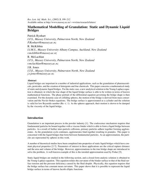
Mathematical Modelling of Granulation: Static and Dynamic Liquid ...
Mathematical Modelling of Granulation: Static and Dynamic Liquid ...
Mathematical Modelling of Granulation: Static and Dynamic Liquid ...

Create successful ePaper yourself
Turn your PDF publications into a flip-book with our unique Google optimized e-Paper software.
Res. Lett. Inf. Math. Sci., (2002) 3, 199–212<br />
Available online at http://www.massey.ac.nz/∼wwiims/research/letters/<br />
<strong>Mathematical</strong> <strong>Modelling</strong> <strong>of</strong> <strong>Granulation</strong>: <strong>Static</strong> <strong>and</strong> <strong>Dynamic</strong> <strong>Liquid</strong><br />
Bridges<br />
Patrick Rynhart<br />
I.F.S., Massey University, Palmerston North, New Zeal<strong>and</strong><br />
P.Rynhart@massey.ac.nz<br />
R. McKibbin<br />
I.I.M.S., Massey University Albany Campus, Auckl<strong>and</strong>, New Zeal<strong>and</strong><br />
r.mckibbin@massey.ac.nz<br />
R. McLachlan<br />
I.F.S., Massey University, Palmerston North, New Zeal<strong>and</strong><br />
r.mclachlan@massey.ac.nz<br />
J.R. Jones<br />
I.T.E., Massey University, Palmerston North, New Zeal<strong>and</strong><br />
j.r.jones@massey.ac.nz<br />
Abstract<br />
<strong>Liquid</strong> bridges are important in a number <strong>of</strong> industrial applications, such as the granulation <strong>of</strong> pharmaceuticals,<br />
pesticides, <strong>and</strong> the creation <strong>of</strong> detergents <strong>and</strong> fine chemicals. This paper concerns a mathematical study<br />
<strong>of</strong> static <strong>and</strong> dynamic liquid bridges. For the static case, a new analytical solution to the Young-Laplace equation<br />
is obtained, in which the true shape <strong>of</strong> the liquid bridge surface is able to be written in terms <strong>of</strong> known<br />
mathematical functions. The phase portrait <strong>of</strong> the differential equation governing the bridge shape is then<br />
examined. For the dynamic case <strong>of</strong> colliding spheres, the motion <strong>of</strong> the bridge is derived from mass conservation<br />
<strong>and</strong> the Navier-Stokes equations. The bridge surface is approximated as a cylinder <strong>and</strong> the solution<br />
is valid for low Reynolds number (Re ≪ 1). As the spheres approach, their motion is shown to be damped<br />
by the viscosity <strong>of</strong> the liquid bridge.<br />
Introduction<br />
<strong>Granulation</strong> is an important process in the powder industry [1]. The coalescence mechanism requires that<br />
fundamental particles be bound together with a viscous binder which is able to form a liquid bridge between<br />
particles. As a result <strong>of</strong> further inter-particle collisions, primary particles adhere together forming agglomerates.<br />
As the granulation cycle continues, agglomerates bind together resulting in granules. This paper is<br />
concerned with the liquid bridges that form between fundamental particles. As an approximation, the particles<br />
are represented by spheres in this work.<br />
A number <strong>of</strong> theoretical studies have been completed into properties <strong>of</strong> static liquid bridges which have constant<br />
physical properties [2-7]. Parameters <strong>of</strong> interest in these applications are the critical rupture distance<br />
<strong>and</strong> the area <strong>and</strong> volume <strong>of</strong> the bridge. However, approximations to the true bridge shape are introduced to<br />
solve the problem. A well-known example <strong>of</strong> this is the toroidal approximation used by Fisher [5].<br />
<strong>Static</strong> liquid bridges are studied in the following section, <strong>and</strong> a closed form analytic solution is obtained to<br />
the Young-Laplace equation. This equation relates the curvature <strong>of</strong> the binder surface to that <strong>of</strong> the fluid surface<br />
tension <strong>and</strong> the pressure deficiency caused by the fluid droplet. Physically, this equation requires that<br />
the bridge surface has constant mean curvature. This paper shows that it is possible to represent the liquid<br />
bridge surface in terms <strong>of</strong> known Jacobi elliptic functions.
200 R.L.I.M.S. Vol. 3, April, 2002<br />
Figure 1: Illustration <strong>of</strong> the static liquid bridge geometry. Dimensional variables are used (as in equations (1) <strong>and</strong> (2)).<br />
Acontact angle <strong>of</strong> θ =10 o , α =40 o , β =38 o .The radius <strong>of</strong> particle A is rA =0.1 mm <strong>and</strong> particle B rB =0.15 mm.<br />
The length <strong>of</strong> the bridge is 0.12 mm.<br />
<strong>Static</strong> Bridges<br />
Consider figure 1 which illustrates a liquid bridge with cylindrical symmetry between two spherical particles<br />
‘A’ <strong>and</strong> ‘B’ <strong>of</strong> radii rA <strong>and</strong> rB. Coordinates r <strong>and</strong> x define the position <strong>of</strong> the liquid bridge surface along<br />
with the radii <strong>of</strong> curvature r1 <strong>and</strong> r2 which lie in the r − x <strong>and</strong> r − y planes respectively. The curvature<br />
in the r-x plane is therefore given by 1<br />
1<br />
,<strong>and</strong>thecurvature in the r-y plane by .Allowing ∆p to denote<br />
r1 r2<br />
the pressure deficiency caused by the presence <strong>of</strong> the liquid droplet (∆p >0 when the internal pressure <strong>of</strong><br />
the bridge is higher than the external (ambient) pressure), the Young-Laplace equation relates the surface<br />
tension <strong>of</strong> the binder γ to the pressure difference ∆p <strong>and</strong> the mean curvature <strong>of</strong> the bridge surface,<br />
<br />
1<br />
γ +<br />
r1<br />
1<br />
<br />
=∆p. (1)<br />
r2<br />
Gravity does not appear in (1) as the mass <strong>of</strong> the liquid bridge is very small in comparison with the surface<br />
tension force between particles. Upon substitution <strong>of</strong> the vector calculus results for 1 1 <strong>and</strong> (see [8] for<br />
r1 r2<br />
details), equation (1) can be written<br />
<br />
<br />
1<br />
γ<br />
= −∆p. (2)<br />
r ′′<br />
(1 + r ′2 ) 3/2 −<br />
r(1 + r ′2 ) 1/2<br />
Equation (2) can be non-dimensionalised by introducing variables X = x<br />
r<br />
σ <strong>and</strong> R = σ ,where σ is the scaling<br />
variable relating non-dimensional <strong>and</strong> dimensional variables. In the case <strong>of</strong> figure 1, σ can be chosen as<br />
either rA or rB. Also, a non-dimensional pressure difference ∆P = ∆pσ<br />
γ is introduced, enabling the nondimensional<br />
version <strong>of</strong> (2) to be written as<br />
R ′′<br />
(1 + R ′2<br />
) 3/2 −<br />
1<br />
R(1 + R ′2 = −∆P. (3)<br />
) 1/2<br />
In (3) the notation R ′ = dR<br />
dX <strong>and</strong> R′′ = d2R dX2 has been adopted. Initial values for the bridge height R0 <strong>and</strong><br />
tangent R ′ 0 (occurring on particle A above) are specified. The angle which the bridge makes contact with the<br />
tangent plane to the spheres is the contact angle θ <strong>and</strong> is specified for a given problem. The starting value<br />
for the bridge height (occurring at X0)is<br />
R0 = rA<br />
σ sin α = RA sin α
P. Rynhart et al., <strong>Mathematical</strong> <strong>Modelling</strong> <strong>of</strong> <strong>Granulation</strong> 201<br />
<strong>and</strong> that <strong>of</strong> the slope at the point <strong>of</strong> contact is<br />
R0 ′ = cot(α + θ).<br />
Using the information above, an analytic solution to equation (3) is possible upon making the substitution<br />
Differentiating U with respect to X gives<br />
U =<br />
<br />
1+R ′2 − 1<br />
2<br />
. (4)<br />
dU<br />
dX = − R′ R ′′<br />
3 . (5)<br />
1+R ′2 2<br />
Rearranging the right h<strong>and</strong> sides <strong>of</strong> (4) <strong>and</strong> (5), substituting these equations into (5) <strong>and</strong> applying the chain<br />
), (3) can be written as the following first order differential equation,<br />
rule (where dU dX<br />
dX dR<br />
Integrating (6) gives<br />
= dU<br />
dR<br />
dU U<br />
+ =∆P. (6)<br />
dR R<br />
U =<br />
R ∆P<br />
2<br />
where the constant <strong>of</strong> integration E is the energy <strong>of</strong> the liquid bridge surface. Equation (3) defines a Hamiltonian<br />
dynamical system <strong>and</strong> hence the energy E is conserved. By combining (4) <strong>and</strong> (7),<br />
<br />
<br />
E = R<br />
1 R∆P<br />
−<br />
1+R ′2 2<br />
. (8)<br />
Substituting (4) into (7) <strong>and</strong> rearranging gives R ′ as<br />
R ′ = dR<br />
dX<br />
= ±<br />
+ E<br />
R<br />
<br />
R2 − ∆PR2 + E2<br />
∆P R 2<br />
2<br />
2<br />
+ E<br />
Rearranging the above, the shape <strong>of</strong> the bridge (where R0 ≤ R ≤ R1)isgivenby the integral<br />
X =<br />
If E =0then (9) can be solved to give<br />
R<br />
R0<br />
<br />
∆PR 2<br />
2<br />
+ E<br />
R 2 − ∆PR 2<br />
2<br />
X 2 + R 2 2 2<br />
=<br />
∆P<br />
showing that the liquid bridge then has a spherical shape.<br />
(7)<br />
+ E2 dR. (9)<br />
If E = 0, (9) can be completed using integral tables [9]. The following parametric solution in terms <strong>of</strong> X<br />
is produced,<br />
<br />
R<br />
X = F<br />
ξ ,χ<br />
<br />
R0<br />
− F<br />
ξ ,χ<br />
<br />
η + 2E<br />
<br />
∆P η<br />
<br />
R0<br />
+ η E<br />
ξ ,χ<br />
<br />
R<br />
− E<br />
ξ ,χ<br />
(11)<br />
(10)
202 R.L.I.M.S. Vol. 3, April, 2002<br />
φ<br />
100<br />
80<br />
60<br />
40<br />
20<br />
0<br />
−20<br />
−40<br />
−60<br />
−80<br />
0.5<br />
0.4<br />
0.3<br />
0.1<br />
0.2<br />
0<br />
−100<br />
0 0.5 1 1.5 2 2.5<br />
R ∆ P<br />
3 3.5 4 4.5 5<br />
where<br />
<strong>and</strong><br />
−1<br />
−2<br />
−3<br />
−4<br />
−5<br />
−6<br />
−7<br />
Figure 2: Phase portrait for ∆P >0. Hereφ = arctan R ′ . Contour labels are values <strong>of</strong> E ∆P .<br />
η 2 ,ξ 2 =<br />
2<br />
(∆P ) 2<br />
<br />
(1 − E∆P ± √ <br />
1 − 2E∆P<br />
ξ = χ/η<br />
such that ξ ≤ R ≤ η,<strong>and</strong>where E <strong>and</strong> F are Jacobi elliptic functions <strong>of</strong> the first kind [9]. Equation (11) defines<br />
the shape (R) <strong>of</strong>abridge parameterised by the position X, wheretheenergylevels E are determined<br />
from (8). Upon consideration <strong>of</strong> the discriminant <strong>of</strong> the the quadratic in X 2 <strong>of</strong> (9), it can be shown that<br />
E ∆P < 1<br />
2 .<br />
Although equation (11) represents the liquid bridge configuration in terms <strong>of</strong> known mathematical functions,<br />
difficulty arises when attempting to integrate this solution to determine properties such as the bridge surface<br />
area <strong>and</strong> volume. In order to solve the problem in which certain properties are held constant, approximations<br />
to the bridge surface, or a numerical scheme, must be used (as in [2-6]).<br />
Phase Portrait<br />
The energy level E is related to the height <strong>and</strong> slope <strong>of</strong> the bridge surface (R, R ′ )byequation (8). Boundary<br />
conditions on R <strong>and</strong> R ′ , along with the pressure difference ∆P determine the contour for a particular liquid<br />
bridge. Generic contours, characterising all liquid bridge configurations, can be obtained from (8) by scaling.<br />
Upon introducing ˜ R = R ∆P <strong>and</strong> ˜ X = X ∆P ,itfollows that<br />
E ∆P = ˜ ⎛<br />
R ⎝<br />
1<br />
<br />
1+ ˜ R ′2<br />
− ˜ ⎞<br />
R<br />
⎠ .<br />
2<br />
(12)<br />
An angle φ measured with respect to the horizontal coordinate X is introduced where R ′ <br />
= tan φ <strong>and</strong> therefore<br />
1+R ′2<br />
= sec φ. Interms <strong>of</strong> φ,equation (12) becomes<br />
E ∆P = ˜ <br />
R cos φ − ˜ <br />
R<br />
2<br />
for ∆P >0, (13a)
P. Rynhart et al., <strong>Mathematical</strong> <strong>Modelling</strong> <strong>of</strong> <strong>Granulation</strong> 203<br />
φ<br />
100<br />
0<br />
80<br />
60<br />
40<br />
20<br />
0<br />
−20<br />
−40<br />
−60<br />
−80<br />
0<br />
1 2<br />
3<br />
−100<br />
0 0.5 1 1.5 2 2.5<br />
R ∆ P<br />
3 3.5 4 4.5 5<br />
φ<br />
(a) Phase portrait for ∆P
204 R.L.I.M.S. Vol. 3, April, 2002<br />
<strong>and</strong><br />
E ∆P = ˜ <br />
R cos φ + ˜ <br />
R<br />
2<br />
for ∆P 0, periodic solutions exist<br />
for |φ| < 90 o .Forthiscase, the shape <strong>of</strong> the liquid surface is that <strong>of</strong> a ‘wavy’ cylinder. For the contour<br />
E ∆P =0.5, φ ≡ 0 o <strong>and</strong> this corresponds to the cylinder solution. For E ∆P < 0, theliquid surface<br />
begins with initial height R0, <strong>and</strong> curves upwards reaching a maximum height Rmax >R0. The critical<br />
contour at φ =90 o (E ∆P =0)isthe sphere described in (10), which separates the cylinder <strong>and</strong> upwardly<br />
curved solutions.<br />
When the pressure inside the bridge is equal to the external (ambient) pressure (as in figure 3(b)), two types<br />
<strong>of</strong> liquid bridges occur : for |φ| = 90 o ,the bridges start with initial height R0 <strong>and</strong> then curve inward achieving<br />
a height Rmin
P. Rynhart et al., <strong>Mathematical</strong> <strong>Modelling</strong> <strong>of</strong> <strong>Granulation</strong> 205<br />
Neglecting inertial terms, that is assuming Re ≪ 1, the momentum equations from [11] reduce to<br />
0=− ∂P<br />
∂r + µ ∂2vr 1 ∂vr<br />
+<br />
∂r2 r ∂r + ∂2vr ∂z<br />
0=− ∂P<br />
∂z − ρg + µ ∂2vz 1<br />
+<br />
∂r2 r<br />
r 2<br />
2 − vr<br />
∂vz<br />
∂r + ∂2vz ∂z2 where P = P (r, z) is the pressure difference between the inside <strong>and</strong> outside <strong>of</strong> the liquid bridge, defined<br />
to be positive when the pressure is higher internally. To make progress on this problem, an approximation<br />
that vz ≪ vr is introduced. Physically this means that the bridges must have a small volume, <strong>and</strong> that a<br />
small gap distance h must separate the particles when compared to the volume <strong>and</strong> radius <strong>of</strong> a fundamental<br />
particle with radius R. Since vz ≪ vr, <strong>and</strong> because gravity is not considered in this approximation, only<br />
equation (15) is applicable to the solution.<br />
Figure 4: Figure showing two general surfaces that are approaching each other, described by z1 = h1(r, t) <strong>and</strong> z2 =<br />
h2(r, t), separated by a distance h0(t) which is the distance <strong>of</strong> closest approach between the two surfaces.<br />
Velocity Pr<strong>of</strong>ile<br />
Consider the volume flow rate Q <strong>of</strong> fluid displaced when surfaces z1 <strong>and</strong> z2 move toward each other. Since<br />
the surfaces have cylindrical symmetry,<br />
Q =<br />
h2(r,t)<br />
h1(r,t)<br />
(15)<br />
(16)<br />
2πr vr dz. (17)<br />
To determine Q,wemanipulate (17) by taking the partial derivative <strong>of</strong> Q with respect to r,<strong>and</strong>then dividing<br />
through by r. Upon completing this, we obtain<br />
1<br />
r<br />
∂<br />
∂r<br />
+ 2π<br />
r<br />
Z h2(r,t)<br />
h1(r,t)<br />
∂h2<br />
∂r<br />
! 2π<br />
2πrvr dz =<br />
r<br />
Z h2(r,t)<br />
h1(r,t)<br />
∂<br />
∂r (rvr)dz<br />
∂h1<br />
vr(r, h2(r, t),t) − vr(r, h1(r, t),t)<br />
∂r<br />
where the second term in (18) arises upon application <strong>of</strong> the fundamental theorem <strong>of</strong> calculus <strong>and</strong> the chain<br />
rule. Now, since the fluid is unable to move through the surfaces,<br />
vr(r, h1(r, t),t)=vr(r, h2(r, t),t)=0.<br />
(18)
206 R.L.I.M.S. Vol. 3, April, 2002<br />
Figure 5: The scenario in which two approaching equi-sized spheres, <strong>of</strong> radius R,are connected together via a dynamic<br />
liquid bridge shown by the dotted lines.<br />
This reduces (18) to<br />
Substituting (14) into (19) yields<br />
h2(r,t)<br />
1 ∂Q 2π ∂<br />
=<br />
r ∂r r h1(r,t) ∂r (rvr)dz. (19)<br />
h2(r,t)<br />
1 ∂Q<br />
∂vz<br />
= −2π<br />
r ∂r h1(r,t) ∂z dz<br />
= −2π (vz(r, h2(r, t),t)<br />
− vz(r, h1(r, t),t))<br />
The separation functions h1(r, t) <strong>and</strong> h2(r, t) can be written as the sum <strong>of</strong> a time dependent function h0(t),<br />
changing as the surfaces move, <strong>and</strong> a radial function f1(r) <strong>and</strong> f2(r) as shown in figure 4. It is then possible<br />
to write h1(r, t) =− 1<br />
2 h0(t)+f1(r) <strong>and</strong> h2(r, t) = 1<br />
2 h0(t)+f2(r). Now<br />
so it follows that equation (20) is equivalent to<br />
vz(r, h1(r, t),t)= ∂h1<br />
(r =0,t)=−1<br />
∂t 2 ˙ h0(t)<br />
vz(r, h2(r, t),t)= ∂h2<br />
(r =0,t)=1<br />
∂t 2 ˙ h0(t),<br />
1 ∂Q<br />
= −2π<br />
r ∂r<br />
1<br />
2 ˙ h0(t) − −1<br />
2 ˙ h0(t)<br />
(20)<br />
<br />
= −2π ˙ h0(t). (21)
P. Rynhart et al., <strong>Mathematical</strong> <strong>Modelling</strong> <strong>of</strong> <strong>Granulation</strong> 207<br />
Therefore<br />
Q(r, t) =−2π<br />
r<br />
For laminar flow, a parabolic radial velocity pr<strong>of</strong>ile can be assumed,<br />
0<br />
r ˙ h0(t)dr = −πr 2 ˙ h0(t). (22)<br />
vr(r, z, t) =A(r, t)[z − h1(r, t)] [h2(r, t) − z] (23)<br />
where A(r, t) is unknown <strong>and</strong> h1(r, t) ≤ z ≤ h2(r, t). Substituting (23) into (17) gives<br />
Q =<br />
Z h2(r,t)<br />
h1(r,t) Z h2(r,t)<br />
2πr vr dz<br />
= 2πrA(r, t)[z − h1][h2 − z] dz<br />
h1(r,t)<br />
= πr<br />
A(r, t)(h2(r, t) − h1(r, t))3<br />
3<br />
Equating (24) with (22) gives the unknown function A(r, t) = −3r ˙ h0(t)<br />
,<strong>and</strong> the radial velocity pr<strong>of</strong>ile is<br />
h2−h1<br />
therefore<br />
vr(r, z, t) = −3r [z − h1(r, t)] [h2(r, t) − z]<br />
[h2(r, t) − h1(r, t)] 3<br />
˙h0(t) (25)<br />
Equation (25) is used to find the pressure pr<strong>of</strong>ile within the liquid bridge.<br />
Finding the Pressure<br />
The r momentum equation (15) is used to consider the pressure. Rearranging (15) gives<br />
<br />
1 ∂P 1 ∂<br />
= r<br />
µ ∂r r ∂r<br />
∂vr<br />
<br />
+<br />
∂r<br />
∂2vr vr<br />
−<br />
∂z2 r2 After differentiating (23) to find ∂vr<br />
∂r <strong>and</strong> ∂2vr ∂z2 ,<strong>and</strong> substituting these results in (26), we obtain, after some<br />
tedious algebra,<br />
1 ∂P<br />
µ<br />
∂r =<br />
+<br />
<br />
− 27<br />
h 4<br />
∂h 36r<br />
+<br />
∂r h5 <br />
18<br />
h3 ∂h 18r<br />
−<br />
∂r h4 + 6r ˙ h0<br />
h 3<br />
<br />
∂h<br />
∂r<br />
2<br />
− 9r<br />
h 4<br />
2 ∂h<br />
+<br />
∂r<br />
6r<br />
h3 ∂2h ∂r2 <br />
z 2 h0<br />
˙<br />
<br />
z ˙ h0<br />
which is valid for general surfaces described by a separation function h. Theradial pressure pr<strong>of</strong>ile ∂P<br />
∂r for<br />
the case <strong>of</strong> equi-sized spheres <strong>of</strong> radius R is obtained by first calculating the separation distance function<br />
h(r, t),which is illustrated in figure 5. For spheres,<br />
where Φ= √ R 2 − r 2 .<br />
Therefore<br />
h(r, t) =h0(t)+2(R − Φ)<br />
∂ 2 h<br />
∂r 2<br />
<br />
h(r, t) =h0(t)+2 R − R2 − r2 <br />
(24)<br />
(26)<br />
(27)<br />
(28)
208 R.L.I.M.S. Vol. 3, April, 2002<br />
Differentiating (28) gives ∂h<br />
∂r = 2r √<br />
R2−r2 <strong>and</strong> ∂2h ∂r2 = 2R2<br />
(R2−r2 ) 3 .Substituting these into (27) gives<br />
2<br />
1 ∂P<br />
µ ∂r =<br />
+<br />
˙h0<br />
(R2 − r2 ) 3 2 h3 54r 3 − 72rR 2<br />
h<br />
; 2 3<br />
28rR − 36r z<br />
r 3<br />
(R2 − r2 )h4 h144h0z ˙ 2<br />
− 72zh0 ˙<br />
#<br />
z 2 +<br />
i + 6r<br />
Equation (29) includes z terms <strong>and</strong> this makes integration difficult to find the pressure P .However, since<br />
the fluid layer is small in comparison to R,the vertically averaged pressure ¯ P provides an accurate approximation.<br />
Vertical averaging, given by<br />
∂ ¯ P<br />
∂r<br />
h 3 ˙ h0<br />
(29)<br />
h(r,t)<br />
1 ∂P<br />
= dz, (30)<br />
h 0 ∂r<br />
removes the explicit z dependence, <strong>and</strong> integration to find ¯ P is then straightforward. Substitution <strong>of</strong> (29)<br />
into (30) <strong>and</strong> integrating gives<br />
∂ ¯ P<br />
∂r = 6rµ(R2 + r 2 )<br />
h 3 (R 2 − r 2 ) ˙ h0. (31)<br />
If the pressure <strong>of</strong> the liquid bridge at some r = r0 is at ambient pressure Pamb,<strong>and</strong>then the bridge exp<strong>and</strong>s<br />
to r>r0 then vertically averaged pressure is<br />
<strong>and</strong> the pressure difference<br />
Force<br />
r<br />
¯P (r, t) =Pamb +<br />
r0<br />
∂ ¯ P<br />
∂r dr<br />
= Pamb +6µ ˙ h0(t)<br />
r<br />
r0<br />
¯P (r, t) − Pamb =6µ ˙ r<br />
h0(t)<br />
r0<br />
r(R 2 + r 2 )<br />
h 3 (R 2 − r 2 ) dr,<br />
r(R2 + r2 )<br />
h3 (R2 − r2 dr. (32)<br />
)<br />
The pressure difference between the internal <strong>and</strong> external regions <strong>of</strong> the liquid bridge, ¯ P (r, t) − Pamb, provides<br />
the force which decelerates the particles.<br />
The force Fbridge is given by integrating the pressure difference over the cross-sectional area <strong>of</strong> the liquid<br />
bridge. Using equation (32), the force is<br />
Z r0<br />
Fbridge = m¨ h0(t)<br />
; = ¯P (r, t) − Pamb dA<br />
0 Z r0<br />
= 2πˆr 6µ<br />
0<br />
˙ Z r ˆr(R<br />
h0(t)<br />
r0<br />
2 +ˆr 2 )<br />
h3 (R2 − ˆr 2 dr r dˆrdr<br />
)<br />
=6πµ ˙ Z r0 Z r 2ˆr(R<br />
h0<br />
0 0<br />
2 +ˆr 2 )<br />
h3 (R2 − ˆr 2 ) rdˆrdr<br />
Z r0 Z r0 2ˆr(R<br />
− rdr<br />
0<br />
0<br />
2 +ˆr 2 )<br />
h3 (R2 − ˆr 2 ) dˆr<br />
(33)
P. Rynhart et al., <strong>Mathematical</strong> <strong>Modelling</strong> <strong>of</strong> <strong>Granulation</strong> 209<br />
i.e.<br />
where the functions<br />
¨h0 = 6πµ˙ h0<br />
m {G (r0,h0) − 1<br />
2 r0 2 H (r0,h0)} (34)<br />
G(r0,h0) =<br />
H(r0,h0) =<br />
r0 r<br />
2ˆr(R<br />
0 0<br />
2 +ˆr 2 )<br />
h3 (R2 − ˆr 2 ) rdˆrdr<br />
r0<br />
2r(R<br />
0<br />
2 + r2 )<br />
h3 (R2 − r2 ) dr<br />
are evaluated for current radius r0 <strong>and</strong> separation h0. Fourth order Runge-Kutta integration (Matlab’s ode45)<br />
is used to evaluate the integrals on the right h<strong>and</strong> sides <strong>of</strong> (35). (Note that the function h appearing in (35) is<br />
the separation function (28)). Once G <strong>and</strong> H are evaluated, the bridge acceleration is determined using (34).<br />
Numerical Solution<br />
To maintain a constant liquid bridge volume <strong>of</strong> V0, wespecify a radius rf corresponding h0 =0(i.e. the<br />
case where the spheres are touching). The volume to be maintained is then<br />
V0 =<br />
=<br />
rf<br />
0 R<br />
<br />
2πr R − R2 − r2 <br />
dr<br />
√ R 2 −r 2 f<br />
2πΦ(R − Φ) dΦ<br />
where the substitution Φ= √ R 2 − r 2 has been used. It follows that<br />
where V0 is the bridge volume.<br />
V0 =2π<br />
<br />
1<br />
3 (R2 − r 2 f ) 3<br />
2 + 1<br />
2 Rr2 f − 1<br />
3 R3<br />
<br />
The problem begins with the initial separation h0(0) specified. As the separation distance changes, the current<br />
bridge radius r0 changes in order to maintain the constant volume V0. Ifr0<strong>and</strong> h0 are the bridge radius<br />
<strong>and</strong> separation distance at time t, wearerequired to solve<br />
V0 =2π<br />
<br />
(R2 − r2 0) 3<br />
2<br />
3<br />
+ Rr2 0<br />
2<br />
(35)<br />
(36)<br />
<br />
R<br />
−<br />
3<br />
+ πr 2 0h0. (37)<br />
For given V0 <strong>and</strong> h0 there is a unique solution for r0 which is determined numerically.<br />
Equations (34) <strong>and</strong> (37) define a second order differential algebraic equation (DAE) subject to one constraint.<br />
Integration <strong>of</strong> (34) to obtain the bridge velocity <strong>and</strong> separation distance is achieved using a fourth order<br />
Runge Kutta integrator.<br />
Depending on the initial values <strong>of</strong> h0 <strong>and</strong> ˙ h0, theliquid bridge exhibits four types <strong>of</strong> behaviour. Two cases<br />
occur for ˙ h0 < 0. Ifasmall initial gap distance separates the particles, <strong>and</strong> provided the magnitude <strong>of</strong> the<br />
initial velocity ˙ h0(0) is sufficient, then the particles will collide. However, since the fluid has no inertia,<br />
energy is not stored in the liquid bridge <strong>and</strong> the particles do not rebound.<br />
If the initial gap separation is too large, or the initial velocity insufficient, the bridge motion is damped by<br />
the fluid viscosity <strong>and</strong> the particles slow but do not touch. This is due to the internal pressure <strong>of</strong> the bridge
210 R.L.I.M.S. Vol. 3, April, 2002<br />
h 0<br />
r 0<br />
0.04<br />
0.03<br />
0.02<br />
0.01<br />
0<br />
0 0.1 0.2 0.3<br />
t<br />
0.6<br />
0.59<br />
0.58<br />
0.57<br />
0.56<br />
0 0.1 0.2 0.3<br />
t<br />
dh 0 /dt<br />
dh 0 /dt<br />
0.5<br />
0<br />
−0.5<br />
−1<br />
−1.5<br />
−2<br />
−2.5<br />
0 0.1 0.2 0.3<br />
t<br />
0<br />
−0.5<br />
−1<br />
−1.5<br />
−2<br />
−2.5<br />
−3<br />
0 0.01 0.02<br />
h<br />
0<br />
0.03 0.04<br />
Figure 6: Two solutions from (34)-(37) are plotted for an initial separation <strong>of</strong> h0(0) =0.04 mm. The solid line case<br />
has initial particle velocity ˙ h0(0) = −0.2 mm s −1 ,<strong>and</strong>thedashed line case ˙ h0(0) = −2.2 mm s −1 .<br />
equalising to that <strong>of</strong> external (ambient) pressure. Since no pressure difference exists across the liquid bridge,<br />
the bridge force Fbridge =0(c.f. equation (34)) <strong>and</strong> no further particle movement occurs. Critical values for<br />
the initial separation <strong>and</strong> velocity are a function <strong>of</strong> the parameters for the problem (such as R, m <strong>and</strong> µ).<br />
Two cases occur when the particles are initially moving away, i.e. ˙ h0 > 0. Given this initial condition,<br />
an escape velocity ˙ h ∗ exists such that if ˙ h0(0) < ˙ h ∗ ,theliquid bridge is able to retard the motion <strong>and</strong> the<br />
particles will then come to a stop. If ˙ h0(0) ≥ ˙ h ∗ the particles continue to move apart.<br />
An Example<br />
In figure 6 two examples are shown. The dashed line plot shows two spheres approaching, slowing, <strong>and</strong><br />
colliding. The initial conditions used are h0(0) = 0.04 mm <strong>and</strong> ˙ h0(0) = −2.2 mm s −1 .Thesolid line case<br />
shows approaching spheres which do not collide, using the initial conditions h0(0) = 0.04 mm, ˙ h0(0) =<br />
−0.2 mm s −1 .For both examples, the values <strong>of</strong> the parameters used are R =1mm, r0 =0.7 mm, µ =<br />
10 −3 gmm −1 ,<strong>and</strong> particle mass m =0.1 g.
P. Rynhart et al., <strong>Mathematical</strong> <strong>Modelling</strong> <strong>of</strong> <strong>Granulation</strong> 211<br />
Nomenclature<br />
<strong>Static</strong><br />
Variable Description Units<br />
r Vertical coordinate m<br />
x Horizontal coordinate m<br />
y Bridge coordinate m<br />
θ Contact angle o<br />
α Half angle for particle ‘A’ o<br />
β Half angle for particle ‘B’ o<br />
∆p Pressure difference Pa<br />
σ Scaling variable m<br />
R Non-dimensional bridge -<br />
vertical coordinate<br />
X Non-dimensional bridge -<br />
horizontal coordinate<br />
∆P Non-dimensional -<br />
pressure difference<br />
E Energy level -<br />
<strong>Dynamic</strong><br />
Variable Description Units<br />
r Vertical coordinate m<br />
R Sphere radius m<br />
z Vertical Coordinate m<br />
h Separation function m<br />
h0 Closest separation m<br />
v Velocity vector m s −1<br />
ρ Fluid density kg m −3<br />
g Acceleration due to gravity m s −2<br />
µ <strong>Dynamic</strong> Viscosity kg m −1<br />
P Pressure within liquid bridge Pa<br />
Pamb Ambient pressure Pa<br />
¯P Vertically averaged pressure Pa<br />
Re Reynolds number -<br />
Fbridge Force N<br />
V0 Constant bridge volume m 3<br />
References<br />
[1] Sherrington P J <strong>and</strong> Oliver R. <strong>Granulation</strong>. Heyden <strong>and</strong> Sons Ltd, 1981. London.<br />
[2] Erle M A, Dyson D C <strong>and</strong> Morrow N R. <strong>Liquid</strong> bridges between cylinders, in a torus, <strong>and</strong> between<br />
spheres. AIChE Journal, 17(1):115–121, 1971.<br />
[3] Lian G, Thornton M J <strong>and</strong> Adams M J. A theoretical study <strong>of</strong> the liquid bridge forces between two<br />
rigid spherical bodies. Journal <strong>of</strong> Colloid Interface Sciences, 161:138–147, 1993.<br />
[4] Simons S J R <strong>and</strong> Seville J P K. An analysis <strong>of</strong> the rupture energy <strong>of</strong> pendular liquid bridges. Chemical<br />
Engineering Sciences, 45:2331–2339, 1994.<br />
[5] Fisher. On the capillary forces in an ideal soil; correction <strong>of</strong> formulae given by W. B. Haines. Journal<br />
<strong>of</strong> Agricultural Science, 16:492–505, 1926.
212 R.L.I.M.S. Vol. 3, April, 2002<br />
[6] Willett C D, Adams M J, Johnson S A <strong>and</strong> Seville J P K. Capillary bridges between two spherical<br />
bodies. Langmuir, 16:9396–9405, 2000.<br />
[7] Batchelor G K. An Introduction to Fluid <strong>Dynamic</strong>s. Cambridge Univerisity Press, 1967. Cambridge.<br />
[8] Hsu H P. Applied Vector Analysis. Harcourt Barace Jovanovic, 1984. Florida USA.<br />
[9] Gradshteyn I S <strong>and</strong> RyzhikIM.Table <strong>of</strong> Integrals, Series <strong>and</strong> Products. Academic Press, 1980.<br />
[10] Ennis B J, Tardos G , Pfeffer R. The influence <strong>of</strong> viscosity on the strength <strong>of</strong> an axially strained pendular<br />
liquid bridge. Chemical Engineering Science, 45(10):3071–3088, 1990.<br />
[11] Hughes W F <strong>and</strong> Gaylord E W. Basic equations <strong>of</strong> Engineering Science. McGraw-Hill, 1964.