A Directionally Adaptive Edge Anti-Aliasing Filter - AMD Developer ...

A Directionally Adaptive Edge Anti-Aliasing Filter
Konstantine Iourcha ∗ Jason C. Yang †
Advanced Micro Devices, Inc.
Andrew Pomianowski ‡
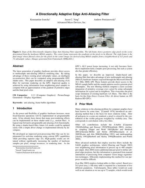
Figure 1: Steps of the Directionally Adaptive Edge Anti-Aliasing Filter algorithm. The left frame shows geometry edge pixels in the scene
determined from the hardware MSAA samples. The center frame represents the gradients at the pixels to be filtered. The right frame is the
final image where filtered colors for the pixels in the center image are derived using MSAA samples from a neighborhood of 3x3 pixels and
72 subsample values. (Images generated from Futuremark 3DMark03.)
Abstract
The latest generation of graphics hardware provides direct access
to multisample anti-aliasing (MSAA) rendering data. By taking
advantage of these existing pixel subsample values, an intelligent
reconstruction filter can be computed using programmable GPU
shader units. This paper describes an adaptive anti-aliasing (AA)
filter for real-time rendering on the GPU. Improved quality is
achieved by using information from neighboring pixel samples to
compute both an approximation of the gradient of primitive edges
and the final pixel color.
CR Categories: I.3.3 [Computer Graphics]: Picture/Image
Generation—Display Algorithms;
Keywords: anti-aliasing, frame buffer algorithms
1 Introduction
As the power and flexibility of graphics hardware increases, more
fixed-function operations will be implemented on programmable
units. It has already been shown that many post-rendering effects
can be implemented on these shader units (e.g., motion blur). A
logical step forward is programable anti-aliasing (AA) functionally.
By using a shader-based filter, future AA modes could be updated
easily with a simple driver change or implemented directly by developers.
We developed an improved post-processing filter that can be implemented
for real-time rendering using current GPU capabilities
while providing superior edge AA. High-quality results are obtained
without significantly increasing the number of hardware
samples per pixel, storage resources, or rendering time. As the
∗ Konstantine.Iourcha@amd.com
† JasonC.Yang@amd.com
‡ Andrew.Pomianowski@amd.com
GPU’s ALU power keeps increasing, it not only becomes feasible
to implement fairly complex post-processing, but such a system
also has greater efficiency.
In this paper, we describe an improved, shader-based antialiasing
filter that takes advantage of new multisample anti-aliasing
(MSAA) hardware features exposed through the Microsoft DirectX
10.1 [Mic 2008] API. These features provide direct access to the
MSAA sample buffer and the sample patterns used to generate pixel
subsamples. The new filtering method computes a more accurate
integration of primitive coverage over a pixel by using subsample
information for a pixel and its neighbors. This overcomes the pixel
scope limitation of existing hardware AA filters. This filter is the
basis for the Edge-Detect Custom Filter AA driver feature on ATI
Radeon HD GPUs.
2 Prior Work
Many solutions to the aliasing problem for computer graphics have
been known for some time. [Catmull 1978] introduced an antialiasing
method that is the basis for most solutions today. After
all polygons in a scene are rendered, a pixel is colored by the contribution
of the visible polygons weighted by visibility area. This
corresponds to convolution with a box filter.
Other AA contributions include the A-buffer [Carpenter
1984][Schilling and Strasser 1993][Wittenbrink 2001], stochastic
sampling [Dippé and Wold 1985][Keller and Heidrich
2001][Akenine-Möller and Ström 2003][Hasselgren et al.
2005][Laine and Aila 2006][Schilling 1991], and multisampling
[Akeley 1993][Haeberli and Akeley 1990][Beaudoin and Poulin
2004].
More advanced methods that employ non-box filters include the
SAGE graphics architecture, which [Deering and Naegle 2002]
uses neighboring pixel information to process up to 400 samples
per output. [Sen 2004] stores additional data per pixel to define subpixel
edge positions, but this information is generated from manual
annotations of processing from computer vision image segmentation
techniques. Efficiently implementing this method for our purposes
would be difficult.
[Lau Mar 2003] employs lookup tables to filter a pixel. Based on a
5x5 pixel area, a 1M entry table is required for a maximum of five
different gradations. Unfortunately, these tables would not scale
well in our situation as we use up to 72 samples, which would result

Figure 2: The left pixel shows the area contribution by a primitive.
In MSAA, the coverage area is approximated using the sub-pixel
samples. On the right, the pixel is considered 3/4 covered.
in a 1G+ entry table. Furthermore, we explicitly try to avoid table
usage to avoid consuming GPU memory and bandwidth as well as
irregular memory access patterns.
[Rokita 2005] and [Rokita 2006] are extremely simple and inexpensive
approaches to AA and would generate too few levels of
intensity gradations. Adapting this approach to our requirements
would be difficult.
There are relevant works in the adjacent fields of image and
video upsampling [Li and Orchard Oct 2001][Zhang and Wu 2006]
[Su and Willis 2004][Wang and Ward 2007][Asuni and Giachetti
2008][Giachetti and Asuni 2008][Yu et al. 2001], but most of
those algorithms would be difficult to adapt for our purposes.
The straightforward application of these algorithms to our problem
would be to upscale multisampled images about twice and
then integrate samples on the original pixels, but this would require
computing 16 to 24 additional samples per-pixel, which has a prohibitively
high computational cost. Also, these algorithms are designed
around upsampling on Cartesian grids and their adaptation
to non-uniform grids (used in hardware multisampling based AA)
is not always obvious. Finally, some upsampling methods may not
completely avoid edge blurring in the cross direction, which we try
to eliminate as much possible.
Our method is closer to those based on isolines such as [Wang and
Ward 2007], but we use a much simpler model as no actual upsampling
happens (we do not need to calculate new samples; in fact
we downsample), nor do we need to process all pixels (we can use
a standard resolve for the pixels which do not fit our model well).
Moreover, we avoid explicit isoline parameter computation other
than the local direction. This allows us to perform the processing
in real-time using a small fraction of hardware recourses while still
rendering the main application at the same time.
3 Hardware Anti-Aliasing
The two most popular approaches to anti-aliasing on the graphics
hardware are supersampling and MSAA.
Supersampling is performed by rendering the scene at a higher resolution
and then downsampling to the target resolution. Supersampling
is expensive in terms of both performance and memory bandwidth.
However, the results tend to have high quality, since the
entire scene is rendered at a higher resolution. Downsampling is
performed by a resolve, which is the aggregation of the samples
with filtering.
MSAA is an approximation to supersampling and is the predominant
method of anti-aliasing for real-time graphics on GPUs (Figure
2). Whenever a pixel is partially covered by a polygon, the single
color contribution of the polygon to the pixel at subsample locations
Figure 3: Isolines running through the center pixel with samples
used for the function value. Segments inside the pixel are the
weights used for integration.
is stored in the MSAA buffer along with the coverage mask [Akeley
1993]. When the scene is ready for display, a resolve is performed.
In most implementations, a simple box filter is used that averages
the subsample information.
Hardware MSAA modes are characterized by the pattern of the
sampling grid. Most graphics hardware employ a non-uniform grid.
We take advantage of the existing hardware by using as input the
data stored in the MSAA buffers after rendering. We then replace
the standard hardware box-filter with a more intelligent resolve implemented
using shaders.
4 Directionally Adaptive Edge AA Filter
Our primary goals are to improve anti-alised edge appearance and
the pixel coverage estimation when using MSAA on primitive
edges with high contrast (Figure 2). In this section we first introduce
the filtering method by using a basic single channel example.
Then we present the full algorithm details.
4.1 Single Channel Case
For simplicity, consider a single channel continuous image (we can
use R,G, or B channels or a luma channel of the original image),
which can be viewed as a function. To produce an output value for
a pixel we need to integrate this function over the pixel area. The
standard approximation is to take multiple samples (more or less
uniformly distributed) and average them.
If we know isolines of the function, we can use a sample anywhere
on the isoline (possibly outside of the pixel area) to determine the
function value. Therefore, we can take a set of isoline segments
inside the pixel (more or less uniformly distributed) for which we
have the sample function values and calculate their weighted average
(with the weights being the lengths of the isoline segments
inscribed by the pixel) to produce the final pixel value (Figure 3).
This allows for a more accurate pixel value estimate for the same
sample density, as samples outside of the pixel can be used to estimate
function values on the isolines, however, we need to calculate
the isolines.
If the curvature of the isolines is locally low, we can model them
with straight lines. To derive these lines we can compute a tangent

plane in the center of the pixel and use it as a linear approximation
of the function (assuming it is sufficiently smooth). The gradient
of this plane is collinear with the gradient of the function and will
define the direction of isoline tangents (and approximating straight
isolines).
We can extend this model to a discrete world. Having a number
of discrete samples (possibly on a non-uniform grid) we can find a
linear approximation of the function using a least squares method
and use its gradient and isolines as an approximation. Note, if the
error of approximation is relatively small, this generally means that
the original function is “close to linear” in the neighborhood, the
curvature of its isolines can be ignored, and our model works. If,
on the other hand, the error is large, this would mean that the model
is not valid, and we fall back to a standard sample integration for
that pixel (as we generally use a very conservative approach in our
algorithm) without creating any artifacts.
The actual images are, however, a three-channel signal, so we need
to generalize the above for this case. One way would be to process
each channel, but this would considerably increase processing
time and may create addition problems when gradients in different
channels have vastly different directions. The other possibility, often
employed for similar purposes [Yu et al. 2001] is to use only
the luminance for isoline determination. However, this would miss
edges in chrominance, which is undesirable. Our solution is to follow
the framework above and to fit a vector valued linear function
of the form described in details below. With that in mind we will
still use the terms “gradient approximation” and “isoline approximation”
below.
4.2 Algorithm Overview
When processing, we are only interested in pixels that are partially
covered by primitives. We can determine this by inspecting the
MSAA subsamples of a pixel (Section 3). If there are differing
subsample color values, we will further process the pixel.
We are not interested in pixels that are fully covered by a primitive
(all subsamples having the same values); those pixels are processed
as usual (i.e., a box filter). Fully covered (interior) pixels are usually
textured and we ignore texture edges because they are pre-filtered
or processed by other means.
For pixels that are partially covered, we are mainly interested in
those in the middle of long edges (those that extend across several
pixels), where jaggies are most visible. Assuming that the isolines
and edges do not have high curvature at the pixel, then the three
channel signal f(v) ∈ R 3 at the point v = [x, y] can be approximated
in the neighborhood of the pixel as
f(v) ≈ ˜ f(〈g, v〉) (1)
where ˜ f : R 1 → R 3 is a function of a scalar argument into color
space and g, v ∈ R 2 is the gradient approximation and the point
position [x, y] respectively. 〈 , 〉 represents a dot product.
Gradient Calculation We want to find an approximation (1)
where ˜ f is a linear function which minimizes the squared error:
F = X
(C1 · 〈g, vi〉 + C0) − f(vi) 2
i∈I
where I is the set of samples in the neighborhood of interest (in our
case 3x3 pixels), C1, C0 ∈ R 3 are some constant colors (RGB),
and f(vi) are the color samples. We find an approximation to the
(2)
Figure 4: Integration Model. 1) Construct a square around the
pixel, with two sides orthoganal to g (⊥g) . 2) Extend the rectangle,
in the direction ⊥g until it meets the 3x3 pixel boundary. 3) For
every sample vi, the line segment, from the line passing through the
sample and ⊥g, enscribed by the pixel is the weight wi. 4) Using
eq. (5) the pixel color is calculated.
gradient by minimizing F over C0, C1, and g using standard least
squares techniques [Korn and Korn 1961].
The resulting minimization problem can be solved as follows: First,
if vi are centered such that P
i∈I
vi = 0 (this can be achieved with
an approapriate substitution) then C0 is the mean of {f(vi)}i∈I,
hence we can assume without loss of generality that {vi}i∈I and
{f(vi)}i∈I are both centered. Differentiating on components of
C1 results in a linear system which can be analytically solved. Substituting
this solution for C1 into (2) transforms it into a problem
of maximizing the ratio of two non-negative quadratic forms. This
is essentially 2x2 eigenvector problems and can be easily solved.
Note, that we do not compute C1 numerically at all, (as all we need
is g).
If the solution for g is not unique this means that either C1 is zero
(the function is approximated by a constant) or different image
channels (components of f) do not correlate at all (i.e., there is no
common edge direction among the channels). In either case we ignore
the pixel. If performance is a concern, the computations can be
simplified by using aggregate samples per pixel instead of the original
vi. For many applications this provides sufficient accuracy. On
the other hand, if detection of a particular image feature is needed
with higher accuracy, other (possibly non-linear) ˜ f can be used, but
usually at a much higher computational cost.
Although the accuracy of our integration is dependent on the accuracy
of the gradient approximation, we found that errors resulting
from error in the gradient estimates are not significant.
Thresholding Of concern are regions with edges of high curvature
(i.e., corners) or having non-directional high frequency signal

where unique solutions of the above least squares problem still exist.
Since we assume isolines are locally straight or have low curvature,
filtering hard corners with our integration method may cause
undesired blurring.
To reduce potential blurring from these cases, we can reject pixels
from further processing by using the following thresholding
δ(vi) = f(vi) − (C1 · 〈g, vi〉 + C0) (3)
P
i∈I δ(vi)2
P
i∈I f(vi) − C02
! 1/2
≤ threshold (4)
The pixel passes if eq. (4) holds using a threshold that is relatively
small. This would imply that the approximation of eq. (1) is valid.
We can also control the amount of blurring by adjusting the threshold.
Note, that if we have an estimate of g in (2), we can use it with ˜ f
of a different form. So, we could find an optimal step-function ˜ f
approximation (2) using the obtained g and use it for more precise
thresholding. However, the computational cost would be too high
for real-time processing and we found that the method provides satisfactory
results without it.
Generally, the filtering requirements are application dependent;
some professional applications (for instance flight simulators) are
required to have a minimal amount of high frequency spacial and
temporal noise while bluring is not considered a significant problem.
The situation is often opposite in game applications where big
amount of high frequency noise can be tolerated (and even at some
times this is confused with “sharpness”), but blury images are not
appreciated.
Therefore, no “universal threshold” can be specified, but we found
that a threshold appropriate for an application can be easily found
experimentally; an implementation could have a user adjustable
slider.
Stochastic Integration Under assumption (1), the following integration
can be used. A gradient-aligned rectangle, which approximately
aligns with isolines, is constructed by taking a circumscribed
square around the pixel with two sides orthogonal to g and
extruding it in the direction orthogonal to g until it meets with the
boundary of the 3x3 pixel area centered at the pixel (Figure 4).
Now consider all the sample positions vi within the resulting rectangle.
To calculate the weight wi of a sample vi, under the assumption
of (1), we take a line passing through the sample orthogonal to
g (s.t. 〈g, v〉 = 〈g, vi〉). The computed weight wi is equal to the
length of the segment of this line enclosed by the pixel. The total
result for the pixel is then
P
i∈I R f(vi) · wi
P
i∈I R wi
where IR is the set of indices for the samples inside the rectangle.
Increasing the number of samples, provided they are uniformly distributed,
can give a better integral approximation. However, the
rectangle cannot be increased too far because the edge in the actual
scene might not extend that far out. Visually, in our experiments,
the weighting as described works well and provides good performance
and quality. Alternatively, the weights could be decreased
(5)
O
X
X
X
X
X
O
O
O
X
X
X
O
X
X
O
X
X
X
O
O
Figure 5: Example pattern masks used to eliminate potential problem
pixels. X’s represent edges and O’s represent non-edges. Empty
grid spaces can be either edge or non-edge. The edge pixel (at center)
would be eliminated from processing if its neighbors do not
match one of the patterns.
for samples further from the pixel, but this would reduce the number
of color gradations along the edge.
Masking Earlier, we used thresholding from (4) to eliminate potential
problem pixels. We can further eliminate pixels by looking
at edge patterns within an image. In our implementation, this occurs
before finding the gradient.
A 3x3 grid pattern of edge and non-edge pixels, centered around the
candidate pixel, is matched against desired patterns. For example,
if only a center pixel is marked as an edge, the pixel is most likely
not a part of a long primitive edge and we exclude it from processing.
If all pixels in the 3x3 region are marked as edge pixels, we
conservatively assume that no dominating single edge exists and
fall-back to standard processing as well. Figure 5 shows a subset of
the pattern masks used to classify edges for processing. Defining
a complete classifier is a non-obvious task (see discussion in [Lau
Mar 2003]).
Any pixels that have been rejected during the entire process (thresholding
and masking) are resolved using the standard box filter resolve.
In our experiments, we found that pixels evaluated with our
method neighboring those of the standard resolve produced consistent
color gradients along edges.
5 Results
5.1 Implementation and Performance
In our implementation, we use four, full-screen shader passes corresponding
to each part of the filtering algorithm (see Figure 1 for
a subset):
Pass 1 Identify edge pixels using the MSAA buffer. Seed the
frame buffer by performing a standard resolve at each pixel.
Pass 2 Mask out candidate pixels using edge patterns.
Pass 3 Compute the edge gradient for pixels that were not rejected
in the last pass and use thresholding to further eliminate
pixels. Values are written to a floating point buffer.
Pass 4 Derive the final frame buffer color for the pixels from
the previous pass through stochastic integration using samples
from a 3x3 pixel neighborhood. Integration and weights are

calculated in the shader. All other pixels have already been
filtered during the first pass.
Shaders were developed using DirectX HLSL Pixel Shader 4.1. All
parts of the algorithm are computed in shader with no external tables.
Weights and masks are computed dynamically. Pixels that are
rejected from subsequent passes can be identified by either writing
to a depth buffer or a single channel buffer along with branching in
the shader.
We tested the performance of our shader implementation using
8xAA samples on an ATI Radeon HD 4890 running on several
scenes from Futuremark 3DMark03. Rendering time for the filter
was between 0.25 to 1.7 ms at 800x600 resolution, 0.5 to 3 ms
at 1024x768, and 1 to 5 ms at 1280x1024. Each pass refines the
number of pixels that need processing, therefore rendering time is
dependent on the number of edges in a frame. See Figure 7 for
example scenes.
Currently there is some memory overhead due to the multi-pass implementation,
but since only a small percentage of pixels in a frame
are actually being processed, performance could be improved by using
general compute APIs such as OpenCL. Our algorithm should
scale with the number of shader processors, so future hardware improvements
and features would also improve the rendering time.
Also, the number of passes was chosen mostly for performance and
could be combined on future hardware.
5.2 Quality
Figure 6 compares the results of the new adaptive AA filter against
existing hardware AA methods on a near horizontal edge for a scene
rendered at 800x600 resolution. As a comparison, we also rendered
the scene at 2048x1536 with 8x AA and downsampled to 800x600
to approximate rendering with supersampling. Our new filter, using
existing hardware 4xAA samples, can produce a maximum of 12
levels of gradation. By using existing hardware 8x AA samples,
the filter can achieve up to 24 levels of gradation.
Figure 7 compares the new AA filter against the standard box filter
over various scenes and at different resolutions. The important
characteristics to note in the image are the number of color graduations
along the edges and their overall smoothness. Simultaneously
it can also be observed that there is no blurring in the direction perpendicular
to each edge when compared to methods that use narrow
band-pass filters with wider kernels. Effectively, our filter is as
good as a standard hardware resolve with 2 to 3 times the number of
samples. We also do not observe temporal artifacts with our filter.
The differences between our filter and current hardware AA methods
can be perceived as subtle, but our goal was to only improve the
quality of edges. These differences are on the same order of magnitude
as the differences between 8x and 16x AA or higher. Full
screen image enhancement, although a possible future line of work,
is outside the scope of this paper.
One drawback with our method is the aliasing of thin objects such
as wire, grass blades, etc. There are cases where the given sampling
density within a pixel is not capable of reproducing the object, but
the object is detected in neighboring pixels and potentially resulting
in gaps in the on-screen object rendering. Although it is possible
to try to detect and correct these gaps to a point (i.e., through the
masking step), the better solution is higher sampling resolution.
6 Future Work and Conclusions
There are several avenues for future research. Better but costlier
edge detection algorithms could be used to find pixels amenable to
processing. This includes other edge patterns for the refinement of
potential edge pixels. Instead of using the existing MSAA samples
and coverage masks, our algorithm could be applied to supersampling
as well as filtering pixels with edges in textures. It might be
possible to improve results by designing a better subsample grid.
Finally, it might be possible to adapt our method to image upsampling.
We have presented an improved anti-aliasing filter compared to current
hardware methods using new hardware features exposed using
DirectX 10.1. Our filter is another example of rendering improvements
using increased programmability in hardware. Improved
anti-aliasing is an obvious use for the new MSAA features and we
expect future developers to find more interesting applications.
Acknowledgements
The authors would like to thank to Jeff Golds for help in the implementation.
References
AKELEY, K. 1993. Reality engine graphics. In SIGGRAPH ’93:
Proceedings of the 20th annual conference on Computer graphics
and interactive techniques, ACM, New York, NY, USA, 109–
116.
AKENINE-MÖLLER, T., AND STRÖM, J. 2003. Graphics for the
masses: a hardware rasterization architecture for mobile phones.
ACM Trans. Graph. 22, 3, 801–808.
ASUNI, N., AND GIACHETTI, A. 2008. Accuracy improvements
and artifacts removal in edge based image interpolation. In VIS-
APP (1), 58–65.
BEAUDOIN, P., AND POULIN, P. 2004. Compressed multisampling
for efficient hardware edge antialiasing. In GI ’04:
Proceedings of Graphics Interface 2004, Canadian Human-
Computer Communications Society, 169–176.
CARPENTER, L. 1984. The A-buffer, an antialiased hidden surface
method. In SIGGRAPH ’84: Proceedings of the 11th annual
conference on Computer graphics and interactive techniques,
ACM Press, New York, NY, USA, 103–108.
CATMULL, E. 1978. A hidden-surface algorithm with anti-aliasing.
In SIGGRAPH ’78: Proceedings of the 5th annual conference on
Computer graphics and interactive techniques, ACM Press, New
York, NY, USA, 6–11.
DEERING, M., AND NAEGLE, D. 2002. The sage graphics architecture.
In SIGGRAPH ’02: Proceedings of the 29th annual conference
on Computer graphics and interactive techniques, ACM
Press, New York, NY, USA, 683–692.
DIPPÉ, M. A. Z., AND WOLD, E. H. 1985. Antialiasing through
stochastic sampling. In SIGGRAPH ’85: Proceedings of the 12th
annual conference on Computer graphics and interactive techniques,
ACM Press, New York, NY, USA, 69–78.
GIACHETTI, A., AND ASUNI, N. 2008. Fast artifacts-free image
interpolation. In British Machine Vision Conference.
HAEBERLI, P., AND AKELEY, K. 1990. The accumulation buffer:
hardware support for high-quality rendering. In SIGGRAPH ’90:
Proceedings of the 17th annual conference on Computer graphics
and interactive techniques, ACM, New York, NY, USA, 309–
318.

(a) No AA
(b) 4xAA
(c) 8xAA
(d) 16xAA
(e) New filter using 4xAA samples
(f) New filter using 8xAA samples
(g) Downsampled from high resolution rendering
Figure 6: A comparison of different AA methods applied to a pinwheel from FSAA Tester by ToMMTi-Systems (top) rendered at 800x600.
Shown is a subset of the scene where the edges are at near horizontal angles. (e) shows the new filter using hardware 4xAA samples. In this
example, 10 levels of gradation is visually achieved. (f) is the new filter using 8xAA samples. In this example 22 levels of gradation is visually
achieved. (d) is Nvidia’s 16Q AA filtering. (g) is a downsample of the original scene rendered at 2048x1536 and 8x AA.

(a) (b) NoAA (c) 4xAA (d) New 4xAA (e) 8xAA (f) New 8xAA
Figure 7: Comparison of the various AA filters applied on various scenes and at different resolutions. Column (b) is no AA enabled. (c)
and (e) are the standard AA resolve at 4x and 8x samples respectively. (d) and (f) are results from the new filtering using the existing 4x and
8x MSAA samples respectively. The first and second rows (Futuremark 3DMark03) are rendered at 800x600 resolution and the third row
(Futuremark 3DMark06) is rendered at 1024x768.
HASSELGREN, J., AKENINE-MÖLLER, T., AND HASSELGREN,
J. 2005. A family of inexpensive sampling schemes. Computer
Graphics Forum 24, 4, 843–848.
KELLER, A., AND HEIDRICH, W. 2001. Interleaved sampling. In
Proceedings of the 12th Eurographics Workshop on Rendering
Techniques, Springer-Verlag, London, UK, 269–276.
KORN, G., AND KORN, T. 1961. Mathematical Handbook for
Scientists and Engineers. McGraw-Hill, Inc.
LAINE, S., AND AILA, T. 2006. A weighted error metric and optimization
method for antialiasing patterns. Computer Graphics
Forum 25, 1, 83–94.
LAU, R. Mar 2003. An efficient low-cost antialiasing method based
on adaptive postfiltering. Circuits and Systems for Video Technology,
IEEE Transactions on 13, 3, 247–256.
LI, X., AND ORCHARD, M. Oct 2001. New edge-directed interpolation.
IEEE Transactions on Image Processing 10, 10, 1521–
1527.
MICROSOFT CORPORATION. 2008. DirectX Software Development
Kit, March 2008 ed.
MYSZKOWSKI, K., ROKITA, P., AND TAWARA, T. 2000.
Perception-based fast rendering and antialiasing of walkthrough
sequences. IEEE Transactions on Visualization and Computer
Graphics 6, 4, 360–379.
ROKITA, P. 2005. Depth-based selective antialiasing. Journal of
Graphics Tools 10, 3, 19–26.
ROKITA, P. 2006. Real-time antialiasing using adaptive directional
filtering. In Real-Time Image Processing 2006. Proceedings of
the SPIE., vol. 6063, 83–89.
SCHILLING, A., AND STRASSER, W. 1993. Exact: algorithm
and hardware architecture for an improved a-buffer. In SIG-
GRAPH ’93: Proceedings of the 20th annual conference on
Computer graphics and interactive techniques, ACM, New York,
NY, USA, 85–91.
SCHILLING, A. 1991. A new simple and efficient antialiasing
with subpixel masks. In SIGGRAPH ’91: Proceedings of the
18th annual conference on Computer graphics and interactive
techniques, ACM Press, New York, NY, USA, 133–141.
SEN, P. 2004. Silhouette maps for improved texture magnification.
In HWWS ’04: Proceedings of the ACM SIG-
GRAPH/EUROGRAPHICS conference on Graphics hardware,
ACM, New York, NY, USA, 65–73.
SU, D., AND WILLIS, P. 2004. Image interpolation by pixel-level
data-dependent triangulation. Computer Graphics Forum 23, 2,
189–201.
WANG, Q., AND WARD, R. 2007. A new orientation-adaptive
interpolation method. Image Processing, IEEE Transactions on
16, 4 (April), 889–900.
WITTENBRINK, C. M. 2001. R-buffer: a pointerless a-buffer hardware
architecture. In HWWS ’01: Proceedings of the ACM SIG-
GRAPH/EUROGRAPHICS workshop on Graphics hardware,
ACM, New York, NY, USA, 73–80.
YU, X., MORSE, B. S., AND SEDERBERG, T. W. 2001. Image reconstruction
using data-dependent triangulation. IEEE Comput.
Graph. Appl. 21, 3, 62–68.
ZHANG, L., AND WU, X. 2006. An edge-guided image interpolation
algorithm via directional filtering and data fusion. Image
Processing, IEEE Transactions on 15, 8 (Aug.), 2226–2238.