SQUIDs - Low Temperature Laboratory
SQUIDs - Low Temperature Laboratory
SQUIDs - Low Temperature Laboratory

Create successful ePaper yourself
Turn your PDF publications into a flip-book with our unique Google optimized e-Paper software.
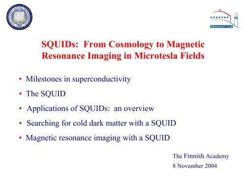
<strong>SQUIDs</strong>: From Cosmology to Magnetic<br />
Resonance Imaging in Microtesla Fields<br />
• Milestones in superconductivity<br />
• The SQUID<br />
• Applications of <strong>SQUIDs</strong>: an overview<br />
• Searching for cold dark matter with a SQUID<br />
• Magnetic resonance imaging with a SQUID<br />
The Finnish Academy<br />
8 November 2004
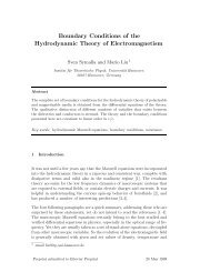
Centigrade/Kelvin/Fahrenheit <strong>Temperature</strong> Scales<br />
Room temperature<br />
Ice point<br />
Vostok, Antarctica -88 o C<br />
8/24/60<br />
B.P. liquid nitrogen 77K<br />
B.P. liquid helium 4.2K<br />
o C<br />
0<br />
-100<br />
-200<br />
-273<br />
K<br />
273<br />
173<br />
73<br />
0<br />
Absolute zero<br />
o F<br />
32<br />
-459
Milestones in Superconductivity<br />
1911 Kamerlingh Onnes discovers zero resistance
Heike Kamerlingh Onnes<br />
Courtesy Kamerlingh Onnes <strong>Laboratory</strong>, University of Leiden
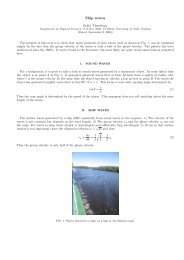
The Discovery of Superconductivity<br />
Resistance (Ω)<br />
4.0 4.2<br />
<strong>Temperature</strong> (K)<br />
4.4<br />
Resistance vanishes below the transition (or critical) temperature T c
Magnetic Fields<br />
The earth Bar magnet<br />
~1 gauss<br />
10 -4 tesla<br />
~1000 gauss<br />
0.1 tesla
Zero Resistance<br />
Magnetic field<br />
• Current persists forever<br />
I<br />
• Resistance at least one billion billion<br />
times less than copper<br />
• Basis of superconducting magnets
A Few Other Superconductors<br />
Element T c<br />
Aluminum 1.2 K<br />
Indium 3.4 K<br />
Tin 3.7 K<br />
Lead 7.2 K<br />
Niobium 9.2 K<br />
• “Type I” superconductors<br />
• Driven normal by magnetic<br />
fields less than 2000 gauss
Milestones in Superconductivity<br />
1911 Kamerlingh Onnes discovers zero resistance<br />
1957 Bardeen, Cooper and Schrieffer develop “BCS” theory
Normal Metals vs. Superconductors<br />
Normal Metals Superconductors : BCS Theory<br />
Electron has charge -e<br />
I I<br />
Scattering of electrons produces resistance.<br />
A current generates a voltage, and hence<br />
causes dissipation.<br />
Electrons are paired together :<br />
these Cooper pairs have charges -2e<br />
I I<br />
Cooper pairs carry a supercurrent which<br />
encounters no resistance.<br />
A supercurrent generates no voltage, and<br />
hence causes no dissipation.
Milestones in Superconductivity<br />
1911 Kamerlingh Onnes discovers zero resistance<br />
1957 Bardeen, Cooper and Schrieffer develop “BCS” theory<br />
1957 Alexei Abrikosov predicts Type II superconductors Large-scale applications<br />
are made possible
Alloys: ~2000 known<br />
Type II Superconductors<br />
The secret of their success: Type II materials admit “vortices” of<br />
magnetic field, and the supercurrents flow around them.<br />
High field magnets made possible.
Flux Quantization<br />
Φ = n Φ 0<br />
J<br />
Φ = nΦ 0 (n = 0, ±1, ±2, ...)<br />
where<br />
Φ 0 ≡ h/2e ≈ 2 x 10 -15 Wb<br />
is the flux quantum
Milestones in Superconductivity<br />
1911 Kamerlingh Onnes discovers zero resistance<br />
1957 Bardeen, Cooper and Schrieffer develop “BCS” theory<br />
1957 Alexei Abrikosov predicts Type II superconductors<br />
1960 Ivar Giaever invents tunnel junctions<br />
1962 Brian Josephson invents “Josephson Tunneling”<br />
Large-scale applications<br />
are made possible<br />
Superconducting<br />
electronics is born
• Cooper pairs tunnel through barrier<br />
I<br />
I<br />
I<br />
Nb film<br />
Josephson Tunneling<br />
oxidized Nb film<br />
V<br />
insulating<br />
barrier<br />
superconductor superconductor<br />
V<br />
~ 20 Å<br />
Current<br />
Created the field of superconducting electronics<br />
Brian Josephson 1962<br />
I<br />
Voltage
Milestones in Superconductivity<br />
1911 Kamerlingh Onnes discovers zero resistance<br />
1957 Bardeen, Cooper and Schrieffer develop “BCS” theory<br />
1957 Alexei Abrikosov predicts Type II superconductors<br />
1960 Ivar Giaever invents tunnel junctions<br />
1962 Brian Josephson invents “Josephson Tunneling”<br />
1986 Bednorz and Muller discover high-T c superconductivity<br />
Large-scale applications<br />
are made possible<br />
Superconducting<br />
electronics is born
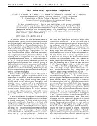
<strong>Temperature</strong> (Kelvin)<br />
Transition <strong>Temperature</strong> Over the Years<br />
160<br />
120<br />
80<br />
40<br />
Nb NbN<br />
Bi 2Sr 2Ca 2Cu 3O 10<br />
(La/Sr)CuO 4<br />
HgBa 2Ca 2Cu 3O 8<br />
YBa 2Cu 3O 7<br />
Hg<br />
(1911)<br />
0<br />
Pb<br />
Nb3Ge SrTiO3 1910 1960 1980<br />
Year<br />
2000<br />
MgB 2<br />
-100 °C<br />
liquid N 2<br />
liquid He
YBCO
Milestones in Superconductivity<br />
1911 Kamerlingh Onnes discovers zero resistance<br />
Nobel Prize 1913<br />
1957 Bardeen, Cooper and Schrieffer develop “BCS” theory<br />
Nobel Prize 1972<br />
1957 Alexei Abrikosov predicts Type II superconductors<br />
Nobel Prize 2003<br />
1960 Ivar Giaever invents tunnel junctions<br />
Nobel Prize 1973<br />
1962 Brian Josephson invents “Josephson Tunneling”<br />
Nobel Prize 1973<br />
1986 Bednorz and Muller discover high-T c superconductivity<br />
Nobel Prize 1987<br />
Large-scale applications<br />
are made possible<br />
Superconducting<br />
electronics is born
The SQUID
The dc Superconducting Quantum Interference Device<br />
• dc SQUID<br />
Ib<br />
Two Josephson junctions on a superconducting ring<br />
I<br />
• Current-voltage (I-V) characteristic modulated by magnetic flux Φ:<br />
Period one flux quantum Φ o = h/2e = 2 x 10 -15 T m 2<br />
I<br />
nΦ o<br />
(n+1/2)Φ o<br />
∆V<br />
V<br />
δV<br />
V<br />
δΦ<br />
V<br />
0 1 2<br />
Φ<br />
Φo
20 µm<br />
Josephson junctions<br />
<strong>Low</strong>-T c SQUID<br />
Operating temperature = 4.2 K<br />
Multilayer device: niobium - aluminum oxide - niobium<br />
500 µm<br />
Nb-AlOx-Nb SQUID<br />
with input coil
B N ~ 1 fT Hz -1/2<br />
Superconducting Flux Transformer:<br />
Magnetometer and Gradiometer<br />
Flux-locked<br />
SQUID<br />
Flux-locked<br />
SQUID
Magnetic Fields<br />
1 femtotesla<br />
tesla<br />
10 -4<br />
10 -6<br />
10 -8<br />
10 -10<br />
10 -12<br />
10 -14<br />
10 -16<br />
Earth’s field<br />
Urban noise<br />
Car at 50 m<br />
Human heart<br />
Fetal heart<br />
Human brain response<br />
SQUID
Applications of <strong>SQUIDs</strong>:<br />
An Overview
Olli Lounasmaa<br />
Olli was did much to bring <strong>SQUIDs</strong> to Finland, and greatly<br />
encouraged their application to Magnetoencephalography (MEG).<br />
MEG is the single biggest consumer of <strong>SQUIDs</strong>, and<br />
has important applications in both brain research and clinical<br />
diagnosis. Neuromag is a leading supplier of MEG systems around<br />
the world. Olli was also deeply involved with the use of <strong>SQUIDs</strong> to<br />
study nuclear ordering in copper and silver at ultralow<br />
temperatures.
Neuromag ® 306-Channel SQUID System<br />
for Magnetoencephalography
Applications of Magnetoencephalography<br />
Clinical (Reimbursable in the United States)<br />
• Presurgical screening of brain tumors (evoked response)<br />
• Location of epileptic foci (spontaneous signals)<br />
Research<br />
• Language mapping in the brain<br />
• Identification of patients with schizophrenia<br />
• Identification of patients with dyslexia<br />
• Alzheimer's disease<br />
• Parkinson's disease<br />
• Neurological recovery following stroke or hemorrhage
CardioMag Imaging System for<br />
Magnetocardiography
Quantum Design "Evercool"
2G Superconducting Rock Magnetometer
SQUID Surveying for Minerals<br />
Courtesy Cathey Foley (CSIRO)
MAGMA-C1 Scanning SQUID Microscope<br />
Neocera, Inc.
Atacama Pathfinder EXperiment
Courtesy Stanford<br />
University and NASA<br />
Gravity Probe-B<br />
Tests of General Relativity
UC Berkeley Flux Qubits<br />
Qubit 2<br />
Qubit 1<br />
35 µm
Searching for Axions: The Microstrip SQUID Amplifier<br />
University of Gießen<br />
Michael Mück<br />
Jost Gail<br />
Christoph Heiden †<br />
UCB, LBNL and LLNL<br />
Marc-Olivier André<br />
Darin Kinion<br />
Jan Kycia<br />
Support: DOE/BES<br />
DOE/HEP<br />
NSF
Cold Dark Matter<br />
• Recent cosmic microwave background measurements indicate that<br />
~25% of the mass of the universe is cold dark matter (CDM).<br />
• A candidate particle is the axion, proposed in 1978 to explain the<br />
absence of a measurable neutron electric dipole moment.<br />
• The axion is predicted to be a very light particle with no charge or spin.
Resonant Conversion of Axions into Photons<br />
Pierre Sikivie (1983)<br />
Primakoff Conversion Expected Signal<br />
Power<br />
∆ν<br />
~ 10<br />
ν<br />
−6<br />
Frequency
Axion Detector at<br />
Lawrence Livermore<br />
National <strong>Laboratory</strong>
Noise <strong>Temperature</strong><br />
R<br />
T<br />
-A<br />
[ T + T ( R)<br />
]R<br />
0<br />
2<br />
SV (f) = A ⋅4k<br />
B N<br />
V 0
LLNL Axion Detector<br />
• Current system noise temperature: T S = T + T N ≈ 3.2 K<br />
Cavity temperature: T ≈ 1.5 K<br />
Amplifier noise temperature: T N ≈ 1.7 K<br />
• Time to scan the range of frequencies from f 1 to f 2 :<br />
τ(f 1 ,f 2 ) ≈ 4 x 10 16 (T S /1 K) 2 (1/f 1 –1/f 2 ) sec<br />
For f 1 = 0.24 GHz, f 2 = 2.4 GHz: τ ≈45 years<br />
• Note: There is only a factor of 2 to be gained in T S by reducing T<br />
unless T N is also reduced.
Microstrip SQUID Amplifier<br />
Conventional SQUID Amplifier Microstrip SQUID Amplifier<br />
• Source connected to both ends of coil • Source connected to one end of the<br />
coil and SQUID washer; the other end<br />
of the coil is left open
Gain (dB)<br />
30<br />
25<br />
20<br />
15<br />
10<br />
Gain vs. Coil Length<br />
100<br />
71 mm<br />
200<br />
νres ν (MHz)<br />
res (MHz)<br />
600<br />
400<br />
200<br />
33 mm<br />
300 400 500<br />
Frequency (MHz)<br />
20 40 60<br />
Coil Length (mm)<br />
15 mm<br />
600<br />
7 mm<br />
700
Noise <strong>Temperature</strong> of Microstrip Amplifier<br />
At 20 mK the noise temperature is 50mK, about 40 times lower<br />
than that of the current semiconductor amplifier
Microstrip SQUID Amplifier: Impact on Axion Detector<br />
• Current LLNL axion detector: T S ≈ 3.2 K<br />
• For T ≈ T N ≈ 50 mK: T S ≈ T + T N ≈ 100 mK<br />
τ≈45 years x (0.1/3.2) 2<br />
≈ 18 days
Summary<br />
• Gain ≥ 20 dB for frequencies ≤ 1 GHz<br />
• Cooled to 20 mK, T N is within a factor of 2 of the quantum limit<br />
• Noise temperature 40 times lower than state-of-the-art cooled semiconductor<br />
amplifiers<br />
Future directions<br />
• Implement second-generation axion detector: expected to increase scan<br />
rate by three orders of magnitude<br />
• Post-amplifier for radio-frequency single-electron transistor: should<br />
enable quantum-limited charge amplifier
Microtesla Nuclear Magnetic Resonance and Magnetic<br />
Resonance Imaging<br />
• Nuclear magnetic resonance<br />
• Magnetic resonance imaging<br />
Michael Hatridge<br />
Nathan Kelso<br />
SeungKyun Lee<br />
Robert McDermott<br />
Michael Mössle<br />
Michael Mück<br />
Whit Myers<br />
Bennie ten Haken<br />
Andreas Trabesinger<br />
Erwin Hahn<br />
Alex Pines
Energy<br />
z<br />
B 0<br />
Nuclear Magnetic Resonance<br />
Protons<br />
M<br />
B 0<br />
E = +µ p B<br />
ν 0 = 42.58 MHz/tesla<br />
ω0 = γB0 E = -µ pB Magnetic moment (µpB0
High Field MRI<br />
3T MRI scanner (GE) 1.5T MRI scanner (GE)
Timeline<br />
Michael Crichton, 1999<br />
“Most people”, Gordon said, “don’t realize that the<br />
ordinary hospital MRI works by changing the quantum<br />
state of atoms in your body ... But the ordinary MRI does<br />
this with a very powerful magnetic field - say 1.5 tesla,<br />
about twenty-five thousand times as strong as the earth’s<br />
magnetic field. We don’t need that. We use<br />
Superconducting QUantum Interference Devices, or<br />
<strong>SQUIDs</strong>, that are so sensitive they can measure resonance<br />
just from the earth’s magnetic field. We don’t have any<br />
magnets in there”.
The “Cube”
Three dimensional images of pepper<br />
1 2<br />
3<br />
1 2<br />
3<br />
20 mm<br />
4<br />
5 6<br />
4 5<br />
6<br />
1 6
T 1 -weighted Contrast Imaging<br />
• T 1 is the relaxation time of the proton spins<br />
• T 1 depends strongly on the environment of the protons<br />
• T1-weighted contrast imaging is widely used in conventional MRI<br />
T<br />
to distinguish different types of tissue<br />
• T 1 (malignant tissue) > T 1 (normal tissue)<br />
• T 1-contrast can be much higher in low fields
B = 13.2 mT<br />
int<br />
T 1 contrast images of<br />
agarose gel<br />
0.25%<br />
0.5%<br />
agarose<br />
B = 300 mT<br />
int
Forearm (20 mm slice)<br />
B p ~ 40 mT<br />
B 0 = 132 µT<br />
B 0 = 4 T<br />
4T image:<br />
Courtesy of Ben Inglis,<br />
Henry H. Wheeler, Jr.<br />
Brain Imaging Center,<br />
UC Berkeley
Future directions for low-field MRI<br />
• Reduce system noise<br />
• Increased signal-to-noise ratio<br />
• Reduced acquisition time<br />
• Multichannel system<br />
• Increased signal-to-noise ratio<br />
• Improved spatial resolution<br />
• Increased coverage<br />
• Combine low-field MRI with existing technology<br />
for magnetoencephalography (MEG)<br />
• <strong>Low</strong>-cost “open” MRI system<br />
• Screening for tumors (with T 1-weighted contrast)<br />
• Imaging knee, foot, elbow, wrist ...<br />
• Monitoring T1 in bone marrow