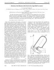
pdf-file - Institut für Theoretische Physik

Boundary Conditions of the
Hydrodynamic Theory of Electromagnetism
Abstract
Sven Symalla and Mario Liu 1
Institut für Theoretische Physik, Universität Hannover,
30167 Hannover, Germany
The complete set of boundary conditions for the hydrodynamic theory of polarizable
and magnetizable media is obtained from the differential equations of the theory.
The qualitative distinction of different numbers of variables that exists between
the dielectrics and conductors is stressed. The theory and the boundary conditions
presented here are covariant to linear order in v/c.
Key words: hydrodynamic Maxwell equations, boundary conditions, covariance
1 Introduction
It was not until a few years ago that the Maxwell equations were incorporated
into the hydrodynamic theory in a rigorous and consistent way, complete with
dissipative terms and valid also in the nonlinear regime [1]. The resultant
theory accounts for the low frequency dynamics of macroscopic systems that
are exposed to external fields, or contain electric charges and currents. It was
helpful in understanding the curious spin-up behavior of ferrofluids [2], and
has produced a number of interesting predictions [3,4].
The four following paragraphs are a quick summary, addressing those who are
surprised by these statements, yet do not intend to read the references [1–4]:
The macroscopic Maxwell equations certainly belong to the best studied and
verified differential equations in physics, especially in the optical range of frequency.
Yet they are usually taken as a set of stand-alone equations, decoupled
from other macroscopic variables. So the evolution of the electromagnetic field
is generally obtained with given and set values of density, temperature and
1 email liu@itp.uni-hannover.de
Preprint submitted to Elsevier Preprint 28 May 1998

local velocity, among others. In a few notable exceptions, these parameters are
taken as functions of time. A rigorous and trustworthy theory, on the other
hand, needs to consider these macroscopic, hydrodynamic quantities also as
variables, and include their dynamics with that of the field. For instance, given
the continuity equation for the momentum and its modification through the
presence of electromagnetic field, we will find an unambiguous answer to the
notoriously difficult question of what is the ponderomotive force for a nonstationary,
dissipative system of nonlinear constitutive relations [2,3]. This is
a typical feed-back effect of how fields influence the hydrodynamic variables.
And it is simply neglected if the velocity is given as a parameter, even if a
function of time.
Starting from the thermodynamic approach to electromagnetism as given in
the justifiably famous Vol 8 of Landau and Lifshitz [5], a theory that accounts
for the dynamics of both the field and the hydrodynamic variables simultaneously
is essentially what has been achieved in [1–4]. Most of the papers are
confined to the true hydrodynamic regime of local equilibrium, though a first
attempt of generalizing to the dispersive, optical frequency range has proven
rather successful [3].
One striking result of this theory is the appearance of dissipative fields, H D
and E D that are gradients of the original fields. They account for dissipative
phenomena such as the restoration of equilibrium – even if the constitutive
relations are nonlinear. (In contrast, the identification of the imaginary parts
of ε and µ with dissipation holds only for strictly linear constitutive relations.)
Despite the k-dependence, or the appearance of spatial dispersion, H D and E D
include temporal dispersion. (In fact, even in the linear case, these dissipative
fields are more general that the accounts of temporal dispersion. The difference
is large in select systems, especially dielectric ferrofluids [4].)
The higher order gradient terms in the dissipative fields necessitate additional
boundary conditions for the Maxwell equations, although no additional variables
are being considered. This is the principle difference to the many works
on the subject of “Additional Boundary Conditions”, where either higher frequency
dynamic variables such as the exitonic degrees of freedom, or low
frequency, surface variables are being considered [6].
One of the main foundations of this new, hydrodynamic theory of electromagnetism
is a pragmatic combination of the Galilean and the Lorentz transformation
to first order in v/c: The former is employed for all hydrodynamic
variables, including the temporal and spatial derivative, and the latter used for
the field variables. As a result, the equations of motion are not covariant. This
is cause for worry, because although the difference between the Galilean and
the first-order Lorentz transformation is known to be irrelevant in usual hydrodynamic
theories, circumstances are not as clear-cut when electromagnetic
2

fields are involved.
This is the reason a fully relativistic version of the same theory was derived [7],
employing only the Lorentz transformation, and demonstrating unambiguously
the consistency of the hydrodynamic theory of electromagnetism. While
this is clearly the correct theory to apply for relativistic systems such as quickly
spinning astrophysical objects, it falls short when used to decide whether the
original theory is indeed the appropriate and rigorously valid one for nonrelativistic
systems. For this purpose, one needs to go one step further, derive
the complete set of boundary conditions, and thoroughly check whether any
term not contained in the original theory could conceivably be important. The
first part of this work is the content of the present paper.
The hydrodynamic theory and the boundary conditions, covariant to first
order in v/c, are presented here. We distinguish clearly between dielectrics and
conductors, because the theory for conductors has less independent variables,
and hence also less boundary conditions. And because the transition between
the two theories is subtle and prone to errors.
The boundary conditions are derived from the bulk equations themselves,
with the help of irreversible thermodynamics. This deviates from the strictly
mathematical concept of differential equations, where boundary conditions
are extrinsic information, used to select a special solution out of the manifold
satisfying the equation.
The most well known example of the approach in physics is the derivation
of boundary conditions from the Maxwell equations, yielding results such as
the continuity of the normal component of the magnetic field B [5]. And
there are many more recent examples: Boundary conditions have been derived
especially for broken symmetry systems, (such as liquid crystals [8], superfluid
4 He [9] and 3 He[10], including the A→B transition [11],) but also for the more
mundane shear flows of isotropic liquids [12].
The boundary conditions to be derived below are being applied to understand
the viscosity of ferrofluids, and to dynamo theory. These results will be presented
elsewhere. (In fact, one or two of the more unconventional boundary
conditions have already been used [2,4], though without proper derivation or
presentation.)
The paper has four more chapters, the first two to present the hydrodynamic
theory, for dielectrics and conductors, respectively, and the third to set up
the boundary conditions. A fourth chapter considers two specific situations to
clarify the physics contained in some of the boundary conditions.
3

2 The Hydrodynamic Theory for Dielectrics
2.1 Lorentz Transformation and Thermodynamics
The starting point of every hydrodynamic theory is the thermodynamic theory.
The energy density ɛ tot is a function of all the other conserved quantities, the
entropy density s and the field variables B and D. For a two-component liquid
we have, in the rest frame,
dɛ tot =dε + c 2 dρ = T ds +(µ + c 2 )dρ
+µc dρc + H · dB + E · dD , (1)
where the constraints
∇·B =0, ∇·D = ρel (2)
are satisfied in equilibrium. (ρel is the charge density.) Note that ɛ tot is the total
energy including the rest mass. The mass densities, ρ and ρc, are connected
to the particle numbers n1 and n2 by
ρ = m1 n1 + m2 n2 , ρc = m2 n2, (3)
where m1 and m2 denote the respective masses. The choice of µ + c 2 as the
conjugate variable to ρ renders the expansion in the small parameter ε/ρ c 2
simple. (At most densities, the rest mass is certainly the by far dominating
contribution.)
The equilibrium fluxes of energy and momentum in the rest frame are [5],
Q = c E × H , (4)
Πij =(Ts+ µρ+ µc ρc + E · D + H · B − ε) δij
− 1
2 [Hi Bj + Ei Dj +(i ↔ j))] . (5)
These variables and their fluxes constitute the energy-momentum 4-tensor
Π µν ,
Π 00 = ɛ tot , Π 0k =Π k0 = Qk/c = cg tot
k ,
Π ik =Πik =Πki . (6)
The local conservation laws ensure that Π µν satisfies
4

∂νΠ µν = 0 (7)
and is symmetric. (The greek indices go from 0 to 3, the latin ones from 1 to
3.)
The Lorentz transformation will now yield these thermodynamic expressions
for an arbitrary inertial frame. Denoting the rest frame quantities with the
superscript 0 , the Lorentz transformation
Π µν =Λ µ
α
Π αβ 0
Λ ν
β , (8)
for v = v ex employs with the matrix
where
Λ ν
⎛
⎞
⎜ γ γβ 00⎟
⎜
⎟
⎜
⎟
⎜ γβ γ 00⎟
µ = ⎜
⎟
⎜
⎟ ,
⎜ 0 0 1 0 ⎟
⎝
⎠
(9)
0 0 0 1
β = v/c , γ =1/ 1 − β2 . (10)
Up to order v2
c 2 ,wehave
ɛ tot =(1+v 2 /c 2 )ɛ tot,0
+2 v [1 + v 2 /c 2 ] · g tot,0
+vi Π 0 ij vj/c 2 , (11)
cg tot
i = Qi/c = vi/c (1 + v 2 /c 2 ) ɛ tot,0
+[1 + v 2 /(2 c 2 )] cg tot,0
i
+3 vi cg tot,0
l vl/(2 c 2 )
+[1 + v 2 /(2 c 2 )] vl Π 0 li/c
+vi vl (Π 0 lk/c) vk/(2 c 2 ), (12)
Πik = vi vk ɛ tot,0 /c 2 +[1+v 2 /(2 c 2 )] vi g tot,0
k
+[1 + v 2 /(2 c 2 )] vk g tot,0
i
+ vi vk g tot,0
l
vl/(vc 2 )
+Π 0 ik +Π 0 il vl vk/(2 c 2 )
+Π 0 lk vl vi/(2 c 2 ) . (13)
As ε ≪ ρc2 , we shall only include terms of linear order in v,
except for terms
c
connected to the rest mass, ρc2 , where quadratic order will be included. (In the
5

energy flux, this leads to a third order term.) Then the lab-frame expressions
for the energy, momentum and the fluxes are
where
g tot =(Ts+ µρ+ µc ρc + ρc 2 ) v/c 2 + E × H/c , (14)
Q = c 2 g tot + vl gl v , (15)
Πij =(Ts+ µρ+ µc ρc + v · g
+E · D + H · B − ε) δij
+ 1
2 [gi vj − Ei Dj − Hi Bj +(i ↔ j))] , (16)
g = g tot − D × B/c . (17)
The other thermodynamic variables also need to be transformed. First, the
four fields:
B 0 = B − v × E/c , D 0 = D + v × H/c , (18)
H 0 = H − v × D/c , E 0 = E + v × B/c . (19)
Both chemical potentials, µ + c 2 and µc, obey analogous formulas:
µ + c 2 =[1− v 2 /(2 c 2 )] (µ 0 + c 2 ) , (20)
µc =[1− v 2 /(2 c 2 )] µ 0 c . (21)
However, because of c 2 , only µ is altered
µ = µ 0 − v 2 /2 , (22)
while µc = µ 0 c remains invariant in linear order of v.
The quantities s, ρc
c
and T are also invariant to this order, s = s0 , ρc = ρ0 c and T = T 0 .Inthe
combination ρc2 ,wehave
ρ =[1+v 2 /(2 c 2 )] ρ 0 ; (23)
otherwise, it is ρ = ρ 0 .
Because ε ≪ ρc 2 , the nonrelativistic expression for g tot is
g tot = ρ v + E × H/c . (24)
6

Putting all this together, the Π 00 -component yields
dε =dɛ tot − c 2 dρ = T ds + µ dρ + µc dρc + v · dg
+H · dB + E · dD . (25)
The isotropy of the system, ie the invariance of the energy density under an
infinitesimal rotation implies:
v × g + H × B + E × D =0. (26)
2.2 The Equilibrium Conditions
Maximizing the integrated entropy d 3 rs under the constrains of various
conservation laws and Eqs(2), the resulting Euler-Lagrange equations, or the
equilibrium conditions are [7]
where
∂tT =0, ∂tµ =0, ∂tµc =0,
∂tH 0 =0, ∂tE 0 =0, vij =0,
∇µ + ∂tv + µ∂tv/c 2 =0,
∇ 0 T − 1
µ + c2 T ∇0 µ =0,
∇ 0 µc − 1
µ + c2 µc ∇ 0 µ =0,
∇ 0 × H 0 + 1
µ + c2 H0 ×∇ 0 µ =0,
∇ 0 × E 0 + 1
µ + c2 E0 ×∇ 0 µ = 0 (27)
∇ 0 = ∇ + v
c 2 ∂t , vij = 1
2 (∇ivj + ∇jvi) . (28)
Note the preponderance of rest frame quantities. Except for the chemical potential,
all spatial derivatives are small. If the charges are eventually able to
move around, the total entropy may be further maximized if
E 0 =0. (29)
7

2.3 The Hydrodynamic Equations
In local equilibrium, the conditions of Eqs(27) are not met, and the left hand
sides (that we shall call thermodynamic forces) are not zero. This leads to
dissipative terms (denoted below by the superscript D ) and entropy production
as functions of the thermodynamic forces, which parameterize the deviation
from global equilibrium. The variables of course still obey continuity equations,
with
0=∂t(B + B D )+c ∇×(E + E D ) ,
0=∂t(D + D
(30)
D )+j D el +(ρel + ρ D el) v
−c ∇×(H + H D ) , (31)
0=∂t(ρ + ρ D )+∇·(ρ v − j D ) , (32)
0=∂t(ρc + ρ D c )+∇·(ρc v − j D c ) , (33)
R/T = ∂t(s + s D )+∇·(s v − f D ) , (34)
0=∂t (g tot
i + g tot,D
i )+∇j (Πij − Π D ij) , (35)
0=∂t(ɛ tot + ε D )+∇·(Q + Q D ) (36)
∇·(B + B D )=0, (37)
∇·(D + D D )=ρel + ρ D el . (38)
We may subtract the equation of motion for mass from that of the total energy
ɛ tot , to arrive at the continuity equation for the non-relativistic form of energy
conservation, more usual in hydrodynamic theories,
0=∂t(ε + ε D − ρ D c 2 )+∇·(Q + Q D
−ρc 2 v + c 2 j D ) . (39)
The covariance of the Eqs(30 - 38) has a number of consequences:
• The equilibrium contributions of energy, momentum and their fluxes constitute
the equilibrium energy-momentum 4-tensor Π µν ; the same applies
to the nonequilibrium contributions, ε D , Q D , g tot,D and −Π D ij constitute the
nonequilibrium 4-tensor Π D,µν .
• Analogously, all fields, the equilibrium and nonequilibrium ones, (E, B),
(E D , B D ), (D, H) and (D D , H D ) constitute 4-tensors of the form
8

(E, B) µν ⎛
⎞
⎜ 0 −Ex −Ey −Ez ⎟
⎜
⎟
⎜
⎟
⎜ Ex 0 −Bz By ⎟
= ⎜
⎟
⎜
⎟ .
⎜ Ey Bz 0 −Bx
⎟
⎝
⎠
(40)
Ez −By Bx 0
• The equilibrium quantities (s, s v/c), (ρ, ρ v/c), (ρc,ρc v/c) and (ρel c, ρel v)
are 4-vectors. The same applies to the nonequilibrium quantities (s D c, −f D ),
(ρ D c, −j D ), (ρ D c c, −j D c ) and (ρ D el c, j D el).
The dissipative contributions of the variables s D , ρ D , ρ D c , g tot,D , B D , D D and
ρ D el vanish in the local rest frame, v = 0, because this is where the nonrelativistic
and relativistic physics overlap. Here, according to the concept of local
equilibrium, the variables only contain equilibrium information. As a result,
their form in an arbitrary frame is given as:
B D = v × E D /c , D D = −v × H D /c , (41)
ρ D el = v · j D el/c 2 , s D = −v · f D /c 2 , (42)
ρ D = −v · j D /c 2 , ρ D c = −v · j D c /c 2 , (43)
g tot,D
i = −Π D ij vj/c 2 , (44)
and because of the symmetry of the energy-momentum 4-tensor,
with
yet an order higher.
Q D i = c 2 g tot,D
i = −vj Π D ij, (45)
ε D = O
v 2 /c 2
(46)
To actually obtain the dissipative currents, we substitute ∂tɛ tot in Eq(36) for
the expressions of Eq(25),
T∂ts +(µ + c 2 ) ∂tρ + µc ∂tρc + v · ∂tg + H · ∂tB
+E · ∂tD + ∂tε D = −∇ · (Q + Q D ) , (47)
insert the appropriate equations of motion, Eqs(30 - 35), excluding terms of
order higher than v
c , and arrive at two expressions, the energy flux QD i and
the entropy production R. The energy flux is
9

Q D i = −(µ + c 2 ) j D i − µc j D c,i − Tf D i
+c
E D × H 0 + E 0 × H D
i − vj Π D ij , (48)
which in conjunction with Eq(45) leads to
(µ + c 2 ) j D i = −µc j D c,i − Tf D i
+c
E D × H 0 + E 0 × H D
. (49)
i
(It is now plain that jD i ∼ c−2 is relativistically small, and it is well justified
to ignore it in non-relativistic theories.)
The entropy production is
R = f D ·∇ 0 T +Π D ij vij + j D c ·∇ 0 µc + j D ·∇ 0 µ + j D el E 0
+E D · c
∇ 0 × H 0
− H D · c
∇ 0 × E 0
. (50)
Inserting Eq (49), the number of independent thermodynamic forces is reduced
by one,
R = f D
· ∇ 0 T − 1
µ + c2 T ∇0
µ +Π D ij vij
+j D
c · ∇ 0 µc − 1
µ + c2 µc ∇ 0
µ + j D el E 0
+E D
· c ∇ 0 × H 0 + 1
µ + c2 H0 ×∇ 0
µ
−H D
· c ∇ 0 × E 0 + 1
µ + c2 E0 ×∇ 0
µ . (51)
It is instructive to compare this equation with Eq(27). Clearly, the thermodynamic
forces there appear here again. If they vanish, we have equilibrium,
and the entropy production R is zero. If they do not, the leading terms in R,
being a positive definite function, must be quadratic in these forces. In this
order, the dissipative currents, f D ,Π D ij, j D c , E D , H D , j D el, are proportional to
the forces, with the coefficients obeying the Onsager symmetry relations.
3 The Hydrodynamic Theory for Conductors
If the electrical conductivity is large enough, such that the displacement current
∂tD in
10

0= ˙ D + j D el + ρel v − c ∇×(H + H D ) (52)
is negligible with respect to j D el = σ E 0 , it may then be eliminated. This is the
quasi-stationary approximation[5], always justified in the low-frequency limit:
Consider (for v ≡ 0)
| ˙ D|≈ωεE ≪ j D = σE, (53)
(where ε is the dielectric constant,) and find
ω ε/σ ≪ 1. (54)
We shall in this work refer to a system as a conductor if the quasi-stationary
approximation is valid. (If not, the displacement current ∂tD needs to be
included and, despite some residual conductivity, the equations of the last
section apply.)
In the Heaviside-Lorentz system of units, the conductivity of metals is of the
order of σ =10 18 /s, eight to ten orders of magnitude above the frequencies
at which local equilibrium reigns and the hydrodynamic theory is valid. So
the quasi-stationary approximations always apply in these systems, which can
therefore be considered as conductors without any qualification. If the conductivity
is below 10 10 /s, circumstances are more complicated and depend on
the given frequency.
The elimination of the displacement current ∂tD is a qualitatively important
step, as this is equivalent to the statement that D is no longer an independent
variable of the hydrodynamic theory. Indeed, the relaxation time of the electric
field is τ = ε
σ ,as
| ˙ E|≈E/τ ≈ ˙ D/ε ≈ σ E/ε . (55)
and the electric field has ample time to relax for frequencies ωτ ≪ 1. So,
taking E 0 as zero in equilibrium, the rest frame thermodynamics is now,
dɛ tot = T ds +(µ + c 2 )dρ + µc dρc + H · dB . (56)
Note that the electric field need not vanish in the lab-frame, v = 0, though of
course only via the Lorentz transformation
E = −v × B/c , D = −v × H/c , (57)
11

without changing the fact that they are not independent. Note also that we
have only implemented the fact that the equilibrium electric field vanishes.
Off equilibrium, it does not, and as we know may drive a current through a
wire. It remains dependent, however, and is in this case given by
c ∇×(H + H D )=σE. (58)
There are two ways to arrive at the hydrodynamic theory for conductors, one
may either set to zero all terms ∼ D 0 and E 0 in the previous theory, or one
may start from scratch with a reduced set of variables. Both methods lead to
the same results, which are presented below.
The basic thermodynamic identity for an arbitrary inertial system is,
where
dε =dɛ tot − c 2 dρ = T ds + µ dρ + µc dρc
+v · dg tot + H · dB (59)
g tot =(Ts+ µρ+ µc ρc + ρc 2 ) v
1 v
− × B × H
c2 c c
≈ ρ v − 1
v
× B × H . (60)
c c
In equilibrium, the magnetic field satisfies
∇·B =0. (61)
To linear order in v,
the fields
c
H 0 = H , B 0 = B (62)
are Lorentz invariant.
The change in the equilibrium conditions are in the Euler-Lagrange equations
for the field. Only
∂tH =0, ∇ 0 × H + 1
µ + c 2 H ×∇0 µ =0, (63)
remain, with E 0 ≡ 0 implied. The rotational identity Eq(26) reduces to
H × B =0. (64)
12

The hydrodynamic equations are
with
0=∂t(B + B D )+c ∇×(−v × B/c + E D ) , (65)
0=∂t(ρ + ρ D )+∇·(ρ v − j D ) , (66)
0=∂t(ρc + ρ D c )+∇·(ρc v − j D c ) , (67)
R
T = ∂t(s + s D )+∇·(s v − f D ) , (68)
0=∂t (g tot
i + g tot,D
i )+∇j (Πij − Π D ij) ,
0=∂t(ε + ε
(69)
D − ρ D c 2 )
+∇·(Q + Q D − ρc 2 v + j D ) (70)
0=∇·(B + B D ) , B D = v × E D /c , (71)
Q =(Ts+ µρ+ µc ρc + ρc 2 + v · g) v
− (v × B) × H , (72)
g = g tot +(v × H) × B/c 2 = ρ v , (73)
Πij =[Ts+ µρ+ µc ρc + v · g + H · B − ε] δij
+ 1
2 [gi vj − Hi Bj +(i ↔ j))] , (74)
(µ + c 2 ) j D i = −T f D i − µc j D c,i + c
E D × H
, (75)
i
R = f D
· ∇ 0 T − 1
µ + c2 T ∇0
µ +Π D ij vij
+j D
c · ∇ 0 µc − 1
µ + c2 µc ∇ 0
µ
+E D
· c ∇ 0 × H + 1
µ + c2 H ×∇0
µ . (76)
The quantities s D , ρ D , ρ D c , Q D i , g tot,D , ε D satisfy the same relations as before,
see Eq(42 - 46). The dissipative fluxes are again obtained in an expansion of
the entropy production R, Eq(76).
The two Maxwell equations (31, 38) are not part of the hydrodynamic theory;
rather, they simply define the quantities ρel and j D el,
j D el + ρel v := c ∇×H + ∂t (v × H) /c ,
ρ + ρ D el := −∇ · (v × H) /c . (77)
Note that H D ∼∇×E 0 has been set to zero, while ρ D is given by Eq(42).
13

4 Boundary Conditions
A solution of the hydrodynamic equations is possible only if in addition to the
equations we also have the appropriate initial and boundary conditions. The
latter are obtained from the bulk equations themselves. Therefore, number
and type of the boundary conditions depend on the two systems comprising
the interface. The boundary conditions are best derived in the rest frame of the
interface, (or more generally in the rest frame of the portion of the interface
under consideration).
4.1 The Dielectric-Dielectric Interface, without Phase Transition
We shall first consider the simpler case in which no mass current may cross
the interface, ie in the absence of the possibility of a phase transition, such as
given at an interface made from two different substances.
The first boundary condition is the continuity of the normal component of the
energy flux,
∆(Qn + Q D n )=0, (78)
where the subscript n denotes the component normal to the interface. This
condition is obtained by integrating the energy conservation,
˙ɛ tot + ∇·(Q + Q D )=0,
over an infinitesimally thick slab around the stationary interface. Physically, it
simply implies that the same amount of energy enters and leaves the interface.
The notation, here and below, is given as
∆A ≡ A(r − rsf →−0)
−A(r − rsf → +0) ≡ A1 − A2 , (79)
A ≡〈A〉 ≡ 1
2 (A1 + A2) , (80)
where rsf is a given point on the surface. The normal vector n hence points
into region 2. Also,
∆(AB) ≡ A1 B1 − A2 B2 = A ∆B + B ∆A. (81)
All vectors are divided into an tangential and a normal component, say
14

vt = v − (v · n) n , (82)
vn =(v · n) n . (83)
The lack of mass transfer implies
ρ1 v1,n = j D 1,n , ρc,1 v1,n = j D c,1,n ,
ρ2 v2,n = j D 2,n , ρc,2 v2,n = j D c,2,n . (84)
Because j D 1,n and j D 2,n are relativistically small quantities, so are v1,n and v2,n,
hence also j D c,1,n and j D c,2,n.
Three more boundary conditions follow from the conservation of momentum,
one per component. In comparison to the conservation of energy, however,
there is a complication arising from the possibility of an isotropic surface
pressure[13],
Π tot
ij ≡ Πij − Π D ij − αsf (δij − ninj) δ(|r − rsf|), (85)
where αsf is the surface energy density of [13]. After some algebra, we obtain
where
∆(Πnn − Π D
1
nn) =αsf
R1
+ 1
,
R2
(86)
∆(Πt,i − Π D t,i) t1,i = −t1 ·∇αsf , (87)
∆(Πt,i − Π D t,i) t2,i = −t2 ·∇αsf
Πt,i =Πlj nj (δil − ni nl) ,
(88)
Π D t,i =Π D lj nj (δil − ni nl) , (89)
R1, R2 denote the curvature radii, and t1, t2 the attendant principle directions.
The radii are positive if they point into region 1, and the bulge is toward region
2.
From the Maxwell equations, we deduce the boundary conditions,
∆(Bn + B D n )=0, (90)
∆(Et + E D t )=0, (91)
∆(Dn + D D n )=−σsf , (92)
∆(Ht + H D t )=n × jel,sf/c , (93)
15

where σsf denotes the surface charge density and jel,sf the surface current, as
yet undetermined.
Combining Eqs(78) and (84), we obtain
0=∆(Qn + Q D n +(µ + c 2 ) j D n − (µ + c 2 ) ρvn) . (94)
which in conjunction with Eqs(49, 15, 45) implies
0=∆
(T s+ v · g) vn − Π D nj vj − Tf D n
+c
E × H + E D × H 0 + E 0 × H D
· n
. (95)
If the interface is curved, we shall from here on choose the inertial system
vt = 0 (which gets rid of a term ∼ vtαsf in R sf ), otherwise, vt is arbitrary.
As vn is negligibly small in the absence of phase transition, Eq(95) is quickly
converted into the surface entropy production,
R sf ≡−T ∆fn = fn ∆T − Π D jn ∆vt,j
+c ∆
E × H + E D × H 0 + E 0 × H D
· n (96)
with fn ≡ (svn − f D n ), here and below. The surface entropy production R sf ≡
−T ∆fn is the difference between the entropy current exiting and entering the
surface. Just as its bulk counter part, it is positive definite, invariant under
time inversion and vanishes in equilibrium. Some more algebra then yields
R sf = fn ∆T + c
n × E D
· ∆H + c
H D × n
· ∆E
+(−Π D jn + H D j Bn + E D j Dn + 1
4 σsf∆Ej)∆vt,j
+[n × jel,sf] · (n × E 0 ) , (97)
a nice sum of independent pairs of force and fluxes. Taking them to be proportional
to each other, they represent another seven boundary conditions, and
determine the surface current jel,sf.
One symmetry element peculiar to the interface is the invariance of R sf under
the simultaneous operation n → −n and ∆ → −∆. Taking this and the
isotropy into account, we find
⎛
fn = κs∆T
⎞ ⎛
(98)
⎜ n × ED ⎟ ⎜
⎝ ⎠ = ⎝
n × jel,sf
βs
⎞ ⎛
γs ⎟ ⎜ c ∆Ht
⎠ ⎝
¯γs σs n × E0 ⎞
⎟
⎠ , (99)
16

⎛
⎜
⎝ −ΠD,eff t,i
HD × n
⎞ ⎛
⎟ ⎜
⎠ = ⎝
i
ηs
⎞ ⎛
ζs ⎟ ⎜
⎠ ⎝
¯ζs αs
∆vt,i
⎞
⎟
⎠
c ∆Et,i
(100)
where −Π D,eff
t,i
≡−Π D t,i + H D t,i Bn + E D t,i Dn + 1
4 σsf∆Et,j, and
¯γs = −γs , ¯ ζs = −ζs . (101)
αs,βs,ηs,κs,σs > 0 . (102)
These are altogether 21 boundary conditions. They suffice to determine (i) all
(outgoing) hydrodynamic modes of the dielectric medium, 9 for each side; (ii)
the normal components of B + B D and D + D D , (iii) the lab velocity. See [14]
for a more detailed consideration (in single-component liquids).
4.2 The Dielectric-Dielectric Interface, with Phase Transition
Mass and concentration currents across the interface renders the consideration
slightly more complicated.
The 12 continuity conditions remain:
∆(Qn + Q D n )=0, (103)
∆(ρvn − j D n )=0, (104)
∆(ρc vn − j D c,n) = 0 (105)
∆(Πnn − Π D nn) =Psf , (106)
∆(Πt,i − Π D t,i) t1,i = t1 ·∇αsf , (107)
∆(Πt,i − Π D t,i) t2,i = t2 ·∇αsf
(108)
∆(B D n + Bn) =0, (109)
∆(Et + E D t )=0, (110)
∆(D D n + Dn) =−σsf , (111)
∆(Ht + H D t )=n × jel,sf/c . (112)
The rest of 9 boundary conditions must now be deduced from R sf . Combining
Eq(103) and (104), we obtain
0=∆(Qn + Q D n ) − (µ + c 2 )∆(ρvn − j D n )
=∆(Qn + Q D n +(µ + c 2 ) j D n − (µ + c 2 ) ρvn)
+〈ρvn − j D n 〉∆µ, (113)
17

which in conjunction with Eqs(49, 15, 45) leads to
0=∆
(T s+ µc ρc + v · g) vn − Π D nj vj − Tf D n
−µc j D c,n + c
E × H + E D × H 0
+E 0 × H D
· n
+ 〈ρvn − j D n 〉∆µ. (114)
Employing Eq(105), we have
R sf = −T ∆fn = fn ∆T + 〈ρvn − j D n 〉∆µ
+〈ρc vn − j D c,n〉∆µc − ∆(vj Π D jn)
+∆ (v · g vn)+c ∆
E × H + E D × H 0
+E 0 × H D
· n, (115)
which is more suitably written as
where
R sf = fn ∆T + 〈ρc vn − j D c,n〉∆µc
+
〈vn gj〉−Π D jn + 1
4 σsf∆Ej
∆vt,j
+〈ρvn − j D n 〉 ∆µ eff
+c n ×〈E D − vn
× B〉 · ∆H
c 0
+c 〈H D + vn
× D〉×n · ∆E
c 0
+[n × jel,sf] · (n × E 0 ) , (116)
µ eff
≡ µ +
v2 n gn
(ρvn − jD n ) − ΠDnn vn
(ρvn − jD
. (117)
n )
This R sf yields 9 boundary conditions and the value of the surface current
jel,sf.
4.3 Interfaces involving Conductors
The essential difference to the boundary conditions considered until now is
the fact that the electric field D is no longer an independent variable. As a
direct result, neither are the two boundary conditions,
18

∆(D D n + Dn) =−σsf , (118)
∆(Ht + H D t )=n × jel,sf/c. (119)
This also affects the surface entropy production. Starting from
0=∆(Qn + Q D n ) − (µ + c 2 )∆(ρvn − j D n )
=∆(Qn + Q D n +(µ + c 2 ) j D n − (µ + c 2 ) ρvn)
+〈ρvn − j D n 〉∆µ (120)
we have for the conductor-conductor interface
0=∆
(T s+ µc ρc + v · g) vn − Π D nj vj
−T f D n − µc j D c,n + c
E × H + E D × H
· n
and hence
or
+〈ρvn − j D n 〉∆µ, (121)
R sf = −T ∆fn = fn ∆T + 〈ρvn − j D n 〉∆µ
+〈ρc vn − j D c,n〉∆µc − ∆(vj Π D jn)+∆(v · g vn)
+c ∆
E × H + E D × H
· n (122)
R sf = fn ∆T + 〈ρc vn − j D c,n〉∆µc
+
〈vn gj〉−Π D
jn ∆vt,j
+〈ρvn − j D n 〉 ∆µ eff
+c
n ×
E D + E
· ∆Ht , (123)
where µ eff is the same as before, see Eq(117). This expression yields 7 connecting
conditions. So we have a total of 16 boundary conditions for the conductorconductor
interface. They suffice to determine all outgoing collective modes,
7 for each side, the normal component of B + B D , and the lab velocity of
the interface. (Note that the number of the collective modes is reduced in a
conductor, because there are no sq-Modes [4]. Also, the electromagnetic waves
are reduced to magnetic, diffusive modes.)
For the conductor-dielectric interface, Eq(120) implies
0=∆
(T s+ µc ρc + v · g) vn − Π D nj vj − Tf D n
19

−µc j D c,n + c
E × H + E D × H 0
+〈ρvn − j D n 〉∆µ − c
E 0 2 × H D 2
· n
· n , (124)
where 2 denotes the dielectric, ie n points into the dielectric. The entropy
production is now
R sf = fn ∆T + 〈ρc vn − j D c,n〉∆µc
+
〈vn gj〉−Π D
jn ∆vt,j
+〈ρvn − j D n 〉 ∆µ eff
+
n ×
E D + E
· c ∆H 0 t
+
H D
2 + v2/c × D2 · c
E 0 2 × n
. (125)
This Rsf yields 9 boundary conditions. Ignoring cross terms, we have especially
n ×
E D + E
= βsc ∆H 0 t, βs > 0 . (126)
Here we have altogether 18 boundary conditions. They suffice to determine
the 7 collective modes of the conductor and the 9 collective modes of the
dielectric, to fix the normal component of B + B D and to determine the lab
velocity of the interface.
5 Two Illustrative Examples
The hydrodynamics is not simply a coarse-grained theory; it has a scaleinvariance
built in: Varying the resolution, the hydrodynamics remains valid.
This feature makes the theory especially general and widely applicable. The
same applies to the boundary conditions derived above, which are valid where
ever the bulk theory is. Below are two examples for the vacuum-conductor
interface, where we shall calculate some coefficients from two simple models.
In both cases, we shall employ a higher resolution hydrodynamic theory to
obtain the coefficient of the coarser-grained one.
More specifically, we shall in the first example calculate the coefficient in the
boundary condition Eq(126), and understand the discontinuity of the coarsegrained
magnetic field H as given by a highly conducting surface layer (and
surface current) that is not explicitly accounted for in the given resolution.
This is of course a trivial case, but it does serve to draw one scenario in which
the discontinuity of the magnetic field is not surprising. The crucial point
here is that the coarse-grained boundary conditions as presented above are
applicable also for situations where a higher resolution theory is not easily
20

available, such as for a turbulent boundary layer. If we check our ambitions
with respect to resolving the turbulence in details, this layer and its turbulence
enhanced magnetic diffusivity should be well accounted for by the same
boundary condition.
The second example is less straight forward. Here, we employ the hydrodynamic
theory for a dielectric as the higher resolution description of the conductor.
This sounds somewhat surprising at first and should be explained.
The dielectric theory (including a finite conductivity) contains a stationary,
collective mode (the sq-mode) that is given by an exponential decay of the
electromagnetic field from the system’s surface [4]. Because the decay length
shrinks with the conductivity, the hydrodynamic theory for conductors does
not contain this mode, (though this may be amended by including higher order
gradient terms). Nevertheless, the derived boundary conditions are such
that the long ranged effects of the sq-mode are well accounted for, albeit on
a grain size on which the sq-mode is no longer resolved. This statement is
explicitly proven by comparing the dielectric with the conductor theory.
5.1 The Highly Conducting Surface Layer
We consider an infinitely long and conducting wire (region 1), of r0, which
is located in a vacuum (region 2), and subjected to a parallel, constant and
homogeneous electrical field E = E0 ez.
coarse-grained theory
Within the wire we have
E D = const ez = E0 ez, (127)
and from Eq(76)
∇×H = 1
βc ED , (128)
in vacuum we have
∇×H =0. (129)
The connecting condition, Eq(126), is
21

H1,t − H2,t = − E0
βs c eϕ, (130)
(ϕ, r, z: cylinder coordinates). So in the wire
H(r)= 1
2 βc E0 r eϕ, (131)
and outside
H(r)=
E0 r0
2 βc
5.1.1 high resolution theory
We have, within the wire,
E0 r0
+
βs c r eϕ . (132)
∇×E =0, c∇×H = σ E, (133)
and outside,
∇×E =0, ∇×H =0, (134)
connected by
∆Ht =0, ∆Et =0. (135)
The solutions are, within the wire,
E = E0 ez , H(r) = σ
2 c E0
and outside
r eϕ, (136)
H(r)= σ
2 c E0
r2 0
r eϕ . (137)
Clearly, both theories agree if
β =1/σ , 1/βs =0. (138)
22

To obtain a finite βs, we add a thin layer (say of thickness d = r0/1000) of
highly conducting substance (say σL =10 18 s) to the wire (say σ =10 15 s).
The electric field remains constant throughout,
E = E0 ez , (139)
so ∆Et = 0 and ∇×E = 0 are satisfied. As a result of employing c ∇×H = jel
twice, we have within the wire,
H(r)= σ
2 c E0 r eϕ , (140)
within the layer,
H(r)=
and in vacuum,
σL
2 c E0 r + (σ − σL) E0
2 c
r 2 0
r
eϕ
(141)
σL
H(r) =
2 c E0 (r0 + d) 2 (σ − σL)
+ E0 r
2 c
2
1
0
r eϕ
σ
=
2 c E0 r0 + σL d
c E0
r0
r eϕ
d
+ O . (142)
For the given numbers the second parenthesis has the same magnitude as the
first.
5.1.2 comparison
Choosing not to resolve the added layer, a comparison of Eq(132) with Eq(142)
yields
1/βs = σL d. (143)
5.2 sq-Mode
5.2.1 the dielectric theory
The half space x0 is a conductor,
labeled 1 and 2, respectively. Region 1 has
23
r0

H ≡ 0 , E = E0 ey . (144)
The stationary Maxwell equations, in region 2,
with
0=c ∇×(E + E D ) , (145)
0=j D el − c ∇×(H + H D ), (146)
H D = −αc∇×E, E D = βc∇×H, j D el = σ E (147)
are satisfied by the general solution
where
Ey = Ec + A e −x/λ , (148)
Hz = − σ
c Ec x + Hc − λ
βc A e−x/λ ,
αβc
λ =
2
; (149)
1+βσ
The constant amplitudes Ec, Hc and A are to be determined from the connecting
conditions at x = 0. These are (91), (93) and (97) (no surface current)
Ht + H D t =0, Et + E D t = E0 ey , (150)
c H D t = ζ1 n × E D , (151)
where the last equation is a result of E D ≡ 0 and H D ≡ 0 in vacuum, leading
to
R sf = ...c H D t · (n × E D ). (152)
So the special solution is
1
Ey =
1+βσ E0 + A e −x/λ , (153)
σ
Hz = −
c (1 + βσ) E0 x − λ
βc A e−x/λ − σλ
A,
c
(154)
E D y = βσ
1+βσ E0 − A e −x/λ , (155)
24

with
H D z = αc
A e−x/λ
λ
A =
(156)
σβζ1
(αc 2 /λ + ζ1)(1+βσ) E0 . (157)
5.2.2 the conducting theory
The stationary Maxwell equation (65) is reduced to
with
∇×E D =0, (158)
E D = βc c∇×H , (159)
cf Eq (76). The connecting conditions are
E D t = E0 ey , (160)
n × E D = −βs c Ht ; (161)
the first being a result of putting E2 ≡ 0 and E D 1 ≡ 0 in Eq(110), the second
follows from Eq(126). The solutions are
E D y ≡ E0 , (162)
Hz = − 1
βc c E0 x − 1
βs c E0 . (163)
Now, comparing both results, we have finally
βc = 1+βσ
,
σ
(164)
λσ
1/βs =
2 βζ1
(αc2 .
/λ + ζ1)(1+βσ)
(165)
References
[1] K. Henjes and M. Liu, Ann. Phys. 223, 243 (1993); M. Liu, Phys. Rev. Lett.
70, 3580 (1993); Phys. Rev. E50, 2925 (1994); Phys. Rev. Lett. 74, 1884 (1995)
25

[2] M. Liu, Phys. Rev. Lett. 74, 4535 (1995)
[3] Y. Jiang and M. Liu, Phys. Rev. Lett. 77, 1043 (1996)
[4] M. Liu, Phys. Rev. Lett. 80, 2998 (1998)
[5] L.D. Landau and E.M. Lifshitz, Electrodynamics of Continuous Media
(Pergamon, Oxford, 1984)
[6] Y.A. Kosevich, Zh. Eksp. Teor. Fiz. 96, 353 (1989), [Sov.Phys JETP 69(1),
200 (1989)]; Sol. St. Comm. 104, 321 (1997)
[7] P. Kostädt and M. Liu, Preprint physics/9610014; P. Kostädt, PhD thesis
Universität Hannover, (1996)
[8] Jie Qin and M. Liu, Europhys. Lett. 24, 47 (1993)
[9] B. Castaing and P. Noziéres, J. Phys. (Paris) 41, 701 (1980); D. Frank, M.
Grabinski, V. Dohm and M. Liu, Phys. Rev. Lett. 60, 2336 (1988)
[10] M. Grabinski and M. Liu, Phys. Rev. Lett. 58, 800 (1987); M. Grabinski and
M. Liu, J. Low Temp. Phys. 73, 79 (1988); Y. Sun, P. Wölfe and S. Yip, Phys.
Rev. Lett. 63, 1613 (1989)
[11] M. Grabinski and M. Liu, Phys. Rev. Lett. 65, 2666 (1990); P. Panzer and M.
Liu, Phys. Rev. Lett. 69, 3658 (1992); Peter Kostädt and M. Liu, Phys. Rev.
Lett. 71, 3513 (1993); Europhys. Lett. 28, 409 (1994)
[12] D. Einzel, P. Panzer and M. Liu, Phys. Rev. Lett. 64, 2269 (1990)
[13] L.D. Landau and E.M. Lifshitz, Fluid Mechanics (Pergamon, Oxford, 1987)
[14] S. Symalla, Diploma thesis, Universität Hannover, (1994)
26