Proceedings of QFS2004 - Low Temperature Laboratory

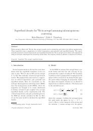
Superfluid 3 He-B Vortex Simulations inside a 

Rotating Cylinder 

R. Hänninen, A. Mitani, and M. Tsubota 

Department of Physics, Osaka City University, 

Sumiyoshi-ku, Osaka 558-8585, Japan 

We study numerically vortex dynamics in superfluid 3 He-B by solving the full 

Biot-Savart equations inside a rotating cylinder. The initial vortex configuration 

seems to have an essential role whether the growth process starts or 

not. The growth process is, at least at the early stages of simulations, mostly 

governed by the reconnections with cylinder boundary. In order to see a 

large increase in vortex density one should go below 0.5Tc in temperature, 

somewhat lower than what is observed in the experiments. 

PACS numbers: 47.32, 67.57. 

1. INTRODUCTION 

The movement of quantized vortices and superfluid turbulence has recently 

been experimentally analyzed in Helsinki by using a rotating 3 He 

cryostat 1 . A small number of vortices are injected into the B phase by using 

a Kelvin-Helmholz instability of the A-B phase boundary and the resulting 

time development of the vortex tangle is analyzed by NMR. 

In a rotating cylinder, counterflow typically forces the vortices to form 

a regular array of rectilinear vortices that finally rotate with the container. 

However, if a vortex line has large enough tangential component along the 

counterflow there may appear Kelvin-waves that eventually can lead to 

instabilities 2–4 . These instabilities together with vortex reconnections favor 

a turbulent state that is seen in experiments at temperatures below 0.6Tc. 

Here we try to explain those experiments by studying numerically the 

vortex dynamics using the full Biot-Savart equations. The problem soon 

encountered was that the results depend essentially on the initial ansatz. 

Therefore we consider here only a few examples and we do not try to give 

any accurate dependences on rotation velocity or temperature.


2. MOTION OF A VORTEX 

An extensive formulation of the vortex dynamics is well described in 

Refs. 5 and 6 by Schwarz and here we only describe the main parts that are 

needed in the formulation of the problem. 

Typically the vortex line is presented in the parametric form by s = 

s(ξ, t) where ξ is the length along the vortex and t is the time. In the 

absence of friction and in an infinite fluid a vortex moves with the local 

superfluid velocity that is given by a well-known Biot-Savart law: 

vs,ω(r, t) = κ 

 

(s1 − r) × ds1 

4π |s1 − r| 3 . (1) 

If one tries to evaluate this expression at point r = s on the vortex one 

notes that the integral diverges. This divergence can be handled and the 

end result is that the velocity of a vortex in the absence of friction is given 

by: 

˙s0 = κ 

4π s′ × s ′′ 

2(l+l−) 

ln 

1/2 

e 1/4 a0 

 

+ κ 

′ 

(s1 − s) × ds1 

4π |s1 − s| 3 + vs,b(s). (2) 

Here the first term on the rhs is the local induction term where l− and l+ 

are the lengths of two adjacent line elements after discretization. Vectors 

s ′ and s ′′ , where the differentiation is with respect to ξ, are tangent and 

principal normal at s. The symbol a0 is the vortex core size that for 3 He-B is 

a0 ≈ 10 −5 mm. The second term is the non-local term where the integration 

is done over the rest of the vortex filament, not connected to the point s. The 

last term on the rhs is included in order to take into account the boundaries. 

It is an additional velocity field that is required to satisfy a zero flow into the 

boundary. Typically the field vs,b can be obtained by using image vortices 

and included in the non-local term. This can be done, for example, in the 

case of plane boundaries. The boundary condition in a cylinder is described 

in more detail below. 

In the presence of mutual-friction the relative velocity between the normal 

fluid and the vortex creates a frictional force, so that the equation of 

motion becomes 

˙s = ˙s0 + αs ′ × (vn − ˙s0) − α ′ s ′ × [s ′ × (vn − ˙s0)]. (3) 

Here the coefficients α and α ′ have been obtained from the experiments 7,8 

and vn is the undisturbed normal fluid velocity far from the vortex core. 

In principle, the motion of the vortex can be followed simply by integrating 

this equation.

Superfluid 3 He-B Vortex Simulations inside a Rotating Cylinder 

2.1. Cylindrical Boundary Condition 

In general the simple method of image vortices cannot be applied in a 

cylinder, but for straight axial vortices this method is applicable. In that 

case each vortex point at (ρ,φ,z) in cylindrical coordinates has an image 

point at (R 2 /ρ,φ,z), where R is the radius of the cylinder. For vortices of 

arbitrary shape one must in general solve the Laplace equation ∇ 2 Φ = 0 

inside the cylinder to find the boundary velocity vb = ∇Φ. 

In our calculations we used image vortices above and below the cylinder 

in order to cancel the flow through the top and bottom faces. The flow 

through the cell (ρ = R) was canceled using both image vortices obtained 

from inversion and using a Fourier series solution for the Laplace equation. 

The method is the same used at least by Zieve and Donev in Ref. 9. The 

reason for using also the image vortex is the following: First the image vortex 

obtained by simply inverting ρ → R 2 /ρ gives in many cases a good 

approximation for the boundary field vb and if one only wants to obtain a 

qualitative picture for the vortex movement it is typically enough. Secondly, 

it reduces the number of terms needed in the Fourier series. However, we 

should note that even if the boundary condition is not always accurately satisfied 

its effect on the vortex movement is typically too small to be observed. 

In the simulations presented here we used a grid of 64×64 points on the cell 

to determine the solution for vb. 

3. NUMERICS AND RESULTS 

In our simulations we used a familiar fourth order Runge-Kutta method 

to follow the time development of our vortex configuration. The time step 

∆t was allowed to vary between 0.1ms and 10ms. It was adjusted to avoid 

difficulties with the reconnections. The maximum ∆t should also be small 

enough since even without dissipation and with ∆t = 5ms a vortex ring of 

radius 0.1mm and described by 30 points travels 1000s without a change in 

vortex length. The spacial resolution was allowed to vary between 0.01mm 

and 0.2mm and was chosen to be more accurate at places where the local radius 

of curvature is small. In order to reduce the cpu-time not all the spacial 

points were used to calculate the Biot-Savart integral. The number of points 

was increased until the required accuracy (typically 98%) was obtained. 

The calculations presented here were done in the laboratory frame where 

the normal fluid velocity is given by vn = Ω×r. Now Ω = Ωˆz and the radius 

of the cell R was chosen to be 3mm. Pressure used was 29bar. In order to 

explain the Helsinki experiments we first considered a quarter loop with 

constant radius that bends from the bottom of the cylinder (z = 0) to the


Fig. 1. Time development (straightening) of a vortex loop with initial radius 

of 1mm in rotating cylinder (R = 3mm and L = 10mm). Time difference 

between two sequential lines is 1s. Figure 1b is a top view of Fig. 1a, where 

T = 0.4Tc and ω = 1.5rad/s. In Fig. 1c we have T = 0.7Tc and ω = 0.2rad/s. 

cylindrical cell wall (ρ = R). However, at all temperatures calculated and 

using the typical rotation velocities of order 1rad/s, the vortex just seems 

to straighten up as seen in Fig.1. So the component along the counterflow 

is never large enough to excite the Kelvin waves that lead to growing of the 

vortex length and together with reconnections to turbulent state. The above 

applies also to several vortices of the same shape. 

If one compares these results with our previous calculations, for example 

in Ref. 4, one might notice that in the previous papers the instabilities occur 

more easily. This is because in those papers the effect of rotation might have 

been taken into account improperly: a more detailed study will be reported 

elsewhere. 

In order to observe the effect of the Kevin waves we did the calculations 

for a vortex ring with radius of 2.5mm at the center of the cylinder (R = 3mm 

and L = 5mm) at z = 2.5mm plane. The rotation velocity was chosen to be 

1.5rad/s. At all temperatures one obtains approximately 20 Kelvin waves 

that can also be seen in Fig. 2. If the ring has fluctuations and is not exactly 

centered around the rotation axis, the creation of Kelvin waves is faster but

Superfluid 3 He-B Vortex Simulations inside a Rotating Cylinder 

Fig. 2. Time development of a vortex ring inside a rotating cylinder (R = 

3mm, L = 5mm, and ω = 1.5rad/s) at T = 0.4Tc. Initially the ring is at z 

= 2.5mm plane and has radius of 2.5mm. The dashed line in the upper left 

figure shows the initial configuration before the Kelvin waves are developed. 

more inhomogeneous. At high temperatures the resulting growing spiral 

reconnects to the cylinder boundary and results in about 20 vortices that 

eventually form a vortex lattice at the center of the cylinder. At T = 0.4Tc 

we observed that appearance of Kelvin like waves continues also after this 

first cycle near the cylinder boundary. Even if most of the vorticity is driven 

to the center of the cylinder the reconnections mostly with the boundary 

create new vortices and in 30 seconds about 300 vortices are created, which 

can be seen in Fig. 2. The characteristic time for the vortex growth is mainly 

determined by mutual friction but also by rotation velocity. The time when 

the vortex number really starts to increase is additionally strongly affected 

by the initial vortex configuration.


We also have simulations running where initially 11 vortex loops bend 

from the bottom of the cylinder to the cell accompanied by 6 small elliptical 

rings above them at ω = 1.0rad/s. Also in that case the results indicate that 

the critical temperature, below which a turbulent state can be observed, lies 

between 0.4Tc and 0.5Tc. 

4. CONCLUSIONS 

In summary, we argue that the initial vortex configuration has a strong 

influence on whether turbulence is created in a rotating cylinder or not. A 

turbulent tangle is observed only at considerably lower temperatures than 

what is observed in experiments. However, we still need more simulations 

in order to see the right dependence on temperature and rotation velocity. 

We also have to consider the boundary condition for the vortices at the 

phase boundary more carefully, since in order not to disturb the vortex 

configuration on the A-phase side a vortex is likely to be pinned at the 

phase boundary. This would imply a larger component along the flow and 

more Kelvin waves. 

ACKNOWLEDGMENTS 

We wish to thank W.F. Vinen, A.P. Finne, M. Krusius and E.V. Thuneberg 

for fruitful discussions. 

REFERENCES 

1. A.P. Finne, T. Araki, R. Blaauwgeers, V.B. Eltsov, N.B. Kopnin, M. Krusius, 

L. Skrbek, M. Tsubota, and G.E. Volovik, Nature 424, 1022 (2003). 

2. R.J. Donnely, Quantized Vortices in Helium II (Cambridge University Press, 

Cambridge, England, 1991). 

3. C.E. Swanson. C.F. Barenghi, and R.J. Donnelly, Phys. Rev. Lett. 50, 190 (1983). 

4. M. Tsubota, T. Araki, and C.F. Barenghi, Phys. Rev. Lett. 90, 205301 (2003). 

5. K.W. Schwarz, Phys. Rev. B 31, 5782 (1985). 

6. K.W. Schwarz, Phys. Rev. B 38, 2398 (1988). 

7. T.D.C. Bevan, A.J. Manninen, J.B. Cook, A.J. Armstrong, J.R. Hook, and H.E. 

Hall Phys. Rev. Lett. 74, 750 (1995). 

8. T.D.C. Bevan, A.J. Manninen, J.B. Cook, H. Alles, J.R. Hook, and H.E. Hall, 

J. Low Temp. Phys. 109, 423 (1997). 

9. R.J. Zieve and L.A.K. Donev, J. Low Temp. Phys. 121, 199 (2000).

Proceedings of QFS2004 - Low Temperature Laboratory

Create successful ePaper yourself

Delete template?

Save as template?