ICON-EDiT ICON-EDiT

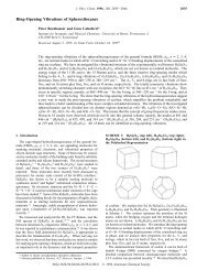
Extended Hückel Molecular Orbitals and Oscillator Strength
Calculations
ICON-EDiT
Manual written by
Gion Calzaferri, Stephan Glaus, Dominik Brühwiler
ICON-EDiT
Program written by
Ruedi Rytz, Stephan Glaus, Martin Brändle,
Dominik Brühwiler and Gion Calzaferri
Department of Chemistry and Biochemistry
University of Berne, Freiestrasse 3, CH-3012 Bern
Berne, Summer 2000

1 Introduction
ICON-EDiT is a FORTRAN program package that performs extended-Hückel molecular orbital and
oscillator strength calculations on molecules.
s,p,d orbitals, a two-body repulsive energy term, options for different Wolfsberg-Helmholz formulas,
charge iteration procedures, population analysis, FMO (fragment molecular orbitals), geometry
variation, energy minimization and oscillator strength calculations are included.
ICON-EDiT consists of four parts, INPUTC, ICONC, EDiT and GOP.
The INPUTC part of the program is a self-explanatory input program. It reads the necessary input
parameters from the ASCII data files ATOMDEF.DAT, VOI.DAT and FOI.DAT that can be extended
and/or adapted to meet the requirements of the user.
ICONC performs extended-Hückel calculations on files created by INPUTC.
EDiT allows to calculate oscillator strengths of electronic dipole-induced transitions (EDiTs) based
on Slater-type extended-Hückel wave functions.
GOP searches for a minimum in an energy hyper surface using INPUTC and ICONC with files created
by INPUTC for input.
ICON-EDiT runs under Windows NT, however, no machine specific specialties have been included.
2
ICON-EDiT, Summer 2000 Gion Calzaferri

2 Package
The extended-Hückel part of ICON-EDiT is an updated version of ICONC&INPUTC. [1] ICON8, [2]
FMO, [3] GENINS and CONVERT provided by the ROALD HOFFMANN group have been used as bases for
ICON-EDiT which includes among other new features an ASED procedure. [4] EDiT is a program to
calculate oscillator strengths of electronic dipole-induced transitions (EDiTs) based on the EHMO
Slater-type wave functions generated by ICONC&INPUTC. [5]
2.1 Contents
The package consists of the FORTRAN sources FILENAME.F, the corresponding FILENAME.EXE
files, the data files FILENAME.DAT and some examples FILENAME.GEN, FILENAME.MO and
FILENAME.KAR. The 32-bit extender programs DOSXMSF.EXE and DOSXNT386.EXE are
included for those wishing to run the binaries under DOS and/or Windows 3.x.
2.1.1 Source files
3
The source codes of INPUTC, ICONC and EDiT are split into their subroutines, the source code of
GOP is distributed in modules. All sources are located in the respective subdirectories of the directory
SOURCES.
With the exception of GOP, the programs have already been compiled on different platforms such as
VAX/VMS, IBM RS/6000, DEC/ALPHA, LINUX, DOS/WINDOWS and many more. No problems
have been reported so far. However, a few points should be noted:
If you wish to compile the programs with the VAX FORTRAN make sure to change the carriage
control character „\” to „$” in the FORMAT statements.
The Machine constants used in the Eigenvalue solve engine GIVENS.FOR should be adapted to the
requirement of your computer. The correct machine constants for MSDOS, VAX and IBM RS/6000
are included in the respective file. The user only has to unmark the corresponding lines in this
subroutine.
All three programs have been designed to contain the user changeable parameters in their proper
parameter files which are ICONPARA.FOR, INPUPARA.FOR and EDPARA.FOR. The parameters
listed therein should be adaptable to the requirements of the user and/or the available resources,
such as computer memory. The maximum number of atoms (variable MXATOM) has been tested for
up to 999. We do not guarantee correct results, if you push this limit beyond.
GOP uses a compiler-specific routine to access the operating system. You will have to change the
file ‘INPUTC_ICONC.f90’ to compile the program with your own compiler.
The program-package is available at no charge. As a consequence no responsibility and no
support can be provided by the authors..
ICON-EDiT, Summer 2000 Gion Calzaferri

2.1.2 Executables
INPUTC.EXE reads the data files ATOMDEF.DAT, VOI.DAT and FOI.DAT which must be located
in the same directory as the binary itself. Its purpose is to output either a cartesian coordinate file
(FILENAME.KAR) or an internal coordinate file (FILENAME.GEN) depending on the choice you
have made (cf. Chapter 2.2). As ICONC is designed to work with cartesian coordinates only, the .gen
files can be converted to the temporary files TEMP.VAR and TEMP.KAR. The memory requirement is
rather small ( » 180 kBytes).
The FILENAME.GEN and the TEMP.KAR files are the input files for ICONC.
ICONC.EXE is the actual extended-Hückel molecular orbital (EHMO) program. The memory
requirement is » 6.5 MBytes for a DOS/Windows 3.x binary compiled for 100 atoms (cf. variable
MXATOM in ICONPARA.FOR).
EDiT.EXE calculates electronic dipole-induced transitions between an initial molecular orbital Ψi and
a final MO Ψf. Besides the files FILENAME.MO and FILENAME.GEN that are related to the ICONC
program, EDiT needs an input file FILENAME.EDI that has to be created seperately in an ASCII editor
of your choice. A binary dimensioned for 100 atoms (and up to 400 AOs) uses about 4.5 MBytes of
RAM.
GOP.EXE searches for a minimum on an energy hyper surface of a molecule specified in a .gen file.
The user may choose which properties of the molecule to include in a calculation and which not. GOP
itself uses practically no resources, but it makes calls on INPUTC and ICONC, so the memory
requirement is the same as for them.
DOS/Windows 3.x specialties:
The DOS/Windows 3.x binaries have been created using the Microsoft FORTRAN PowerStation compiler. In order
for the 32-bit binaries to run on a 16-bit operating system the respective 32-bit extender programs are included in
this distribution. These are DOSXMSF.EXE and DOSXNT.386, respectively (DOSXMSF.EXE being the proper
extender program). If you intend to use these programs under DOS only, you can forget about DOSXNT.386.
DOSXMSF.EXE should be copied to a location stated in your PATH environment (i.e. to the current working
directory). If you plan to run the programs under Windows 3.x in a DOS shell you should add the line
DEVICE=X:\SOMEPATH\DOSXNT.386
to the [Enh386] section of your SYSTEM.INI file.
The program consuming the most memory is ICONC. Depending on the configuration of your PC (different drivers,
SMARTDRIVE, RAMDISK, etc.) 8 or 16 MBytes of RAM should allow to run ICONC without needing to access
virtual memory. If you have less built-in physical memory you can still run the programs by allowing the programs
to page out parts of its image to the hard disk. Virtual memory will be accessed on the drive where
DOSXMSF.EXE is located. This will NOT work on a compressed drive. Therefore, if you have DriveSpace installed
you may want to relocate the swap space by adding something like
SET DOSX = SWAPDIR X:\MYSWAP
4
to your AUTOEXEC.BAT file. However, if you run the programs under Windows 3.x in a DOS shell, Windows will
take care of your virtual memory. Size and properties can then be adjusted by starting the control panel application
and selecting the 386 Enhanced icon. Do NOT run ICON-EDiT under Windows 3.x unless you are sure to have
enough free RAM.
ICON-EDiT, Summer 2000 Gion Calzaferri

2.1.3 Data Files
ATOMDEF.DAT is needed by INPUTC. It contains the atomic symbols, the number of valence
electrons, the quantum numbers of the orbitals, the corresponding Slater exponents and the Coulomb
integrals. For most of the main group elements the quantum number ND has been chosen equal to 0. A
quantum number of 0 means that the corresponding atomic orbital is skipped. To include d orbitals ND
= 0 has to be substituted with ND = 3, 4 or 5 depending on the period to which the atom belongs.
Special notation: atomic symbols followed by M, -, 1, 2 or 3 have the meanings: metal, anion, cation, higher oxidation
states.
Be careful! It is wise to check whether the parameters are well suited to your problem.
ATOMDEF.DAT can easily be changed or extended according to the special needs of the user. Be
careful not to change the format. The number of atoms that can be defined is limited to 150.
FOI.DAT is needed by INPUTC. It contains the charge iteration parameters of the transition elements.
VOI.DAT is needed by INPUTC. It contains the charge iteration parameters of the main group
elements.
2.1.4 Contents of the distribution
The .zip files (also available as .tar.gz files) can be downloaded from the following website:
http://iacrs1.unibe.ch/members/iconedit.html
NT-bin.zip sources.zip
examples.zip
q-tools.zip
INPUTC.EXE
ICONC.EXE
EDiT.EXE
GOP.EXE
ATOMDEF.DAT
FOI.DAT
VOI.DAT
INPUTC (DIR)
ICONC (DIR)
EDiT (DIR)
GOP (DIR)
containing the sources
5
2-H2O_GOP.GEN
2H2OAG_ANGLE.GEN
2H2OAG_DISTANCE.GEN
BENZENE.GEN
BENZENE.OUT
BENZENE1.PGR.GOP
BENZENE1.E_MIN.OUT
BIPY.KAR
BIPY.OUT
C2H2.GEN
C2H4.GEN
C60.GEN
CH4.GEN
CH4.MO
CH4.OUT
GLYCIN.KAR
GLYCIN.OUT
H2.GEN
H2.OUT
H2O.KAR
H2O.OUT
H2O_GOP.GEN
MNO4-.EDI
MNO4-.EDO
MNO4-.EDS
MNO4-.GEN
MNO4-.MO
MNO4-.OUT
NICO4IT.KAR
NICO4IT.OUT
PROPEN_F.GEN
PROPEN_F.OUT
Q-TOOLS.EXE
SAMPLES(DIR)
Containing some examples.
Refer to the description of
Q-TOOLS
ICON-EDiT, Summer 2000 Gion Calzaferri

2.2 INPUTC
INPUTC is a self-explanatory FORTRAN program which produces files used as input for the EHMO
program ICONC.EXE. You may select between different coordinate types for the input of molecules as
well as between different options for the EHMO calculation.
ICONC accepts only input files with atom positions in cartesian coordinates. INPUTC converts
internal coordinates to cartesian coordinates.
INPUTC needs the parameter files ATOMDEF.DAT, VOI.DAT and FOI.DAT. These files must be in
the current working directory.
To start the program type INPUTC at the command line prompt.
The program will then ask for the type of input you want to make. The questions are:
1 Cartesian coordinates
2 Internal coordinates (with variations)
3 Conversion of a file from #2 (.GEN file)
0 End
6
Option 1 asks for input of the atomic positions in Cartesian coordinates. A file with the extension
.KAR is then written to the hard disk. Input files in Cartesian coordinates (e.g. name.KAR files) can be
used for ICONC calculations without conversion.
Option 2 asks for the atomic positions in internal coordinates. Besides the fact that internal coordinates
are often useful and allow a much easier setup of molecular geometries from known data such as bond
angles and bond lengths, INPUTC supports automatic geometry variation for this type of coordinates. In
a first step INPUTC dumps an internal coordinate file with the extension .GEN to the hard disk. It then
varies the geometries and writes its output to the temporary files TEMP.VAR and TEMP.KAR. These
files are temporary in the sense that they will be overwritten the next time you choose either option 2
or 3. As the .GEN files contain variation information in a condensed form you may wish to keep these
files only. The TEMP.KAR files needed as input for ICONC can be generated from the respective
.GEN file at any time by choosing option 3. The TEMP.VAR files contain the varied internal
coordinates what is handy to check the success of geometry variation. We now briefly discuss the
setup of internal coordinate geometries.
The first atom 1 in Figure 1 defines the origin. If you choose an angle α of ±180 o the second atom 2
lies on the Z-axis in positive direction. For a dihedral angle of 0 o or 180 o the third atom is in the
XZ-plane. To set up the coordinate system and/or any reference point the user can create dummy
atoms. Dummy atoms are automatically removed from calculation; they have to be given the highest
numbers. Hence, if you consider a molecule consisting of N atoms the first dummy atom has to be
labeled with N+1. Sequencing of atoms for counting is determined by only the real (excluding dummy)
atoms. You can only point once to the same atom but you can point from a selected atom to other
atoms as often as you like. The bond angle is the angle between the vector b and the connection
between the two atoms 1 and 2. The dihedral angle ξ is the angle between the last defined plane and
ICON-EDiT, Summer 2000 Gion Calzaferri

the new vector to be defined. At the beginning the XZ-plane is defined by the vectors a and b. Please
note that the dihedral angle is associated with the vector K - L.
We further explain the use of the above definitions by adding a few examples.
If atom 1 is located at position (x=0, y=0, z=0) the input in internal coordinates (r,α,ξ) must be (0,0,0).
If then atom 2 is located at (x=0, y=1, z=0) the input must be (1,180,0) and so on.
L
K
J
I
Z
23
2
1
Y
b
3
a
12
= 180
L I
= Bond angle = Dihedral angle
7
Figure 1: Definition of the bond angle α and the dihedral angle ξ. In case of atoms 1 and 2 in the upper
scheme K corresponds to atom 1.
ICON-EDiT, Summer 2000 Gion Calzaferri
K
J
X

Figure 2: EXAMPLE 1, D2h H4
number of atoms
number of dummy atoms
number of vectors
b
r
14
D2h point group; e.g. D2h H4
4 atoms and three connections
4
r 14
=
r 23
1 r
2
12
4
0
3
3
r
23
8
vector
If we want to place the four atoms in the x,y plane, so that the z axis coincides with the C4 axis, the
following input will do it:
ICON-EDiT, Summer 2000 Gion Calzaferri
1 2
2 3
1 4
vector
5 1
1 2
2 3
3 4
atom
1
2
3
4
5=dummy
distance
2
2
2
distance
0,707107
1
1
1
x
0,7071
0
-0,7071
0
0
α
180
90
90
α
90
45
90
90
y
0
0,7071
0
-0,7071
0
ξ
0
0
0
ξ
0
90
0
0
z
0
0
0
0
0

The following input places the four atoms into the y,z plane, so that the x axis coincides with the C4
axis:
Figure 3: EXAMPLE 2, Td CH4
5
vector
5 1
1 2
2 3
3 4
atom
1
2
3
4
5=dummy
number of atoms
distance
0,707107
1
1
1
x
0
0,7071
0
-0,7071
0
number of dummy atoms
number of vectors
X
4
Y
1
2
3
α
180
45
90
90
y
0
0
0
0
0
5
0
4
Z
ξ
0
0
0
0
z
0,7071
0
-0,7071
0
0
9
vector
0
a
-a
a
-a
a=0.6293
ICON-EDiT, Summer 2000 Gion Calzaferri
1 2
1 3
1 4
1 5
Atom
1
2
3
4
5
distance
1.090
1.090
1.090
1.090
x
0
a
-a
-a
a
α
125.2644
125.2644
54.7356
54.7356
y
ξ
45.0
225.0
135.0
315.0
z
0
a
a
-a
-a

Figure 4: EXAMPLE 3, D6h-benzene
This example illustrates how to place the z-axis perpendicular to the plane of a molecule with Dnh
symmetry, so that the Cn axis coincides with the z-axis. If you choose the coordinate system in this way,
ICONC will deliver symmetry adapted wave functions.
number of atoms
number of dummy atoms
number of vectors
12
1
12
Internal coordinates, number 13 is the dummy atom:
13 1 1.40 90.0 .0 places atom 1 on the x axis at position 1.4
1 2 1.40 60.0 90.0 rotation from the (x,z) plane to to(x,y) plane
2 3 1.40 120.0 .0
3 4 1.40 120.0 .0
4 5 1.40 120.0 .0
5 6 1.40 120.0 .0
1 7 1.06 180.0 .0
2 8 1.06 240.0 .0
3 9 1.06 240.0 .0
4 10 1.06 240.0 .0
5 11 1.06 240.0 .0
6 12 1.06 240.0 .0
* C C C C C * H H H H H
Resulting cartesian coordinates:
1 1.400000 .000000 .000000
2 .700000 1.212436 .000000
3 -.700000 1.212436 .000000
4 -1.400000 .000000 .000000
5 -.700000 -1.212436 .000000
6 .700000 -1.212436 .000000
7 2.460000 .000000 .000000
8 1.230000 2.130422 .000000
9 -1.230000 2.130423 .000000
10 -2.460000 .000000 .000000
11 -1.230000 -2.130422 .000000
12 1.230000 -2.130423 .000000
* C C C C C * H H H H H
10
ICON-EDiT, Summer 2000 Gion Calzaferri

Figure 5: EXAMPLE 4, Zeise-Salt ((H2C = CH2 ) PtCl3 ), try ZEISE.GEN.
C
H
number of atoms 10
number of dummy atoms D 1
number of vssectors 10
1
2
3
4
5
6
7
8
9
10
H
C
H
vector
number
H
Pt Cl
Cl
Cl
vector
11 1
1 2
1 3
1 4
11 5
11 6
5 7
5 8
6 9
6 10
11
distance
2.090
2.300
2.300
2.300
0.735
0.735
1.080
1.080
1.080
1.080
α
180.0
180.0
90.5
90.5
90.0
270.0
109.5
109.5
109.5
109.5
ξ
0.0
0.0
270.0
90.0
0.0
0.0
90.0
270.0
90.0
270.0
ICON-EDiT, Summer 2000 Gion Calzaferri
9
6
10
D
5
7
8
Y
4
3
1 2
X
Z

Figure 6: EXAMPLE 5, (H2C = CH2) PtCl2N(CH3)2, try CHNCLPT.GEN.
number of atoms
number of dummy atoms D
number of vectors
vector
number
1
2
3
4
5
6
7
8
9
10
11
12
13
14
15
16
17
18
vector
19 1
1 2
2 3
2 4
19 5
19 6
1 7
1 8
5 9
5 10
6 11
6 12
3 13
4 14
3 15
4 16
3 17
4 18
18
1
18
12
distance
2.090
2.020
1.580
1.580
0.735
0.735
2.300
2.300
1.080
1.080
1.080
1.080
1.080
1.080
1.080
1.080
1.080
1.080
α
180.0
180.0
114.0
114.0
90.0
270.0
90.5
90.5
109.5
109.5
109.5
109.5
109.5
109.5
109.5
109.5
109.5
109.5
ξ
0.0
0.0
90.0
270.0
0.0
0.0
270.0
90.0
90.0
270.0
90.0
270.0
270.0
90.0
150.0
330.0
30.0
210.0
ICON-EDiT, Summer 2000 Gion Calzaferri

Figure 7: EXAMPLE 6, 4’ -Phenylterpyridine, try PTPY.GEN.
vector numb er
1
2
3
4
5
6
7
8
9
10
11
12
13
14
15
16
17
18
19
20
21
22
23
24
25
26
27
28
29
30
31
32
33
34
35
36
37
38
39
40
vector
40 1
1 2
2 3
3 4
4 5
5 6
6 7
7 8
8 9
9 10
10 11
11 12
2 13
13 14
14 15
15 16
16 17
17 18
4 19
19 20
20 21
21 22
22 23
23 24
22 25
20 27
21 26
3 28
5 35
8 36
9 37
10 38
11 39
14 29
15 30
16 31
17 32
23 33
24 34
24 24
13
distance
2.000
1.352
1.395
1.395
1.395
1.395
1.489
1.395
1.395
1.395
1.395
1.352
1.489
1.395
1.395
1.395
1.395
1.352
1.489
1.395
1.395
1.395
1.395
1.395
1.084
1.084
1.084
1.084
1.084
1.084
1.084
1.084
1.084
1.084
1.084
1.084
1.084
1.084
1.084
1.084
number of atoms = 39
number of vectors = 39
number of dummy atoms = 1
D = dummy atom. The dummy atom(s) must have
the last number(s).
α
180.000
243.325
116.675
120.000
120.000
120.000
240.000
240.000
120.000
120.000
120.000
116.675
236.675
120.000
240.000
240.000
240.000
243.325
240.000
240.000
120.000
120.000
120.000
120.000
240.000
240.000
240.000
240.000
240.000
240.000
240.000
240.000
240.000
120.000
120.000
120.000
120.000
240.000
240.000
240.000
ICON-EDiT, Summer 2000 Gion Calzaferri
ξ
0.0
0.0
0.0
0.0
0.0
0.0
0.0
0.0
0.0
0.0
0.0
0.0
0.0
0.0
0.0
0.0
0.0
0.0
0.0
0.0
0.0
0.0
0.0
0.0
0.0
0.0
0.0
0.0
0.0
0.0
0.0
0.0
0.0
0.0
0.0
0.0
0.0
0.0
0.0
0.0

Figure 8: EXAMPLE 7, H8 Si8 O12, try H8SI8O12.GEN.
8
4
number of atoms
number of dummy atoms D
1
5
3
number of vectors
28
D is number 29 in the centre of the cage.
vector
number
1
2
3
4
5
6
7
8
9
10
11
12
13
14
15
16
17
18
19
20
21
22
23
24
25
26
27
28
7
2
vector
6
29 9
29 10
29 11
29 12
29 13
29 14
29 15
29 16
29 17
29 18
29 19
29 20
29 1
29 2
29 3
29 4
29 5
29 6
29 7
29 8
1 21
2 22
3 23
4 24
5 25
6 26
7 27
8 28
28
1
28
24
2.64428
2.64428
2.64428
2.64428
2.64428
2.64428
2.64428
2.64428
2.64428
2.64428
2.64428
2.64428
2.69795
2.69795
2.69795
2.69795
2.69795
2.69795
2.69795
2.69795
1.45
1.45
1.45
1.45
1.45
1.45
1.45
1.45
20
14
distance
9
16
13
12
17
25
21
α
23
27
10
19
14
15
11
135.0
135.0
135.0
135.0
45.0
45.0
45.0
45.0
90.0
90.0
90.0
90.0
125.2644
125.2644
125.2644
125.2644
54.73561
54.73561
54.73561
54.73561
180.0
180.0
180.0
180.0
180.0
180.0
180.0
180.0
18
22
26
ξ
0.0
90.0
180.0
270.0
0.0
90.0
180.0
270.0
45.0
135.0
225.0
315.0
45.0
135.0
225.0
315.0
45.0
135.0
225.0
315.0
0.0
0.0
0.0
0.0
0.0
0.0
0.0
0.0
ICON-EDiT, Summer 2000 Gion Calzaferri

After this you will be asked: „Do you want to define additional parameters?” Answering Y will show
you the next menu:
1 Charge iteration
2 Controlling output options
3 Orbital occupation
4 Individual 1+k, d parameters
5 Weighted Wolfsberg-Helmholz formula
6 Simple Wolfsberg-Helmholz formula
7 FMO (Fragment Molecular Orbital) Calculation
8 Omit atoms from repulsion energy calculation
9 Exit
REMARK 1
REMARK 2
K = 1 + ✗ $
15
The default option for calculating the off-diagonal elements is the distance dependent
formula:
exp(−✑(R − d0))
q
q = 1 + ([(R − d0) − R − d0 ] $ ✑) 2
with ✗ = 1 and ✑ = 0.35
Option 4 allows to define other κ, δ parameters.
It also allows to define individual κ, δ values for specified atom pairs.
Charge iteration can be carried out at a single atom, at a few atoms or at all
atoms.
The experience shows that it is in general not necessary to carry out charge
iteration for organic molecules, but in some cases it is important.
As a rule charge iteration should be applied at approximately the equilibrium
geometry only. The thus obtained parameters can then be used for all the other
calculations, see e.g. refs [6-7] and [9].
In general it is not necessary to carry out charge iteration at different
geometries, a procedure which is usually time consuming.
In some cases it is, however, important to carry out charge iteration at each
geometry investigated; see e.g. ref. [6-7].
ICON-EDiT, Summer 2000 Gion Calzaferri

REMARK 3
REMARK 4
REMARK 5
REMARK 6
If calculations are performed for varying geometries, MOBY output is only
generated for the last geometry. MOBY output generates connectivity
information that has to be regarded as a proposal only and may have to be
changed by the user. MOBY output files have the extension .mo. They serve as
input files for the programs MOBY and EDiT.
To calculate the sum
✟ b0 s s Es
0 and ERep
16
Option 2 includes the following possibilities for controlling the output of
ICONC:
1 Coordinates and parameters
3 Distance matrix
4 Overlap matrix
5 Madelung parameters
6 Hückel matrix
8 Energy levels
9 Total energy
10 Wave functions
11 Density matrix
12 Overlap population matrix
13 Reduced overlap population matrix
14 Complete charge matrix
15 Reduced charge matrix
16 Net charges and populations
17 Energy matrix
18 Reduced energy matrix
19 Energy partitioning
20 Reduced energy partitioning
21 Core-core repulsion energy matrix
22 Moby output
25 Exit
by means of eqs. (3) and (51) respectively, the valence electrons of the atoms
are filled into the energetically lowest levels according to the Aufbau
principle. The thus resulting electron configuration does in general not
correspond to the electron configuration of the free atoms in case of transition
elements. You can change this by choosing the corresponding switch in Option
2. If charge iteration is used, we recommend to apply the default option.
The easiest way to get familiarized with the program is to try the different
options and to study the results. Perhaps you may also want to try some of the
examples included.
ICON-EDiT, Summer 2000 Gion Calzaferri

REMARK 7
17
The charge iteration parameters are split up in two files; VOI.DAT containing
the parameters for main group elements and FOI.DAT comprising the respective
parameters for transition metals. If you intend to perform charge iteration
on both types of elements you have to choose method B „VSIE-parameters (for
d-elements)” .You will then be asked whether you want to do charge iteration
on all atoms or on selected atoms only. The latter option allows you to specify
the elements you want to charge iterate. In order to have charge iteration on selected
atoms you may want to give the atoms occupying different symmetry positions
different names. You do this by copying the respective rows in
ATOMDEF.DAT, VOI.DAT and/or FOI.DAT and giving the elements different
names (eg. O1 and O2, for two symmetrically distinguishable types of oxygen
atoms, the name must not contain more than 2 letters). Consider for example
CO2. As the needed parameters are already included in VOI.DAT you will
choose method A. If you then choose charge iteration on selected atoms you
will be asked on how many atoms you want to charge iterate. The program proposes
3. As you only have two types of (symmetrically) distinguishable atoms,
select 2! The program then lists the atoms. The oxygen is listed twice as the
program does not know about symmetry. The proposed succession of the atoms
has to be obeyed. Hence, if the program prints the list „O C O", you will have
to select O and then C. Otherwise the oxygen atoms will be charge iteratated
with the carbon parameters, which is of course wrong!
Option 3 converts a previously generated internal coordinate file with the extension .GEN (cf. Option
2) into a Cartesian file named TEMP.KAR.
ICON-EDiT, Summer 2000 Gion Calzaferri

2.3 ICONC
ICONC is a FORTRAN program. It performs extended-Hückel calculations on molecules.
s, p, d orbitals are accepted.
A two-body repulsive energy term is included.
A distance-dependent Wolfsberg-Helmholz constant is used by default. Other options can be chosen.
ICONC can perform FMO calculations.
ICONC accepts input files with atom positions in Cartesian coordinates only. The easiest way to use
the programs is to first apply INPUTC which creates the *.KAR files that ICONC accepts as its input.
To start the program type ICONC < filename.KAR > filename.OUT
18
The „” signs are essential. They redirect standart input and standard output of ICONC. The
standard input will be read from filename.KAR while the standard output will be written to
filename.OUT.
REMARK: The calculated wave functions are usually not symmetry adapted. For the degenerate
orbitals of highly symmetric molecules this may cause the wave functions difficult to interpret. To get
symmetry adapted wave functions, appropriate rotation has to be carried out. It is always possible,
however, to solve the problem by inducing a small appropriate antisymmetric distortion. Appropriate
distortions are distortions which remove specific or all C3 axis of rotation.
In addition to the filename.OUT ICONC creates the two temporary files ENERNI.DAT and
ENERTOT.DAT. ENERNI.DAT contains the number of orbitals and the orbital energies.
ENERTOT.DAT contains the VARIED BOND LENGTHS OR BOND ANGLES, the SUM OF
ONE-ELECTRON ENERGIES, the ORBITAL STABILIZATION ENERGY, the TWO-BODY
REPULSION ENERGY and the STABILIZATION + REPULSION ENERGY. These files are often
very useful. If for example you want to draw an energy hypersurface, all the needed information is
contained in ENERTOT.DAT.
The output option MOBY creates in addition a file filename.MO. The *.MO files were originally
introduced to meet the requirements of the molecular modeling package MOBY by Udo Höweler,
Springer Verlag Berlin, 1993. We then found these files convenient for the EDiT program as well.
ICON-EDiT, Summer 2000 Gion Calzaferri

2.4 EDiT
EDiT is a FORTRAN program that performs oscillator strength calculations of electronic
dipole-induced transitions (EDiTs) based on EHMO wave functions generated by ICONC.
To start the program type
19
EDiT.bat filename
The filename(.EDI) is the EDiT input file, that will be created by the ICONC program (Output control
parameter #23 → False) and has to be modified with an ASCII text editor of your choice. The different
options that determine the run-time behaviour of EDiT can be chosen by stating the respective
KEYWORDs in filename.EDI. The text below written in Courier is a sample input file set up to
calculate the first electronic transition in permanganate. Please refer to this file which is also included
in the distribution to get a brief overview of the possible keywords.
!%%%%%%%%%%%%%%%%%%%%%%%%%%%%%%%%%%%%%%%%%%%%%%%%%%%%%%%%%%%%%%%%%%%%%%%%
!
! mno4-.edi - Input file for oscillator strength calculations with EDiT
!
! %%Creator: ICONC
!
! %%Usage: EDiT < mno4-.edi > mno4-.log
!
! %%Keywords:
! OUTFILE=??? - Output file is mno4-.eds.
! SPECFILE=??? - Corrected line spectrum file for smoothing is mno4-.eds.
! OSCILLOUT - Print the oscillator strengths.
! DIPLENOUT - Print the transition dipole lengths.
! MATOUT - Print the transition dipole matrices.
! FITONLY - Do Gaussian smoothing only.
! MATRICE=ALL - ALL transition matrix elements are taken into account.
! CUTOFF=xx.x - Cutoff length for off block diagonal elements is 10.0 A.
! POL = XYZ - X, Y, and Z transitions considered.
! CORRECT - Correction for degeneracies is done with TOL = 0.0001 eV.
! VERBOSE - Print verbose output to log file.
!
!%%%%%%%%%%%%%%%%%%%%%%%%%%%%%%%%%%%%%%%%%%%%%%%%%%%%%%%%%%%%%%%%%%%%%%%%
!
TITLE Electronic Transitions in Mno4-
!
! The files
KEYWRD OUTFILE=mno4-.edo
KEYWRD SPECFILE=mno4-.eds
!
! Output
KEYWRD OSCILLOUT
KEYWRD DIPLENOUT
!KEYWRD MATOUT
!
!KEYWRD FITONLY
!
! Method
KEYWRD MATRICE=ALL
!KEYWRD CUTOFF=10.0
!
! Polarization
KEYWRD POL = XYZ
KEYWRD CORRECT, TOLERANCE=0.0001
!
! Verbose output to log file
KEYWRD VERBOSE
!
[WAVERANGE]
! Change these numbers to something more reasonable :-)
ICON-EDiT, Summer 2000 Gion Calzaferri

START 4711, 4711
END 4711, 4711
!
[FIT_SPEC]
E_RANGE 20000.0, 40000.0
H_WIDTH 750.0
POINTS 20000
SPECS X, Y, Z, XYZ*
!
![DOT]
!E_RANGE 20000.0, 40000.0
!DELTA_E 10.0
!
!
! No changes should be necessary below here.
!------------------------------------------------------------------------------
[ATOMS]
MN .0000 .0000 .0000
O 9180 .9180 .9180
O -.9180 -.9180 .9180
O -.9180 .9180 -.9180
O .9180 -.9180 -.9180
[ATOMS_END]
[STO]
MN 4s. 4p. 3d.
1.6500 1.0000 .0000 .0000
1.1500 1.0000 .0000 .0000
5.1500 .5470 2.1000 .6050
O 2s. 2p.
2.5750 1.0000 .0000 .0000
2.2750 1.0000 .0000 .0000
O 2s. 2p.
2.5750 1.0000 .0000 .0000
2.2750 1.0000 .0000 .0000
O 2s. 2p.
2.5750 1.0000 .0000 .0000
2.2750 1.0000 .0000 .0000
O 2s. 2p.
2.5750 1.0000 .0000 .0000
2.2750 1.0000 .0000 .0000
[STO_END]
[WAVE_FUNCTIONS]
21.994005 1
1.277633 .000000 .000000 .000000 .000000 .000000 .000000 .000000
.000000 -.458772 .141484 .141484 .141484 -.458772 -.141484 -.141484
.141484 -.458772 -.141484 .141484 -.141484 -.458772 .141484 -.141484
-.141484
.
.
.
.
.
.
20
To calculate the electronic dipole-induced transitions the program needs the Slater exponents, the
geometry information and the final and initial wave functions. All these data is stored in the *.EDI file
and is written on request by ICONC (Output control parameter #23 → False). After running the ICONC
calculation you should make sure that the filename.EDI was written. Then you can modify the
parameters and options directly in the file. Especially you have to define the waverange in which the
electronic dipole-induced transitions should be calculated.
REMARK: As MS-DOS does not distinguish between capital and lower case letters the EDiT
program may conflict with the proper MS-DOS editor EDIT.COM in the sense that EDiT will be
called first. EDiT will then show its heading information and wait for input which it probably won’t
get as one usually does not start a full screen editor by redirecting a file to it. If this should happen just
press CTRL-C to abort EDiT. If this should be a stumbling-block you have the choice of either
renaming EDiT.EXE to EDiTOr.EXE (Electronic Dipole-induced Transitions by the use of Slater-type
Orbitals) or starting the DOS editor by typing EDIT.COM somefile.*.
ICON-EDiT, Summer 2000 Gion Calzaferri

2.5 G O P
The Graphic Optimization Program (GOP) is a FORTRAN 90 program which searches for a minimum
in an energy hyper surface using INPUTC and ICONC. In the current version, a simplex algorithm is being
used (see ‘Algorithm used’ for detail).
In contrast to the other programs in this package, GOP is NOT portable, because it needs to make calls to INPUTC and
ICONC using the operating system. If you want to compile the program yourself, you may have to change the source file
INPUTC_ICONC.f90 (all other source files conform to the FORTRAN 90 ANSI standard).
Input for GOP is provided through a .gen file which must be created using INPUTC before running
GOP. It lets you specify which angles and distances of the molecule specified in the .gen file you want
to include in the optimization process.
GOP needs ICONC and INPUTC with all their needed parameter files. These files must be in the current
working directory.
To start the program type GOP at the command line prompt.
The program will ask for the name of the .gen file you want to use for calculation. You can enter an entire
path, up to 45 characters, including the filename, but leave away the extension .gen. If GOP can’t
locate or access the specified file, it will exit with an error message.
Note that GOP won’t make any changes to your .gen file, but uses a temporary .gen file, named
‘temp$1.gen’ or similar.
After you have specified the .gen file, the main menu will appear:
******************************************
* simplex search for energy minimum *
* *
* 1 use variations in .gen file to *
* choose the parameters *
* 2 choose parameters individually *
* 0 exit *
******************************************
Option 1:
GOP will take the parameter for the energy hyper surface from the variations in the specified .gen file.
Take the following .gen file as example:
2 3 2 2
2 0 2 0
water-corrected values
0 3 0 0 0 1FFFFFFTFF 1.95 .000 .000FFFFFFFFFFFFFFFFFFFFFF
.400000
1 2 .95700 .00000 .00000
1 3 .95700 104.60000 .00000
* * H
O 6 22.5750-28.87 22.2750-13.00
H 1 11.3000-15.79
1
2 3 1.10000 .40000
111 2 2 1.000000
111 2 1 1.000000
111 1 1 1.000000
21
ICON-EDiT, Summer 2000 Gion Calzaferri

It contains three variations, the first changing the bonding angle (H-O-H), the second and third
changing the two distances between O and H. Therefore GOP will optimize a three-dimensional
energy hyper surface, E(α(H-O-H), d(OH1), d(OH2)).
Please note that GOP will uncouple all coupled variations! If the variations in the above .gen file
should look like
111 2 2 1.000000
111 2 1 1.000000
111 * 1 1 1.000000
meaning that the two distances are varied together, the hyper surface optimized by GOP will still be
three-dimensional.
The number of variations and the increment are ignored by GOP.
If you choose this option, you will get to the menu ‘settings for simplex algorithm’ (described below).
Option 2:
With this option, GOP lets you specify which properties of which vectors in your .gen file to use as
parameters for the energy hyper surface.
First you will be asked to enter the number of parameters you want to optimize. If you type in a number
< 1, no calculation will be performed.
Then GOP will ask you to specify the vector and the type of change for each parameter (distance, bond
angle, dihedral angle).
Note that GOP will accept impossible inputs (like -1 for a vector), but this may lead to exceptional
program termination, endless calculation or strange results.
Then you will get to the menu ‘settings for simplex algorithm’:
******************************************
* settings for simplex algorithm *
* *
* 1 use default settings *
* 2 choose individual settings *
******************************************
Option 1 will leave the following default settings:
starting values for parameters: taken from the specified .gen file
initial step sizes: 0.05 for distances, 1.0 for angles
stopping criterion: 1.e-4
maximum number of function evaluations: 500
name of output file: E_MIN.OUT
progress report is disabled
Option 2 will let you change all of these settings.
Note that all inputs you make must conform to FORTRAN:
decimal numbers must be written with a point (not comma)
if you want to type a decimal with an exponent, you must write a decimal point:
1.e-4 means 0.0001; 2.3e3 means 2300 etc., but 1e2 is illegal.
Explanation of the settings:
22
ICON-EDiT, Summer 2000 Gion Calzaferri

starting value for parameters: These determine where the optimization routine starts the search for the
minimum. If you have a more or less vague idea where the minimum could be, set the starting values
accordingly. The number of calculations GOP has to make to find a minimum depends strongly on them.
Different starting values can lead to different minimums or to no minimum at all.
initial step sizes: These determine how far off the starting point the first few calculations will be
made. The default values should be quite reasonable in most cases. But if you start close to a minimum
you may want to choose smaller step sizes to ensure you don’t go away from it with the first few steps.
Also, if you are close to the minimum with just one parameter, you may make its step size small.
Example: You may know that in a water molecule the distances (O-H) are about .958 Å, but have no
idea about the bonding angle. So you will set the initial value for the distances to .958 and choose a
step size of .0005, and for the angle start at 90° with a step size of 2 or even 5.
stopping criterion: This determines to what precision the minimum is searched. It should not be
smaller than about 1.e-10 to make sure no rounding errors are made. Note that the maximum precision
for distances and angles provided by INPUTC is five decimals. A too high precision of the energy
value may not be sensible.
maximum number of function evaluations: The program stops after it has calculated more points than
specified by this number, even if no minimum is found.
name of output file: specifies the file in which to store the results of calculation.
progress report: There are three settings for the progress report: 1) negative integer: no report
(default); 2) zero: report after initial evidence of convergence; 3) positive integer: report after every n
function evaluations (where n is the integer you entered).
In cases 2) and 3), the report is written into a file named PROGRESS_REPORT.GOP. This file’s
name can’t be changed.
Note that when progress report is enabled, program execution speed is slightly smaller.
While calculation takes place, you will see a lot of text flashing (or crawling, depending on
your computers speed) over the screen. This is the output made by INPUTC. GOP will stop if
it has found a minimum or if it cannot find one. If it has found a minimum, the result will be
displayed. You can find the same information in the output file, too.
Possible Messages:
normal program termination:
NO MINIMUM FOUND!
MAXIMUM NUMBER OF FUNCTION EVALUATIONS EXCEEDED
Try the calculation again with a bigger number of allowed function evaluations. You can find the
parameter values of the last calculation made in the temporary file ‘temp$1.gen‘, or in the progress
report file, if you have enabled progress report.
NO MINIMUM FOUND!
COULDN’T EVALUATE QUADRATIC SURFACE FITTED
The simplex algorithm got stuck in a supposed minimum, but couldn’t evaluate the quadratic fit
because the information matrix of the quadratic surface was not positive semi-definite.
Try to restart with other starting values or generate a progress report to see what went wrong.
NO MINIMUM FOUND!
23
ICON-EDiT, Summer 2000 Gion Calzaferri

NUMBER OF PARAMETERS < 1
Try the calculation again but specify at least one parameter.
abnormal program termination
ERROR READING/WRITING xxx.gen
The .gen file you specified could not be found or opened by GOP.
Unable to execute inputc.exe. Please check path or
Unable to execute iconc.exe. Please check path
Make sure that inputc and/or iconc are located in your working directory and that all necessary files
are present.
If this message appears after some calculations have already taken place, see ‘known bugs’.
Algorithm used:
The simplex algorithm used in GOP was found on the internet as freeware. Here are the credits:
A PROGRAM FOR FUNCTION MINIMIZATION USING THE SIMPLEX METHOD.
FOR DETAILS, SEE NELDER & MEAD, THE COMPUTER JOURNAL, JANUARY 1965
PROGRAMMED BY D.E.SHAW,
CSIRO, DIVISION OF MATHEMATICS & STATISTICS
P.O. BOX 218, LINDFIELD, N.S.W. 2070
WITH AMENDMENTS BY R.W.M.WEDDERBURN
ROTHAMSTED EXPERIMENTAL STATION
HARPENDEN, HERTFORDSHIRE, ENGLAND
Further amended by Alan Miller
CSIRO Division of Mathematics & Statistics
Private Bag 10, CLAYTON, VIC. 3169
Fortran 90 conversion by Alan Miller, June 1995
Latest revision - 14 September 1995
24
There were some changes made to the file to allow redirection of the output into a file, but none of
these affect the algorithm in any way. Take a look at the GOP source code if you are interested in
details, or try http://www.nag.co.uk/nagware/Examples/mead_plus.f90 for the
original source, or http://WWW.mel.dms.CSIRO.AU/~alan/ for Alan Millers home page.
See Nelder & Mead, The Computer Journal, January 1965, or a book dealing with numerical recipes
or algorithms for an explanation of the simplex method. It is interesting that the applied algorithm
makes a quadratic surface fit, to make sure a minimum has really been found.
known bugs:
Because of a fault in the portlib library of the Microsoft Fortran PowerStation 4.0 compiler, only a
limited amount of calls to INPUTC and ICONC are possible. On the machine used for testing (Pentium
Pro 200, 64MB RAM, Windows NT 4.0), after about 1180 function evaluations the message
ICON-EDiT, Summer 2000 Gion Calzaferri

‘Unable to execute inputc.exe. Please check path’ appeared. The cause of this
message: No more resources!
It is therefore not possible to make unlimited calculations. It may even be that on machines with less
resources the program will stop earlier. The number of function evaluations used for the examples was
below 500, so these should present no problem.
‘Workaround’:
If you need to make a calculation that needs more than the possible function evaluations, try to make a
report file and set the number of function evaluations to a value below which the bug will occur (note
that the algorithm will not stop exactly at the value specified, but somewhere above it.). Start the
calculation. You will get the message ‘MAXIMUM NUMBER OF FUNCTION EVALUATIONS
EXCEEDED’. Open the progress report file ‘PROGRESS_REPORT.GOP’ and look for the smallest
value the algorithm has found so far. Take the parameter values of this calculation as new starting
values and restart the calculation. Repeat until you have found the minimum.
We will eliminate this bug as soon as we purchase a new compiler.
25
You may try to compile the program on a different compiler, but then you will have to change the
compiler-specific source file ‘INPUTC_ICONC.f90’.
ICON-EDiT, Summer 2000 Gion Calzaferri

Examples:
I.
The file H2O_GOP.gen describes a water molecule (after iterations of charges and 1+κ and δ) and
contains three variations. Let’s try the simplest first: Start GOP, enter H2O_GOP as .gen file name,
choose ‘use variations in .gen file to choose parameters’ (option #1), then ‘use default settings’ (option
#1). GOP will start calculations. When it is finished, the following message will appear:
A total of 70 Function evaluations were used.
MINIMUM = -10.229218760
FOUND AT:
vector [1-3] param. value
------ ----- ------------
2 2 104.61056
2 1 .95665
1 1 .95668
(The numbers may differ a little from machine to machine.)
Note that the same information is also available in a file named E_MIN.OUT.
We may like to get an even better result, so we can try again choosing ‘choose individual settings’
from the second menu. Then choose option #3, ‘stopping criterion’ and enter the value 1.e-7 (the point
is needed by FORTRAN!). Then choose option #0, ‘exit’. Calculation starts. We get:
A total of 124 Function evaluations were used.
MINIMUM = -10.229218860
FOUND AT:
vector [1-3] param. value
------ ----- ------------
2 2 104.60423
2 1 .95663
1 1 .95663
II.
Take a look at the file CH4.gen. Let’s try if GOP can find the regular tetrahedron structure if we place
the five atoms into one plane:
Run GOP, specify CH4 as filename. Select choose parameters individually. You will be
asked to make some input. The screen will look as follows (fat characters = your inputs):
How many parameters do you want to optimize (max. 12)? 4
The specified .gen file contains the following vectors:
vector- vector distance bond- dihedralnumber
angle angle
------- ------- -------- --------- ---------
1 1 2 .80000 125.26440 45.00000
2 1 3 .80000 125.26440 225.00000
26
ICON-EDiT, Summer 2000 Gion Calzaferri

3 1 4 .80000 54.73561 135.00000
4 1 5 .80000 54.73561 315.00000
Parameters for variation; Please choose:
vector number
Var. of 1=distance, 2=bond angle, 3=dihedral angle
Param. vector Var.of
number number [1-3]
----------------------
1 : 1 3
2 : 2 3
3 : 3 3
4 : 4 3
You have now chosen to optimize the four dihedral angles in the molecule.
From the following menu, select ‘choose individual settings’. Then try ‘starting
values for parameters’.
We would like to have the five atoms in one plane at the beginning of the calculation; the four
hydrogens placed in a square around the carbon atom. So we choose
Type in new starting values:
param. vector [1-3] new
no. value
------ ------ ------ --------
1 1 3 : 0.
2 2 3 : 180.
3 3 3 : 0.
4 4 3 : 180.
We want to leave the rest of the settings, so we choose exit. We get the following results:
A total of 291 Function evaluations were used.
MINIMUM = -14.343944270
FOUND AT:
vector [1-3] param. value
------ ------ ------------
1 3 40.89309
2 3 220.89813
3 3 -49.09139
4 3 130.91446
27
This describes again a regular tetrahedron, although slightly rotated in comparison to the other. You
may wish to get a higher precision, as described in Example I. But then it may be necessary to increase
the maximum number of function evaluations allowed (select choose individual settings,
and then option# 4), or after calculation you might get a message like:
NO MINIMUM FOUND!
MAXIMUM NUMBER OF FUNCTION EVALUATIONS EXCEEDED
ICON-EDiT, Summer 2000 Gion Calzaferri

ecause more function evaluations than specified as maximum value are needed to solve the problem.
If this occurs, you may want to open the temporary file ‘temp$1.gen’, check the parameter values of the
last calculation and restart the calculation with these as new starting values.
III.
In 2-H2O_GOP.gen you will find defined two interacting water molecules. It would be nice to locate a
minimum concerning the length of the hydrogen bridge (vector #3, pointing from atom 1 to atom 4) and
the angle (bond angle of vector #3) between the plane defined by the first molecule (atoms 1-3) and the
bond above.
We have tried this with various starting values for the parameters:
(initial step size distance=0.05, stopping criterion=1.e-4)
starting value starting value initial step size distance found
distance angle
angle
1,75000 70,00000 1,00000 3,06878
1,75000 140,00000 1,00000 1,78385
1,75000 200,00000 1,00000 1,79167
2,00000 110,00000 0,50000 NO
2,00000 110,00000 1,00000 1,78427
2,00000 190,00000 1,00000 1,77889
3,00000 70,00000 1,00000 2,83077
28
angle found
71,10612
146,10894
211,58330
MINIMUM
146,22675
213,44728
0,57838
minimal energy
-20,458461500
-20,464232320
-20,464361780
FOUND
-20,464232700
-20,464412090
-20,460594150
The algorithm finds four different minimums for various starting values.
In one case no minimum was found. The following message appeared (see ‘Algorithm used’):
COULDN’T EVALUATE QUADRATIC SURFACE FITTED
We included this example to show you that sometimes a small change in the settings can determine if
you will get a result or not.
The first and the last of the minimums found are not really interesting, because the distance of the
hydrogen bridge is so big that other interactions than the one we’re interested in will play a bigger
role. The interesting results lie at 146° and 213°. Take a look at the following graph:
ICON-EDiT, Summer 2000 Gion Calzaferri

distance O --- H /Angström
1.84
1.82
1.80
1.78
1.76
1.74
1.72
-20.46020
-20.46080
-20.46140
-20.46200
-20.46260
-20.46320
-20.46380
Energy Hypersurface for Interaction
between two water molecules
-20.46320
-20.46260
-20.46140
-20.46200
1.70
130 140 150 160 170 180 190 200 210 220 230
-20.46200
angle O --- H /degree
-20.46260
-20.46320
-20.45960
-20.46020
-20.46080
-20.46140
-20.46380
-20.46320
-20.46260
-20.46200
We can see clearly the same minimums as found with GOP. Note that 360° - 146.5° = 213.5°.
The minimums in this problem are relatively flat. Be aware that in such cases, the point where the
simplex algorithm will stop depends more than elsewhere on the starting values:
starting
value
distance
1,75000
1,78000
1,78000
1,75000
step
size
0,010
0,005
0,005
0,010
starting
value
angle
140,00000
146,00000
213,00000
210,00000
step
size
1,000
0,100
0,100
0,700
stopping
criterion
1,0E-07
1,0E-07
1,0E-07
1,0E-10
distance found
1,78388
1,78529
1,78110
1,78068
angle found
146,18871
146,06743
213,64971
213,64915
minimal energy
-20,464232480
-20,464232620
-20,464413100
-20,464412980
IV.
We would like to check if all C-C bonds in a D6h-benzene are of the same length. We start GOP with
the file BENZENE.GEN and choose 5 parameters (the distances between the carbon atoms (vectors
2-6)). As starting values we enter:
Type in new starting values:
param. vector [1-3] new
no. value
------ ------ ------ --------
1 2 1 : 1.34
2 3 1 : 1.4
3 4 1 : 1.34
4 5 1 : 1.4
5 6 3 : 1.34
29
ICON-EDiT, Summer 2000 Gion Calzaferri

These settings correspond to the (wrong) idea that a benzene ring contains three double bonds.
Then we set the stopping criterion to 1.e-6 because we are varying quite a lot of parameters.
We get:
A total of 221 Function evaluations were used.
MINIMUM = -80.688233870
FOUND AT:
vector [1-3] param. value
------ ------ ------------
2 1 1.41068
3 1 1.41065
4 1 1.41070
5 1 1.41064
6 1 1.41067
To demonstrate that GOP can solve higher-dimensional problems too, we start the calculation of
BENZENE.GEN once more. This time, we choose 11 parameters, all bond lengths in the molecule
(excluding the one from dummy atom 13 to atom 1). We leave the starting values as they are in the .gen
file, only set the precision to 1.e-8. We get:
A total of 744 Function evaluations were used.
MINIMUM = -80.688680270
FOUND AT:
vector [1-3] param. value
------ ------ ------------
2 1 1.41036
3 1 1.41040
4 1 1.41036
5 1 1.41039
6 1 1.41037
7 1 1.06194
8 1 1.06196
9 1 1.06194
10 1 1.06198
11 1 1.06193
12 1 1.06197
There is a progress report file (benzene1.pgr.gop) and the output file (benzene1.E_min.out) available
for this calculation.
Additional Examples you may want to try:
2h2oag_distance.gen
2h2oag_angle.gen
C2h2.gen
C2h4.gen
C60.gen (contains no variations)
30
ICON-EDiT, Summer 2000 Gion Calzaferri

2.6 Datafiles
INPUT FILES
OUTPUT FILES
INPUTC
ICONC
EDiT
GOP
Q-TOOLS
INPUTC
ICONC
EDiT
GOP
Q-TOOLS
ATOMDEF.DAT, VOI.DAT, FOI.DAT
Files created by INPUTC with extension *.KAR
Files created by INPUTC&ICONC
with extension *.GEN and *.MO
Files which must be edited by the user with extension *.EDI
Files created by INPUTC with extension *.GEN
Files created by INPUTC with extension *.GEN
*.GEN, TEMP.KAR, TEMP.VAR
filename.OUT, ENERTOT.DAT, ENERNI.DAT,
filename.MO
filename.EDO
31
E_MIN.OUT (or user-specific)
PROGRESS_REPORT.GOP if progress report is enabled
Various files, depending on the options used. Filenames are
user-specific, extensions can be *.MAT, *.ENE, *.ENM,
*.VAR, *:VA1, *.VA2, *.COR, *.ALL, *.MIN
ICON-EDiT, Summer 2000 Gion Calzaferri

2.7 Examples
A number of example input files have been added to make it easy to familiarize with the different
aspects of ICON-EDiT. Some of them are listed below. You can run them by the following procedure:
2-H2O_GOP.GEN
2H2OAG_ANGLE.GEN
2H2OAG_DISTANCE.GEN
AG2.GEN
ALOALOH3.KAR
BENZENE.GEN
BENZENE1.PGR.GOP
BENZENE1.E_MIN.OUT
BIPY.GEN
BIPY.KAR
CH4.GEN
C2H2.GEN
C2H4.GEN
C60.GEN
CHNCLPT.GEN
CRF63-.KAR
CUH.GEN
ETHANE.KAR
ETHENE.GEN
ETHENFMO.GEN
ICONC < filename.KAR > filename.OUT
e.g. ICONC < H2O.KAR > H2O.OUT
OR
EDiT < filename.EDI > filename.EDO
e.g. EDiT < MNO4-.EDI > MNO4-.EDO
GOP example III.
GOP example IV.
32
GOP additional example.
GOP additional example.
Input example, Ag2 molecule, d(Ag-Ag) = 0.5 - 4 Å.
Input example, (OH)3Al-O-Al(OH)3. Charge iteration on all atoms.
GOP report file for above example.
GOP output file for above example.
Input example, bipyridyl molecule. Internal coordinates with variation
of the angle between the two aromatic rings along the C-C and the C-H
bonds.
Input example, bipyridyl molecule at equilibrium geometry.
Input example, methane molecule. Internal coordinates with variation
along the C-H bonds.
GOP example II.
GOP additional example.
GOP additional example.
GOP additional example.
Input example, [H2C=CH2][N-(CH3)2]Pt = trans-Dichloromethylaminoethyleneplatinum(II).
Internal coordinates with variation of the
[H2C = CH2] -Pt[Cl2] bond angle.
Input example, chromium hexafluoride at equilibrium geometry. Charge
iteration on Cr only.
Input example, CuH molecule, d(Cu-H) = 1.0 - 5 Å.
Input example, H3C-CH3 molecule at equilibrium geometry. Internal
coordinates with variation along the C-C and the C-H bonds.
Input example, H2C-CH2 molecule. Internal coordinates with variation
along the C-C and the C-H bonds.
Input example, ethene molecule at equilibrium geometry, split into two
neutral methylene fragments. Geometry is given in internal coordinates.
ICON-EDiT, Summer 2000 Gion Calzaferri

ETHINE.GEN
GLYCIN.KAR
H2.GEN
H2O_GOP.GEN
H2O.KAR
H2OIT.KAR
H2OFA1.GEN
H2OFB1.GEN
MNO4-.KAR
PROPEN_F.GEN
ZEISE.GEN
FORMAL.EDI
MNO4-.EDI
RUBIPY3.EDI
GOP example I.
33
Input example, HCCH molecule. Internal coordinates with variation
along the C-C and the C-H bonds.
Input example, glycine molecule at equilibrium geometry.
Input example, H2 molecule, d(H-H) = 0.5 - 5 Å.
Input example, H2O molecule at equilibrium geometry.
Input example, H2O molecule at equilibrium geometry. Charge iteration
on all atoms.
Input example, H2O molecule. Internal coordinates with variation along
the totally symmetric A1 stretching and bending modes:
0.9 Å ≤ r1, r2 ≤ 1.1 Å and 100 0 ≤ φ ≤ 160 0 .
Input example, H2O molecule. Internal coordinates with variation along
the asymmetric stretching mode B1:
0.9 Å ≤ r1, r2 ≤ 1.1 Å and α = 105 0 .
Input example, permanganate at equilibrium geometry. Charge iteration
on Mn only.
Two FMO examples are added:
Input example, propene molecule at equilibrium geometry, split into a
neutral methyl fragment. Geometry in internal coordinates.
Input example, (H2C = CH2) - Pt[Cl3] bond angle.
Input file to calculate the first electronic transition in permanganate. It
is the LMCT transition responsible for the violet color of MnO4 - π* ← π in formaldehyde.
.
Input file to calculate the first few MLCT transitions in [Ru(bipy)3] 2+ .
ICON-EDiT, Summer 2000 Gion Calzaferri

3 Quick Start
Copy the unpacked files of the distribution into a directory of your choice.
3.1 ICONC
Enter the following line at the command prompt to run a calculation with an input file containing
Cartesian coordinates (e.g. H2O.KAR):
3.2 EDiT
34
ICONC < H2O.KAR > H2O.OUT
Enter the following line at the command prompt for an oscillator strength calculation with the example
file FORMAL.EDI:
EDiT.bat FORMAL
ICON-EDiT, Summer 2000 Gion Calzaferri

4 Explanation of the .GEN Files
The .GEN files consist of two parts, namely geometry information necessary to create cartesian coordinates
and the EHMO input. INPUTC creates these files automatically. The following information can
be useful if you want to change these files for special purposes.
a
b
c
d
e
f
g
m
Input file : ZEISE.GEN
10 2 4 0
10 1 4 0
ZEISE-SALT
0 10 -1 0 0 1FFFFFFFFF 2.00 .000 .000FFFFFFFFFFFFFFFFFFFFFFF
.350000
11 1 2.09000 180.00000 .00000
1 2 2.30000 180.50000 .00000
1 3 2.30000 90.50000 -90.00000
1 4 2.30000 90.50000 90.00000
11 5 .73500 90.00000 .00000
11 6 .73500 -90.00000 .00000
5 7 1.08000 109.50000 90.00000
5 8 1.08000 109.50000 -90.00000
6 9 1.08000-109.50000 90.00000
6 10 1.08000-109.50000 -90.00000
* *CLCL *C * H H H
PT 10 61.9720 -9.08 61.3330 -5.48 54.0840-12.59 .7980 1.840 .3520
CL 7 32.2270-30.00 31.9160-15.00
C 4 21.6250-21.40 21.6250-11.40
H 1 11.3000-13.60
10 5 3 10.000000
10 * 6 3 10.000000
REGION a Control parameters for variation (1) and conversion (2).
1
2
A B C D
10 2 4 0
10 1 4 0
1A = number of connection vectors: e
1B = number of coordinate variation cards: m (number of parameter rows)
1C = number of atom definition rows plus rows needed for charge iteration parameters: g, h
1D = number of rows needed for specified and non integer orbital occupation (l), FMO
specifications (i), individual 1 + κ, δ specification (i) and omit atoms from repulsion energy
option (k). 1D corresponds to number of lines to be copied at each variation.
2A = the same as 1A
2B = number of dummy atoms
2C = the same as 1C
2D = not used
35
ICON-EDiT, Summer 2000 Gion Calzaferri

REGION b title card, in this example: ZEISE-SALT
REGION c parameters for ICONC
0
NH
10
NA
-1
KA
0
ME
IP
IU
FFFFFFFFF
F1-F9
FORMAT(I3,I4,4I3,9L1,F5.2,2F6.3,23L1)
0
1
2
CON
. 000
PEEP
. 000
COULH
FFFFFFFFFFFFFFFFFFFFFFF
PRT(I) I = 1 - 23
NH = not used
NA = number of atoms
KA = charge of the molecule
ME = charge iteration method. 0 = without, 2 = with charge iteration on each atom,
4 = with charge iteration on atom groups
IP = IPRINT, see below
IU = IPU if 1, distance dependent weighted W.-H. formula, otherwise 0
F1 = if .T., specified and non integer orbital occupation
F2 = used for other purposes
F3 = used for other purposes
F4 = used for other purposes
F5 = if .T., the weighted Hij formula is used
F6 = if .T., FMO calculation is selected
F7 = if .T., individual k, d specification is used
F8 = if .T., omit atoms from repulsion energy option is selected
F9 = if .T., user specified atomic electron configuration is selected
CON = κ used in Hij formula; 1 + κ in distance dependent κ
PEEP = not used
COULH = not used
PRT(I) = setting PRT(I) = .TRUE. will suppress the printing of the matrix
36
ICON-EDiT, Summer 2000 Gion Calzaferri

CODE
NUMBER I
1
2
3
4
5
6
7
8
9
10
11
12
13
14
15
16
17
18
19
20
21
22
23
PRINT-OPTION TABLE
Coordinates, Parameters
Overlap integrals
Distance matrix
Overlap matrix
Madelung parameters
Input hamiltonian matrix
Hamiltonian matrix for next cycle
Energy levels
Total energy
Wavefunctions
Density matrix
Overlap population matrix
Reduced overlap population matrix
Complete charge matrix
Reduced charge matrix
Net charges and populations
Energy matrix
Reduced energy matrix
Energy partitioning
Reduced energy partitioning
Core core repulsion energy matrix
Moby output
Write EDI-File
IPRINT
1 1 0 -1 -2 -3 -4
x x x x x x x
x x x x x x
x x x x x x
x x x x x x
x x x x x
x
x
x x x x x
x x x x x
x x x x
x
x x
x x x
x x
x x x
x x x
x
x x x
x
x x
x
REGION d .350000 = Parameter d in the distance dependent weighted W.-H.formula.
REGION e Connection vectors; see examples in section 2.2 INPUTC.
REGION f Atom card
* *CLCL * C * H H H
The „*” correspond to Pt, Cl, C and H in region g.
REGION g Atom definition card as read from ATOMDEF.DAT.
PT 10 61.9720 -9.08 61.3330 -5.48 54.0840-12.59 .7980 1. 840 .352
CL 7 32.2270-30.00 31.9160-15.00
C 4 21.6250-21.40 21.6250-11.40
H 1 11.3000-13.60
PT
SYMB
10
VELEC
6
NS
1,97
EXPS
-9,08
COULS
NP
1,33
EXPP
-5,48
COULP
FORMAT(A2,I3,3(I3,2F6.3),F6.4,F6.3,F6.4)
SYMB symbol of atom
VELEC number of valence electrons for neutral atom
NS s electron principal quantum number
EXPS s electron exponent
6
37
5
ND
4,08
EXPD1
-12,59
COULD
0,79
C1
1,84
EXPD2
ICON-EDiT, Summer 2000 Gion Calzaferri
0,35
C2

COULS s electron Hii*
EXPP p electron exponent
COULP p electron Hii*
ND d electron principal quantum number
EXPD1 d electron first exponent
COULD d electron Hii*
C1
coefficient of EXPD1
EXPD2 d electron exponent 2
C2
coefficient of EXPD2
C1, EXPD2 and C2 are required if double ζ orbitals are used:
RND(r) = r (ND−1) (C1 $ e −EXPD1$r + C 2 $ e −EXPD2$r )
* When using charge iteration, COULS, COULP and COULD serve as initial guesses for the Coulomb
integrals Hii.
REGION h Charge iteration parameters;
see Chapter 4.1 and examples MNO4-.KAR, ALOALOH3.KAR.
REGION i FMO specifications, if FMO calculation selected; see ETHENFMO.GEN.
First (evtl. second) line: Assignment of atoms to fragment numbers. FORMAT(78I1)
Second (evtl. third) line: Integer charges of each fragment. FORMAT(9I3)
FMO print options. FORMAT(7L1)
REGION j Individual 1 + k, δ specifications, if selected.
First line: Number of atom pairs. FORMAT(I3).
Succeeding lines: Atom pairs for specific l + k, δ. If δ = 0.0, global value will
be used. FORMAT(2I4,2F10.5)
REGION k Omit atoms from core-core repulsion energy specifications, if chosen.
Number of atoms to be omitted, atom numbers of atoms to be omitted.
FORMAT(11I4)
REGION l Individual and noninteger orbital occupation.
See example CRF63-.INP.
REGION m Variation parameters.
Number of variations: In order to have a bond length varied from 1.0 to 2.0 Å you
will have to choose 11 variations at an increment of 0.1 Å.
Lines containing an asterisk will be coupled to the preceding line.
(Both variations will be done at the same step.)
Vector to be varied: Line number of section e.
Type of variation: 1 h r, 2 h ✍, and 3 h ✛ (cf. section 2.2 for an explanation).
Number of variations
10
10
Coupling
FORMAT(I3,A2,2I3,F10.6)
*
Vector to be varied
5
6
38
Type of variation
3
3
Increment per step
10.000000
10.000000
ICON-EDiT, Summer 2000 Gion Calzaferri

4.1 Charge Iteration
If selected, the program performs a self-consistent charge calculation. The procedure can be used to
iterate on the charges of all atoms in the molecule, on the charges of atom groups or only on the charges
of selected atoms or atom groups. The diagonal Hamiltonian matrix elements are given by Hii =
-VSIE(Q) where VSIE(Q) is the valence state ionization energy of orbital i when the atom has a total
charge Q. The off-diagonal Hamiltonian matrix elements are calculated in the normal manner. The
VSIE(Q) functions are assumed to be of the following form (d0, d1 and d2 are parameters, stored in
VOI.DAT and FOI.DAT):
VSIE(Q) = d0 + d 1Q + d2Q 2
We give a detailed description of the VSIE concept in chapter 5.3. A damping scheme is employed
during the charge iteration procedure. The orbital occupations are summed separately over the s, p and
d orbitals on each atom. The resulting s, p and d occupations are damped according to:
✣r inputk+1 = ✣ r inputk + ✘ ✣r outputk − ✣r inputk
where ρ is the summed orbital occupation of a given type, s, p, or d, indexed by r on the k th cycle and
λ is a damping parameter. During the iterative process, the correction factor multiplying λ can become
very small. For a constant value of λ this leads to slow convergence because of the necessity of having
λ small at the beginning of the iteration. In the iterative technique used by ICONC λ is defined by the
equation
λ = ADJUST/DENOM k , where DENOM k = max ✣ r outputk − ✣r inputk
39
DENOM k is the maximum difference of the absolute value of the summed orbital occupation types s, p
or d which are indexed by r. ADJUST is a constant which is decremented under certain conditions to
be described below. DENOM will decrease as convergence is achieved and provides the variation in
λ. In order to insure stability in the iterative process, values for λ are compared to a fixed constant λ'
(LAMPRI). The value of λ' represents an upper limit above which the procedure will usually diverge.
λ' depends significantly on the charge dependence. If the charge dependence is high, λ' should be small
(λ' ≤ 0.10). For reduced charge dependences a larger value of λ' may be used.
The following equations are used to determine values for ADJUST at various stages in the iterative
calculations:
1. For the first cycle, ADJUST = DENOM k (i.e. λ = 1.0). The first cycle is a normal extended-Hückel
calculation. Thus, the initial guess for the orbital occupations is determined by the input values of
COULS, COULP and COULD.
2. For the second cycle, ADJUST = DAMP1*DENOM k . 0 < DAMP1 ≤ λ. DAMP1 is usually set to
0.10, but can be increased if the initial guess is known to be particularly good.
3. ADJUST = DAMP2*DENOM k is used whenenver λ becomes equal to or greater than λ’.
0 < DAMP2 ≤ λ'. DAMP2 should be nearly equal to λ' as possible.
4. Whenever max ✣ r is of different sign than , two options
outputk
− ✣r inputk
max ✣ r outputk−1
− ✣r inputk−1
are possible:
a) DAMP3 ≠ 0. ADJUST = DAMP3*ADJUST where 0 < DAMP3 ≤ 1.0
b) DAMP3 = 0. The program calculates a value for λ using a linear interpolation
between cycles k and k - 1. The value of ADJUST is left unchanged.
Convergence is assumed when DENOMk < DELTAC and the iteration procedure is terminated.
ICON-EDiT, Summer 2000 Gion Calzaferri

5 Theory
Applications of the extended-Hückel procedure has influenced the contemporary way of reasoning in
different fields. In addition to its transparency, one of the most fascinating aspects of this method is that
it can be applied to study molecules, clusters, solids and the interaction of molecules on surfaces. It is
well known that the EHMO method in its original form does not correctly include electrostatic
interaction and therefore often fails to yield good potential energy curves for stretching modes. This
problem has been solved to some extent by adding a two-body electrostatic correction term which
leads to the EHMO-ASED (atom superposition and electron repulsion) procedure. Another feature we
have recently implemented is an option to calculate electronic transition oscillator strengths (EDiTs)
by including all off-diagonal elements.
5.1 The EHMO Theory
In this chapter we introduce the semiempirical EHMO-procedure as used to calculate properties of
molecules, complexes and clusters. Later we will learn how EHMO reasoning can be applied to learn
more about reactivities, about electronically excited states and we will discuss an extension which
makes it possible to describe solids, surface states and surface molecules.
The LCAO-MO procedure – LCAO-MO signifies Linear Combination of Atomic Orbitals to Molecular
Orbitals – as it is described here, represents the simplest possible access to the quantum mechanical
description of molecule properties not limited to a particular class of compounds.
The qualitative comprehension and the interpretation of the results are usually considered more
difficult than the calculation itself. We will therefore start with a qualitative description of the
procedure and introduce its quantitative formulation at a later stage.
5.1.1 The most simple MO-approach
In simple cases, molecular orbitals can be constructed with the following four rules:
A) Molecular orbitals can be approximated by a
linear combination of the atomic orbitals.
The molecular orbitals must be normalized.
Completion: usually the valence orbitals of the atoms are used.
This limitation can be dropped when required.
This rule can be illustrated with the H2 molecule.
☞✤u = (1s(H 1) − 1s(H2)) $
☞✤g = (1s(H 1) + 1s(H2)) $
S = …1s(H1)|1s(H2)
1
2(1−S)
1
2(1+S)
40
(5.1)
H H
1 2
1sH 1sH2
Scheme 5.1
S signifies the overlap integral. In this example it describes the spatial overlap of the two 1s-functions.
The course of the 1s-function and the molecular orbitals are calculated and illustrated in the Mathcad
program 1s-ovl.mcd.
The molecular orbitals (5.1) are normalized.
ICON-EDiT, Summer 2000 Gion Calzaferri
5.1
1
σ
σ
u
g

…☞✤u|☞✤u = 1 and ☞ ✤g|☞✤g = 1
We want to prove this statement for the orbital:
☞✤u
…☞✤u|☞✤u = …(1s(H 1) − 1s(H2))|(1s(H1) − 1s(H2)) $
1
2(1−S)
…☞✤u|☞✤u = …1s(H 1)|1s(H1) + …1s(H2)|1s(H2) − 2…1s(H1)|1s(H 2) $
…☞✤u|☞✤u = (1 + 1 − 2S) $
1
2(1−S)
= 1
1
2(1−S)
B) Only orbitals with the same symmetry can interact with each other.
(5.2)
For the qualitative construction of molecular orbitals of simple molecules with sufficient symmetry,
this rule can be applied particularly well if linear combinations of the atomic orbitals (AO’s) of the
outer atoms are first built and then combined with the AO’s of the atoms located in the deeper interior.
This procedure is called TASO which states for Terminal Atom Symmetry Orbitals. The significance of
this is illustrated below with the linear H—Be—H.
Scheme 5.2 Scheme 5.3
Scheme 5.2 shows the TASO’s for H—Be—H. Linear combination of these symmetrically arranged
atomic orbitals results in the molecular orbitals sketched in 5.3. The first column to the right of 5.3
indicates the number of nodes of the molecular orbitals perpendicular to the bond axis. The second
column indicates the number of angular nodes of the AO’s involved.
C) The energy of the MO’s constructed in this way increases with the number of nodes
perpendicular to the bond axes.
41
The energy of the nonbonding orbitals lies between the energy of the accompanying bonding and antibonding
orbitals. Orbitals without a node in a plane containing the bond axis are called σ−orbitals,
those containing one node are called π−orbitals and those with two nodes are called δ-orbitals;
corresponding to the s-, p- and d-functions of the atoms.
(5.3)
(5.4)
(5.5)
ICON-EDiT, Summer 2000 Gion Calzaferri

D) The electrons are filled in corresponding to the Aufbau Principle, starting with the lowest
energy levels, continuing with higher and higher energy levels, filling them with as many
electrons as the Pauli principle allows.
This is how the electron configuration of the electronic ground state is obtained.
The application of rules C) and D) on the H—Be—H molecule results in the qualitative MO diagram
shown in Figure 5.1.
Figure 5.1: Qualitative MO-diagram of the linear H—Be—H molecule. For orbitals with the same
symmetry, the MO’s are numbered advancing from low energy towards higher energy. The
determination of the 1s orbitals of H and of the 2s and the 2p orbitals of Be on the basis of the
experimental ionization energy will be discussed later.
Corresponding to the MO-diagram, the electron configuration of the H—Be—H molecule is defined
by:
1☞✤g
2 (1☞✤u )2
The highest occupied orbital HOMO is of σ-type and is built from the pz orbital of beryllium. In view
of the 1s shell of the Be, the following three ionization processes IP1, IP2 and IP3 can be expected to
occur in BeH2:
IP1: (1s) 2 ☞✤g
IP2: (1s) 2 ☞✤g
IP3: (1s) 1 ☞✤g
2 (☞ ✤u ) 1 b (1s) 2 ☞✤g
1 (☞ ✤u ) 2 b (1s) 2 ☞✤g
2 (☞ ✤u ) 2 b (1s) 2 ☞✤g
2 ( ☞✤u )2
2 (☞✤u )2
2 (☞✤u )2
42
The lowest unoccupied orbital LUMO is of π-type and is doubly degenerated. It cannot be reached by
electronic stimulation because π ← σ electronic transitions are forbidden in molecules of this high
symmetry.
ICON-EDiT, Summer 2000 Gion Calzaferri
(5.6)
(5.7)

Illustration of the LCAO-MO idea 1s-OVL.MCD
1s orbital s H of the hydrogen atom:
Constants: a 0 0.529 Z 1 ζ
Distance ρ=r·(Z/a0): ρ 7. ζ , 6.75. ζ .. 7. ζ
1s orbital: N H
Value of the function
s H( ρ)
3
1
4 π .
. 2.
2
ζ
s H( ρ)
N H e ρ .
1s-orbital of the hydrogen atom
1.5
1
0.5
6 4 2 0
ρ
2 4 6
Distance from the nucleus
The two 1s orbitals interfere in a constructive and in a destructive manner. This
corresponds to a positive (1s H + 1s H ) and to a negative (1s H - 1s H ) linear combination.
The positive linear combination results in a bonding interaction, abbreviated as σ g :
σ g ~ (1s H + 1s H )
The negative linear combination results in the antibonding interactions:
σ u ~ (1s H - 1s H )
For the following we need some definitions:
N points 53 i 0.. N points j 0.. N points R e 0.7414 ζ
δR
8. R e
N points
r i
i
N points
2
1.3
a 0
Z
a 0
ρ e R e ζ .
. δR
ρi ri ζ . xi ρi yi ρi ρ ρ
i e
Orbitals of the two H atoms: s H1( ρ)
N .
H e
s H2( ρ)
N .
H e
43
ρ i ρ e
ICON-EDiT, Summer 2000 Gion Calzaferri

2
Overlap S of the 1s functions
of the two H atoms: S e 1 ρ e
Bonding linear combination: σ g( ρ)
Antibonding linear combination: σ u( ρ)
σ g( ρ)
s H1( ρ)
s H2( ρ)
1.5
1
0.5
0
3-dimensional
illustration:
σ
gi
, j
σ g
4 2 0
r
i
2 4
σ u( ρ)
s H1( ρ)
s H2( ρ)
1
0
1
1
ρ e 2
3
2 2. S e
1
2 2. S e
2 2
x ρ e y
s 1( x, y)
N H e
.5
. s 2( x, y)
N .
H e
s 1 xi, yj s 2 xi, yj Bonding MO
44
.
1
σ
ui
2. , j
1 S e
σ u
.
.
e ρ . e
s H1( ρ)
s H2( ρ)
s H1( ρ)
s H2( ρ)
4 2 0
r
i
2 4
s 1 xi, yj s 2 xi, yj Antibonding MO
x ρ e 2 y 2 .5
.
1
2. 1 S e
ICON-EDiT, Summer 2000 Gion Calzaferri

The electronic absorption spectrum of BeH2 is described by the following two transitions:
2☞✤g
2☞✤g
2 (1☞✤u )1 1☞✤g
1 (1☞✤u )2 1☞✤g
1 b 1☞✤g
1 b 1☞✤g
2 2
(1☞ ✤u )
2 2
(1☞ ✤u )
If one tries to bend BeH2, the 1☞✤u orbital is destabilized as a result of the antibonding interaction
between the two 1s orbitals of the H-atoms, whereas the energy of the ☞✤g orbital remains nearly
unchanged. Within the framework of the LCAO-MO description, this explains why BeH2 is a linear
molecule.
Because of the relative location of the energy of the Be(2s) orbitals compared to the energy of the 1sH
orbital, it can be assumed that the electron density is moved from Be to H, as a result of which the
hydrogen in BeH2 is of hydridic nature. During the reaction from n × BeH2 to (BeH2)n, this hydridic
hydrogen can, as nucleophil, interact with the LUMO located at the Be, leading to the polymer
connected by hydrogen bridges observed in condensed phase. Thus, the LUMO is a „Lewis-Acid
Acceptor-Orbital”.
5.1.2 Quantitative formulation of the theory
We will first apply the quantitative formulation of the EHMO-theory to a diatomic molecule
A------------B
starting out from the following formula.
E(R) = ✁EEHMO(R) + E rep(R)
The affiliated Hamilton operator can be expressed in the following way:
Hˆ = Hˆ EHMO + Hˆ rep
(5.8)
(5.9)
(5.10)
Only the valence orbitals of the atoms A and B, which contribute with NA and NB electrons,
respectively, are taken into account.
The wave function of the NA+NB valence electrons of this molecule is described as a product of the
molecular orbitals :
☞i
✂(1, 2, 3, .....,N A + NB) =
☞1(1)✍(1)☞ 1(2)✎(2)☞2(3)✍(3)...☞ N A +N B
2
45
(N A + NB)✎(NA + N B)
(5.11)
This function would now have to be expressed as Slater determinant. We are not going to do this,
however. For molecules with a closed shell, this does not lead to any formal difference. If necessary,
the antisymmetrization can be carried out at a later stage. The electrons are filled in the molecular
orbitals corresponding to the Aufbau Principle. By doing so, the non-distinguishability — i.e. the
non-numerability — of the electrons is not explicitly taken into account. For the interpretation of the
calculation results, however, the non-distinguishability must be strictly observed.
The result of such a calculation is the electron configuration of the molecule. From this electron
configuration, symmetry states can be deduced if desired.
ICON-EDiT, Summer 2000 Gion Calzaferri

The simplifications carried out so far lead to the EHMO-calculation procedure if
A) molecular orbitals ☞i are represented as linear combinations of atomic orbitals ✪A, ✪B .
B) if the Hˆ EHMO operator is interpreted as a sum of one-electron operators h acting on the
ˆ (o)
corresponding electron o.
The first problem thus consists of finding solutions for
Hˆ EHMO✂(1, 2, 3..., NA + NB) = EEHMO✂(1, 2, 3,..., NA + NB)
with
NA+NB
Hˆ EHMO = ✟ o
hˆ(o)
(5.12)
(5.13)
In this description, the interactions between the molecules are not taken into account explicitly, but
only globally. Each electron moves within the averaged field of the remaining electrons.
In order to achieve a consistent numbering of the wave functions, the following agreements are valid:
o numbers the electrons
i numbers the molecular orbitals
l, k numbers the atomic centers
rk, s1 numbers the atomic orbitals at the atomic centers
Application on a diatomic molecule with the centers l and k leads to:
☞i = ✟ cir
rk k✪r k + ✟ c is
sl l✪s l
(5.14)
For simplification purposes, the calculation will first be carried out for a diatomic molecule with only
one atomic orbital each, .
✪A and ✪B
A--------------B
χA-------------χB
For the molecular orbitals, the following simple formula with the coefficients cA, cB results:
☞(cA, cB) = cA✪ A + cB✪B
The „monoelectronic-atomic orbitals” are results of the following two equations:
✪A, ✪B
hˆ A✪ A = EA✪A with hˆ A = − ®2
2m
hˆ B✪ B = EB✪B with hˆ B = − ®2
2m
Ø 2
Øx 2 + Ø2
Øy 2 + Ø2
Øz 2
Ø 2
Øx 2 + Ø2
Øy 2 + Ø2
Øz 2
46
+ UA
+ UB
(5.15)
(5.16)
The potential terms UA and UB represent the averaged field of the remaining electrons with their nuclei
at the centers A and B, respectively. This means that the functions ✪A, ✪B describe the movement of the
electron in the field of the corresponding nucleus and the averaged field of the remaining electrons of
the atoms A or B, respectively.
In a two center bonding, with the distance R between the two centers, the electron moves within the
simultaneous field UA+UB in such a way that the following EHMO operator results:
ICON-EDiT, Summer 2000 Gion Calzaferri

NA+NB
Hˆ EHMO = ✟ o
✁(o) = Ø2
Øxo 2 + Ø2
Øyo 2 + Ø2
Øzo 2
hˆ(o) with hˆ(o) = − ®2
2m ✁(o) + UA(o) + UB(o)
Assuming that the molecule has two electrons, the following formula is valid:
✂(1, 2) = ☞ 1(1) $ ☞2(2)
(5.17)
(5.18)
(5.19)
Since each one-electron operator only acts on the respective o-electron, the equation becomes
h ˆ (0)
separable.
Hˆ EHMO✂(1, 2) = hˆ (1)☞1(1)☞2(2) + h ˆ (2)☞1(1)☞2(2)
Hˆ EHMO✂(1, 2) = ☞2(2)h ˆ (1)☞1(1) + ☞1(1)h ˆ (2)☞2(2)
Multiplication from the left with the wave function and integration results in:
✂(1, 2) Hˆ EHMO ✂(1, 2) =
…☞2(2)|☞ 2(2) ☞1(1) h ˆ (1) ☞1(1) + …☞1(1)|☞1(1) ☞2(2) h ˆ (2) ☞2(2)
Because the wave functions are to be orthonormalized, we can write:
✂(1, 2) Hˆ EHMO ✂(1, 2) = EEHMO …✂(1, 2)|✂(1, 2) = EEHMO
This leads to:
EEHMO = ☞1(1) h ˆ (1) ☞1(1) + ☞2(2) h ˆ (2) ☞ 2(2)
(5.20)
(5.21)
(5.22)
(5.23)
The two-electron problem has thus been reduced to two one-electron equations. What remains is to
find the eigenfunctions and the eigenvalues of
h ˆ ☞ = ✒☞ with ☞ = cA✪ A + cB✪B
For this purpose, Ψ is inserted:
h ˆ (cA✪ A + cB✪B) = ✒(c A, cB)(cA✪A + cB✪ B)
(5.24)
(5.25)
We write ε = ε(cA,cB) to indicate that the energy ε depends upon the choice of the coefficients cA and
cB.
Multiplication of the eigenvalue equation h from the left with and integration results in:
ˆ☞ = ✒☞ ☞& ☞ h ˆ ☞ = ✒(cA, cB)…☞|☞
(5.26)
The eigenvalue ε(cA,cB) could be put in front of the integral sign here, because it is a dimensionless
number. Solving for ε results in:
✒(cA, cB) = ☞ hˆ ☞
…☞|☞
(5.27)
In order to obtain more detailed information, the integrals need to be
☞ h ˆ ☞ and …☞|☞
evaluated. For this purpose, Ψ is explicitly inserted:
☞ h ˆ ☞ = (cA✪A + cB✪B) h ˆ (c A✪A + cB✪B)
47
(5.28)
ICON-EDiT, Summer 2000 Gion Calzaferri

☞ h ˆ ☞ = c A 2 ✪A h ˆ ✪A + c B 2 ✪B h ˆ ✪B + cAc B ✪ A h ˆ ✪B + c BcA ✪B h ˆ ✪A
☞ h ˆ ☞ = c A 2 h AA + c B 2 hBB + 2c AcBhAB
Since h is hermitian by precondition, the following is valid:
ˆ
✪A h ˆ ✪B = ✪ B h ˆ ✪A
If the following abbreviations are applied,
hAA = ✪A h ˆ ✪A hAB = ✪A h ˆ ✪B
hBB = ✪B h ˆ ✪B S = …✪A|✪B
we obtain, taking into account that are orthonormalized functions:
✪A, ✪B
☞ h ˆ ☞ = c A 2 h AA + c B 2 hBB + 2c AcBhAB
…☞|☞ = c A 2 + cB 2 + 2c AcB $ S
Insertion of these results in the expression for cA and cB leads to
✒(cA, c B) = c A 2 hAA+c B 2 hBB+2cAcBhAB
c A 2 +cB 2 +2cAcBS
(5.29)
(5.30)
(5.31)
(5.32)
(5.33)
(5.34)
The coefficients cA, cB must be chosen in such a way that the energy values correspond to a physically
acceptable situation. Because ☞ is a measure for the electron density
2 2 2 2 2 = cA✪A + cB✪ B + 2cAcB✪A✪B
distribution, we have to choose cA, cB in such a way that the energetically most favorable electron
density distribution is obtained. This means that the minimum of ε(cA, cB) needs to be found. At the
energy minimum, the variation δε equals zero. This is illustrated in Scheme 5.4.
✑✒ = Ø✒
ØcA ✑c A + Ø✒
ØcA ✑cB = 0
Energy minimum of the EHMO approach.
Scheme 5.4
For this condition to be met, the individual derivatives must disappear. For the calculation it is useful
to take advantage of the following relations:
✒ = Z
N
Ø✒
Øc =
i 1 ØZ
N Øc + Z
i Ø ( Øci 1
N )
Now we can write:
Ø✒
ØcA
=
48
1
N (2c AhAA + 2cBhAB + −Z
N2 (2c A + 2cBS) = 0
Z = numerator, N = denominator (5.35)
ICON-EDiT, Summer 2000 Gion Calzaferri

Ø✒
ØcA = 2cAhAA + 2cBhAB − ✒(2cA + 2cBS) = 0
Ø✒
ØcA = cAhAA + cBhAB − ✒(cA + cBS) = 0
Ø✒
ØcB = cBhBB + cAhAB − ✒(cB + cAS) = 0
The last two equations must be arranged properly in cA and cB:
cA(h AA − ✒) + cB(hAB − ✒S) = 0
cA(h AB − ✒S) + cB(hBB − ✒) = 0
or:
hAA − ✒ hAB − ✒S
hAB − ✒S hBB − ✒
cA
cB
= 0
(5.36)
(5.37)
From this equation, ε, cA and cB need to be calculated. To do so, we apply the linear algebra theorem
according to which eigenvalue equations of this nature only have an unambiguous solution if the
determinant of the matrix equals zero:
hAA − ✒ hAB − ✒S
hAB − ✒S hBB − ✒
= 0
This leads to the following problem:
(hAA − ✒)(hBB − ✒) − (hAB − ✒S) 2 = 0
✒2 (1 − S2 ) + ✒(2hABS − hAA − h BB) + hAAhBB − h 2
AB = 0
with the solutions:
(hAA+hBB) − 2hABS ! (hAA+hBB−2hABS)
+ ✒− = 2−4(1−S2 )(hAAhBB−h2 AB)
2(1−S2 )
(5.38)
(5.39)
(5.40)
The meanings of these solutions will be discussed at a later stage. First we will see how the
coefficients cA and cB can be determined. Since two eigenvalues ε+ und ε- result from the two energy
levels hAA and hBB, there obviously must be two possible electron density distributions, which are
determined by the coefficients and .
(c A + , cB + ) (cA − ,c B − )
The eigenvalue-equation alone always lacks one equation for the calculation of the eigenvectors,
which is how these coefficients are called. The missing equation can be obtained by making use of the
orthonormalization condition for eigenfunctions:
…☞ + |☞ + = 1 …☞ − |☞ − = 1 …☞ + |☞ − = 0
Calculation results in:
49
(5.41)
ICON-EDiT, Summer 2000 Gion Calzaferri

…☞ + |☞ + = …(c A + ✪A + c B + ✪B)|(c A + ✪A + c B + ✪B)
…☞ + |☞ + = (c A + ) 2 + (cB + ) 2 + 2cA + cB + S = 1
…☞ − |☞ − = …(c A − ✪A + c B − ✪B)|(c A − ✪A + c B − ✪B)
…☞ − |☞ − = (c A − ) 2 + (cB − ) 2 + 2cA − cB − S = 1
Now the equations
1 = c A 2 + c B 2 + 2cAcBS cA = −cB hAB−✒S
h AA−✒
(5.42)
+ + − −
are available for the numerical calculation of the eigenvectors cA , cB and cA,c B. These results will first be discussed with the more accessible homonuclear diatomic molecules with
1 to 4 valence electrons.
5.1.3 Homonuclear diatomic molecules with 1 to 4 valence electrons.
For these molecules the following simplifications are valid:
hAA = hBB c + = c A + = cB + c − = c A − = −cB +
and correspondingly
c + = 1/ 2 + 2S and c − = 1/ 2 − 2S
This leads to the following results:
h AA − ✒ h AB − ✒S
h BA − ✒S h AA − ✒
✒ − + = hAA!hAB
1!S
= 0
☞− + =
1
2!2S (✪A ! ✪B)
To understand the meanings of these equations it is important to take into account that the so called
Coulomb integrals hAA and hAB are negative quantities.
Linear combination of two atomic orbitals to form two molecular orbitals results in an orbital ✒ + , ☞ +
which, compared with the initial state, is stabilized and in a destabilized orbital ✒ The orbital
− , ☞− .
stabilization energy Δε + and the orbital destabilization Δε- energy are expressed as:
✁✒ + = hAA+hAB
1+S − hAA e ✁✒ + = hAB−ShAA
1+S
✁✒− = hAA−hAB
1−S − hAA e ✁✒− = hAB−ShAA
1−S
50
(5.43)
(5.44)
ICON-EDiT, Summer 2000 Gion Calzaferri

The meaning of these solutions can be understood by
inspection of Scheme 5.5. If n + stands for the number of
electrons in the bonding orbital Ψ + and n - stands for the
number of electrons in the antibonding orbital Ψ - , the
following is true for the orbital stabilization energy ΔEEHMO:
✁EEHMO = n + ✁✒ + + n − ✁✒ −
(5.45)
For a system to be stable within the EHMO theory, ΔEEHMO
must compensate the core-core repulsion, so that the
following is true:
✁EEHMO + Erep < 0
(5.46)
Scheme 5.5
In a qualitative discussion, it is often sufficient to only take the orbital term into account because with
growing distance, the repulsion decreases faster than ΔEEHMO increases. The explained theory already
allows to discuss the stability of the homonuclear molecules
H2, Li2, Na2, K2, Cs2, Rb2
He2, Be2, Mg2, Ca2, Sr2, Ba2
Cu2, Ag2, Au2, Zn2, Cd2, Hg2
51
and also to make conclusions concerning their cations and anions. Because of the dominating Coulomb
repulsion, the doubly charged ions are always unstable.
The following diagram shows the orbital stabilization energies for the indicated occupations. After
what has been said above, it is clear that a system is not stable if ΔEEHMO equals zero or becomes
positive. The estimation is simplified by the fact that S represents the overlapping between the ns
valence orbitals (n = main quantum number) of the above mentioned compounds and thus only adopts
values between 0 and 1.
ICON-EDiT, Summer 2000 Gion Calzaferri

Figure 5.3: Orbital stabilization energies ΔEEHMO in units of Δε + for the electron configurations
with (n + ,n - ) = (1,0), (2,0), (2,1), (2,2).
(☞✤g) 1 , (☞✤g) 2 , (☞ ✤g) 2 (☞✤u) 1 , (☞✤g) 2 (☞✤u) 2
In Figure 5.3, the …ns|ns overlap integrals of H2, Li2, Na2 and K2 are, for illustration purposes, shown
as function of the distance. A striking feature is the gap between H2 and Li2, which coincides with the
jump in the dissociation energy reported in Table 5.2.
Figure 5.4: …ns|ns overlap integrals of H2, Li2, Na2 and K2 as function of the distance (in Å). 1: n=1,
ζ=1.3; 2: n=2, ζ=0.64; 3: n=3, ζ=0.733; 4: n=4, ζ=0.816.
It is interesting to observe that the orbital stabilization Δε + and the orbital destabilization Δε − as
function of the bond distance never change their signs. This statement can be easily proved by dividing
Δε + by Δε − because integrals of the type …ns|ms are always larger or equal zero:
✁✒ +
✁✒− = 1−S
1+S
ú 0 for 0 ñ S < 1
52
(5.47)
From this we can derive that the negative quantity hAB is always smaller than ShAA. Thus we obtain the
certainty that hAB-ShAA always stays negative or, if there is no interaction, becomes zero. From the
diagrams in Figure 5.2, we can now draw the conclusions compiled in Table 5.1.
ICON-EDiT, Summer 2000 Gion Calzaferri

number of
electrons
1
2
3
4
ΔEEHMO
Δε +
2 Δε +
✁✒ + (1 − 2S
1−S )
1 − ✁✒ + (− 4S
1−S )
sign of ΔEEHMO
negative
negative
S1/3
positive
positive
Table 5.1
consequences
H2 + , Li2 + , Na2 + , K2 + , Cs2 + , Rb2 +
Cu2 + , Ag2 + , Au2 +
stable
H2, Li2, Na2, K2, Rb2, Cs2
Cu2, Ag2, Au2
stable
3-electron dimers always show a larger bond distance
than 2-electronen dimers.
He2 + , Be2 + , Mg2 + , Ca2 + , Sr2 + , Ba2 +
Zn2 + , Cd2 + , Hg2 +
(H2 - ), Li2 - , Na2 - , K2 - , Rb2 - , Cs2 -
Cu2 - , Ag2 - , Au2 -
stable
He2 , Be2, Mg2, Ca2, Sr2, Ba2
Zn2, Cd2, Hg2
unstable
To the results in Table 5.1, it is necessary to add that H2 - disintegrates into H2 + e. Moreover, we know
that for a stability description of Cu2 - , Ag2 - and Au2 - at least the corresponding p atom orbitals need to
be taken into account as well.
We can gain further insight without expressing the integrals hAA, hAB explicitly. If ΔEEHMO represents a
measure for the bond energy, the dissociation energy De is expected to be proportional to ΔEEHMO:
De i −✁EEHMO
This means for the molecules H2, Li2, Na2, K2, Rb2, Cs2 and in less good approximation also for Cu2,
Ag2, Au2, the following relation holds:
De l −2 hAB−hAAS
1+S
= −2✁✒ +
53
(5.48)
At equilibrium distance, we find for the overlap integrals: S(H2) = 0.618, S(Li 2) = 0.58 and S(Na2) =
0.6. It is therefore interesting to use the same value S = 0.6 for these molecules, which allows an easy
comparison.
ICON-EDiT, Summer 2000 Gion Calzaferri

Figure 5.5: We illustrate the electronic ground state configuration σg 2 and the first excited state
configuration σg 1 σu 1 . Indicated are also the symbols of the corresponding symmetry states.
In order to excite an electron from the σg to the σu orbital according to Figure 5.5, the excitation energy
✁E(✤u b ✤g) = h✚
✁E(✤u b ✤g) = ✒ − (✤u) − ✒ + (✤g) = −2 hAB−hAAS
1+S
✁E(✤u b ✤g) = −2✁✒+
1−S
needs to be absorbed. Insertion of (5.48) leads to the interesting relation:
✁E(✤u b ✤g) i De
1−S
1
1−S
54
(5.49)
(5.50)
From this we can infer that the energy necessary for the allowed electronic σu ← σg excitation is considerably
higher than the dissociation energy of the molecules. For the verification of this statement,
the experimental quantities ωe, D0 and ✁E(B are compiled in Table 5.2. The conversion
1 + ✟u b X1 + ✟ g )
from D0 to De is carried out by: De = Do + ✬e/2. We remark that ✁E(B corresponds to
1 + ✟u b X1 + ✟ g )
✁E(✤u b ✤g) .
ICON-EDiT, Summer 2000 Gion Calzaferri

Molecule
H2
Li2
Na2
K2
Rb2
Cs2
Fr2
Cu2
Ag2
Au2
Do (eV)
4.4781
1.046
0.72
0.51
0.49
0.394
~0.4
2.03
1.66
2.30
ωe(cm -1 )
4395.2
351.43
159.12
92.02
…
42.02
…
264
192.4
190.9
Table 5.2
✁E(B 1 ✟ u + b X 1 ✟ g + ) [eV]
11.37
1.744
1.820
1.488
(1.1-1.4)
(1.0-1.4)
…
(2.7)*
(2.85)*
(2.44)*
*classification uncertain
We note that the first excited state configuration σg 1 σu 1 resulting from the ns atomic orbitals leads in all
cases to a dissociative state as can easily be seen by calculating the orbital stabilization energy. While
this result is correct for H2 it is necessary to stabilize the σg 1 σu 1 configuration for all the other
diatomics, by taking into account the mixing of e.g. np or/and (n+1)s atomic orbital contributions. This
means that in a more precise discussion of the electronic excitation energy, at least the influence of the
np-functions would have to be taken into account. For the description of the electronically excited
states this influence is imperative.
On condition that no major relaxation processes occur during the ionization process
+
X2 d X2 (5.51)
which takes place within about 10-15 s, it is expected that the first ionization energy of these molecules
is approximately equal to the orbital energy ε + (σg):
Ip(X2) i ✒ + (✤g) = − hAA+hAB
1+S
(5.52)
De
The use of 2 = − (5.53)
hAA+hAB
1+S + hAA
leads to: (5.54)
Ip(X2) i −hAA + De
2
55
ICON-EDiT, Summer 2000 Gion Calzaferri

Figure 5.6: Correlation between the ionization energy of the atoms X, the molecules X2 and the
dissociation energy.
Because -hAA approximately equals the ionization energy IP(X) of X(ns) 1 → X + (ns) 0 , we write:
hAA = −IP(X) + ✁
(5.55)
Δ is a term which takes the different electron-electron interactions in X2 and X into account. From
(5.54) follows
IP(X2) = IP(X) − ✁ + (5.56)
De(X2)
2
Empirical observation: The results compiled in Figure 5.6 from H through Ag show that Ip(X2) and
Ip(X) are proportional to each other. The same is true for Ip(X2) and De(X2). This is expressed in the
corresponding correlation coefficients. We can thus establish the following simple relation:
Ip(X2) l b + m $ IP(X)
(5.57)
A comparison with (5.52) leads to:
IP(X2) = − (5.58)
hAA+hAB
1+S = m $ IP(X) + b
If we adopt the suggestion of R.S. Mulliken to express the resonance term hAB for homonuclear
molecules as
hAB = S $ k $ hAA
where k is a parameter which must be determined empirically, this leads to:
− hAA+hAB
1+S
1+kS
= − 1+S $ h AA
This means that the relation between Ip(X2) and Ip(X) can be expressed as follows:
(5.59)
(5.60)
Ip(X2) = (5.61)
1+kS
1+S $ Ip(X) − 1+kS 1+kS
1+S $ ✁ = 1+S $ Ip(X) + b
Substitution of Ip(X2) by IP(X2) = m $ IP(X) + b leads to a relation from which the parameter k can be
determined for the molecules investigated here:
k = m(1+S)−1
S
With S = 0.6 we obtain k = 1.59.
56
(5.62)
ICON-EDiT, Summer 2000 Gion Calzaferri

IPX 2
15.5
5.145
4.895
4.064
3.9
3.7
7.89
7.56
IPX
13.6
5.39
5.138
4.339
4.176
3.893
7.68
7.54
D e
4.75
1.07
0.73
0.52
0.49
0.4
2.04
1.68
Energies are in eV.
S 0.6 i 0 .. 7
m slope IPX , IPX 2
d intercept IPX , IPX 2
d = 1.32
corr IPX , IPX 2 = 1
D intercept IPX 0.5. D e , IPX 2 D = 0.6
corr D e , IPX 2 = 1
Y IPX m. IPX d RES1 Y IPX IPX 2
Y D IPX 0.5. D e D RES2 Y D IPX 2
IPX 2i
Y IPXi
RES1 i
0
0
15
10
5
0.4
0.2
0
0.2
5 10
IPX
i
15
0.4
3 6 9
IPX
i
12 15
Wolfsberg-Helmholz constant k: k
IPX 2i
Y Di
RES2 i
0
0
15
10
5
0.4
0.2
0
0.2
m. ( 1 S ) 1
S
5 10
IPX
i
15
0.4
3 6 9
IPX
i
12 15
k = 1.59
Figure 5.7: Correlation between the ionization potential of the atoms with the ionization potential and
with the dissociation energy of the diatomic molecules.
We will return to the estimation of the resonance integrals hAB later and introduce it in a way which
will allow it to be applied to whatever molecule or complex. But first we look at an example of the
input and result of an EHMO calculation (H2):
H2.GEN (Contains the input information in internal coordinates.)
1 1 1 0
1 0 1 0
HYDROGEN MOLECULE
0 2 0 0 0 1FFFFFFFFF 1.58 .000 .000FFFFFFFFFFFFFFFFFFFFFFF
.410000
1 2 .74140 .00000 .00000
57
ICON-EDiT, Summer 2000 Gion Calzaferri

* H
H 1 11.3000-12.60
35 1 1 .100000
----------------------------------------------------------------------------------------
H2.OUT (result of the EHMO-calculation.)
HYDROGEN MOLECULE .741
delta = .4100, 1+kappa = 1.5800
ATOM X Y Z S
N EXP COUL
H 1 .00000 .00000 .00000 1 1.3000 -12.6000
H 2 .00000 .00000 -.74140 1 1.3000 -12.6000
DISTANCE MATRIX
1 2
1 .0000 .7414
2 .7414 .0000
OVERLAP MATRIX
1 2
H 1(S) 1.0000 .6355
H 2(S) .6355 1.0000
RESULTS OF CALCULATION HYDROGEN MOLECULE .741
ENERGY LEVELS (eV)
E( 1) = .52452 .0000
E( 2) = -15.52546 2.0000
SUM OF ONE-ELECTRON ENERGIES = -31.05091405 eV
ORBITAL STABILIZATION ENERGY = -5.85091405 eV
CORE-CORE REPULSION ENERGY = 1.43419059 eV
STABILIZATION + REPULSION = -4.41672346 eV
WAVE FUNCTIONS MO’S IN COLUMNS, AO’S IN ROWS
1 2
H 1(S) -1.1711 .5529
H 2(S) 1.1711 .5529
REDUCED OVERLAP POPULATION MATRIX, ATOM BY ATOM
1 2
1 .6115 .7771
2 .7771 .6115
REDUCED CHARGE MATRIX, MO’S IN COLUMNS, ATOMS IN ROWS, NORMALIZED TO 2 ELECTRONS REGARDLESS OF OCCUP.
1 2
1 1.0000 1.0000
2 1.0000 1.0000
ATOM NET CHG. ATOMIC ORBITAL OCCUPATION FOR GIVEN MO OCCUPATION
S X Y Z
H 1 .00000 1.00000
H 2 .00000 1.00000
REDUCED ENERGY MATRIX, ATOM BY ATOM
1 2
1 -7.7043 -15.6424
2 -15.6424 -7.7043
58
ICON-EDiT, Summer 2000 Gion Calzaferri

5.1.4 Heteronuclear diatomic molecules with 1 to 4 valence electrons
For the discussion of heteronuclear dimers it is useful as well to first start from a two level system.
antibonding
bonding
Figure 5.8: Molecular orbitals σ and σ*, which result from the sA and sB atomic orbitals.
It will prove useful to introduce the following definitions:
✍ = hAA
hBB and ✎ = hAB
hBB
Insertion of these definitions in equation (5.40) results in:
✒ − + = ✍−1−2✎S
2(1−S 2) $ 1 ! 1 + 4(1 − S 2 )
✍+✎ 2
(✍−1−2✎S) 2
(5.63)
(5.64)
As is similarly the case for homonuclear diatomic molecules, the evaluation of this equation leads to
information about dimers that can be described in first approximation on the basis of (nsA, msB) atomic
orbitals, where n and m are the respective main quantum numbers. Dimers of this type are: XLi, XNa,
XK, XRb, XCs, XCu, XAg, XAu, XHe, XBe, XMg, XCa, XBa, XZn, XCd, XHg, with X = H, Li, Na,
K etc., the cations of which XY + and the anions of which XY - , as long as they do not have more than 4
valence electrons. The approximation that these dimers can be described with linear combination of
(nsA) and (ms B) is not as good as in the case of the corresponding homonuclear dimers because
p-orbitals play a more important role. But it is nevertheless useful to study this simple case.
Because the electron density distribution can be calculated from the wave function, we will first
calculate the coefficients cA, cB in
☞ = cA✪A + cB✪B
with the use of
✍ − ✒ ✎ − ✒S
✎ − ✒S −1 − ✒
$
cA
cB
= 0
The necessary equations are:
c A 2 + cB 2 + 2cAcBS = 1
(✍ − ✒)cA + (✎ − ✒S)cB = 0
which, with
cB = − ✍−✒
✎−✒S cA q := − ✍−✒
✎−✒S c A 2 + q 2 cA 2 + 2cA 2 qS = 1
can be brought to the following form:
59
(5.65)
(5.66)
(5.67)
(5.68)
ICON-EDiT, Summer 2000 Gion Calzaferri

cA =
1
1+2qS+q 2 , cB =
q
1+2qS+q 2
These equations are valid with ε+ for cA + , cB + and with ε- for cA - , cB - .
(5.69)
We imagine that N+ electrons are in the orbital Ψ+, N+ = 0, 1or 2. The electron density distribution in
this orbital is described by
N+(☞ +) 2 = N+(c A + ) 2 ✪A 2 + 2N +c A + cB + ✪ A✪B + N+(c B + ) 2 ✪B 2
(5.70)
Electron density distributions can be depicted graphically, like the contour lines of a map. For many
applications, however, it is desirable to express this information with only few figures. For this
purpose, the equation is integrated:
N+ < ☞+|☞+ >= N+(c A + ) 2 < ✪A|✪A > +2N+c A + c B + < ✪A|✪B > +N +(c B + ) 2 < ✪B|✪B >
e N+ = N+(c A + ) 2 + 2N+c A + cB + S + N+(c B + ) 2
+ 2 N+(cA )
+ 2 N+(cB )
2N+(c A + c B + )S
is called net population at the centre A.
is called net population at the centre B.
is called overlap-population n(A,B) between A and B.
(5.71)
The net charge Q(A) on an atom A is described as the difference between the core charge N0(A) and
the gross population N(A).
N(A) = N+((c A + ) 2 + cAc BSAB) with Q(A) = N0(A) − N(A)
N(B) = N+((c B + ) 2 + cAc BSAB) with Q(B) = N0(B) − N(B)
(5.72)
The core charge N0(X) of an atom X is defined as charge after the abstraction of the valence electrons.
Examples:
H N0(H) = +1
+
H(1s) →
1
Li(1s) 2 (2s) 1
Be(1s) 2 (2s) 2
B(1s) 2 (2s) 2 (2p) 1
→
→
→
Li + (1s) 2
Be + (1s) 2
B + (1s) 2
N0(Li)
N0(Be)
N0(B)
etc.
Now we have the necessary information for the evaluation of the equations (5.64) and (5.68). The
resonance integrals hAB are calculated with
hAB = k $ S $ hAA+hBB
2
With the definitions (5.63) for α and β, this equation can be expressed in the following way:
✎ = k$S
2 (✍ − 1)
60
=
=
=
+1
+2
+3
(5.73)
(5.74)
It is necessary to take into account that α = -1 describes the special case hAA = hBB and that hAA and hBB
interchange their relative positions at the point where α becomes larger or smaller than -1.
ICON-EDiT, Summer 2000 Gion Calzaferri

Orbital energies ε(σ) and ε(σ*) and coefficients as a function of α
i 0.. 2. N
α
i
abbreviations: f1 i
i
N
α i
1 2. . β . S
i
2 1 S 2 . ( )
β i
f2 i
0.5. k.
S.
α
i
1
4 1 S 2
2
α β
.
i i
( ) .
α 1 2. β . 2
S
i i
ORBITAL ENERGIES ε(σ) = εb and ε(σ*) = εa b = binding a = antibinding
εb i
f1. 1 1 f2 εa
i i
i
f1. 1 1 f2
i i
abbreviations: ------------------------------------------------------------------------------------------
qb i
qcb i
β i
α i
εb . S
i
εb i
if qb > 0,
qb , qb
i i i 1
1
qa i
qca i
β i
α i
εa . S
i
εa i
if qa i
1
> 0,
qa , qa
i i 1
coefficients c a and c b for the bonding b and the antibonding a orbitals:
cb Ai
cb Bi
1. 2. S . . 2 0.5
qcb qcb
i i
ca Ai
qcb . cb
i Ai
ca Bi
1 2. S . . 2 0.5
qca qca
i i
qca . ca
i Ai
POPULATION ANALYSES: n A , n B = charge on A, B; op = overlap population
opb i
opa i
2. cb .
Ai cb Bi S . nb Ai
2. ca .
Ai ca .
Bi S
na Ai
Figure 5.9: Heteronuclear diatomics
61
1
2 opb . 2
cb
i Ai
1
2 opa . 2
ca
i Ai
nb Bi
na Bi
1
2 opb . 2
cb
i Bi
1
2 opa . 2
ca
i Bi
ICON-EDiT, Summer 2000 Gion Calzaferri

nb Ai
na Ai
1
0.5
cb Ai
cb Bi
0.5
0
2 1
α
i
0
1
0.5
0
2 1
αi 0
εa i
k 1.75 S .2 N 49
1
α i
1
εb i
0
0.5
1
1.5
bonding orbital
0
2 1.5 1
α
i
0.5 0
Figure 5.10: Heteronuclear diatomics
opb i
opa i
orbital energy as a function of alpha
2
2 1.5 1
αi 0.5 0
0.1
ca Ai
ca Bi
1
0.5
0
2 1
α
i
0
0
0.1
0.2
62
2 1
αi 0
antibonding orbital
0
2 1.5 1
α
i
0.5 0
nb Bi
na Bi
1
0.5
0
2 1
α
i
0
1
0.5
0
2 1
αi 0
ICON-EDiT, Summer 2000 Gion Calzaferri

These results can be expressed in the following way:
The larger the energy difference between two levels, the smaller their interaction.
The lower level is stabilized, the higher level is destabilized.
The larger the energy difference between two levels, the smaller the perturbation in the
wave functions of the atoms. (This means that the bonding orbital obtains its electron
density mostly from the level situated below it, thus closest to it. In the diagrams,
atomic levels having the same energy corresponding to the quantity α = -1. They lead to
an ideally covalent bond.)
Even though these results have been derived from the interaction between two sA and sB orbitals, they
are generally valid. They can be illustrated as follows:
Figure 5.11: Qualitative comparison between covalent and ionic diatomics in the MO-picture.
63
The figures compiled in the following table express this correlation with numbers. It is striking that H
is always negatively charged (except H2, of course), which means that the electron density is shifted
from the metal atoms in the direction of hydrogen. All these HX compounds are therefore of hydridic
nature.
ICON-EDiT, Summer 2000 Gion Calzaferri

Table 5.3: Properties of HX molecules, X = Li, ..., Au.
X H Li Na K Rb
n
Ip(X)
α(HX)
Q(H)
Q(X)
OP(HX)
De[eV]
[cm -1 ]
✘e
1
13.6
-1
0
0
0.75
4.75
4’395
2
5.4
-0.4
-0.759
0.759
0.365
2.59
1’406
3
5.1
-0.375
-0.787
0.787
0.332
2.25
826
4
4.3
-0.316
0.846
0.846
0.255
1.84
705.9
5
4.2
-0.309
-0.856
0.856
0.24
1.94
936.8
Cs
6
3.9
-0.287
-0.876
0.876
0.212
1.86
890.7
Cu
4
7.7
-0.566
-0.553
0.553
0.556
2.85
1’941
Ag
5
7.5
-0.551
-0.572
0.572
0.542
2.46
2’996
Au
6
9.2
-0.676
-0.405
0.405
0.649
3.4
2’305
α, Q(H), Q(X) and the overlap population OP in this table have been calculated with the following quantities: S
= 0.6, k = 1.75, hAA = -Ip(H), hXX = -Ip(X), α = -Ip(X)/Ip(H). In the following diagram, the population analysis
of the (sA,sB)σ orbital occupied by 2 electrons and the orbital stabilization energies Δε+ and Δε- are represented
as function of α in the region -1 to 0. This corresponds to the whole row HH to HAu in Table 5.3. The net
charges Q(H), Q(X) and the overlap population OP(HX) are listed. Note that for energy levels of very different
energy (α close to 0), OP(HX) becomes negative, which corresponds to a repelling interaction.
Charge distribution and orbital stabilization in HX diatomic molecules.
X = H, Li, Na,...,Au. The bonding orbital ε(σ) orbital is occupied with 2 electrons.
opi 2. cb .
Hi cb Xi S . S = 0.6
Q Hi
Q Xi
Q Xi
Q Hi
0
1 2 1
2 op . . 2
i cb Hi
1 2 1
2 op . . 2
i cb Xi
1
0
1
charge
1 0.5
α
i
0
0
εa i α i
εb i
1
1
0.5
0
2. op
i
0
overlap population
1
0.5
0
1 0.5
α
i
0
orbital stabilization
1 0.5
α
i
0
Figure 5.12: Illustration of the hydridic character of hydrogen bonded to a metal.
64
ICON-EDiT, Summer 2000 Gion Calzaferri

5.1.5 Consideration of the 2s and 2p orbitals and general case
The EHMO theory can only become a useful tool if it is put into a general form. This is not a particularly
difficult task. We only have to expand the specialization used so far from two interacting levels
to an unlimited number of levels. For the time being, we can limit ourselves to diatomic molecules because
this leads to a result valid for any system.
In order to achieve a consistent numbering of the wave function, the agreements introduced on page 52
are valid, which are here repeated in expanded form:
o
numbers the electrons
i, j number the molecular orbitals
l, k number the atomic centers
rk, sl number the atomic orbitals at the atomic centers k and l
μ, ν, ρ are general indices with which atomic orbitals are numbered
Application on a diatomic molecule with the centers l and k leads to the wave function
☞i = ✟ cir
rk k✪r k + ✟ c is
sl l✪s l
and to the EHMO-Operator
NA+NB
Hˆ EHMO = ✟ o
hˆ(o) with hˆ(o) = − h2
2m ✁(o) + UA(o) + UB(o)
In the same way as in (5.12) to (5.24),
✒(clkc2k...c1lc2l...) = ☞ hˆ ☞
…☞|☞
can be deduced, where n is equal to total number of involved atomic orbitals,
☞ = ✟rk crk✪rk + ✟sl csl✪sl = ✟ c
✙
✙✪✙
n
Insertion in the expression for ε(c1, c2, … , cn) results in:
✒ = ✒(c1, c2, ..., cn) =
n n
c✙✪✙ hˆ ✟ c✚✪✚
✟
✙=1
v=1
n
✟ c✙✪✙| ✟
✙=1 ✙=1
n c✚✪✚
= Z N
(5.75)
(5.76)
(5.77)
(5.78)
(5.79)
As explained in scheme 5.4, we look for the electron density distribution which corresponds to the
energy minimum. At the minimum δε = 0 is valid. dε = 0 signifies:
d✒ = Ø✒
Øc1 dc1 + Ø✒
Øc2 dc2 + ... + Ø✒
Øcn dcn = 0
(5.80)
Because the coefficients cμ and thus the dcμ are linearly independent, this condition can only be met if
the individual derivatives disappear:
Ø✒
Øc i = 0 ≤i
The calculation is carried out for cν:
Ø✒
Øc✚
Ø Z
= Øc✚ N
ØZ ØN✒
N Øc✚ −Z Øc✚
= N2 =
ØZ
Øc✚ − Z ØN
N $ Øc✚
N
= 0
(5.81)
(5.82)
N is, as integral of square-normalized functions, always positive. Therefore we can multiply by N:
ØZ
Øc✚
Z ØN
− N $ Øc✚
= ØZ
Øc✚
−✒ ØN
Øc✚
= 0; ✚ = 1, 2, ..., n.
65
(5.83)
ICON-EDiT, Summer 2000 Gion Calzaferri

We introduce the following abbreviations:
h✙✚ := ✪✙ h ˆ ✪✚ S✙✚ := ✪✙|✪✚
ØZ
Øc✚
ØZ
Øc✚
ØZ
Øc✚
= Ø
Øc✚
= Ø
Øc✚
= Ø
Øc✚
n
$ ✟
$ ✟
✙=1
c ✙✪✙ hˆ ✟
n
c✣✪✣
✣=1
n n
✟ c✙c✣ ✪✙ h
✙=1 ✣=1
ˆ ✪✣
n
$ ✟
n
✟
✙=1 ✣=1
c✙c✣h ✙✣
Calculation results in:
ØZ
Øc✚
n
= 2 ✟
✙=1
c✙h ✚✙
In similar manner, the following can be found:
ØN
Øc✚
n
= 2 ✟
✙=1
c✙S ✚✙
Insertion of these results in
ØZ
Øc✚
−✒ ØN
Øc✚
= 0
leads to the important result:
n
2 ✟
✙=1
n
c ✙h✚✙ − 2✒ ✟
✙=1
c✙S✚✙ = 0
It is reasonable to write this equation in the following way:
n
✟ c✙(h✚✙ − ✒S ✚✙) = 0
✙=1
or written out in full:
c1(h 11 − ✒S11 ) + c2(h12 − ✒S 12) + ... + cn(h1n − ✒S1n ) = 0
c2(h 21 − ✒S21 ) + c2(h22 − ✒S 22) + ... + cn(h2n − ✒S2n ) = 0
…
cn(h n1 − ✒Sn1 ) + c2(hn2 − ✒S n2) + ... + cn(hnn − ✒Snn ) = 0
(5.84)
(5.85)
(5.86)
(5.87)
(5.88)
(5.89)
(5.90)
(5.91)
(5.92)
(5.93)
(5.94)
(5.95)
The linear variation in the n coefficients cn thus results in n homogeneous linear equations which,
taking into account that Snn = 1, can be written in the following way:
h11 − ✒S11 h12 − ✒S12 ... h1n − ✒S1n
h21 − ✒S21 h22 − ✒S22 ... h2n − ✒S2n
... ... ... ...
hn1 − ✒Sn1 hn2 − ✒Sn2 ... hnn − ✒Snn
(H − ✒S)C = 0
c1
c2
.
cn
= 0
(5.96)
(5.97)
A linear, homogeneous equation system does not have trivial solutions only if the determinant of the
matrix disappears. Thus, the following must be valid:
h11 − ✒S11 h12 − ✒S12 ... h1n − ✒S1n
h21 − ✒S21 h22 − ✒S22 ... h2n − ✒S2n
... ... ... ...
hn1 − ✒Sn1 hn2 − ✒Sn2 ... hnn − ✒Snn
= 0
66
(5.98)
ICON-EDiT, Summer 2000 Gion Calzaferri

For the special case n = 2, the following relation, which we have encountered several times, is valid:
h11 − ✒ h12 − ✒S12
h21 − ✒S21 h22 − ✒
= 0
(5.99)
For the solution of eigenvalue problems, computer programs are available today, so that we may
consider this part as a solved problem and can now turn to the interpretation of the calculation results.
The coefficients cμ being known, we can in the following equation,
✒i =
n n
ci✙✪✙ hˆ ✟ ci✚✪✚
✟
✙−1
✟
✙=1
v=1
n n
ci✙✪✙| ✟ ci✚✪✚
✙=1
make use of the fact that the molecular orbitals Ψi are normalized, so that the following is valid:
✒i = ✟
n
n
n
ci✙✪✙ hˆ ✟ ci✚✪✚ = ✟
✙−1
v=1
✙
n
✟ c
v
i✙ci✚h✙✚
(5.100)
(5.101)
This equation describes the orbital energy εi of the molecular orbital Ψi. Arranging for the diagonal
elements hμμ and the nondiagonal elements hνμ results in:
✒i = ✟ ✙
n
n
2
ci✙h ✙✙ + 2 ✟ ci✙ci✚h✙✚
✙

5.2 The EHMO-ASED approach
The EHMO method in its original form does not correctly include electrostatic interaction and
therefore often fails to yield good potential energy curves for stretching modes. Anderson and
Hoffmann have discussed this problem and they have suggested that a solution might be found by
adding a two-body electrostatic correction term. To derive the two-body electrostatic interaction
energy, the exact electronic charge density ρ(Rα, r) for a diatomic molecule α − β is written as
✣(R✍, r) = ✣✍(R✍ − r) + ✣ NPF(R✍, r) + ✣ ✎(r)
(5.106)
where the origin of the coordinate system is on nucleus β. ✣✎(r) and ✣✍(R ✍ − r) are atomic charge
densities, centred on nucleus β and nucleus α. R and r are nuclear and electron coordinates,
respectively. The densities are computed by using the same Slater orbitals as those in the
extended-Hückel calculation. ✣NPF(R ✍, r) is the „non-perfectly-following” correction to the atomic
charge densities which makes eq. (5.106) exact. The energy E(R) is expressed as the sum of the
electrostatic two-body correction E✍✎(R) and the extended-Hückel binding energy ✁EEHMO(R) .
✣NPF(R ✍, r) can be estimated from the resulting wave functions.
E(R) = E✍✎(R) + ✁E EHMO(R)
The extended-Hückel binding energy ✁EEHMO(R) is expressed as
✁EEHMO(R) = EEHMO(R) − ✟ s b s 0 Es 0
✟ s b s 0 Es 0 E s 0
(5.107)
(5.108)
where is the sum of the atomic one electron energy levels , each of them times the orbital
occupation number .
b s 0
Encouraged by the results of Anderson’s ASED-MO (atom superposition and electron delocalization)
theory on diatomic molecules, we have adopted it, have eliminated some of the deficiencies
encountered and we have generalized it for polyatomic molecules. [5-6] It was shown that reliable bond
distances can be calculated without losing the transparency of the original extended-Hückel method. [7-8]
The Hellmann-Feynman theorem
In the adiabatic description of molecular states, it is assumed that the calculation of the electron energy
at constant distances between the nuclei is possible. For the electronic wave function ☞el,
which we
abbreviate as Ψ, the Schrödinger equation is valid:
Hˆ☞ = (Tˆ+ Vˆ)☞ = E☞
in which Tˆ is the kinetic energy operator of the electrons:
Tˆ = − h2
2m
N
$ ✟
i=1
Ø 2
Øx i 2 + Ø2
Øy i 2 + Ø2
Øz i 2
(5.109)
N = number of electrons (5.110)
Vˆ is the potential energy operator. Provided that we limitate ourselves to a diatomic molecule, we can
write:
Vˆ = e2 Z1Z2
R
N Z1e
− ✟
i=l
2
r1i
+ Z2e 2
r2i
N
e2 + ✟ rij
i>j
68
(5.111)
rij is the distance between the electrons i and j. xi, yi, zi are the cartesian coordinates of the electron i. r1i
is the distance of the electron i from the nucleus number 1 of the charge Z1; r2i is defined analogously.
The Hellmann-Feynman theorem states that for the exact eigenfunction Ψ of a Hamilton operator Hˆ
with the accompanying eigenvalue E for a parameter λ , which appears in Hˆ , the following is true:
ICON-EDiT, Summer 2000 Gion Calzaferri

ØE
Ø✘ …☞|☞ = ☞ ØHˆ
Ø✘ ☞
For the normalized eigenfunction, …☞|☞ = 1 is valid.
Example
(5.112)
In the adiabatic description of molecular states, the core-core distance R only appears as a parameter.
The consequence for the kinetic energy is that the differentiation by R disappears:
ØTˆ
ØR
= 0
(5.113)
For the force FR, which is active along the bond axis of diatomic molecules, the following is derived
from the Hellmann-Feynman Theorem:
FR = − ØE
ØR
= − ☞ ØVˆ
ØR ☞
The application of Vˆ , eq. (5.111), to the formula given above leads to:
ØVˆ
ØR = − e2 Z1Z2
R 2
+ ✟
i=1
N Z1e 2
r2 1i
$ Ør1i
ØR
Z2e2 + r2 2i
$ Ør2i
ØR
Proof of the Hellmann-Feynman theorem
(5.114)
(5.115)
Since the core-core distance is defined as a parameter, we can calculate a potential curve E(R), with
R(Re) as minimum. It will now be shown that the following is true:
ØE
ØR =
ØVˆ
ØR
= r1
...
r2 rN
☞ & ØVˆ
ØR
☞ d✦1d✦2...d✦N
with . The integration is carried out over the whole space.
d✦i = dxi $ dyi $ dzi
(5.116)
λ is defined as parameter of Hˆ , analogous to R. The system is in a stationary state, which means that no
fast time-dependent processes are allowed. With …☞|☞ = 1, the following is valid:
E = ☞ Hˆ ☞
and therefore:
ØE
Ø✘
Ø☞
= Ø✘ Hˆ ☞ + ☞ ØHˆ
Ø✘
☞ + ☞ Hˆ Ø☞
Ø✘
Hˆ being a hermitian operator, with ☞ Hˆ ✂ = Hˆ☞|✂ , we can write
☞ Hˆ Ø☞
Ø✘ = Hˆ☞| Ø☞
Ø✘
= Ø☞
Ø✘ |Hˆ☞ = real
Because of the following can be derived:
Hˆ☞ = E☞ and Hˆ☞ & = E☞ &
ØE
Ø✘
ØE
Ø✘
ØE
Ø✘
= ☞ ØHˆ
Ø✘
= ☞ ØHˆ
Ø✘
= ☞ ØHˆ
Ø✘ ☞
Ø☞
Ø☞
☞ + E Ø✘ |☞ + E ☞| Ø✘
☞ + E Ø
Ø✘ …☞|☞
Because Tˆ is not dependent on λ, the following is true:
ØHˆ
Ø✘
= ØTˆ
Ø✘
+ ØVˆ
Ø✘
= ØVˆ
Ø✘
with which the Hellmann-Feynman theorem is proven:
69
(5.117)
(5.118)
(5.119)
(5.120)
(5.121)
(5.122)
(5.123)
ICON-EDiT, Summer 2000 Gion Calzaferri

ØE
Ø✘
= ☞ ØVˆ
Ø✘ ☞
(5.124)
In classical physics, the force FR, which acts along the bond axis, equals the negative derivative of the
potential V by the coordinate R:
FR = − ØV
ØR
The quantum mechanical analog to this is:
FR = ØV
ØR
5.2.1 Application of the Hellmann-Feynman theorem
First we will examine the relation
FR = ØV
ØR
of a two centre system A1—A2 with the nuclear charges Z1, Z2:
FR =
Z1Z2e 2
R 2
N ✦1
− ✟
i=1
✦2
...
✦N
☞& Z1e 2Ør1i r2 +
1iØR
Z2e2Ør2i r2 2iØR
☞ d✦ 1d✦2...d✦N
(5.125)
(5.126)
(5.127)
(5.128)
Because the bracketed operator in the preceding equation leaves Ψ unchanged, the integration is best
carried out over all electron coordinates, except the coordinate i. In order to do so, we first write:
✣(xi, yi,z i) = ✦1
...
✦i−1
... ☞
✦i+1 N
&☞ $ d✦1...d✦i−1d✦i+1...d✦N
(5.129)
ρ(xi, yi, zi) is the probability density of electron i at xi, yi, zi. We can write ρ(xi, yi, zi) as ρi(x, y, z) and
abbreviate it as ρi. eρidτi equals the charge contribution of electron i in the volume element dτi.
Now we can write:
FR =
Z1Z2e 2
R 2
N
− ✟ ✦i i=1
Z1e 2Ør1i r2 +
1iØR
Z2e 2Ør2i r2 2iØR
✣ id✦i
(5.130)
This equation can be evaluated for concrete cases. We will now discuss such an example. The value of
the above defined integrand only depends on its location in space τ. If we examine the volume element
dτ at the location (x, y, z), we can write:
Z1e 2
r2 1i
Ør1i
ØR
Z2e 2
+ r2 2i
Ør2i
ØR
Z1e2 = r2 1j
Ør 1j
ØR
Z2e 2
+ r2 2j
Ør 2j
ØR
= Z1e 2
r 1 2
Ør1
ØR
+ Z2e 2
r 2 2
Interchanging the sum with the integral and summarizing ρi to the entire probability density
✣(x, y, z) = ✟ ✣i(x, y, z)
N
i=1
results in the following equation
FR =
Z1Z2e 2
R 2
− ✦
Z1e 2
r 1 2
Ør1
ØR
+ Z2e 2
r 2 2
Ør2
ØR ✣d✦
70
Ør2
ØR
(5.131)
(5.132)
(5.133)
ICON-EDiT, Summer 2000 Gion Calzaferri

-e d
Figure 5.13
Looking at figure 5.13 it is easy to understand the following:
r2 = fix : Ør 1
ØR = cos ✕1 and Ør2
ØR
= 0
r1 = fix : Ør2
ØR = cos ✕2 and Ør 1
ØR = 0
The derivative for r2 = fix is furnished by f1 , and the one for r2 = fix is furnished by f2:
f1 = Z1
r 1 2 $ cos✕1 f2 = Z2
r 2 2 $ cos✕2
Therefore, the following is true for f = f1 + f2 and FR:
f = Z1
r 1 2 $ cos ✕1 + Z2
r 2 2 $ cos✕2
FR =
Z1Z2e 2
R 2
− e2
2 f✣d✦
✦
(5.134)
(5.135)
(5.136)
(5.137)
(5.138)
e 2 f equals the force component which acts on the nucleus of a unit charge at the location (x, y, z).
Depending on the location, f is positive or negative. Therefore, bonding and antibonding spaces can
be defined:
FR = Z 1Z 2e 2
R 2
− e2
2
bonding
f✣d✦ −
f>0
e2
2
2
antibonding
f 0: bonding region f = 0: nonbonding area f < 0: antibonding region
In order to apply this result, we will define the nature of the area f = 0, which separates the bonding
from the antibonding area. We will therefore define the nature of the following curve:
f = Z1
r 1 2 $ cos ✕1 + Z2
r 2 2 $ cos✕2 = 0
(5.140)
The discussion is simplified by the fact that A1—A2 has a axis along the connecting line. A suitable
C∞
coordinate system which simplifies the solution of the problem is shown in 6.2. We define
x = 1
2 R✛ y = 1
Z1
R✔ ✍ = Z [ 1 2
2
71
(5.141)
ICON-EDiT, Summer 2000 Gion Calzaferri

-R/2
Figure 5.14
According to figure 5.14, we find:
r 1 2 = ( 1
2 R + x)2 + y 2 = 1
4 R2 (1 + ✛) 2 + ✔ 2
r 2 2 = ( 1
2 R − x)2 + y 2 = 1
4 R2 (1 − ✛) 2 + ✔ 2
r1 $ cos ✕1 = 1 1
2 R + x = 2 R(1 + ✛)
r2 $ cos ✕2 = 1
2 R − x = 1
2 R(1 − ✛)
Transformation of the initial equations leads to:
✍ $
1
2 R(1+✛)
1
4 R2 (1+✛) 2 +✔ 2
3/2 +
y
1
2 R(1−✛)
1
4 R2 (1−✛) 2 +✔ 2
From here, it is easy to get to the result.
1−✛
(1+✛)✍ = − (1−✛)2 +✔2 (1+✛) 2 +✔2 3/2
3/2 = 0
72
R/2
x
(5.142)
(5.143)
(5.144)
(5.145)
(5.146)
(5.147)
Solving this equation, we have to consider that it only provides solutions for certain values of ξ. It
does not provide solutions for -1 < ξ < 1. ξ = ! 1 corresponds to the position of the nuclei. In the case
of homonuclear molecules, the equation provides a solution for all other values of ξ. For heteronuclear
molecules, the solutions which can be found for ξ > 1 are rapidly approaching !∞.
The negative range
of ξ can easily be outlined by first chosing a small interval for ξ < –1 and gradually extending it in the
direction of more negative values. We illustrate this in figure 5.15 for homonuclear diatomic
molecules.
ICON-EDiT, Summer 2000 Gion Calzaferri

Bonding and antibonding regions in diatomic molecules.
An application of the Hellmann-Feynmann theorem for homonuclear diatomic molecules.
The coordinates are defined as shown in Figure 5.9.
i 0 .. 80 ξi 1.0 i. 0.05 ξμi ξi Starting value: η 0.01
Given η 0
( 1 ξ)
( 1 ξ)
f( ξ)
Find( η)
ηi f ξi η i
η i
η i
η i
( 1 ξ)
2 η 2
( 1 ξ)
2 η 2
ξμ , ξμ , ξ
i i i
73
Figure 5.15: We observe that in the case of homonuclear molecules, the bonding region and the two
antibonding regions are clearly separated. The bonding region mainly lies between the two nuclei,
because with increasing ✔ , the electron density decreases very rapidly.
ICON-EDiT, Summer 2000 Gion Calzaferri
3
2

Heteronuclear molecules: Solving this proplem is more delicate. Pay attention to the fact
that solutions for ξi are restricted to limited regions.
First region:
α 0.5 η 0.01 j 0 .. 100
ξ1j 1.0 j. 0.01
Given
( 1 ξ1)
( 1 ξ1)
α .
Second region:
( 1 ξ1)
2 η 2
( 1 ξ1)
2 η 2
ξ2j 1.0 ( j 0.01)
. 0.0482
η 0.001
Given
( 1 ξ2)
( 1 ξ2)
α .
( 1 ξ2)
2 η 2
( 1 ξ2)
2 η 2
η1 j
η1 j
η2 j
η2 j
3
2
3
2
η 0 f( ξ1)
Find( η)
η1j f ξ1j η 0 f( ξ2)
Find( η)
η2j f ξ2j Z(left) < Z(right)
ξ1 , ξ1 , ξ2
j j j
Figure 5.16: We observe that again the bonding region and the two antibonding regions are clearly
separated. The antibonding region on the left side has an interesting shape.
74
The Pauli principle has not been taken into account so far. The consideration of this principle leads to
the same result as T. Berlin has shown (J. Chem. Phys. 19 (1951) 208 ).
ICON-EDiT, Summer 2000 Gion Calzaferri

Application on large molecules
We will now use the theory of the previous chapters to introduce the pairpotential, which leads to an
important extension of the EHMO (Extended Hückel Molecular Orbital) theory, which we define as
EHMO-ASED (Atom Superposition and Electron Delocalization).
The idea of the EHMO-ASED procedure is to split the electron density distribution ρ in two parts: the
part for the free atoms and the remaining part. The atomic components ρa of ρ in the free atoms are
spherical symmetric and follow the atoms perfectly. The remaining part of the electron density
distribution depends on the relative arrangement of the atoms and therefore does not perfectly follow
the nuclei. We therefore define it as ρnpf (not perfectly following). This leads to
atoms
✣ = ✟ ✣✍ + ✣npf
✍
(5.148)
This splitting is useful because in almost all cases, ρnpf is only a fraction of the whole electron density
distribution. This means that the formation of a chemical bond only leads to a relatively small
rearrangement of the electron density distribution in the free atoms. For a diatomic molecule α—β, the
following equation corresponds:
✣ = ✣✍ + ✣ ✎ + ✣npf
(5.149)
If we put the origin of the coordinates in the nucleus α, the following is true because of the spherical
symmetry of ρα and ρβ:
✣(r, R✎) = ✣✍(r) + ✣ ✎( R✎ − r ) + ✣pnf(r, R✎ )
(5.150)
r represents the electron coordinates and R the coordinates of the nucleus. The force , which acts
FR ✎
on the nucleus β, is given by:
FR ✎ = F(R ✎, ✣✍) + F(R✎, ✣npf )
Or, expressed according to (5.114):
ØE
ØR
= −Z✎ Z✍
R ✎ 2 + ✣ ✍(r) Ø
ØR ✎ $
1
R✎−r dr + F(R✎, ✣npf)
(5.151)
(5.152)
The force , which acts on the nucleus α, is defined by an analogous expression. The energy E(R),
FR✍
which needed to bring two atoms from infinity to the distance R’, can therefore be expressed as:
R‘
ØVˆ
ØR dR = R‘
12 (F(R ✎, ✣✍) + F(R ✍, ✣✎)) + F(R,✣npf) dR
∞
E(R‘) = (5.153)
∞
Because the integral of the first two terms, is purely repulsive and disappears at infinity, we can write
E(R) = ERep(R) + ✁E npf(R)
(5.154)
As it has been mentioned, ERep(R) is a pure two-body repulsion term, which we can express in the
following way:
ERep(R) = Z✍Z ✎
R
− 1
2 Z✍ r
✣ ✎(r)
R−r dr + Z✎ r
✣✍(r)
R−r dr
75
(5.155)
Since the electron density distributions ρα and ρβ of atoms are generally known well enough, the
calculation of ERep(R) is not difficult. The calculation of ΔEnpf(R) is much more difficult.
The EHMO-ASED procedure consists in the approximation of ΔEnpf(R) with ΔEEHMO(R) and in the
calculation of ERep(R) by using the same Slater function as in the EHMO calculations. The example in
figure 5.17 illustrates what can be obtained with optimized but physically very reasonable parameters
for e.g. the hydrogen molecule.
ICON-EDiT, Summer 2000 Gion Calzaferri

Energy in eV
e j
.5
Morse j
0
5
0
2
4
0 1 2 3 4
0 r
j
Distance in Angström
Figure 5.17:
Comparison of the result of an optimized EHMO-ASED calculation at the H2 molecule (solid) with the
Morse potential (diamonds).
The off-diagonal elements are calculated as
Hij = 1
2 KSij(Hii + Hjj)
More details are given in chapter 5.4.
4.9
(5.156)
The two-body correction Eαβ(R) for polyatomic molecules is calculated as a sum over all atom-atom
interactions. Since it is always repulsive, we denote it as ERep and number the atoms with the indices α
and β:
ERep = ✟
✍

5.3 CHARGE ITERATION
The charge iteration procedure can be used to iterate on the charges of all atoms in the molecule or
only on the charges of selected atoms. The diagonal Hamiltonian matrix elements are given by
Hii = –VSIE(Q) where VSIE(Q) is the valence state ionization energy of orbital i when the atom has a
total charge Q. The off-diagonal Hamiltonian matrix elements are calculated in the normal manner.
The VSIE(Q) functions are assumed to be of the form
VSIE(Q) = d0 + d 1Q + d2Q 2
(5.160)
where d0, d1 and d2 are parameters, stored in VOI.DAT and FOI.DAT, which depend on the atom and
the orbital.
We give a detailed description of the VSIE concept in the next paragraphs.
5.3.1 Valence state ionization energy VSIE
The term valence state ionization energy describes the energy necessary to remove an electron from a
given orbital of either a specific configuration or a valence configuration. This definition is clarified
using ns VSIEs of the particles shown below which contain only ns „valence electrons”.
H He + (1s) 1
Li Be + B 2+ C 3+ N 4+ O 5+ F 6+ Ne 7+ (2s) 1
Na Mg + Al 2+ Si 3+ P 4+ S 5+ Cl 6+ Ar 7+ (3s) 1
K Ca + Ga 2+ Ge 3+ As 4+ Se 5+ Br 6+ Kr 7+ (4s) 1
All of them have only one ns „valence” electron. We know that the ionization energy IP = of
Ex + − E x
H, He + and Li 2+ depends only on the core charge Z and on the quantum number n:
IP/eV = 13.6 $ Z2
n 2
(5.161)1
In case of Li, Be + , … Kr 7+ we assume that the (ns) 1 electrons
move in an effective field (Z–s) 2 of the core shielded by the
inner electrons. s is the shielding parameter. This concept is
illustrated in Figure 5.18.
Figure 5.18: Valence electron in the effective field Z–s. s is
the shielding parameter.
This concept suggests the following description of the
ionization energy of atoms with one ns valence electron:
IP/eV = 13.6 $ (Z−s)2
n 2
This equation can be wirtten in a more general way as follows:
77
= 13.6 $ 1
n 2 $ Z 2 − 13.6 $ 2 $
s
n 2
$ Z + 13.6 $ ( s n ) 2
(5.162)
ICON-EDiT, Summer 2000 Gion Calzaferri

IP = A(n) $ Q 2 + B(n) $ Q + C(n)
(5.163)
where A(n), B(n) and C(n) are empirical parameters. The parameters A(2), B(2) and C(2) for Li to F 6+
are equal to 3.422 eV, 9.438 eV and 5.375 eV, respectively. In the next table we show that the
2s 1 → 2s 0 ionization potential of the mentioned species are described in a quantitative way by this
approach. The same is found to be generally true.
Table 5.4
Q
IPexperiment
IPcalculated
Li
0
5.39
5.38
Be +
1
18.21
18.23
B 2+
2
37.92
37.94
C 3+
3
64.48
64.48
We now write the polynomial of second order as follows:
IP = d0 + d 1Q + d2Q 2
4
97.86
97.87
Q describes the charge of the atom T from which an electron is removed:
T Q d T Q+1 + IP
d0 is equal to the ionization energy of the neutral atom.
N 4+
O 5+
5
138.1
138.1
F 6+
6
185.2
185.2
Ne 7+
7
239.1
(5.164)
(5.165)
The charge dependence of the valence orbital ionization energies of hydrogen, helium, lithium is well
described by the following expressions:
1sVSIE(1s 1 ) = 13.65 $ Q 2 + 27.15 $ Q + 13.6
1sVSIE(1s 2 ) = 13.57 $ Q 2 + 37.42 $ Q + 24.6
(5.166)
Polynomials of second order are sufficient to describe the VSIE also in case of many electron atoms.
Barycenter energy
78
The concept of the barycenter energy of an electron configuration is very useful. It allows the transfer
of spectroscopic data of the atoms to chemically meaningful information [11] . The barycenter is the
average energy of an electron configuration. It can be understood by looking at the example below
which explains E(1s 2 2s 2 2p 2 )av in case of the carbon atom.
ICON-EDiT, Summer 2000 Gion Calzaferri

configuration terms levels microstates
barycenter
4858.8
2 2 2
1s 2s 2p
el-el repulsion
21648.4 21648.4
1
1
3
S
10193.7
D
29.7
P
spin-orbit
coupling
1S0 10193.7
1D
2
Figure 5.19: Definition of the barycenter of the electron configuration 1s 2 2s 2 2p 2 .
The barycenter is given by:
E( 3 P) =
E( 3 P) = 1
9
1
1+3+5 E(3 P0) + 3E( 3 P1) + 5E( 3 P2)
From this we find:
E(1s 2 2s 2 2p 2 )av =
E(1s 2 2s 2 2p 2 )av = 1
15
3 P
2
P
3
1
3 P
0
0 + 3 $ 16.4 + 5 $ 43.5 = 29.633cm−1
43.5
16.4
0.0
1
1+5+9 E(1 S) + 5E( 1 D) + 9E( 3 P)
magnetic field
21648.4 + 5 $ 10193.7 + 9 $ 29.7 = 4858.9cm−1
M J
0
2
1
0
-1
-2
2
1
0
-1
-2
1
0
-1
0
(5.167)
(5.168)
(5.169)
We now explain by means of an example how it can be determined from experimental data. The
3pVSIE of the ...3s 2 3p 4 configuration of S(I) is the energy of the ionization process
S([Ne]3s 2 3p 4 ) → S([Ne]3s 2 3p 3 ) + e (5.170)
The states 2S +1 LJ, belonging to these electron configurations are:
[Ne]3s 2 3p 4 → [Ne]3s 2 3p 3 (5.171)
1 D2 , 3 P2, 3 P1, 3 P0, 1 S0 → 2 D5/2, 2 D3/2, 2 P3/2, 2 P1/2, 4 S3/2
degeneracy: 5 + 9 + 1 degeneracy: 10 + 6 + 4
79
ICON-EDiT, Summer 2000 Gion Calzaferri

The energy of these states are shown in Figure 5.19. The symbols S(I) for S 0 and S(II) for S +1 are those
used in atomic spectroscopy. E(S(I), ...3p 4 )aν and E(S(II), ...3p 3 )aν are determined as explained before.
P (0) and P (+) are called promotion energies.
From this diagram follows:
3pVSIE([Ne]3s 2 3p 4 ) = IP – P (0) + P (+) = 83’559.3 + 14’802.4 – 4’676.0 = 93'666cm -1 (5.172)
The 3p VSIE of S + or S 0 and 3s VSIE of S – can be determined in a similar way.
S([Ne]3s 2 3p 3 ) → S([Ne]3s 2 3p 2 ) + e (5.173)
S([Ne]3s 2 3p 4 ) → S([Ne]3s 1 3p 4 ) + e
S([Ne]3s 2 3p 5 ) → S([Ne]3s 2 3p 4 ) + e
ν denotes the number of valence electrons.
S + : ν = 5, S 0 : ν = 6, S -1 : ν = 7 (5.174)
80
ICON-EDiT, Summer 2000 Gion Calzaferri

14'802.4
4'676.0
P
P
3
E(S(II),...3p )
av
4
(+)
E(S(I),...3p ) av
(0)
IP
2
D
2
P
2
D
2
4
1/2
D
S
3
1
1
3
P
3/2
5/2
3/2
S
D
3
Po
P
3/2
1
2
0
2
24'572.8
24'524.2
14'883.4
14'851.9
0.0
22'181.4
9'239.0
573.6
396.8
Figure 5.20: Levels, barycenters and promotion energies of sulfur S 0 and S + for the electron
configurations S[(I),..., 3p 4 ] and S[(II),...,3p 3 ].
The charge Q is then expressed as: Q = (6 – ν). This notation is used in the table below where the 3sand
3pVSIE of S -1 , S 0 and S +1 are reported.
Table 5.5
Orbital
3s
3p
Configuration
...3s 2 3p v-2
...3s 2 3p v-2
S -1
Q = -1
11,04
2,65
81
0.0
VSIE [eV]
S 0
Q = 0
20,7
11,61
S +1
Q = +1
33,4
22,2
ICON-EDiT, Summer 2000 Gion Calzaferri

The charge dependence of the VSIEs can be expressed in the same way as in case of Li 2+ , He + , H and
Li + , He, H - :
3s VSIE(2s23pv-2 ) = 1.52 $ Q (5.175)
2 + 15.37 $ Q + 20.67
3p VSIE(2s 2 3p v-2 ) = 1.63 $ Q 2 + 12.21 $ Q + 11.58
5.3.2 Coulomb Integrals
The Coulomb integral Hii is equal to the negative value of the VSIE of the ci AO. The VSIE is
understood to be evaluated in terms of both, an atomic charge Q and a configuration appropriate for
that atom when incorporated in the molecule of interest. Thus
Hii = E(Q + 1) − E(Q) = −VSIE
(5.176)
where the electron which is removed and which increases the excess charge to Q + 1 is taken from the
ci AO. As explained in the previous section the charge dependence of the VSIE is expressed as
VSIE(Q) = d0 + d 1 $ Q + d2 $ Q 2
(5.177)
The coefficients d0, d1 and d2 are stored in the files VOI.DAT for main group elements and in FOI.DAT
for transition elements.
To understand the way the Coulomb integrals are calculated from the VSIE we consider a carbon atom
of charge Q and of the electronic configuration (2s) s (2p) p
CQ : (2s) s (2p) p with ✚ = ✤ + ✜ and Q = 4 − ✚
(5.178)
and ask for the Coulomb integral:
H2s2s = H2s2s([He]2s ✤ 2p ✜ )
(5.179)
The idea is to express as a linear combination of the 2sVSIE(Q) belonging to the
H2s2s([He]2s ✤ 2p ✜ )
relevant electronic configurations (2s) 2 (2p) (n-2) and (2s) 1 (2p) (n-1) :
−H2s2s([He]2s ✤ 2p ✜ ) = 2sVSIE([He]2s ✤ 2p ✜ )
= a $ 2sVSIE([He](2s) 2 (2p) ✚−2 ) + b $ 2sVSIE([He](2s) 1 (2p) ✚−1 )
2sVSIE([He](2s) 2 (2p) ✚−2 ) = 3.46 $ Q 2 + 17.56 $ Q + 19.42 = 29.06eV
2sVSIE([He](2s) 1 (2p) ✚−1 ) = 3.47 $ Q 2 + 17.508 $ Q + 21.20 = 30.82eV
The coefficients a and b can be calculated from
✤ = a $ 2 + b $ 1, ✜ = a $ (✚ − 2) + b $ (✚ − 1)
from which follows
a = ✤v−✜−✤
✚ , b = 2✜−✤(✚−2)
✚
We now consider a numerical example with s = 1.6, p = 1.9.
We find v = 3.5, Q = 0.5, a = 0.6, b = 0.4 and
2s VSIE([He] (2s) 1.6 (2p) 1.9 )
= 0.6 $ 2sVSIE([He](2s) 2 (2p) ✚−2 ) + 0.4 $ 2sVSIE([He](2s) 1 (2p) ✚−1 )
82
(5.180)
with
(5.181)
(5.182)
(5.183)
ICON-EDiT, Summer 2000 Gion Calzaferri

= 0.6 $ 29.06 + 0.4 $ 30.82 = 29.76 eV
More electronic configurations must be considered for an appropriate description of the Hii Coulomb
integrals of transition elements. This is explained in the following example:
−Hss(d ✑ s ✤ p ✜ ) = a $ sVSIE(d n−1 s 1 ) + b $ sVSIE(d n−2 s 2 ) + c $ sVSIE(d n−2 s 1 p 1 )
with Q = Z − ✤ − ✜ − ✑
(5.184)
Z is the core charge, Q is the charge of the atom under consideration and s, p, d are the accumulated
orbital occupations. The procedure for the calculation of the coefficients a, b, c is the same as before
a + b + c = 1 → b = σ – 1 (5.185)
a + 2b + c = σ → a = 2 – π – σ
c = π
Hpp and Hdd can be expressed in a similar way.
−Hss(d ✑ s ✤ p ✜ ) = (2 − ✤ − ✜) $ sVSIE(d n−1 s 1 ) + (✤ − 1) $ sVSIE(d n−2 s 2 ) + ✜ $ sVSIE(d n−2 s 1 p 1 )
−Hpp(d ✑ s ✤ p ✜) = (2− ✤ − ✜) $ pVSIE(d n−1 s 1 ) + (✜ − 1) $ pVSIE(d n−2 p 2 ) + ✤ $ pVSIE(d n−2 s 1 p 1 )
−Hdd(d ✑ s ✤ p ✜ ) = (1 − ✤ − ✜) $ dVSIE(d n ) + ✤ $ dVSIE(d n−1 s 1 ) + ✜ $dVSIE(d n−1 p 1 )
(5.186)
In the following table we show the d0, d1 and d2 coefficients of chromium in [eV] in the way they are
stored in FOI.DAT. For more details see [11]-[15].
Table 5.6
sVSIE
pVSIE
dVSIE
d n-1 s 1
d n-2 s 2
d n-2 s 1 p 1
d n-1 p 1
d n-2 p 2
d n-2 s 1 p 1
d n
d n-1 s 1
d n-1 p 1
d2
.99805
.99805
.99805
.89886
.89886
.89886
1.8287
1.2088
1.2088
83
d1
7.13513
8.28815
7.49367
5.8953
6.5524
6.5524
9.2676
11.896
12.020
d0
6.59581
7.84802
9.26140
3.521
4.6865
4.7237
4.3517
7.1785
8.3935
ICON-EDiT, Summer 2000 Gion Calzaferri

5.4 Off Diagonal Elements
The off-diagonal elements Hij are calculated as
Hij = (5.187)
1
2 KSij(Hii + Hjj)
The parameter K can be chosen as a constant [1] or it can be expressed by the weighted formula [16] . By
default we use the weighted formula in its distance-dependent form [6-8] .
5.4.1 Distance dependent K
We use by default the following equation for the distance dependent Wolfsberg-Helmholz parameter:
K = 1 + (✗ + ✁ 2 − ✁ 4 ✗) exp[−✑(R − d0)]
q
with ✁ = Hii − H jj
Hii + H jj and q = 1 + ([(R − d0) − R − d0 ] $ ✑) 2
(5.188)
δ determines how fast K decreases with increasing bond distance. d0 is equal to the sum of the orbital
radii and is calculated from the Slater exponents. The default values are κ = 1.0 and δ = 0.35 Å -1 . The
value K = 1.75 was originally chosen as a reasonable compromise between the desire to match the
experimental barrier in ethane, and the necessity to work in a region where populations are stable.
Addition of the two-body correction to the stabilization energy shifts the minimum of E(R) to longer
distances than that of the original ΔEEHMO(R), thus a larger K-value at R = d0 is generally needed.
d0 is equal to the sum of the orbital radii rn(A) + rn(B) which are defined by the following equation:
rn =
1
∞
1r R2 nl(r)r2dr
0
84
(5.189)
κ and δ are positive empirical parameters. The flexibility of this approach allows to simulate quite
realistic potential energy curves as was shown in figure 5.17. Another example is given in figure 5.21.
ICON-EDiT, Summer 2000 Gion Calzaferri

Angle H-O-H /degree
130
120
110
100
90
-9.9553
-9.5141
-9.6024
-9.6906
-9.7788
80
0.85 0.90 0.95 1.00 1.05 1.10 1.15
Figure 5.21 Energy hypersurface in [eV] for H2O.
-9.8671
-10.2200
distance O-H /Angstroem
5.4.2 Comment on the weighted Hij formula
-10.1318
-10.0435
The weighted formula has been introduced by Roald Hoffmann to overcome the problem of
overestimating the „counterintuitive orbital mixing". It seems reasonable to approximate the overlap
density fifj between orbitals i and j at different centres as a weighted average of the orbital densities fifi
and fjfj, i.e.
★i★ j = Sij(a★i★i + b★j★j )
where a + b = 1 and Sij has been included to meet the normalization condition
★ i|★j = Sij(a…★ i|★i + b ★j|★ j )
-9.6024
-9.6906
-9.7788
-9.8671
-9.8671
-9.7788
(5.190)
(5.191)
If fi and fj have about the same degree of „diffuseness", a and b should be nearly equal and we can
write
★i★ j = S ij
2 (★ i★i + ★j★j)
(5.192)
That is the overlap population is essentially equally divided between atoms i and j. This is a simple
way of rationalizing the Mulliken population analysis [17] .
Reasoning along the same lines, we might expect that the integral would be given roughly
< ★i H ★j >
by an expression of the form
Hij = K S ij
2 (Hii + Hjj)
85
(5.193)
the normal extended-Hückel formula for Hij with K = CON.
The assumption of similar „diffuseness” should hold fairly well for molecules where all of the basis
orbitals have reasonably large occupation numbers and similar energies, e.g. organic molecules.
ICON-EDiT, Summer 2000 Gion Calzaferri

However, in molecules where this condition is not met - e.g. transition metal complexes containing
unoccupied, high energy s and p basis functions – the simplification a = b is questionable. The obvious
solution to this problem is to choose a ≠ b such that fifj is weighted in favour of the more contracted
orbital.
One way in which this can be done is to assume that Hii can be used as a measure of an orbitals
„diffuseness” - a small Hii indicating an unstable, diffuse orbital; a large Hii indicating a stable,
contracted orbital. Defining
✁ = Hii−Hjj
Hii+Hjj
as a measure of the „relative diffuseness” of fi and fj, we can then write
Hij = K S ij
2 (1 + ✁)Hii + (1 − ✁)H jj
where, in general, K is a function of Δ which we choose so as to meet the following conditions
(5.194)
(5.195)
Δ = 0 Hij = (5.196)
CON
2 Sij(Hii + Hjj)
Δ = 1 Hij = SijHii
Δ = –1 Hij = SijHjj
The Δ = 0 condition is the normal Hückel formula.
This leads to the weighted Hij formula
Hij = [CON − (CON − 1)✁ 2 ] S ij
2 (1 + ✁)Hii + (1 − ✁)Hjj
which can be written in the more concise form
Hij = k ∏ S ij
2 (H ii + Hjj ) with k ∏ = CON + ✁ 2 + ✁ 4 (1 − CON)
5.4.3 Electronic Transition Oscillator Strengths, EDiTs
86
(5.197)
(5.198)
For a detailed discussion and representative examples see „Electronic Transition Oscillator Strength
by the Extended Hückel Molecular Orbital Method", G. Calzaferri and R. Rytz, J. Phys. Chem. (1995)
99, 12141-12150.
ICON-EDiT, Summer 2000 Gion Calzaferri

6 OUTPUT
In this section, main features of the output produced by ICONC are discussed in some detail. The
description is not complete, but it is sufficient to help newcomers to get acquainted with the program.
As a first example we choose the water molecule. We will then proceed to the problem of
hyperconjugation which is used to illustrate some features of the FMO option.
6.1 The water molecule
The point symmetry of H2O is C2v. We therefore name the eigenfunctions and eigenvalues according to
the C2v character table.
Table1: Character table of the C2v point group.
C2v
A1
A2
B1
B2
E
1
1
1
1
1
1
-1
-1
σv(xz)
1
-1
1
-1
Figure 6.1: Coordinates and valence atomic orbitals.
C2
87
σv(yz)
1
-1
-1
1
z
Rz
x, Ry
y, Rx
x 2 , y 2 ,z 2
xy
xz
yz
ICON-EDiT, Summer 2000 Gion Calzaferri

The basis for constructing the LCAO-MO orbitals are the 1s valence orbitals of the two hydrogen
atoms and the 2s, 2px, 2py, 2pz orbitals of the oxygen. From these 6 AO’s we get 6 MO’s Ψi:
☞i = ci11s(H1) + ci21s(H 2) + ci32s(O) + ci42p x(O) + ci52py(O) + c i62pz(O)
The atomic orbitals are expressed as Slater orbitals. The Slater exponents used by default are:
ζ1s = 1.3 for hydrogen, ζ2s = 2.575 and ζ2p = 2.275 for oxygen. The default Coulomb integrals are: H1s1s
= -13.6 eV for the hydrogen atom, H2s2s = -28.2 eV and H2p2p = -12.4 eV for the oxygen atom. In the
most simple cases the only input by the user are the atom symbols and the (internal) coordinates.
The program INPUTC which reads this information from ATOMDEF.DAT is a convenient tool for
preparing the input files for The ICONC program. It generates the name.GEN files and it also
transforms them into the TEMP.KAR files. The latter ones serve as input for ICONC.
ICONC INPUT FILE H2O.GEN
2 0 2 0
2 0 2 0
Water d(O-H)=0.96, angle=105.2
0 3 0 0 2 1FFFFFFFFF 2.00 .000 .000FFFFFFFFFFFFFFFFFFFFFFF
.35
1 2 -.96 5.251 .0
1 3 -.96 -5.251 .0
* * H
O 6 22.5750-28.20 22.2750-12.40
H 1 11.3000-13.60
Transforming this file into TEMP.KAR by running INPUTC and running ICONC < TEMP.KAR leads to
the following result.
ICONC OUTPUT FILE H2O.OUT
Water d(O-H)=0.96, angle=105.2 o
K IS CALCULATED WITH THE DISTANCE-DEPENDENT WEIGHTED FORMULA.
delta = .35, 1+kappa = 2.0
INPUT
ATOM
O 1
H 2
H 3
X
.0
-.76172
.76172
Y
.0
.0
.0
DISTANCE MATRIX Rij
1
2
3
1
.0
.960
.9600
2
.9600
.0
1.5234
Z
.00000
.58428
.58428
3
.9600
1.5234
.0
OVERLAP MATRIX Sij = ✪i x ✪j
2s 2px 2py
O 1(S) 1.000 .000 .000
(X) .000 1.000 .000
(Y) .000 .000 1.000
(Z) .000 .000 .000
H 2(S) .4096 -.3112 .000
H 3(S) .4096 .3112 .000
88
s p
N EXP COUL N EXP COUL
2 2.5750 -28.2000 2 2.2750 -12.4000
1 1.3000 -13.6000
1 1.3000 -13.6000
2pz
.000
.000
.000
1.000
.2387
.2387
1s
.4096
-.3112
.000
2.387
1.000
0.2230
1s
.4096
.3112
.0
.2387
.2230
1.000
ICON-EDiT, Summer 2000 Gion Calzaferri
(6.1)

HUECKEL MATRIX hij = k(✗, ✑, Rij) $ S ij $ (hii + hjj)/2
2S 2px 2py
O 1(S) -28.2000 .0000 .0000
(X) .0000 -12.4000 .0000
(Y) .0000 .0000 -12.4000
(Z) .0000 .0000 .0000
H 2(S) -17.5811 7.9773 .0000
H 3(S) -17.5811 -7.9773 .0000
2pz
.0000
.0000
.0000
-12.4000
-6.1190
-6.1190
1s
-17.5811
7.9773
.0000
-6.1190
-13.6000
-5.3992
1s
-17.5811
-7.9773
.0000
-6.1190
-5.3992
-13.6000
The information of the OVERLAP MATRIX and of the HUECKEL MATRIX is used by the program to
solve the eigenvalue problem:
(h − e $ S) $ c = 0
h11 h12 ... h16
h21 h22 h26
: : :
h61 h62 ... h66
ENERGY LEVELS (eV)
− e $
E( 1) = 9.80746
E( 2) = 2.69881
E( 3) = -12.40000
E( 4) = -13.39568
E( 5) = -16.25167
E( 6) = -30.83934
S11 S12 ... S16
S21 S22 S26
: : :
S61 S62 ... S66
.00
.00 LUMO
2.00 HOMO
2.00
2.00
2.00
$ c = 0
OCCUPATION NUMBERS bi
Experimental Ionization Energies
IP1(exp)=12.6
IP2(exp)=13.7
IP3(exp)=17.2
SUM OF ONE-ELECTRON ENERGIES = -145.77337592 eV EEHMO = ✟i biE(i)
ORBITAL STABILIZATION ENERGY = -12.57337592 eV ✁E = ✟i biE(i) − ✟s b s 0 Es 0
CORE-CORE REPULSION ENERGY = 3.63881174 eV ERep = 1
2 ✟✍,✎ E Rep✍,✎
STABILIZATION + REPULSION = -8.93456418 eV E = ✁E + ERep
6
WAVE FUNCTIONS: MO’S IN COLUMNS, AO’S IN ROWS ☞i = ✟ cirk✪rk
rk=1
O 1
H 2
H 3
(S)
(X)
(Y)
(Z)
(S)
(S)
☞1
-.8645
.0000
.0000
-.5795
.7606
.7606
LUMO
☞2
.0000
-.9652
.0000
.0000
-.8264
.8264
HOMO
☞3
.0000
.0000
1.0000
.0000
.0000
.0000
89
☞4
-.2507
.0000
.0000
.9004
.1534
.1534
☞5
.0000
-.6328
.0000
.0000
.4174
-.4174
☞6
.7898
.0000
.0000
-.0284
.2107
.2107
The calculated energy levels and the corresponding molecular orbitals are illustrated in figure 6.2 on
the next page.
ICON-EDiT, Summer 2000 Gion Calzaferri

z
(1s,1s)
x
3 a1 b 1
b 2
2 a1 1 b1 1 a
1
(2px,2py,2pz)
(2s)
Figure 6.2: Correlation diagram of the water molecule.
2
3
2
2
1
a 1
b 1
b 2
a 1
1 b1
DENSITY MATRIX Dr ks l = ✟i bicir k cis l
2s 2px 2py 2pz 1s 1s
O 1(S) 1.3732 .0000 .0000 -.4963 .2558 .2558
(X) .0000 .8009 .0000 .0000 -.5283 .5283
(Y) .0000 .0000 2.0000 .0000 .0000 .0000
(Z) -.4963 .0000 .0000 1.6230 .2643 .2643
H 2(S) .2558 -.5283 .0000 .2643 .4843 -.2126
H 3(S) .2558 .5283 .0000 .2643 -.2126 .4843
OVERLAP POPULATION MATRIX FOR 8 ELECTRONS Sr ks l = 2 ✟i bicir k cis l Sr ks l
2s 2px 2py 2pz 1s 1s
O 1(S) 1.3732 .0000 .0000 .0000 .2096 .2096
(X) .0000 .8009 .0000 .0000 .3288 .3288
(Y) .0000 .0000 2.0000 .0000 .0000 .0000
(Z) .0000 .0000 .0000 1.6230 .1262 .1262
H 2(S) .2096 .3288 .0000 .1262 .4843 -.0948
H 3(S) .2096 .3288 .0000 .1262 -.0948 .4843
REDUCED OVERLAP POPULATION MATRIX, ATOM BY ATOM Pkl = ✟r,s Pr ks l
O H H
O 1 5.7971 .6646 .6646
H 2 .6646 .4843 -.0948
H 3 .6646 -.0948 .4843
90
ICON-EDiT, Summer 2000 Gion Calzaferri
a 1

COMPLETE CHARGE MATRIX FOR EACH MO, normalized to two electrons regardless of occupation
Qirk = 2c irk (cirk + ✟l!k cislSr ksl )
☞1 ☞2LUMO ☞3HOMO ☞4 ☞5 ☞6
O 1(S) .4172 .0000 .0000 .0627 .0000 1.5201
(X) .0000 .8703 .0000 .0000 1.1297 .0000
(Y) .0000 .0000 2.0000 .0000 .0000 .0000
(Z) .2508 .0000 .0000 1.7533 .0000 -.0041
H 2(S) .6660 .5649 .0000 .0920 .4351 .2420
H 3(S) .6660 .5649 .0000 .0920 .4351 .2420
REDUCED CHARGE MATRIX, MOs in columns, atoms in rows, normalized to 2 electrons regardless of occupation
LUMO HOMO
☞1 ☞2 ☞3 ☞4 ☞5 ☞6
1 .6680 .8703 2.0000 1.8159 1.1297 1.5160
2 .6660 .5649 .0000 .0920 .4351 .2420
3 .6660 .5649 .0000 .0920 .4351 .2420
Qri = ✟k Qir k
ATOM NET CHARGE ATOMIC ORBITAL OCCUPATION FOR GIVEN MO OCCUPATION
Qr = N0(r) − ✟
occ Qri
s px py pz
O 1 -.46167 1.58278 1.12971 2.00000 1.74918
H 2 .23084 .76916
H 3 .23084 .76916
ENERGY MATRIX Er ks l = a ✟i bicir k cis l hr ks l a = 1 for rk = s l, a = 2 for rk ! sl
1 2 3 4 5 6
O 1(S) -38.7241 .0000 .0000 .0000 -8.9947 -8.9947
(X) .0000 -9.9313 .0000 .0000 -8.4284 -8.4284
(Y) .0000 .0000-24.8000 .0000 .0000 .0000
(Z) .0000 .0000 .0000-20.1249 -3.2351 -3.2351
H 2(S) -8.9947 -8.4284 .0000 -3.2351 -6.5863 2.2959
H 3(S) -8.9947 -8.4284 .0000 -3.2351 2.2959 -6.5863
REDUCED ENERGY MATRIX, ATOM BY ATOMEkl = ✟r,s Er ks l
1 2 3
1 -93.5803 -20.6582 -20.6582
2 -20.6582 -6.5863 2.2959
3 -20.6582 2.2959 -6.5863
ENERGY PARTITIONING
1 2 3 4 5 6
O 1(S) -44.6343 .0000 .0000 .0000 -4.6144 -4.6144
(X) .0000-14.0084 .0000 .0000 -4.1540 -4.1540
(Y) .0000 .0000-24.8000 .0000 .0000 .0000
(Z) .0000 .0000 .0000-21.6898 -1.5944 -1.5944
H 2(S) -4.6144 -4.1540 .0000 -1.5944-10.4606 1.0062
H 3(S) -4.6144 -4.1540 .0000 -1.5944 1.0062-10.4606
REDUCED ENERGY PARTITIONING, ATOM BY ATOM
1 2 3
1 -105.1326 -10.3628 -10.3628
2 -10.3628 -10.4606 1.0062
3 -10.3628 1.0062 -10.4606
REPULSION ENERGY BETWEEN ATOM PAIRS
1 2 3
1 .0000 1.8068 1.8068
2 1.8068 .0000 .0252
91
ICON-EDiT, Summer 2000 Gion Calzaferri

3 1.8068 .0252 .0000
ICONC INPUT FILE H2OIT.GEN
2 0 8 0
2 0 8 0
Water molecule with charge iteration
0 3 0 2 0 1FFFFFFFFF 2.00 .000 .000FFFFFFFFFFFFFFFFFFFFFFF
.350000
1 2 -.96000 52.51000 .00000
1 3 -.96000 -52.51000 .00000
* * *
O 6 22.5750-28.20 22.2750-12.40
H 1 11.3000-13.60
H 1 11.3000-13.60
.10000 .10000 .00000 .10000 .00500 .50000 100 20 1 F
3.4653860 22.8876600 32.3353300
3.4641460 18.5667800 15.7957100
13.6185300 27.1775600 13.6011800
13.6185300 27.1775600 13.6011800
ICONC OUTPUT FILE H2O.OUT
Water with charge iteration d(O-H)=0.96, angle=105.2 o
K IS CALCULATED WITH THE DISTANCE-DEPENDENT WEIGHTED FORMULA.
delta = .3500, 1+kappa = 2.0000
INPUT
ATOM X Y Z S P
N EXP COUL N EXP COUL
O 1 .00000 .00000 .00000 2 2.5750 -28.2000 2 2.2750 -12.4000
H 2 -.76172 .00000 .58428 1 1.3000 -13.6000
H 3 .76172 .00000 .58428 1 1.3000 -13.6000
VSIE PARAMETERS VSIE = A$ Q 2 + B $ Q + C
ATOM A B C
O 3.46539 22.88766 32.33533 2sVSIE(2s 2 2p 2 ) = 3.46Q 2 (2s) + 22.88Q(2s) + 32.33
3.46415 18.56678 15.79571 2pVSIE(2s 2 2p 2 ) = 3.46Q 2 (2p) + 18.56Q(2p) + 15.79
H 13.61853 27.17756 13.60118 1sVSIE(1s 1 ) = 13.61Q 2 (1s) + 27.17Q(1s) + 13.61
H 13.61853 27.17756 13.60118
DISTANCE MATRIX
1 2 3
1 .0000 .9600 .9600
2 .9600 .0000 1.5234
3 .9600 1.5234 .0000
OVERLAP MATRIX
1 2 3 4 5 6
O 1(S) 1.0000 .0000 .0000 .0000 .4096 .4096
(X) .0000 1.0000 .0000 .0000 -.3112 .3112
(Y) .0000 .0000 1.0000 .0000 .0000 .0000
(Z) .0000 .0000 .0000 1.0000 .2387 .2387
H 2(S) .4096 -.3112 .0000 .2387 1.0000 .2230
H 3(S) .4096 .3112 .0000 .2387 .2230 1.0000
92
ICON-EDiT, Summer 2000 Gion Calzaferri

CYCLE NO. 1 ENERGY = -145.77337592 DENOM = .48788938D+01
CYCLE NO. 2 ENERGY = -135.26170385 DENOM = .98200931D+00
CYCLE NO. 14 ENERGY = -152.10166287 DENOM = .47934261D-02
CONVERGENCE REACHED-FINAL CYCLE FOLLOWS
ENERGY = -152.11093359 DENOM = .42521034D-02
stopping criterion: DENOMk < 0.005
DENOMk = MAXr Qr outputk − Qr inputk
ATOM NET CHG.-DAMPED SUMMED ORBITAL OCCUPATIONS-DAMPED
S P
O 1 -.18429 1.52429 4.66000
H 2 .09215 .90785
H 3 .09215 .90785
ATOM CORRECTED H(I,I)’S
S X Y Z
O 1 -28.23506 -12.49169 -12.49169 -12.49169
H 2 -16.22109
H 3 -16.22109
ENERGY LEVELS (eV)
E( 1) = 8.88134 .0000
E( 2) = 3.38379 .0000
E( 3) = -12.49169 2.0000
E( 4) = -13.93605 2.0000
E( 5) = -17.85845 2.0000
E( 6) = -31.77184 2.0000
SUM OF ONE-ELECTRON ENERGIES = -152.11606688 eV
ORBITAL STABILIZATION ENERGY = -13.23702031 eV
CORE-CORE REPULSION ENERGY = 3.63881174 eV
STABILIZATION + REPULSION = -9.59820857 eV
WAVE FUNCTIONS: MO’S IN COLUMNS, AO’S IN ROWS
1 2 3 4 5 6
O 1(S) -.8812 .0000 .0000 -.3204 .0000 .7448
(X) .0000 1.0008 .0000 .0000 .5748 .0000
(Y) .0000 .0000 1.0000 .0000 .0000 .0000
(Z) -.6210 .0000 .0000 .8725 .0000 -.0199
H 2(S) .7436 .8004 .0000 .1811 -.4654 .2466
H 3(S) .7436 -.8004 .0000 .1811 .4654 .2466
REDUCED OVERLAP POPULATION MATRIX, ATOM BY ATOM
1 2 3
1 5.4990 .6850 .6850
2 .6850 .6203 -.1097
3 .6850 -.1097 .6203
REDUCED CHARGE MATRIX, MO’S IN COLUMNS, ATOMS IN ROWS, NORMALIZED TO TWO
ELECTRONS REGARDLESS OF OCCUPATION
1 2 3 4 5 6
1 .8099 1.0061 2.0000 1.7837 .9939 1.4064
2 .5950 .4970 .0000 .1081 .5030 .2968
3 .5950 .4970 .0000 .1081 .5030 .2968
ATOM NET CHG. ATOMIC ORBITAL OCCUPATION FOR GIVEN MO OCCUPATION
S X Y Z
O 1 -.18397 1.52050 .99391 2.00000 1.66957
H 2 .09199 .90801
93
ICON-EDiT, Summer 2000 Gion Calzaferri

H 3 .09199 .90801
REDUCED ENERGY MATRIX, ATOM BY ATOM
1 2 3
1 -89.3889 -22.8846 -22.8846
2 -22.8846 -10.0627 3.1674
3 -22.8846 3.1674 -10.0627
Formaldehyde
3
4
H
H
x
C O z
1 2
INPUT File Formal.gen
3 5 3 0
3 0 3 0
Formaldehyde standard geometry
0 4 0 0 0 1FFFFFFFFF 2.00 .000 .000FFFFFFFFFFFFFFFFFFFFFFF
.350000
2 1 1.22000 180.00000 .00000
2 3 1.08000 60.00000 .00000
2 4 1.08000 300.00000 .00000
* * * H
O 6 22.5750 -28.20 2 2.2750 -12.40
C 4 21.7100 -21.40 2 1.6250 -11.40
H 1 11.3000 -13.60
1 1 1 .010000
1 2 1 .010000
1 * 3 1 .010000
1 2 2 1.000000
1 * 3 2 -1.000000
This file can e.g. be used as an example for GOP.
94
ICON-EDiT, Summer 2000 Gion Calzaferri

OUTPUT File Formal.out
K IS CALCULATED WITH THE DISTANCE-DEPENDENT WEIGHTED FORMULA.
delta = .3500, 1+kappa = 2.0000
ATOM X Y Z S P
N EXP COUL N EXP COUL
O 1 .00000 .00000 1.22000 2 2.5750 -28.2000 2 2.2750 -12.4000
C 2 .00000 .00000 .00000 2 1.7100 -21.4000 2 1.6250 -11.4000
H 3 .93531 .00000 -.54000 1 1.3000 -13.6000
H 4 -.93531 .00000 -.54000 1 1.3000 -13.6000
DISTANCE MATRIX
1 2 3 4
1 .0000 1.2200 1.9931 1.9931
2 1.2200 .0000 1.0800 1.0800
3 1.9931 1.0800 .0000 1.8706
4 1.9931 1.0800 1.8706 .0000
OVERLAP MATRIX
1
O 1(S) 1.0000
(X) .0000
(Y) .0000
(Z) .0000
C 2(S) .3128
(X) .0000
(Y) .0000
(Z) .4300
H 3(S) .0557
H 4(S) .0557
2
.0000
1.0000
.0000
.0000
.0000
.2146
.0000
.0000
.0364
-.0364
3
.0000
.0000
1.0000
.0000
.0000
.0000
.2146
.0000
.0000
.0000
4
.0000
.0000
.0000
1.0000
-.3125
.0000
.0000
-.3056
-.0685
-.0685
5
.3128
.0000
.0000
-.3125
1.0000
.0000
.0000
.0000
.4837
.4837
6
.0000
.2146
.0000
.0000
.0000
1.0000
.0000
.0000
.4286
-.4286
ENERGY LEVELS (eV)
E( 1) = 32.49318 .0000
E( 2) = 17.80604 .0000
E( 3) = 14.69510 .0000
E( 4) = -8.70760 .0000 LUMO
E( 5) = -12.09823 2.0000 HOMO
E( 6) = -13.63979 2.0000
E( 7) = -13.98184 2.0000
E( 8) = -17.16724 2.0000
E( 9) = -23.09710 2.0000
E( 10)= -31.83152 2.0000
SUM OF ONE-ELECTRON ENERGIES = -223.63145705 eV
ORBITAL STABILIZATION ENERGY = -24.83145705 eV
CORE-CORE REPULSION ENERGY = 5.72376737 eV
STABILIZATION + REPULSION = -19.10768967 eV
WAVE FUNCTIONS MO’S IN COLUMNS, AO’S IN ROWS
1 2 3 4 5 6
LUMO HOMO
O 1(S) -.5637 .6964 .0000 .0000 .0000 -.2379
(X) .0000 .0000 .2896 .0000 -.9736 .0000
(Y) .0000 .0000 .0000 .7315 .0000 .0000
(Z) .5739 -.5417 .0000 .0000 .0000 -.8454
C 2(S) 1.3521 .1494 .0000 .0000 .0000 .0703
(X) .0000 .0000 -1.2484 .0000 .0579 .0000
95
7
.0000
.0000
.2146
.0000
.0000
.0000
1.0000
.0000
.0000
.0000
7
8
.4300
.0000
.0000
-.3056
.0000
.0000
.0000
1.0000
-.2474
-.2474
8
9
.0557
.0364
.0000
-.0685
.4837
.4286
.0000
-.2474
1.0000
.1276
.0000 .0000 -.3922
.0000 -.1738 .0000
.7164 .0000 .0000
.0000 .0000 -.1470
.0000 .0000 .4808
.0000 -.5165 .0000
9
10
.0557
-.0364
.0000
-.0685
.4837
-.4286
.0000
-.2474
.1276
1.0000
10
.7215
.0000
.0000
.0110
.3778
.0000
ICON-EDiT, Summer 2000 Gion Calzaferri

(Y) .0000
(Z) .1709
H 3(S) -.7096
H 4(S) -.7096
.0000
-1.2486
-.5638
-.5638
REDUCED OVERLAP POPULATION MATRIX, ATOM BY ATOM
1 2 3 4
1 5.9173 1.1086 -.0532 -.0532
2 1.1086 2.2721 .7821 .7821
3 -.0532 .7821 .6489 -.0533
4 -.0532 .7821 -.0533 .6489
.0000 -.8567 .0000 .0000 .5607 .0000 .0000 .0000
.0000 .0000 .0000 .2606 .0000 .0000 -.2843 .1547
.8879 .0000 .2172 -.1588 .0000 -.4090 .2854 .0575
-.8879 .0000 -.2172 -.1588 .0000 .4090 .2854 .0575
REDUCED CHARGE MATRIX, MO’S IN COLUMNS, ATOMS IN ROWS, NORMALIZED TO TWO
ELECTRONS REGARDLESS OF OCCUPATION
1 2 3 4 5 6 7 8 9 10
1 .3905 .3399 .0500 .8012 1.8407 1.6223 1.1988 .1093 .3340 1.3132
2 .8739 1.2572 1.0617 1.1988 .0041 .2730 .8012 .9343 .9663 .6295
3 .3678 .2014 .4442 .0000 .0776 .0524 .0000 .4782 .3498 .0286
4 .3678 .2014 .4442 .0000 .0776 .0524 .0000 .4782 .3498 .0286
ATOM NET CHG. ATOMIC ORBITAL OCCUPATION FOR GIVEN MO OCCUPATION
S X Y Z
O 1 -.41834 1.63535 1.95001 1.19876 1.63423
C 2 .39158 1.16439 .93833 .80124 .70445
H 3 .13380 .98662
H 4 .13380 .98662
Oscillator Strength Calculation
Input File Formal.edi
TITLE Electronic Transitions in Formal
!Lines containing an exclamation mark are lines with comments and are not taken into account
!
! The files
KEYWRD OUTFILE=formal.edo
KEYWRD SPECFILE=formal.eds
!
! Output
KEYWRD OSCILLOUT
KEYWRD DIPLENOUT
!KEYWRD MATOUT
!
!KEYWRD FITONLY
!
! Method
KEYWRD MATRICE=ALL
!KEYWRD CUTOFF=10.0
!
! Polarization
KEYWRD POL = XYZ
KEYWRD CORRECT, TOLERANCE=0.0001
!
! Verbose output to log file
KEYWRD VERBOSE
!
[WAVERANGE]
! Change these numbers to something more reasonable :-)
START 4, 4
END 5, 7
!
[FIT_SPEC]
E_RANGE 20000.0, 40000.0
H_WIDTH 750.0
96
ICON-EDiT, Summer 2000 Gion Calzaferri

POINTS 20000
SPECS X, Y, Z, XYZ*
!
![DOT]
!E_RANGE 20000.0, 40000.0
!DELTA_E 10.0
! No changes should be necessary below here.
!------------------------------------------------------------------------------
[ATOMS]
OUTPUT File Formal.edo
FORMALDEHYDE
Explanation of the keywords
* OUTFILE - formal.edo will contain the chosen output data.
* SPECFILE - formal.eds will contain the spectrum.
* OSCILLOUT - The oscillator strengths will be printed out.
* DIPLENOUT - The transition dipole lengths will be printed out.
* MATOUT - The matrix elements will be printed out.
* FITONLY - A spectrum will be fitted without a new oscillator strength
calculation (to use this option the oscillator strength
calculation has to be performed at least once before).
* MATRICE=ALL
* CUTOFF=10.0
* POL XYZ
* CORRECT
* VERBOSE
* WAVERANGE
* E_RANGE
* H_ WIDTH
* POINTS
* SPECS
* [DOT]
97
- ALL transition elements are taken into account.
- Cutoff length for off block diagonal elements is 10.0 A.
- X, Y, and Z transitions will be considered.
- We correct for degeneracies ( TOL = .00001 ).
- Print verbose output to log file.
- EDiT calculation will be performed in this waverange. The
numbers correspond to the numbers of the energy levels in
the ICONC-output file.
- The spectrum will be fitted within this energy range.
- The peaks of the single transitions will be fitted with this
halfwidth.
- Amount of points the fitted spectrum contains.
- The spectrum contains these polarizations.
- Density of transitions (DOT) will be printed out to the file
FILENAME.EDD .
|_|_|(1) |_|_|(1) | deltaE/cm-1 f(x) f(y) f(z ) f(xyz)
| ( 5)

6.3 Resorufin
O O OH
−
O
N
ResH
7
O O
N
6
5
1
4
2
3
z
8
O
N
9
98
2
A B
3
O O O −
N
Res¯
O O O −
4
5
N
1 7
6
H
x
+ H +
ICON-EDiT, Summer 2000 Gion Calzaferri

ε / L·mol -1 ·cm -1 ·10 4
8
6
4
2
0
30000 25000 20000
24000 22000 20000 18000 16000 14000
Wavenumber / cm -1
Energie [eV]
-10.5
-11.0
-11.5
-12.0
-12.5
-13.0
-13.5
-14.0
1π*(LUMO)
1π (ΗΟΜΟ)
1n
2π
3π
2n
99
Res − ResH
1π*(LUMO)
1n (HOMO)
1π
ICON-EDiT, Summer 2000 Gion Calzaferri
2π
2n
3π
Fluorescence / a.u.

1p* 1p*
1p 1p
2p 2p
3p 3p
Energy Shift / cm -1
2000
1500
1000
500
0
100
0 1 2 3 4 5 6 7 8
Transformation Step
ICON-EDiT, Summer 2000 Gion Calzaferri
A
1.09
1.08
1.07
1.06
1.05
1.04
1.03
Oscillator Strength
H
H
H
H

Input file for EHMO calculation (res0.gen):
22 0 4 0
22 1 4 0
Resorufin Anion (J. Phys. Chem. B 102 1998 2923)
0 22 -1 0 0 1FFFFFFFFF 2.00 .000 .000FFFFFFFFFFFFFFFFFFFFFFF
.350000
23 1 1.50000 180.00000 .00000
1 2 1.38000 301.50000 .00000
2 3 1.40000 240.00000 .00000
3 4 1.34000 236.79258 .00000
4 5 1.34000 243.41484 .00000
5 6 1.40000 236.79258 .00000
2 7 1.40000 120.00000 .00000
7 8 1.40000 240.00000 .00000
8 9 1.40000 240.00000 .00000
9 10 1.40000 240.00000 .00000
6 11 1.40000 120.00000 .00000
11 12 1.40000 120.00000 .00000
12 13 1.40000 120.00000 .00000
13 14 1.40000 120.00000 .00000
7 15 1.08300 120.00000 .00000
8 16 1.28000 120.00000 .00000
9 17 1.08300 120.00000 .00000
10 18 1.08300 120.00000 .00000
11 19 1.08300 240.00000 .00000
12 20 1.28000 240.00000 .00000
13 21 1.08300 240.00000 .00000
14 22 1.08300 240.00000 .00000
* * C * C C C C C C C C C C * O H H H O H H
O 6 22.5750-32.30 22.2750-14.80
C 4 21.7100-21.40 21.6250-11.40
N 5 22.1400-26.00 21.9500-14.00
H 1 11.3000-13.60
Input file for oscillator strength calculation (res0.edi):
TITLE Electronic Transitions in Res0
KEYWRD OUTFILE=res0.edo
KEYWRD SPECFILE=res0.eds
KEYWRD OSCILLOUT
KEYWRD DIPLENOUT
KEYWRD MATRICE=ALL
KEYWRD POL = XYZ
KEYWRD CORRECT, TOLERANCE=0.0001
KEYWRD VERBOSE
[WAVERANGE]
START 31, 31
END 32, 41
[FIT_SPEC]
E_RANGE 20000.0, 40000.0
H_WIDTH 750.0
POINTS 20000
SPECS X, Y, Z, XYZ*
Output file of EHMO calculation (res0.out):
101
ICON-EDiT, Summer 2000 Gion Calzaferri

EXTENDED HUCKEL CALCULATION.
K IS CALCULATED WITH THE DISTANCE-DEPENDENT WEIGHTED FORMULA.
delta = .3500, 1+kappa = 2.0000
ATOM X Y Z S P
N EXP COUL N EXP COUL
O 1 .00000 .00000 1.50000 2 2.5750 -32.3000 2 2.2750 -14.8000
C 2 -1.17664 .00000 .77895 2 1.7100 -21.4000 2 1.6250 -11.4000
C 3 -1.14000 .00000 -.62057 2 1.7100 -21.4000 2 1.6250 -11.4000
N 4 .00000 .00000 -1.32485 2 2.1400 -26.0000 2 1.9500 -14.0000
C 5 1.14000 .00000 -.62057 2 1.7100 -21.4000 2 1.6250 -11.4000
C 6 1.17664 .00000 .77895 2 1.7100 -21.4000 2 1.6250 -11.4000
C 7 -2.40699 .00000 1.44697 2 1.7100 -21.4000 2 1.6250 -11.4000
C 8 -3.60068 .00000 .71548 2 1.7100 -21.4000 2 1.6250 -11.4000
C 9 -3.56404 .00000 -.68404 2 1.7100 -21.4000 2 1.6250 -11.4000
C 10 -2.33369 .00000 -1.35207 2 1.7100 -21.4000 2 1.6250 -11.4000
C 11 2.40699 .00000 1.44697 2 1.7100 -21.4000 2 1.6250 -11.4000
C 12 3.60068 .00000 .71547 2 1.7100 -21.4000 2 1.6250 -11.4000
C 13 3.56404 .00000 -.68405 2 1.7100 -21.4000 2 1.6250 -11.4000
C 14 2.33369 .00000 -1.35207 2 1.7100 -21.4000 2 1.6250 -11.4000
H 15 -2.43534 .00000 2.52960 1 1.3000 -13.6000
O 16 -4.72557 .00000 1.32624 2 2.5750 -32.3000 2 2.2750 -14.8000
H 17 -4.48745 .00000 -1.24991 1 1.3000 -13.6000
H 18 -2.30534 .00000 -2.43470 1 1.3000 -13.6000
H 19 2.43534 .00000 2.52960 1 1.3000 -13.6000
O 20 4.72557 .00000 1.32624 2 2.5750 -32.3000 2 2.2750 -14.8000
H 21 4.48744 .00000 -1.24991 1 1.3000 -13.6000
H 22 2.30534 .00000 -2.43470 1 1.3000 -13.6000
DISTANCE MATRIX
CHARGE = -1 IPRINT = 0 IPUNCH = 1
1 2 3 4 5 6 7 8 9 10 11 12 13 14
1 .0000 1.3800 2.4076 2.8248 2.4076 1.3800 2.4076 3.6852 4.1800 3.6852 2.4076 3.6852 4.1800 3.6852
2 1.3800 .0000 1.4000 2.4105 2.7066 2.3533 1.4000 2.4249 2.8000 2.4249 3.6454 4.7777 4.9613 4.1065
3 2.4076 1.4000 .0000 1.3400 2.2800 2.7066 2.4249 2.8000 2.4249 1.4000 4.1056 4.9253 4.7045 3.5499
4 2.8248 2.4105 1.3400 .0000 1.3400 2.4105 3.6710 4.1386 3.6212 2.3339 3.6710 4.1386 3.6212 2.3338
5 2.4076 2.7066 2.2800 1.3400 .0000 1.4000 4.1056 4.9253 4.7045 3.5499 2.4249 2.8000 2.4249 1.4000
6 1.3800 2.3533 2.7066 2.4105 1.4000 .0000 3.6454 4.7777 4.9613 4.1065 1.4000 2.4249 2.8000 2.4249
7 2.4076 1.4000 2.4249 3.6710 4.1056 3.6454 .0000 1.4000 2.4249 2.8000 4.8140 6.0520 6.3399 5.5053
8 3.6852 2.4249 2.8000 4.1386 4.9253 4.7777 1.4000 .0000 1.4000 2.4249 6.0520 7.2014 7.3001 6.2842
9 4.1800 2.8000 2.4249 3.6212 4.7045 4.9613 2.4249 1.4000 .0000 1.4000 6.3399 7.3001 7.1281 5.9354
10 3.6852 2.4249 1.4000 2.3339 3.5499 4.1065 2.8000 2.4249 1.4000 .0000 5.5053 6.2842 5.9354 4.6674
11 2.4076 3.6454 4.1056 3.6710 2.4249 1.4000 4.8140 6.0520 6.3399 5.5053 .0000 1.4000 2.4249 2.8000
12 3.6852 4.7777 4.9253 4.1386 2.8000 2.4249 6.0520 7.2014 7.3001 6.2842 1.4000 .0000 1.4000 2.4249
13 4.1800 4.9613 4.7045 3.6212 2.4249 2.8000 6.3399 7.3001 7.1281 5.9354 2.4249 1.4000 .0000 1.4000
14 3.6852 4.1065 3.5499 2.3338 1.4000 2.4249 5.5053 6.2842 5.9354 4.6674 2.8000 2.4249 1.4000 .0000
15 2.6440 2.1562 3.4061 4.5593 4.7651 4.0139 1.0830 2.1562 3.4061 3.8830 4.9619 6.3027 6.8059 6.1491
16 4.7288 3.5909 4.0800 5.4184 6.1802 5.9275 2.3217 1.2800 2.3217 3.5909 7.1336 8.3486 8.5299 7.5503
17 5.2630 3.8830 3.4061 4.4881 5.6625 6.0165 3.4061 2.1562 1.0830 2.1562 7.4031 8.3235 8.0713 6.8219
18 4.5603 3.4061 2.1562 2.5586 3.8938 4.7383 3.8830 3.4061 2.1562 1.0830 6.1052 6.6936 6.1249 4.7637
19 2.6440 4.0139 4.7651 4.5593 3.4061 2.1562 4.9619 6.3027 6.8059 6.1491 1.0830 2.1562 3.4061 3.8830
20 4.7288 5.9275 6.1802 5.4184 4.0800 3.5909 7.1336 8.3486 8.5299 7.5503 2.3217 1.2800 2.3217 3.5909
21 5.2630 6.0165 5.6625 4.4881 3.4061 3.8830 7.4031 8.3235 8.0713 6.8219 3.4061 2.1562 1.0830 2.1562
22 4.5603 4.7383 3.8938 2.5586 2.1562 3.4061 6.1052 6.6936 6.1249 4.7637 3.8830 3.4061 2.1562 1.0830
15 16 17 18 19 20 21 22
1 2.6440 4.7288 5.2630 4.5603 2.6440 4.7288 5.2630 4.5603
2 2.1562 3.5909 3.8830 3.4061 4.0139 5.9275 6.0165 4.7383
3 3.4061 4.0800 3.4061 2.1562 4.7651 6.1802 5.6625 3.8938
4 4.5593 5.4184 4.4881 2.5586 4.5593 5.4184 4.4881 2.5586
5 4.7651 6.1802 5.6625 3.8938 3.4061 4.0800 3.4061 2.1562
6 4.0139 5.9275 6.0165 4.7383 2.1562 3.5909 3.8830 3.4061
7 1.0830 2.3217 3.4061 3.8830 4.9619 7.1336 7.4031 6.1052
8 2.1562 1.2800 2.1562 3.4061 6.3027 8.3486 8.3235 6.6936
9 3.4061 2.3217 1.0830 2.1562 6.8059 8.5299 8.0713 6.1249
10 3.8830 3.5909 2.1562 1.0830 6.1491 7.5503 6.8219 4.7637
11 4.9619 7.1336 7.4031 6.1052 1.0830 2.3217 3.4061 3.8830
12 6.3027 8.3486 8.3235 6.6936 2.1562 1.2800 2.1562 3.4061
13 6.8059 8.5299 8.0713 6.1249 3.4061 2.3217 1.0830 2.1562
14 6.1491 7.5503 6.8219 4.7637 3.8830 3.5909 2.1562 1.0830
15 .0000 2.5871 4.3007 4.9660 4.8707 7.2613 7.8873 6.8643
16 2.5871 .0000 2.5871 4.4724 7.2613 9.4511 9.5664 7.9736
17 4.3007 2.5871 .0000 2.4830 7.8873 9.5664 8.9749 6.8953
18 4.9660 4.4724 2.4830 .0000 6.8643 7.9736 6.8953 4.6107
19 4.8707 7.2613 7.8873 6.8643 .0000 2.5871 4.3007 4.9660
20 7.2613 9.4511 9.5664 7.9736 2.5871 .0000 2.5871 4.4724
21 7.8873 9.5664 8.9749 6.8953 4.3007 2.5871 .0000 2.4830
22 6.8643 7.9736 6.8953 4.6107 4.9660 4.4724 2.4830 .0000
RESULTS OF CALCULATION Resorufin Anion
ENERGY LEVELS (eV)
E( 1) = 72.33803 .0000
E( 2) = 71.98376 .0000
E( 3) = 54.02704 .0000
E( 4) = 52.43711 .0000
E( 5) = 51.57781 .0000
E( 6) = 50.03684 .0000
E( 7) = 42.96307 .0000
E( 8) = 40.55782 .0000
102
ICON-EDiT, Summer 2000 Gion Calzaferri

E( 9) = 39.40524 .0000
E( 10) = 39.35308 .0000
E( 11) = 29.33400 .0000
E( 12) = 23.14687 .0000
E( 13) = 22.44062 .0000
E( 14) = 22.35013 .0000
E( 15) = 21.54801 .0000
E( 16) = 17.44674 .0000
E( 17) = 16.92218 .0000
E( 18) = 15.12765 .0000
E( 19) = 12.50141 .0000
E( 20) = 10.68637 .0000
E( 21) = 8.62891 .0000
E( 22) = 7.14009 .0000
E( 23) = 6.21150 .0000
E( 24) = 1.35930 .0000
E( 25) = -.98337 .0000
E( 26) = -1.98380 .0000
E( 27) = -5.41205 .0000
E( 28) = -6.65542 .0000
E( 29) = -7.08706 .0000
E( 30) = -7.38091 .0000
E( 31) = -10.96429 .0000
E( 32) = -12.47194 2.0000
E( 33) = -12.62357 2.0000
E( 34) = -12.74578 2.0000
E( 35) = -13.29711 2.0000
E( 36) = -13.53886 2.0000
E( 37) = -13.63185 2.0000
E( 38) = -13.80177 2.0000
E( 39) = -14.29553 2.0000
E( 40) = -14.69362 2.0000
E( 41) = -14.79409 2.0000
E( 42) = -15.12414 2.0000
E( 43) = -15.29695 2.0000
E( 44) = -15.56349 2.0000
E( 45) = -15.71705 2.0000
E( 46) = -15.77366 2.0000
E( 47) = -15.87651 2.0000
E( 48) = -15.88454 2.0000
E( 49) = -15.99019 2.0000
E( 50) = -16.11764 2.0000
E( 51) = -16.42967 2.0000
E( 52) = -16.48311 2.0000
E( 53) = -16.67962 2.0000
E( 54) = -17.12910 2.0000
E( 55) = -17.14701 2.0000
E( 56) = -18.55356 2.0000
E( 57) = -19.61019 2.0000
E( 58) = -20.87992 2.0000
E( 59) = -21.54090 2.0000
E( 60) = -21.79976 2.0000
E( 61) = -24.44548 2.0000
E( 62) = -26.47127 2.0000
E( 63) = -26.98930 2.0000
E( 64) = -27.54581 2.0000
E( 65) = -28.59602 2.0000
E( 66) = -30.00026 2.0000
E( 67) = -31.86777 2.0000
E( 68) = -35.05459 2.0000
E( 69) = -35.09651 2.0000
E( 70) = -35.47212 2.0000
SUM OF ONE-ELECTRON ENERGIES = -1530.06049126 eV
ORBITAL STABILIZATION ENERGY = -195.86049126 eV
CORE-CORE REPULSION ENERGY = 34.49260316 eV
BE CAREFUL TO INTERPRET REPULSION OF CHARGED MOLECULES
STABILIZATION + REPULSION = -161.36788809 eV
REDUCED OVERLAP POPULATION MATRIX, ATOM BY ATOM
1 2 3 4 5 6 7 8 9 10 11 12 13 14
1 5.8886 .6673 -.0455 -.0009 -.0455 .6673 -.0502 .0007 .0000 .0008 -.0502 .0007 .0000 .0008
2 .6673 2.3358 1.0129 -.0727 -.0409 -.0964 1.0944 -.0574 -.0324 -.0805 .0013 .0000 .0000 -.0001
3 -.0455 1.0129 2.3992 .9431 -.1199 -.0409 -.0838 -.0296 -.0771 1.0045 .0000 .0000 .0000 .0014
4 -.0009 -.0727 .9431 4.8882 .9431 -.0727 .0009 .0000 .0011 -.0789 .0009 .0000 .0011 -.0789
5 -.0455 -.0409 -.1199 .9431 2.3992 1.0129 .0000 .0000 .0000 .0014 -.0838 -.0296 -.0771 1.0045
6 .6673 -.0964 -.0409 -.0727 1.0129 2.3358 .0013 .0000 .0000 -.0001 1.0944 -.0574 -.0324 -.0805
7 -.0502 1.0944 -.0838 .0009 .0000 .0013 2.8744 1.0472 -.0901 -.0374 .0000 .0000 .0000 .0000
8 .0007 -.0574 -.0296 .0000 .0000 .0000 1.0472 2.1357 1.0074 -.0670 .0000 .0000 .0000 .0000
9 .0000 -.0324 -.0771 .0011 .0000 .0000 -.0901 1.0074 2.7693 1.1163 .0000 .0000 .0000 .0000
10 .0008 -.0805 1.0045 -.0789 .0014 -.0001 -.0374 -.0670 1.1163 2.6889 .0000 .0000 .0000 -.0001
11 -.0502 .0013 .0000 .0009 -.0838 1.0944 .0000 .0000 .0000 .0000 2.8744 1.0472 -.0901 -.0374
12 .0007 .0000 .0000 .0000 -.0296 -.0574 .0000 .0000 .0000 .0000 1.0472 2.1357 1.0074 -.0670
13 .0000 .0000 .0000 .0011 -.0771 -.0324 .0000 .0000 .0000 .0000 -.0901 1.0074 2.7693 1.1163
14 .0008 -.0001 .0014 -.0789 1.0045 -.0805 .0000 .0000 .0000 -.0001 -.0374 -.0670 1.1163 2.6889
15 -.0030 -.0570 .0017 .0000 .0000 .0000 .7928 -.0546 .0019 .0001 .0000 .0000 .0000 .0000
16 .0000 .0005 .0001 .0000 .0000 .0000 -.0726 .7677 -.0702 .0007 .0000 .0000 .0000 .0000
17 .0000 .0001 .0024 .0000 .0000 .0000 .0018 -.0560 .7972 -.0584 .0000 .0000 .0000 .0000
18 .0000 .0016 -.0562 -.0083 .0000 .0000 -.0001 .0022 -.0601 .7994 .0000 .0000 .0000 .0000
19 -.0030 .0000 .0000 .0000 .0017 -.0570 .0000 .0000 .0000 .0000 .7928 -.0546 .0019 .0001
20 .0000 .0000 .0000 .0000 .0001 .0005 .0000 .0000 .0000 .0000 -.0726 .7677 -.0702 .0007
21 .0000 .0000 .0000 .0000 .0024 .0001 .0000 .0000 .0000 .0000 .0018 -.0560 .7972 -.0584
22 .0000 .0000 .0000 -.0083 -.0562 .0016 .0000 .0000 .0000 .0000 -.0001 .0022 -.0601 .7994
15 16 17 18 19 20 21 22
103
ICON-EDiT, Summer 2000 Gion Calzaferri

1 -.0030 .0000 .0000 .0000 -.0030 .0000 .0000 .0000
2 -.0570 .0005 .0001 .0016 .0000 .0000 .0000 .0000
3 .0017 .0001 .0024 -.0562 .0000 .0000 .0000 .0000
4 .0000 .0000 .0000 -.0083 .0000 .0000 .0000 -.0083
5 .0000 .0000 .0000 .0000 .0017 .0001 .0024 -.0562
6 .0000 .0000 .0000 .0000 -.0570 .0005 .0001 .0016
7 .7928 -.0726 .0018 -.0001 .0000 .0000 .0000 .0000
8 -.0546 .7677 -.0560 .0022 .0000 .0000 .0000 .0000
9 .0019 -.0702 .7972 -.0601 .0000 .0000 .0000 .0000
10 .0001 .0007 -.0584 .7994 .0000 .0000 .0000 .0000
11 .0000 .0000 .0000 .0000 .7928 -.0726 .0018 -.0001
12 .0000 .0000 .0000 .0000 -.0546 .7677 -.0560 .0022
13 .0000 .0000 .0000 .0000 .0019 -.0702 .7972 -.0601
14 .0000 .0000 .0000 .0000 .0001 .0007 -.0584 .7994
15 .6379 -.0037 -.0001 .0000 .0000 .0000 .0000 .0000
16 -.0037 6.8766 -.0036 .0000 .0000 .0000 .0000 .0000
17 -.0001 -.0036 .6425 -.0084 .0000 .0000 .0000 .0000
18 .0000 .0000 -.0084 .6467 .0000 .0000 .0000 .0000
19 .0000 .0000 .0000 .0000 .6379 -.0037 -.0001 .0000
20 .0000 .0000 .0000 .0000 -.0037 6.8766 -.0036 .0000
21 .0000 .0000 .0000 .0000 -.0001 -.0036 .6425 -.0084
22 .0000 .0000 .0000 .0000 .0000 .0000 -.0084 .6467
REDUCED CHARGE MATRIX, MO'S IN COLUMNS, ATOMS IN ROWS, NORMALIZED TO TWO ELECTRONS REGARDLESS OF OCCUPATION
1 2 3 4 5 6 7 8 9 10 11 12 13 14
1 -.0011 .0007 .0072 .0067 .0040 .0049 .0017 .0104 .0167 .0290 .0460 .0233 -.0001 .0056
2 .1652 .1504 .1285 .1364 .1609 .1548 .0837 .1625 .1145 .0993 .1302 .1250 .0737 .0189
3 .1637 .1690 .1532 .3019 .0724 .1665 .1800 .2542 .0619 .2623 .3062 .0914 .0793 .0447
4 -.0004 .0093 .0509 .2063 .0153 .0387 .1777 .0017 .0832 .0483 .2016 .0622 .0023 .0102
5 .1639 .1688 .1532 .3019 .0724 .1665 .1800 .2542 .0621 .2621 .3062 .0914 .0792 .0447
6 .1654 .1502 .1285 .1364 .1609 .1548 .0837 .1625 .1145 .0993 .1302 .1250 .0737 .0189
7 .1648 .1531 .2371 .1044 .1539 .0471 .0912 .1199 .1832 .1752 .0828 .1884 .0871 .0901
8 .1621 .1595 .1208 .1313 .1185 .1873 .1911 .1525 .1526 .1557 .0241 .1882 .3053 .4151
9 .1659 .1706 .0653 .0468 .2236 .2395 .2118 .0654 .1850 .0338 .0737 .1638 .1690 .1261
10 .1697 .1831 .1932 .1324 .1734 .1215 .0601 .0849 .1517 .1087 .1313 .0804 .0673 .0100
11 .1650 .1530 .2371 .1044 .1539 .0471 .0912 .1199 .1835 .1748 .0828 .1884 .0871 .0901
12 .1622 .1593 .1208 .1313 .1185 .1873 .1911 .1525 .1528 .1554 .0241 .1882 .3051 .4153
13 .1660 .1704 .0653 .0468 .2236 .2395 .2118 .0654 .1849 .0338 .0737 .1638 .1689 .1261
14 .1699 .1829 .1932 .1324 .1733 .1215 .0601 .0849 .1519 .1086 .1313 .0805 .0673 .0100
15 .0026 .0025 .0355 .0193 .0241 .0018 .0141 .0631 .0059 .0322 .0397 .0326 .0418 .0634
16 .0002 .0002 .0035 .0063 .0012 .0093 .0401 .0019 .0575 .0113 .0130 .0256 .0825 .1328
17 .0029 .0029 .0035 .0048 .0432 .0504 .0039 .0270 .0167 .0354 .0472 .0580 .0734 .0816
18 .0032 .0043 .0305 .0101 .0192 .0000 .0344 .0625 .0206 .0480 .0278 .0036 .0196 .0092
19 .0026 .0025 .0355 .0193 .0241 .0018 .0141 .0631 .0059 .0322 .0397 .0326 .0418 .0634
20 .0002 .0002 .0035 .0063 .0012 .0093 .0401 .0019 .0576 .0112 .0130 .0256 .0824 .1328
21 .0029 .0029 .0035 .0048 .0432 .0504 .0039 .0270 .0167 .0353 .0472 .0580 .0734 .0816
22 .0032 .0043 .0305 .0101 .0192 .0000 .0344 .0625 .0206 .0480 .0278 .0036 .0196 .0092
15 16 17 18 19 20 21 22 23 24 25 26 27 28
1 .0062 .0684 .0000 .0071 .1813 .1261 .0501 .0360 .1249 .4956 .0365 .0000 .0127 .0000
2 .1638 .1457 .0058 .0451 .2370 .1506 .1388 .0837 .2395 .4389 .1984 .1579 .0413 .1122
3 .1458 .0035 .0843 .2600 .0209 .0792 .0598 .1220 .0739 .0697 .2657 .1521 .2318 .3323
4 .0084 -.0001 .0459 .3079 .0302 .0050 .0397 .1647 .0123 .0802 .1067 .0000 .1647 .0000
5 .1458 .0035 .0843 .2600 .0209 .0792 .0598 .1220 .0739 .0697 .2657 .1521 .2318 .3323
6 .1638 .1457 .0058 .0451 .2370 .1506 .1388 .0837 .2395 .4389 .1984 .1579 .0413 .1122
7 .1828 .2013 .1697 .1040 .0198 .0242 .0931 .1279 .1272 .0323 .1189 .1662 .0771 .0388
8 .1701 .0060 .0531 .1561 .0483 .0548 .1854 .1263 .0936 .0452 .1155 .2101 .3738 .3308
9 .1604 .0943 .0635 .0125 .1213 .2259 .1398 .0996 .0842 .0207 .0943 .1565 .1395 .0560
10 .1607 .2109 .2976 .0287 .1086 .0979 .1423 .1138 .0863 .0629 .1273 .1403 .0037 .0828
11 .1828 .2013 .1697 .1040 .0198 .0242 .0931 .1279 .1272 .0323 .1189 .1662 .0771 .0388
12 .1701 .0060 .0531 .1561 .0483 .0548 .1854 .1263 .0936 .0452 .1155 .2101 .3738 .3308
13 .1603 .0943 .0635 .0125 .1213 .2259 .1398 .0996 .0842 .0207 .0943 .1565 .1395 .0560
14 .1607 .2109 .2976 .0287 .1086 .0979 .1423 .1138 .0863 .0629 .1273 .1403 .0037 .0828
15 .0019 .1369 .0945 .1027 .0299 .0041 .0399 .1131 .1070 .0143 .0000 .0000 .0000 .0000
16 .0054 .0012 .0079 .0654 .0310 .0176 .0668 .0402 .0061 .0041 .0085 .0168 .0441 .0473
17 .0018 .0397 .0297 .0285 .1372 .1951 .0528 .0009 .0594 .0240 .0000 .0000 .0000 .0000
18 .0001 .1265 .1710 .0396 .1401 .0850 .0364 .0722 .0542 .0000 .0000 .0000 .0000 .0000
19 .0019 .1368 .0945 .1027 .0299 .0041 .0399 .1131 .1070 .0143 .0000 .0000 .0000 .0000
20 .0054 .0012 .0079 .0654 .0310 .0176 .0668 .0402 .0061 .0041 .0085 .0168 .0441 .0473
21 .0018 .0397 .0297 .0285 .1372 .1952 .0528 .0009 .0594 .0240 .0000 .0000 .0000 .0000
22 .0001 .1265 .1710 .0396 .1401 .0850 .0364 .0722 .0542 .0000 .0000 .0000 .0000 .0000
29 30 31 32 33 34 35 36 37 38 39 40 41 42
1 .0893 .0000 .1525 .0000 .3342 .2791 .0000 .0697 .0017 .0376 .0945 .0000 .0041 .0033
2 .2389 .2452 .1472 .0448 .1660 .0898 .2450 .0108 .0069 .0039 .0149 .1741 .2328 .0206
3 .0214 .0021 .1133 .2656 .1321 .0000 .0000 .0053 .0008 -.0003 .1892 .2352 .1860 .0045
4 .0170 .0000 .4372 .0000 .8228 .0058 .0000 .0020 .0081 .2140 .2889 .0000 .0028 .0392
5 .0214 .0021 .1133 .2656 .1321 .0000 .0000 .0053 .0008 -.0003 .1892 .2352 .1860 .0045
6 .2389 .2452 .1472 .0448 .1660 .0898 .2450 .0108 .0069 .0039 .0149 .1741 .2328 .0206
7 .2162 .2456 .0001 .1193 .0378 .4416 .2895 .1423 .1199 .0568 .0311 .0691 .1381 .0551
8 .0011 .0002 .1498 .1838 .0014 .0349 .0006 .1209 .1124 .0486 .0103 -.0001 .0339 .0944
9 .1945 .2380 .0927 .1690 .0025 .0868 .2256 .1258 .1478 .3209 .1598 .0823 .0247 .1145
10 .2746 .2689 .1357 .0312 .0445 .1607 .2380 .0124 .0181 .2136 .2660 .2160 .0906 .1185
11 .2162 .2456 .0001 .1193 .0378 .4416 .2895 .1423 .1199 .0568 .0311 .0691 .1381 .0551
12 .0011 .0002 .1498 .1838 .0014 .0349 .0006 .1209 .1124 .0486 .0103 -.0001 .0339 .0944
13 .1945 .2380 .0927 .1690 .0025 .0868 .2256 .1258 .1478 .3209 .1598 .0823 .0247 .1145
14 .2746 .2689 .1357 .0312 .0445 .1607 .2380 .0124 .0181 .2136 .2660 .2160 .0906 .1185
15 .0000 .0000 .0000 .0000 .0191 .0000 .0000 .0158 .0165 .0000 .0014 .0000 .0485 -.0001
16 .0002 .0000 .0662 .1863 .0019 .0436 .0013 .4933 .5424 .2307 .0922 .2234 .1711 .5248
17 .0000 .0000 .0000 .0000 .0041 .0000 .0000 .0223 .0160 .0000 .0433 .0000 .0144 .0128
18 .0000 .0000 .0000 .0000 .0118 .0000 .0000 .0155 .0144 .0000 .0002 .0000 .0564 .0335
19 .0000 .0000 .0000 .0000 .0191 .0000 .0000 .0158 .0165 .0000 .0014 .0000 .0485 -.0001
20 .0002 .0000 .0662 .1863 .0019 .0436 .0013 .4932 .5425 .2307 .0922 .2234 .1711 .5248
21 .0000 .0000 .0000 .0000 .0041 .0000 .0000 .0223 .0160 .0000 .0433 .0000 .0144 .0128
22 .0000 .0000 .0000 .0000 .0118 .0000 .0000 .0155 .0144 .0000 .0002 .0000 .0564 .0335
104
ICON-EDiT, Summer 2000 Gion Calzaferri

43 44 45 46 47 48 49 50 51 52 53 54 55 56
1 .9836 .9799 .0087 .2470 .1547 .0218 .0000 .0296 .1950 .3906 .1734 .0447 .4018 .1021
2 .0246 .0883 .0593 .0262 .0753 .0036 .0208 .0075 .0946 .1887 .1420 .0725 .1619 .0266
3 .0760 .0985 .0940 .0610 .0052 .0351 .0126 .0410 .0364 .2346 .0689 .0796 .1529 .0521
4 .6789 .5003 .1602 .0348 .0004 .1246 .0000 .0210 .0023 .4296 .1619 .0572 .2315 .1613
5 .0760 .0985 .0940 .0610 .0052 .0351 .0126 .0410 .0364 .2346 .0689 .0796 .1529 .0521
6 .0246 .0883 .0593 .0262 .0753 .0036 .0208 .0075 .0946 .1887 .1420 .0725 .1619 .0266
7 .0011 .0134 .1325 .0652 .0855 .0324 .0716 .0744 .0791 .0435 .1396 .2167 .0150 .1544
8 .0014 .0018 .1035 .0870 .1538 .2425 .2747 .1341 .0438 .0320 .0580 .0035 .0177 .0522
9 .0067 .0109 .0061 .1582 .0887 .0423 .0726 .1688 .1879 .0180 .0839 .0047 .0608 .1375
10 .0306 .0383 .0019 .0692 .0591 .0000 .0228 .1617 .1723 .0460 .0925 .2494 .1310 .0342
11 .0011 .0134 .1325 .0652 .0855 .0324 .0716 .0744 .0791 .0435 .1396 .2167 .0150 .1544
12 .0014 .0018 .1035 .0870 .1538 .2425 .2747 .1341 .0438 .0320 .0580 .0035 .0177 .0522
13 .0067 .0109 .0061 .1582 .0887 .0423 .0726 .1688 .1879 .0180 .0839 .0047 .0608 .1375
14 .0306 .0383 .0019 .0692 .0591 .0000 .0228 .1617 .1723 .0460 .0925 .2493 .1310 .0342
15 .0002 .0000 .0778 .0545 .0010 .0000 .0000 .0263 .0443 .0000 .0319 .1432 .0029 .1564
16 .0129 .0086 .4403 .1943 .4218 .5708 .5250 .3264 .0404 .0272 .1154 .0094 .0685 .0619
17 .0059 .0000 .0001 .1371 .0051 .0000 .0000 .0188 .1068 .0000 .0429 .0006 .0124 .1405
18 .0092 .0000 .0000 .0063 .0271 .0000 .0000 .0156 .0959 .0000 .0573 .1695 .0602 .0525
19 .0002 .0000 .0778 .0545 .0010 .0000 .0000 .0263 .0443 .0000 .0319 .1432 .0029 .1564
20 .0129 .0086 .4403 .1943 .4218 .5708 .5250 .3264 .0404 .0272 .1154 .0094 .0685 .0619
21 .0059 .0000 .0001 .1371 .0051 .0000 .0000 .0188 .1068 .0000 .0429 .0006 .0124 .1405
22 .0092 .0000 .0000 .0063 .0271 .0000 .0000 .0156 .0959 .0000 .0573 .1695 .0602 .0525
57 58 59 60 61 62 63 64 65 66 67 68 69 70
1 .0042 .1149 .0679 .0847 .0484 .0085 .0671 .0251 .0139 .0084 .0846 .1294 .0000 1.2441
2 .0518 .1240 .1646 .1258 .1312 .0830 .1430 .1933 .0204 .1630 .0314 .0197 .0014 .2522
3 .0432 .1280 .1651 .0989 .2171 .2316 .0217 .0321 .0445 .1974 .3864 .0006 .0003 .0222
4 .0249 .2097 .0696 -.0007 .2671 .0710 .0032 .0005 .1978 .0182 .8522 .0005 .0000 .0112
5 .0432 .1280 .1651 .0989 .2171 .2316 .0217 .0321 .0445 .1974 .3864 .0006 .0003 .0222
6 .0518 .1240 .1646 .1258 .1312 .0830 .1430 .1933 .0204 .1630 .0314 .0197 .0014 .2522
7 .1708 .1115 .1042 .1376 .0306 .0889 .3596 .2721 .1090 .1207 .0014 .0069 .0170 .0212
8 .1457 .1217 .0615 .0847 .1236 .2060 .0741 .0396 .1591 .0690 .0017 .2185 .2412 .0223
9 .1959 .1043 .0908 .1257 .1165 .1743 .1032 .1640 .2926 .1429 .0156 .0144 .0170 .0022
10 .0619 .1165 .1347 .1477 .1301 .0709 .1519 .1946 .1519 .2181 .0883 .0004 .0015 .0020
11 .1708 .1115 .1042 .1376 .0306 .0889 .3596 .2721 .1090 .1207 .0014 .0069 .0170 .0212
12 .1457 .1217 .0615 .0847 .1236 .2060 .0741 .0396 .1591 .0690 .0017 .2185 .2412 .0223
13 .1959 .1043 .0908 .1257 .1165 .1743 .1032 .1640 .2926 .1429 .0156 .0144 .0170 .0022
14 .0619 .1165 .1347 .1477 .1301 .0709 .1519 .1946 .1519 .2181 .0883 .0004 .0015 .0020
15 .0646 .0084 .0649 .0732 .0000 .0121 .0587 .0392 .0098 .0072 -.0001 .0000 -.0001 -.0006
16 .1154 .0636 .0031 .0036 .0328 .0584 .0105 .0016 .0651 .0460 .0045 .6746 .7220 .0510
17 .1362 .0174 .0437 .0669 .0270 .0298 .0162 .0229 .0287 .0083 .0002 .0000 -.0001 -.0001
18 .0000 .0423 .0986 .0939 .0334 .0053 .0260 .0277 .0129 .0140 .0023 .0000 .0000 -.0002
19 .0646 .0084 .0649 .0732 .0000 .0121 .0587 .0392 .0098 .0072 -.0001 .0000 -.0001 -.0006
20 .1154 .0636 .0031 .0036 .0328 .0584 .0105 .0016 .0651 .0460 .0045 .6747 .7219 .0510
21 .1362 .0174 .0437 .0669 .0270 .0298 .0162 .0229 .0287 .0083 .0002 .0000 -.0001 -.0001
22 .0000 .0423 .0986 .0939 .0334 .0053 .0260 .0277 .0129 .0140 .0023 .0000 .0000 -.0002
ATOM NET CHG. ATOMIC ORBITAL OCCUPATION FOR GIVEN MO OCCUPATION
S X Y Z
O 1 -.45831 1.63727 1.27209 1.70894 1.84001
C 2 .49395 1.12394 .68511 .85898 .83801
C 3 .34435 1.11301 .79754 .88133 .86375
N 4 -.67287 1.44599 1.14795 1.27435 1.80458
C 5 .34435 1.11301 .79754 .88134 .86375
C 6 .49395 1.12394 .68511 .85898 .83801
C 7 -.17653 1.16743 .94692 1.13711 .92507
C 8 .58403 1.08870 .67221 .81884 .83622
C 9 -.06636 1.17004 .92565 1.02852 .94216
C 10 .01082 1.17167 .92870 .96668 .92213
C 11 -.17653 1.16743 .94692 1.13711 .92507
C 12 .58403 1.08870 .67221 .81884 .83622
C 13 -.06636 1.17004 .92565 1.02852 .94216
C 14 .01082 1.17167 .92870 .96668 .92213
H 15 .02313 .97687
O 16 -1.18604 1.71247 1.74791 1.81688 1.90878
H 17 .01997 .98003
H 18 .01828 .98172
H 19 .02313 .97687
O 20 -1.18604 1.71247 1.74791 1.81688 1.90878
H 21 .01997 .98003
H 22 .01828 .98172
Output file of oscillator strength calculation (res0.edo):
|_|_|(1) |_|_|(1) | deltaE/cm-1 f(x) f(y) f(z) f(xyz)
| ( 32)

| D(x) D(y) D(z) D(xyz)
Angstroms | .000000 .017399 .000000 .017399
corrected | ( .000000) ( .017399) ( .000000) ( .017399)
================================================================================================
|_|_|(1) |_|_|(1) | deltaE/cm-1 f(x) f(y) f(z) f(xyz)
| ( 34)

6.4 FMO Example: Propene H2C=CH–CH3, Hyperconjugation
8 0 2 3
8 0 2 0
Propene, approximately experimental geometry
0 9 0 0 0 1FFFFFTFFF 2.00 0.000 0.000FFFFFFFFFFFFFFFFFFFFFFF
0.350000
1 2 1.33600 180.00000 0.00000
2 3 1.50100 124.30000 0.00000
1 4 1.09000 60.00000 0.00000
1 5 1.09000 -60.00000 0.00000
2 6 1.09000-120.00000 0.00000
3 7 1.09000 111.20000 0.00000
3 8 1.09000 109.50000 120.00000
3 9 1.09000 109.50000-120.00000
* C C * H H H H H
C 4 21.7100-21.40 21.6250-11.40
H 1 11.3000-13.60
112111222 (FRAGMENT-Definition)
0 0 0 0 0 0 0 0 0 (Charge of the FRAGMENTS)
FFFFFFF (Output options)
107
ICON-EDiT, Summer 2000 Gion Calzaferri

EXTENDED HUCKEL FMO CALCULATION, complete molecule
K IS CALCULATED WITH THE DISTANCE-DEPENDENT WEIGHTED FORMULA.
delta = .3500, 1+kappa = 2.0000
ATOM X Y Z S P
N EXP COUL N EXP COUL
C 1 .00000 .00000 .00000 2 1.7100 -21.4000 2 1.6250 -11.4000
C 2 .00000 .00000 1.33600 2 1.7100 -21.4000 2 1.6250 -11.4000
C 3 1.23997 .00000 2.18185 2 1.7100 -21.4000 2 1.6250 -11.4000
H 4 .94397 .00000 -.54500 1 1.3000 -13.6000
H 5 -.94397 .00000 -.54500 1 1.3000 -13.6000
H 6 -.94397 .00000 1.88100 1 1.3000 -13.6000
H 7 2.13827 .00000 1.56447 1 1.3000 -13.6000
H 8 1.25104 .88982 2.81129 1 1.3000 -13.6000
H 9 1.25104 -.88982 2.81129 1 1.3000 -13.6000
DISTANCE MATRIX
1 2 3 4 5 6 7 8 9
1 .0000 1.3360 2.5096 1.0900 1.0900 2.1046 2.6495 3.2032 3.2032
2 1.3360 .0000 1.5010 2.1046 2.1046 1.0900 2.1504 2.1292 2.1292
3 2.5096 1.5010 .0000 2.7429 3.4936 2.2046 1.0900 1.0900 1.0900
4 1.0900 2.1046 2.7429 .0000 1.8879 3.0740 2.4241 3.4858 3.4858
5 1.0900 2.1046 3.4936 1.8879 .0000 2.4260 3.7350 4.1079 4.1079
6 2.1046 1.0900 2.2046 3.0740 2.4260 .0000 3.0984 2.5447 2.5447
7 2.6495 2.1504 1.0900 2.4241 3.7350 3.0984 .0000 1.7702 1.7702
8 3.2032 2.1292 1.0900 3.4858 4.1079 2.5447 1.7702 .0000 1.7796
9 3.2032 2.1292 1.0900 3.4858 4.1079 2.5447 1.7702 1.7796 .0000
OVERLAP MATRIX
1 2 3 4 5 6 7 8 9 10 11 12 13 14
C 1(S) 1.0000 .0000 .0000 .0000 .4036 .0000 .0000 -.4356 .0583 -.0443 .0000 -.0779 .4779 .4779
(X) .0000 1.0000 .0000 .0000 .0000 .2718 .0000 .0000 .0443 -.0089 .0000 -.0654 .4256 -.4256
(Y) .0000 .0000 1.0000 .0000 .0000 .0000 .2718 .0000 .0000 .0000 .0283 .0000 .0000 .0000
(Z) .0000 .0000 .0000 1.0000 .4356 .0000 .0000 -.3244 .0779 -.0654 .0000 -.0868 -.2457 -.2457
C 2(S) .4036 .0000 .0000 .4356 1.0000 .0000 .0000 .0000 .3231 -.3102 .0000 -.2116 .1027 .1027
(X) .0000 .2718 .0000 .0000 .0000 1.0000 .0000 .0000 .3102 -.1610 .0000 -.2500 .0644 -.0644
(Y) .0000 .0000 .2718 .0000 .0000 .0000 1.0000 .0000 .0000 .0000 .2055 .0000 .0000 .0000
(Z) -.4356 .0000 .0000 -.3244 .0000 .0000 .0000 1.0000 .2116 -.2500 .0000 .0350 -.1283 -.1283
C 3(S) .0583 .0443 .0000 .0779 .3231 .3102 .0000 .2116 1.0000 .0000 .0000 .0000 .0314 .0069
(X) -.0443 -.0089 .0000 -.0654 -.3102 -.1610 .0000 -.2500 .0000 1.0000 .0000 .0000 -.0052 -.0073
(Y) .0000 .0000 .0283 .0000 .0000 .0000 .2055 .0000 .0000 .0000 1.0000 .0000 .0000 .0000
(Z) -.0779 -.0654 .0000 -.0868 -.2116 -.2500 .0000 .0350 .0000 .0000 .0000 1.0000 -.0483 -.0091
H 4(S) .4779 .4256 .0000 -.2457 .1027 .0644 .0000 -.1283 .0314 -.0052 .0000 -.0483 1.0000 .1240
H 5(S) .4779 -.4256 .0000 -.2457 .1027 -.0644 .0000 -.1283 .0069 -.0073 .0000 -.0091 .1240 1.0000
H 6(S) .1027 -.0644 .0000 .1283 .4779 -.4256 .0000 .2457 .0860 -.1214 .0000 -.0167 .0145 .0485
H 7(S) .0376 .0464 .0000 .0339 .0947 .1328 .0000 .0142 .4779 .4050 .0000 -.2784 .0487 .0040
H 8(S) .0126 .0080 .0057 .0180 .0984 .0812 .0577 .0957 .4779 .0050 .4012 .2838 .0065 .0019
H 9(S) .0126 .0080 -.0057 .0180 .0984 .0812 -.0577 .0957 .4779 .0050 -.4012 .2838 .0065 .0019
15 16 17 18
C 1(S) .1027 .0376 .0126 .0126
(X) -.0644 .0464 .0080 .0080
(Y) .0000 .0000 .0057 -.0057
(Z) .1283 .0339 .0180 .0180
C 2(S) .4779 .0947 .0984 .0984
(X) -.4256 .1328 .0812 .0812
(Y) .0000 .0000 .0577 -.0577
(Z) .2457 .0142 .0957 .0957
C 3(S) .0860 .4779 .4779 .4779
(X) -.1214 .4050 .0050 .0050
(Y) .0000 .0000 .4012 -.4012
(Z) -.0167 -.2784 .2838 .2838
H 4(S) .0145 .0487 .0065 .0065
H 5(S) .0485 .0040 .0019 .0019
H 6(S) 1.0000 .0138 .0391 .0391
H 7(S) .0138 1.0000 .1506 .1506
H 8(S) .0391 .1506 1.0000 .1483
H 9(S) .0391 .1506 .1483 1.0000
108
ICON-EDiT, Summer 2000 Gion Calzaferri

ENERGY LEVELS (eV)
E( 1) = 62.85095 .0000
E( 2) = 46.41573 .0000
E( 3) = 25.72215 .0000
E( 4) = 18.29330 .0000
E( 5) = 13.85685 .0000
E( 6) = 10.63028 .0000
E( 7) = 8.10562 .0000
E( 8) = 5.22319 .0000
E( 9) = -7.00648 .0000 LUMO
E( 10) = -13.59232 2.0000 HOMO
E( 11) = -14.93929 2.0000
E( 12) = -15.66521 2.0000
E( 13) = -16.74145 2.0000
E( 14) = -16.85475 2.0000
E( 15) = -17.37493 2.0000
E( 16) = -21.53021 2.0000
E( 17) = -25.82475 2.0000
E( 18) = -29.15800 2.0000
SUM OF ONE-ELECTRON ENERGIES = -343.36181766 eV
ORBITAL STABILIZATION ENERGY = -64.96181766 eV
CORE-CORE REPULSION ENERGY = 10.75302452 eV
STABILIZATION + REPULSION = -54.20879314 eV
WAVE FUNCTIONS, MO’S IN COLUMNS, AO’S IN ROWS
1 2 3 4 5 6 7 8 9 10 11 12 13 14
LUMO HOMO
C 1(S) -1.2994 .4137 -.6318 -.2803 .2032 .0000 .0047 -.0077 .0000 .0000 -.0452 -.0472 .0087 .0000
(X) -.0111 -.1913 -.3439 .9284 .5323 .0000 -.0805 .5351 .0000 .0000 -.1372 .1454 .2643 .0000
(Y) .0000 .0000 .0000 .0000 .0000 .0687 .0000 .0000 .8061 -.6508 .0000 .0000 .0000 -.0519
(Z) -.7864 .0838 .4895 .5088 -.6434 .0000 -.5055 .0040 .0000 .0000 -.2738 -.3562 -.1345 .0000
C 2(S) 1.3306 .2247 -.7118 -.1560 -.1770 .0000 -.1364 .0710 .0000 .0000 .0399 -.0527 -.0126 .0000
(X) .0473 .4480 .4967 -.7122 -.0578 .0000 -.1370 .7788 .0000 .0000 .3696 -.2879 .0000 .0000
(Y) .0000 .0000 .0000 .0000 .0000 -.2447 .0000 .0000 -.8366 -.5883 .0000 .0000 .0000 -.1553
(Z) -.7740 .5434 -.4592 .2245 -.6993 .0000 -.5214 .0887 .0000 .0000 .3424 .3287 .1486 .0000
C 3(S) -.3481 -1.4932 -.1654 -.1448 -.0386 .0000 .0259 -.0766 .0000 .0000 .0651 -.0139 -.0035 .0000
(X) .0837 .0521 -.4242 -.2203 -.7626 .0000 .1200 .7406 .0000 .0000 -.3827 .2161 -.2932 .0000
(Y) .0000 .0000 .0000 .0000 .0000 1.1761 .0000 .0000 -.0067 .1069 .0000 .0000 .0000 -.5252
(Z) .2276 -.0374 -.0210 -.4559 .2595 .0000 -.9842 .2328 .0000 .0000 -.3296 -.1321 .3432 .0000
H 4(S) .2848 -.0828 .7261 -.2023 -.8249 .0000 -.1699 -.4740 .0000 .0000 -.0493 .3027 .2969 .0000
H 5(S) .2789 -.2390 .3428 .9860 -.0610 .0000 -.3218 .5066 .0000 .0000 .2853 -.0145 -.1399 .0000
H 6(S) -.2791 -.0404 .8483 -.4327 .3840 .0000 .2905 .6047 .0000 .0000 -.1296 .4139 .0610 .0000
H 7(S) .1533 .6029 .2911 .0404 .6829 .0000 -.6577 -.4402 .0000 .0000 -.0690 .2801 -.4275 .0000
H 8(S) .0643 .6388 .1184 .3015 -.0778 -.8518 .5332 -.0663 .1626 .1483 -.1456 -.1107 .1816 -.4147
H 9(S) .0643 .6388 .1184 .3015 -.0778 .8518 .5332 -.0663 -.1626 -.1483 -.1456 -.1107 .1816 .4147
15 16 17 18
C 1(S) .0106 .2718 .3919 .3950
(X) -.4048 .0083 .0052 -.0026
(Y) .0000 .0000 .0000 .0000
(Z) -.1297 -.2289 .0048 .0478
C 2(S) -.0586 -.3975 .0454 .4723
(X) -.2346 .1006 -.0593 .0185
(Y) .0000 .0000 .0000 .0000
(Z) .0899 -.1226 -.1233 -.0301
C 3(S) .0119 .1685 -.4991 .3094
(X) -.0051 .1438 -.0138 -.0285
(Y) .0000 .0000 .0000 .0000
(Z) .2290 .0872 -.0048 -.0147
H 4(S) -.2444 .2189 .1418 .0720
H 5(S) .3806 .2122 .1379 .0735
H 6(S) .1511 -.3189 .0201 .0879
H 7(S) -.1114 .1342 -.1721 .0516
H 8(S) .1375 .1230 -.1698 .0541
H 9(S) .1375 .1230 -.1698 .0541
109
ICON-EDiT, Summer 2000 Gion Calzaferri

REDUCED OVERLAP POPULATION MATRIX, ATOM BY ATOM
1 2 3 4 5 6 7 8 9
1 2.7590 1.3055 -.0754 .7899 .7881 -.0627 -.0123 -.0009 -.0009
2 1.3055 2.6728 .7579 -.0606 -.0616 .7978 -.0456 -.0479 -.0479
3 -.0754 .7579 2.5402 -.0111 .0030 -.0527 .7944 .7850 .7850
4 .7899 -.0606 -.0111 .6304 -.0405 .0030 -.0005 .0000 .0000
5 .7881 -.0616 .0030 -.0405 .6310 -.0102 .0000 .0000 .0000
6 -.0627 .7978 -.0527 .0030 -.0102 .6489 .0022 -.0052 -.0052
7 -.0123 -.0456 .7944 -.0005 .0000 .0022 .6574 -.0394 -.0394
8 -.0009 -.0479 .7850 .0000 .0000 -.0052 -.0394 .6525 -.0366
9 -.0009 -.0479 .7850 .0000 .0000 -.0052 -.0394 -.0366 .6525
REDUCED CHARGE MATRIX, MO’S IN COLUMNS, ATOMS IN ROWS, NORMALIZED TO TWO ELECTRONS REGARDLESS OF OCCUPATION
1 2 3 4 5 6 7 8 9 10 11 12 13 14
1 .8438 .0626 .3829 .7510 .4668 .0035 .1680 .2610 .9356 1.0490 .2584 .4158 .2803 .0118
2 .8668 .3427 .4557 .2918 .2813 .0405 .2220 .5236 1.0041 .8544 .6842 .5255 .0884 .1010
3 .0948 .7579 .1381 .1823 .4474 1.0449 .7976 .5033 .0003 .0185 .7085 .1678 .6725 .9363
4 .0614 .0071 .3541 .0066 .4202 .0000 .0159 .1641 .0000 .0000 .0029 .2329 .2234 .0000
5 .0593 .0352 .1068 .5777 .0043 .0000 .0635 .1828 .0000 .0000 .1818 -.0005 .0554 .0000
6 .0593 .0011 .4783 .0704 .0995 .0000 .0668 .2422 .0000 .0000 .0405 .4186 .0114 .0000
7 .0102 .2480 .0577 .0025 .2744 .0000 .2984 .1217 .0000 .0000 .0148 .1899 .4832 .0000
8 .0022 .2727 .0132 .0588 .0030 .4555 .1839 .0006 .0300 .0390 .0544 .0250 .0927 .4755
9 .0022 .2727 .0132 .0588 .0030 .4555 .1839 .0006 .0300 .0390 .0544 .0250 .0927 .4755
15 16 17 18
1 .6728 .4183 .4387 .5796
2 .2709 .4954 .1496 .8021
3 .2086 .2065 .7446 .3702
4 .1845 .1839 .0959 .0469
5 .4282 .1593 .0993 .0469
6 .0839 .3592 .0012 .0677
7 .0438 .0724 .1543 .0285
8 .0536 .0525 .1582 .0290
9 .0536 .0525 .1582 .0290
ATOM NET CHG. ATOMIC ORBITAL OCCUPATION FOR GIVEN MO OCCUPATION
S X Y Z
C 1 -.12469 1.18577 .93042 1.06083 .94767
C 2 .02843 1.17887 .91732 .95544 .91995
C 3 -.03328 1.17337 .94467 .95476 .96048
H 4 .02948 .97052
H 5 .02961 .97039
H 6 .01751 .98249
H 7 .01293 .98707
H 8 .02001 .97999
H 9 .02001 .97999
REDUCED ENERGY MATRIX, ATOM BY ATOM
1 2 3 4 5 6 7 8 9
1 -39.2124 -37.5109 1.8414 -22.3421 -22.2980 1.5330 .2735 .0155 .0155
2 -37.5109 -38.2904 -21.4889 1.4824 1.4960 -22.5616 1.1022 1.1567 1.1567
3 1.8414 -21.4889 -36.5136 .2390 -.0572 1.2500 -22.1500 -21.8976 -21.8976
4 -22.3421 1.4824 .2390 -8.5739 .9295 -.0598 .0117 -.0004 -.0004
5 -22.2980 1.4960 -.0572 .9295 -8.5813 .2171 -.0007 .0009 .0009
6 1.5330 -22.5616 1.2500 -.0598 .2171 -8.8252 -.0438 .1084 .1084
7 .2735 1.1022 -22.1500 .0117 -.0007 -.0438 -8.9403 .9195 .9195
8 .0155 1.1567 -21.8976 -.0004 .0009 .1084 .9195 -8.8739 .8539
9 .0155 1.1567 -21.8976 -.0004 .0009 .1084 .9195 .8539 -8.8739
110
ICON-EDiT, Summer 2000 Gion Calzaferri

*****FRAGMENT 1*****
ATOM X Y Z S P
N EXP COUL N EXP COUL
C 1 .00000 .00000 .00000 2 1.7100 -21.4000 2 1.6250 -11.4000
C 2 .00000 .00000 1.33600 2 1.7100 -21.4000 2 1.6250 -11.4000
H 3 .94397 .00000 -.54500 1 1.3000 -13.6000
H 4 -.94397 .00000 -.54500 1 1.3000 -13.6000
H 5 -.94397 .00000 1.88100 1 1.3000 -13.6000
DISTANCE MATRIX
1 2 3 4 5
1 .0000 1.3360 1.0900 1.0900 2.1046
2 1.3360 .0000 2.1046 2.1046 1.0900
3 1.0900 2.1046 .0000 1.8879 3.0740
4 1.0900 2.1046 1.8879 .0000 2.4260
5 2.1046 1.0900 3.0740 2.4260 .0000
ENERGY LEVELS (eV)
E( 1) = 59.97940 .0000
E( 2) = 24.01856 .0000
E( 3) = 16.47236 .0000
E( 4) = 9.55473 .0000
E( 5) = -7.19547 .0000 LUMO
111
ICON-EDiT, Summer 2000 Gion Calzaferri

E( 6) = -11.70088 1.0000 SOMO
E( 7) = -13.80766 2.0000
E( 8) = -15.89625 2.0000
E( 9) = -17.25357 2.0000
E( 10) = -21.92741 2.0000
E( 11) = -28.40937 2.0000
SUM OF ONE-ELECTRON ENERGIES = -206.28938984 eV
ORBITAL STABILIZATION ENERGY = -34.28938984 eV
CORE-CORE REPULSION ENERGY = 4.74798623 eV
STABILIZATION + REPULSION = -29.54140361 eV
WAVE FUNCTIONS
MO’S IN COLUMNS, AO’S IN ROWS
1 2 3 4 5 6 7 8 9 10 11
LUMO SOMO
C 1(S) -1.3782 -.6169 .2965 -.0543 .0000 .0442 .0000 -.0413 .0031 .3377 .5132
(X) .0521 -.4942 -.8936 -.7360 .0000 .0678 .0000 .1730 -.4832 -.0007 .0021
(Y) .0000 .0000 .0000 .0000 -.8286 .0000 .6270 .0000 .0000 .0000 .0000
(Z) -.7890 .5774 -.7805 .4876 .0000 .1008 .0000 -.4313 -.1207 -.2439 .0659
C 2(S) 1.1819 -.6337 .1611 .2294 .0000 -.2606 .0000 -.0582 -.0641 -.4416 .4851
(X) -.1583 .6330 .4696 -.3717 .0000 -.7610 .0000 -.2307 -.2169 .0404 .0095
(Y) .0000 .0000 .0000 .0000 .8286 .0000 .6270 .0000 .0000 .0000 .0000
(Z) -.9079 -.2928 -.4414 .6289 .0000 -.4929 .0000 .4142 .0592 -.1792 -.0565
H 3(S) .2955 .8644 .0567 .8618 .0000 .1122 .0000 .3611 -.3260 .2417 .1152
H 4(S) .3415 .2904 -1.1230 -.3001 .0000 -.3066 .0000 .0152 .4307 .2422 .1146
H 5(S) -.2869 .8551 .3657 -.8121 .0000 .1220 .0000 .3824 .1112 -.3295 .1122
REDUCED OVERLAP POPULATION MATRIX, ATOM BY ATOM
1 2 3 4 5
1 2.6170 1.3287 .7838 .7480 -.0750
2 1.3287 3.1767 -.0655 -.0538 .7712
3 .7838 -.0655 .6293 -.0398 .0024
4 .7480 -.0538 -.0398 .6090 -.0062
5 -.0750 .7712 .0024 -.0062 .5743
REDUCED CHARGE MATRIX, MO’S IN COLUMNS, ATOMS IN ROWS, NORMALIZED TO TWO ELECTRONS REGARDLESS OF OCCUPATION
1 2 3 4 5 6 7 8 9 10 11
SOMO
1 .9098 .5182 .9653 .5704 1.0000 .0532 1.0000 .6299 .8854 .5568 .9110
2 .8753 .4367 .2201 .4335 1.0000 1.7347 1.0000 .6660 .2124 .6132 .8080
3 .0702 .4823 -.0023 .4702 .0000 .0199 .0000 .3282 .3088 .2263 .0965
4 .0856 .0839 .7668 .0590 .0000 .1434 .0000 .0014 .5446 .2194 .0960
5 .0591 .4789 .0502 .4669 .0000 .0488 .0000 .3745 .0488 .3843 .0885
112
ATOM NET CHG. ATOMIC ORBITAL OCCUPATION FOR GIVEN MO OCCUPATION
S X Y Z
C 1 -.00970 1.17688 .92469 1.00000 .90812
C 2 -.16699 1.28641 .94010 1.00000 .94048
H 3 .03028 .96972
H 4 .06694 .93306
ICON-EDiT, Summer 2000 Gion Calzaferri

*****FRAGMENT 2*****
ATOM X Y Z S P
N EXP COUL N EXP COUL
C 1 1.23997 .00000 2.18185 2 1.7100 -21.4000 2 1.6250 -11.4000
H 2 2.13827 .00000 1.56447 1 1.3000 -13.6000
H 3 1.25104 .88982 2.81129 1 1.3000 -13.6000
H 4 1.25104 -.88982 2.81129 1 1.3000 -13.6000
DISTANCE MATRIX
1 2 3 4
1 .0000 1.0900 1.0900 1.0900
2 1.0900 .0000 1.7702 1.7702
3 1.0900 1.7702 .0000 1.7796
4 1.0900 1.7702 1.7796 .0000
ENERGY LEVELS (eV)
E( 1) = 36.35951 .0000
E( 2) = 9.57776 .0000
E( 3) = 9.35041 .0000 LUMO
E( 4) = -11.82479 1.0000 SOMO
E( 5) = -16.69124 2.0000
E( 6) = -16.72382 2.0000
E( 7) = -26.00333 2.0000
SUM OF ONE-ELECTRON ENERGIES = -130.66158242 eV
ORBITAL STABILIZATION ENERGY = -24.26158242 eV
CORE-CORE REPULSION ENERGY = 1.72799065 eV
STABILIZATION + REPULSION = -22.53359176 eV
WAVE FUNCTIONS
MO’S IN COLUMNS, AO’S IN ROWS
1 2 3 4 5 6 7
π*(CH3) LUMO SOMO π(CH3)
C 1(S) -1.3551 .0000 -.0047 .2164 .0012 .0000 .6419
(X) -.4073 .0000 .6598 -.7802 -.3157 .0000 -.0065
(Y) .0000 1.1461 .0000 .0000 .0000 -.5424 .0000
(Z) -.2795 .0000 -.9305 -.5554 .4433 .0000 -.0045
H 2(S) .7645 .0000 -.9977 -.0608 -.5052 .0000 .2188
H 3(S) .7585 -.8676 .5022 -.0615 .2523 -.4371 .2189
H 4(S) .7585 .8676 .5022 -.0615 .2523 .4371 .2189
REDUCED OVERLAP POPULATION MATRIX, ATOM BY ATOM
1 2 3 4
1 2.9691 .7810 .7810 .7810
2 .7810 .6098 -.0468 -.0468
3 .7810 -.0468 .6089 -.0460
4 .7810 -.0468 -.0460 .6089
REDUCED CHARGE MATRIX, MO’S IN COLUMNS, ATOMS IN ROWS,
NORMALIZED TO TWO ELECTRONS REGARDLESS OF OCCUPATION
1 2 3 4 5 6 7
1 .8252 1.0312 1.0283 1.9494 .9717 .9688 1.2254
2 .3947 .0000 .6434 .0167 .6869 .0000 .2583
3 .3900 .4844 .1642 .0169 .1707 .5156 .2582
4 .3900 .4844 .1642 .0169 .1707 .5156 .2582
ATOM NET CHG. ATOMIC ORBITAL OCCUPATION FOR GIVEN MO OCCUPATION
S X Y Z
C 1 -.14050 1.25482 .95420 .96876 .96271
H 2 .04646 .95354
H 3 .04702 .95298
H 4 .04702 .95298
113
ICON-EDiT, Summer 2000 Gion Calzaferri

********** FMO **********
OVERLAP MATRIX (FOR FRAGMENT MOLECULAR ORBITALS)
1 2 3 4 5 6 7 8 9 10 11 12 13 14
SOMO
FRAG 1( 1) 1.0000 .0000 .0000 .0000 .0000 .0000 .0000 .0000 .0000 .0000 .0000 .0025 .0000 .0588
( 2) .0000 1.0000 .0000 .0000 .0000 .0000 .0000 .0000 .0000 .0000 .0000 .0061 .0000 .0433
( 3) .0000 .0000 1.0000 .0000 .0000 .0000 .0000 .0000 .0000 .0000 .0000 -.0195 .0000 .0429
( 4) .0000 .0000 .0000 1.0000 .0000 .0000 .0000 .0000 .0000 .0000 .0000 -.0064 .0000 -.0737
( 5) .0000 .0000 .0000 .0000 1.0000 .0000 .0000 .0000 .0000 .0000 .0000 .0000 .0935 .0000
( 6) .0000 .0000 .0000 .0000 .0000 1.0000 .0000 .0000 .0000 .0000 .0000 .0764 .0000 .0012
( 7) .0000 .0000 .0000 .0000 .0000 .0000 1.0000 .0000 .0000 .0000 .0000 .0000 .0990 .0000
( 8) .0000 .0000 .0000 .0000 .0000 .0000 .0000 1.0000 .0000 .0000 .0000 .0117 .0000 -.0875
( 9) .0000 .0000 .0000 .0000 .0000 .0000 .0000 .0000 1.0000 .0000 .0000 .0035 .0000 -.0367
( 10) .0000 .0000 .0000 .0000 .0000 .0000 .0000 .0000 .0000 1.0000 .0000 .0242 .0000 .0401
( 11) .0000 .0000 .0000 .0000 .0000 .0000 .0000 .0000 .0000 .0000 1.0000 -.0055 .0000 .0112
FRAG 2( 1) .0025 .0061 -.0195 -.0064 .0000 .0764 .0000 .0117 .0035 .0242 -.0055 1.0000 .0000 .0000
( 2) .0000 .0000 .0000 .0000 .0935 .0000 .0990 .0000 .0000 .0000 .0000 .0000 1.0000 .0000
( 3) .0588 .0433 .0429 -.0737 .0000 .0012 .0000 -.0875 -.0367 .0401 .0112 .0000 .0000 1.0000
( 4) .0229 -.0038 .0475 .0537 .0000 -.4159 .0000 .0040 -.1120 -.2322 .2612 .0000 .0000 .0000
( 5) -.0643 -.0689 -.0314 .0714 .0000 -.0089 .0000 .0822 .0683 -.0605 -.0244 .0000 .0000 .0000
( 6) .0000 .0000 .0000 .0000 -.1173 .0000 -.1143 .0000 .0000 .0000 .0000 .0000 .0000 .0000
( 7) -.0146 .0228 .0372 .0424 .0000 -.3407 .0000 .0164 -.0927 -.1571 .1694 .0000 .0000 .0000
15 16 17 18
FRAG 1( 1) .0229 -.0643 .0000 -.0146
( 2) -.0038 -.0689 .0000 .0228
( 3) .0475 -.0314 .0000 .0372
( 4) .0537 .0714 .0000 .0424
( 5) .0000 .0000 -.1173 .0000
( 6) -.4159 -.0089 .0000 -.3407
( 7) .0000 .0000 -.1143 .0000
( 8) .0040 .0822 .0000 .0164
( 9) -.1120 .0683 .0000 -.0927
( 10) -.2322 -.0605 .0000 -.1571
( 11) .2612 -.0244 .0000 .1694
FRAG 2( 1) .0000 .0000 .0000 .0000
( 2) .0000 .0000 .0000 .0000
( 3) .0000 .0000 .0000 .0000
( 4) 1.0000 .0000 .0000 .0000
( 5) .0000 1.0000 .0000 .0000
( 6) .0000 .0000 1.0000 .0000
( 7) .0000 .0000 .0000 1.0000
WAVEFUNCTIONS
MOLECULE MOLECULAR ORBITALS IN COLUMNS, FRAGMENT MOLECULAR ORBITALS IN ROWS
1 2 3 4 5 6 7 8 9 10 11 12 13 14
FRAG 1( 1) .9697 -.2219 .0316 .0674 .0304 .0000 .0764 -.0725 .0000 .0000 .0293 -.0057 .0019 .0000
( 2) -.0093 -.0961 .9387 -.1557 -.2536 .0000 -.0462 .1539 .0000 .0000 -.0386 .0116 -.0071 .0000
( 3) .0651 .1657 -.0427 -.9094 .1477 .0000 .3136 -.1703 .0000 .0000 .0248 .0010 -.0082 .0000
( 4) .0277 .1323 -.1196 -.0674 -.7478 .0000 -.2540 -.5989 .0000 .0000 .0231 -.0130 .0130 .0000
( 5) .0000 .0000 .0000 .0000 .0000 -.1891 .0000 .0000 -.9912 .0377 .0000 .0000 .0000 -.0624
( 6) -.2277 -.5637 .1579 .2424 .3295 .0000 .3921 -.6749 .0000 .0000 -.6201 .1075 -.0189 .0000
( 7) .0000 .0000 .0000 .0000 .0000 -.1403 .0000 .0000 -.0243 - .9881 .0000 .0000 .0000 -.1652
( 8) -.0125 .0041 -.0280 .0191 -.0687 .0000 .0798 .0262 .0000 .0000 .1605 .8992 .3972 .0000
( 9) -.0613 -.1141 .0279 .0698 .0479 .0000 .1118 -.1293 .0000 .0000 .2150 .0419 -.4046 .0000
( 10) -.0994 -.2426 .0895 .1018 .1687 .0000 .1271 -.2649 .0000 .0000 .2177 -.0829 .0732 .0000
( 11) .1108 .2223 -.0806 -.1208 -.1369 .0000 -.1609 .2459 .0000 .0000 -.1459 .0219 .0074 .0000
FRAG 2( 1) .1432 .8770 .2193 .2518 .1991 .0000 .1475 -.2085 .0000 .0000 -.0551 .0078 -.0109 .0000
( 2) .0000 .0000 .0000 .0000 .0000 1.0047 .0000 .0000 -.0938 -.0347 .0000 .0000 .0000 -.0047
( 3) -.0898 .0440 -.1578 .1959 -.5398 .0000 .7795 .2279 .0000 .0000 -.0040 -.0215 -.0054 .0000
( 4) -.2815 -.4714 .2599 .3316 .3882 .0000 .4143 -.6612 .0000 .0000 .5552 -.1080 .0475 .0000
( 5) .0612 -.0331 .0864 -.0410 .0666 .0000 .0303 .0401 .0000 .0000 -.0932 -.4733 .8150 .0000
( 6) .0000 .0000 .0000 .0000 .0000 -.0454 .0000 .0000 -.1859 -.2705 .0000 .0000 .0000 .9583
( 7) -.1459 -.3155 .1163 .1956 .2253 .0000 .2179 -.3351 .0000 .0000 -.2019 .0319 -.0460 .0000
15 16 17 18
FRAG 1( 1) -.0049 .0014 -.0230 .0143
( 2) .0053 -.0013 .0277 -.0168
( 3) -.0068 .0036 -.0166 .0085
( 4) .0013 .0040 -.0158 .0074
( 5) .0000 .0000 .0000 .0000
( 6) .0257 -.0753 .1129 -.0295
114
ICON-EDiT, Summer 2000 Gion Calzaferri

( 7) .0000 .0000 .0000 .0000
( 8) .1025 .0014 .0099 -.0060
( 9) .8829 -.0399 .0344 -.0054
( 10) -.0152 .8989 .2990 -.0685
( 11) .0286 -.0547 .5372 .8309
FRAG 2( 1) .0251 .0350 .0019 -.0373
( 2) .0000 .0000 .0000 .0000
( 3) -.0047 .0021 -.0011 -.0014
( 4) -.1482 -.1965 .0201 .0491
( 5) .3380 -.0189 .0053 .0059
( 6) .0000 .0000 .0000 .0000
( 7) .1208 .4026 -.7802 .3867
OVERLAP POPULATION MATRIX FOR 18 ELECTRONS
1 2 3 4 5 6 7 8 9 10 11 12 13 14
FRAG 1( 1) .0033 .0000 .0000 .0000 .0000 .0000 .0000 .0000 .0000 .0000 .0000 .0000 .0000 .0000
( 2) .0000 .0055 .0000 .0000 .0000 .0000 .0000 .0000 .0000 .0000 .0000 .0001 .0000 .0000
( 3) .0000 .0000 .0022 .0000 .0000 .0000 .0000 .0000 .0000 .0000 .0000 .0001 .0000 .0000
( 4) .0000 .0000 .0000 .0024 .0000 .0000 .0000 .0000 .0000 .0000 .0000 .0000 .0000 .0000
( 5) .0000 .0000 .0000 .0000 .0106 .0000 .0000 .0000 .0000 .0000 .0000 .0000 -.0004 .0000
( 6) .0000 .0000 .0000 .0000 .0000 .8328 .0000 .0000 .0000 .0000 .0000 .0106 .0000 .0000
( 7) .0000 .0000 .0000 .0000 .0000 .0000 2.0073 .0000 .0000 .0000 .0000 .0000 .0139 .0000
( 8) .0000 .0000 .0000 .0000 .0000 .0000 .0000 2.0055 .0000 .0000 .0000 -.0002 .0000 .0079
( 9) .0000 .0000 .0000 .0000 .0000 .0000 .0000 .0000 1.9879 .0000 .0000 .0002 .0000 .0006
( 10) .0000 .0000 .0000 .0000 .0000 .0000 .0000 .0000 .0000 1.9240 .0000 .0020 .0000 .0004
( 11) .0000 .0000 .0000 .0000 .0000 .0000 .0000 .0000 .0000 .0000 2.0093 .0005 .0000 -.0001
FRAG 2( 1) .0000 .0001 .0001 .0000 .0000 .0106 .0000 -.0002 .0002 .0020 .0005 .0129 .0000 .0000
( 2) .0000 .0000 .0000 .0000 -.0004 .0000 .0139 .0000 .0000 .0000 .0000 .0000 .0025 .0000
( 3) .0000 .0000 .0000 .0000 .0000 .0000 .0000 .0079 .0006 .0004 -.0001 .0000 .0000 .0011
( 4) .0016 .0004 .0026 .0030 .0000 .5740 .0000 -.0001 .0121 .0356 -.0260 .0000 .0000 .0000
( 5) .0001 .0016 .0015 .0043 .0000 -.0001 .0000 -.0270 -.0192 -.0140 -.0027 .0000 .0000 .0000
( 6) .0000 .0000 .0000 .0000 .0329 .0000 -.0498 .0000 .0000 .0000 .0000 .0000 .0000 .0000
( 7) -.0010 -.0018 .0018 .0019 .0000 -.0038 .0000 -.0012 -.0141 -.0316 -.0587 .0000 .0000 .0000
15 16 17 18
FRAG 1( 1) .0016 .0001 .0000 -.0010
( 2) .0004 .0016 .0000 -.0018
( 3) .0026 .0015 .0000 .0018
( 4) .0030 .0043 .0000 .0019
( 5) .0000 .0000 .0329 .0000
( 6) .5740 -.0001 .0000 -.0038
( 7) .0000 .0000 -.0498 .0000
( 8) -.0001 -.0270 .0000 -.0012
( 9) .0121 -.0192 .0000 -.0141
( 10) .0356 -.0140 .0000 -.0316
( 11) -.0260 -.0027 .0000 -.0587
FRAG 2( 1) .0000 .0000 .0000 .0000
( 2) .0000 .0000 .0000 .0000
( 3) .0000 .0000 .0000 .0000
( 4) .7712 .0000 .0000 .0000
( 5) .0000 2.0231 .0000 .0000
( 6) .0000 .0000 1.9830 .0000
( 7) .0000 .0000 .0000 1.9577
REDUCED OVERLAP POPULATION MATRIX,
FRAGMENT BY FRAGMENT
1 2
FRAG 1 10.7908 .4577
FRAG 2 .4577 6.7515
COMPLETE CHARGE MATRIX FOR EACH MO, NORMALIZED TO TWO ELECTRONS REGARDLESS OF OCCUPATION
1 2 3 4 5 6 7 8 9 10 11 12 13 14
FRAG 1( 1) 1.8553 .0981 .0014 .0117 .0000 .0000 .0194 .0105 .0000 .0000 .0030 -.0002 -.0002 .0000
( 2) .0003 .0177 1.7440 .0435 .1404 .0000 .0009 .0476 .0000 .0000 .0030 .0010 .0009 .0000
( 3) .0049 .0389 .0034 1.6033 .0429 .0000 .2327 .0687 .0000 .0000 .0023 .0000 .0005 .0000
( 4) .0009 .0218 .0202 .0081 1.0083 .0000 .1416 .7921 .0000 .0000 .0018 .0013 .0019 .0000
( 5) .0000 .0000 .0000 .0000 .0000 .0340 .0000 .0000 1.9391 .0050 .0000 .0000 .0000 .0219
( 6) .0231 .2174 .0082 .0280 .0693 .0000 .1235 .4074 .0000 .0000 .9744 .0315 .0012 .0000
( 7) .0000 .0000 .0000 .0000 .0000 .0100 .0000 .0000 .0006 1.8984 .0000 .0000 .0000 .0909
( 8) .0000 .0000 .0001 .0002 .0012 .0000 .0034 -.0001 .0000 .0000 .0486 1.5509 .3686 .0000
( 9) .0010 .0075 .0000 .0008 .0008 .0000 .0043 .0079 .0000 .0000 .0710 .0016 .2832 .0000
( 10) .0030 .0284 .0008 .0021 .0075 .0000 .0076 .0303 .0000 .0000 .0543 .0058 .0029 .0000
( 11) .0021 .0188 -.0003 -.0002 .0017 .0000 .0028 .0094 .0000 .0000 .0095 .0005 -.0001 .0000
FRAG 2( 1) .0353 1.4404 .1058 .1467 .0912 .0000 .0526 .1085 .0000 .0000 .0104 .0004 .0002 .0000
( 2) .0000 .0000 .0000 .0000 .0000 1.9553 .0000 .0000 .0354 .0090 .0000 .0000 .0000 .0003
( 3) .0058 .0018 .0328 .0619 .5157 .0000 1.2577 .1189 .0000 .0000 .0002 .0045 .0003 .0000
( 4) .0569 .0938 .0716 .0817 .1080 .0000 .1414 .3738 .0000 .0000 .7821 .0280 .0083 .0000
( 5) -.0001 .0001 .0013 .0008 .0016 .0000 .0005 .0005 .0000 .0000 .0126 .3734 1.3319 .0000
( 6) .0000 .0000 .0000 .0000 .0000 .0007 .0000 .0000 .0248 .0876 .0000 .0000 .0000 1.8869
( 7) .0115 .0153 .0107 .0114 .0114 .0000 .0117 .0246 .0000 .0000 .0268 .0015 .0005 .0000
15 16 17 18
FRAG 1( 1) .0003 .0000 .0005 .0003
( 2) -.0002 .0000 .0005 .0003
( 3) .0003 .0001 .0015 .0004
( 4) .0001 .0001 .0015 .0004
( 5) .0000 .0000 .0000 .0000
115
ICON-EDiT, Summer 2000 Gion Calzaferri

( 6) .0023 .0193 .0836 .0109
( 7) .0000 .0000 .0000 .0000
( 8) .0271 .0000 .0000 .0000
( 9) 1.6096 .0045 .0072 .0005
( 10) .0006 1.5881 .2492 .0194
( 11) .0001 .0041 .4407 1.5110
FRAG 2( 1) .0015 .0036 .0001 .0034
( 2) .0000 .0000 .0000 .0000
( 3) .0004 .0002 .0000 .0000
( 4) .0732 .1506 .0015 .0291
( 5) .2751 .0028 -.0003 -.0001
( 6) .0000 .0000 .0000 .0000
( 7) .0095 .2268 1.2140 .4244
REDUCED CHARGE MATRIX, MO’S IN COLUMNS, FRAGMENTS IN ROWS
1 2 3 4 5 6 7 8 9 10 11 12 13 14
LUMO HOMO
FRAG 1 1.8906 .4487 1.7778 1.6975 1.2721 .0440 .5361 1.3737 1.9397 1.9034 1.1679 1.5923 .6588 .1128
FRAG 2 .1094 1.5513 .2222 .3025 .7279 1.9560 1.4639 .6263 .0603 .0966 .8321 .4077 1.3412 1.8872
15 16 17 18
FRAG 1 1.6403 1.6161 .7847 1.5432
FRAG 2 .3597 .3839 1.2153 .4568
ATOM NET CHG. FRAGMENT MO OCCUPATION FOR GIVEN MOLECULAR MO OCCUPATION
FRAGMENT 1: -.01966 .00363 .00563 .00519 .00698 .02688 1.12309 1.98939 1.99517 1.97768 1.92025 1.96577
FRAGMENT 2: .01966 .01959 .00922 .00543 1.07279 1.99539 1.97452 1.90340
The total charge shift is small!
Overview:
116
ICON-EDiT, Summer 2000 Gion Calzaferri

Propene
E( 1) = 62.85095 .0000
E( 2) = 46.41573 .0000
E( 3) = 25.72215 .0000
E( 4) = 18.29330 .0000
E( 5) = 13.85685 .0000
E(6)p 2* = 10.63028 .0000
E( 7) = 8.10562 .0000
E( 8) = 5.22319 .0000
E(9)p 1* = -7.00648 .0000
E(10)p 1 = -13.59232 2.0000
E( 11) = -14.93929 2.0000
E( 12) = -15.66521 2.0000
E( 13) = -16.74145 2.0000
E(14)p 2 = -16.85475 2.0000
E( 15) = -17.37493 2.0000
E( 16) = -21.53021 2.0000
E( 17) = -25.82475 2.0000
E( 18) = -29.15800 2.0000
Fragment 1
E( 1) = 59.97940 .0000
E( 2) = 24.01856 .0000
E( 3) = 16.47236 .0000
E( 4) = 9.55473 .0000
E(5)p* = -7.19547 .0000
E( 6) = -11.70088 1.0000
E(7)p = -13.80766 2.0000
E( 8) = -15.89625 2.0000
E( 9) = -17.25357 2.0000
E( 10) = -21.92741 2.0000
E( 11) = -28.40937 2.0000
Fragment 2
E( 1) = 36.35951 .0000
E(2)p* = 9.57776 .0000
E( 3) = 9.35041 .0000
E( 4) = -11.82479 1.0000
E( 5) = -16.69124 2.0000
E(6)p = -16.72382 2.0000
E( 7) = -26.00333 2.0000
Exercise: Draw the correlation diagram between the two fragments and propene.
117
ICON-EDiT, Summer 2000 Gion Calzaferri

7 PARAMETERS
For a discussion of Slater exponents and coefficients we refer to [11], [18-31].
Below we give a table of references in which extended-Hückel parameters for the corresponding
elements are reported. The references are not complete, they can, however, be used as a guide. We
recommend in every case to check the parameters.
Element
Ac
Ag
Al
As
Au
B
Be
Bi
Br
C
Ca
Cd
Ce
Cl
Co
Co(metal)
Cr
Cr(metal)
Cs
Cu
F (F2)
Fe
Fe(metal)
Ga
Gd
Ge
H
Reference
32
33
33, 10
34
36
10
35
37
38
1, 8
39
79
32
40
40, 5
41
40
40
38
43
10
40, 42
41
44
32
45
1
Element
He
Hf
Hg
I
In
Ir
K
La
Li (Li 2)
Li(metal)
Mg
Mn
Mn(metal)
Mo
N
Na (Na2)
Na(metal)
Ne
Nb
Ni
Ni(metal)
O
Os
P
Pa
Pb
118
Reference
46
32
47, 79
48
44
49
38
50
10
51
52
12, 40
41
40
8
10
51
46
40
54
41
8
80
40
32
56, 79
Element
Pd
Pt
Rb
Re
Rh
Ru
S
Sb
Sc
Se
Si
Sm
Sn
Sr
Ta
Tc
Te
Th
Tl(metal)
U
V
V(metal)
W
Yb
Zn
Zr
Reference
57
40
65
58
40, 59
45, 60, 80
8
62
63, 66
7, 9, 33, 67
32
65
65
68
69
70, 79
71
41
71
73
41
58
74
76
75
ICON-EDiT, Summer 2000 Gion Calzaferri

8 REFERENCES
[1] G. Calzaferri, ICONC&INPUTC, quantum chemistry program: QCMP N 0 116,
QCPE Bulltin Vol 12, No 4, 1992, 73, update May 1993.
[2] (a) R. Hoffmann, J. Chem. Phys. 1963, 39, 1397.
(b) J. Howell, A. Rossi, D. Wallace, K. Haraki and R. Hoffmann, ICON8 quantum
chemistry program performing extended-Hückel calculation; QCPE N 0 344, 1978.
[3] A. Imamura, Mol. Phys. 1968, 15, 225.
L. Libit, R. Hoffmann, J. Am. Chem. Soc. 1974, 96, 1370.
[4] G. Calzaferri, Chimia 1986, 40, 74, 435.
[5] G. Calzaferri, L. Forss, I. Kamber, J. Phys. Chem., 1989, 93, 5366.
[6] G. Calzaferri, R. Hoffmann, J. Chem. Soc. Dalton Trans. 1991, 917.
[7] M. Brändle and G. Calzaferri, Helv. Chim. Acta, 1993, 76.
[8] G.Calzaferri and C. Marcolli, J. Phys. Chem., 1995, 99, 3895.
[9] G. Calzaferri and R. Rytz, J. Phys. Chem., 1995, 99, 12141.
[10] Anderson, A.B.; Hoffmann, R. J. Chem. Phys. 1974, 60, 4271.
[11] S.P. McGlynn, L.G. Vanquickenborne, M. Kinoshita, D.G. Carroll,
„Introduction to Applied Quantum Chemistry” Holt, Rinehart and Winston,
Inc., New York, 1972.
[12] C.J. Ballhausen and H.B. Gray, Molecular Orbital Theory, W.A. Benjamin,
Inc., New York, 1964.
[13] H. Basch, A. Viste and H.B. Gray, Theor. Chim. Acta, 1965, 3,458.
[14] H. Basch H.B. Gray, Theor. Chim. Acta, 1967, 4, 367.
[15] V.I. Baranovskii and A.B. Nikol’skii, Teoreticheskaya I Experimental’naya
Khimiya, 1967, 3, 527.
[16] M.H. Whangbo and R. Hoffmann, J. Chem. Phys., 1978, 68, 5498.
J.H. Ammeter, H.-B. Bürgi, J.C. Thibeault and R. Hoffmann, J. Am. Chem. Soc.
1978, 100, 3686.
119
[17] R.S. Mulliken, J. Chim. Phys., 1955, 23, 1833.
[18] E. Clementi, C. Roetti, At. Data Nucl. Tables, 1974, 14, 177.
ICON-EDiT, Summer 2000 Gion Calzaferri

[19] E. Clementi, C.L. Raimondi, W.P. Reinhardt, J. Phys. Chem., 1967, 47, 1300.
[20] J.W. Richardson, W.C. Nieuwpoort, R.R. Powell, W.F. Edgell, J. Chem. Phys.,
1962, 36, 1057.
[21] G. Burns, J. Phys. Chem., 1964, 41, 1521.
[22] M.A. Whitehead in Semi-Empirical All-Valence-Electron SCF-MO Theory in
Sigma MO Theory, O. Sinanoglu, K. Wilberg, eds.; Yale Press, 1970, p. 50.
[23] D.A. Brown, A. Owens, Inorg. Chim. Acta, 1971, 5, 675.
[24] N. Bessis, G. Bessis, J. Chem. Phys., 1981, 74, 3628.
[25] J.C. Slater, Phys. Rev., 1930, 36, 51.
[26] S. Larsson, P. Pyykkö, Chem. Phys., 1986, 101, 355.
[27] R.G. Edgell, M. Hotokka, L. Laaksonen, P. Pyykkö, J.G. Snijders, Chem. Phys.,
1982, 72, 237.
[28] A. Viste, M. Hotokka, L. Laaksonen, P. Pyykkö, Chem. Phys., 1982, 72, 225.
[29] P. Pyykkö, L. Laaksonen, J. Phys. Chem., 1984, 4892.
[30] N.J. Fitzpatrick and G.H. Murphy, Consistent Approximate Wavefunctions for
all Elements of the Periodic Table, Inorg. Chim. Acta, 1984, 87, 41.
[31] N.J. Fitzpatrick and G.H. Murphy, Double Zeta d Radial Wave Functions for
Transition Elements, Inorg. Chim. Acta, 1986, 111, 139.
[32] J.V. Ortiz, R. Hoffmann, Inorg. Chem., 1985, 24, 2095.
[33] G. Calzaferri, L. Forss, Helv. Chim. Acta, 1986, 69, 873, ibid. 1987, 70, 465.
[34] D.J. Underwood, M. Novak, R. Hoffmann, J. Am. Chem. Soc., 1984, 106, 2837.
[35] E. Canadell, O. Eisenstein, Inorg. Chem., 1983, 22, 3856.
[36] S. Komiya, T.A. Albright, R. Hoffmann, J.K. Kochi, J. Am. Chem. Soc., 1977, 99, 8440.
[37] L.L. Lohr, P. Pyykkö, Chem. Phys. Lett., 1979, 62, 333.
[38] S. Alvarez, F. Mota, J. Novoa, J. Am. Chem. Soc., 1987, 109, 6586.
[39] C. Zheng., R. Hoffmann, J. Am. Chem. Soc., 1986, 108, 3078.
[40] R.H. Summerville, R. Hoffmann, J. Am. Chem. Soc., 1976, 98, 7240.
120
[41] J.-Y. Saillard, R. Hoffmann, J. Am. Chem. Soc., 1984, 106, 2006.
ICON-EDiT, Summer 2000 Gion Calzaferri

[42] G. Calzaferri, F. Felix, Helv. Chim. Acta, 1977, 60, 730.
[43] P.J. Hay, J.C. Thibeault, R. Hoffmann, J. Am Chem. Soc., 1975, 97, 4884.
[44] E. Canadell, O. Eisenstein, J. Rubio, Organometallics, 1984, 3, 759.
[45] D.L. Thorn, R. Hoffmann, Inorg. Chem., 1978, 17, 126.
[46] W.A. Harrison, Electronic Structure and the Properties of Solids, W. Freeman
and Co., San Francisco, 1980, p. 551.
[47] D.J. Underwood, R. Hoffmann, K. Tarsumi, A. Nakamura, Y. Yamamoto,
J. Am. Chem. Soc., 1985, 107, 5968.
[48] E. Canadell, O. Eisenstein, Inorg. Chem., 1983, 22, 2398.
[49] D.L. Dubois, R. Hoffmann, Nouv. J. Chem., 1977, 1, 479.
[50] C. Zeng, R. Hoffmann, Inorg. Chem., 1989, 28, 1074.
[51] E.L. Garfunkel, C. Minot, J. Solid State Chem., 1986, 65, 72.
[52] C. Zeng. R. Hoffmann, Z. Naturforsch., 1986, 41b, 292.
[53] M. Elian, R. Hoffmann, Inorg. Chem., 1975, 14, 1058.
[54] J. W. Lauher, M. Elian, R.H. Summerville, R. Hoffmann, J. Am. Chem. Soc.,
1976, 98, 3219.
[55] D.F. Tuan, R. Hoffmann, Inorg. Chem., 1985, 24, 871.
[56] E. Canadell, O. Eisenstein, T. Hughbanks, Inorg. Chem., 1984, 23, 2435.
[57] K. Tatsumi, R. Hoffmann, A. Yamamoto, J.K. Stille, Bull. Chem. Soc. Jpn., 1981, 54, 1857.
[58] A. Dedieu, T.A. Albright, R. Hoffmann, J. Am. Chem. Soc., 1979, 101, 3141.
[59] R. Hoffmann, C. Minot, H.B. Gray, J. Am. Chem. Soc., 1984, 106, 2001.
[60] K. Tatsumi, R. Hoffmann, J. Am. Chem. Soc., 1981, 103, 3340.
[61] M.M.L. Chen, R. Hoffmann, J. Am. Chem. Soc., 1976, 98, 1647.
[62] T. Hughbanks, R. Hoffmann, M.-H. Whangbo, K.R. Stewart, O. Eisenstein, E.
Canadell, J. Am. Chem. Soc., 1982, 104, 3876.
[63] R. Hoffmann, S. Shaik, J.C. Scott, M.-H. Whangbo, M.J. Foshee, J. Solid State Chem.,
1980, 34, 263.
121
ICON-EDiT, Summer 2000 Gion Calzaferri

[64] P. Pyykkö, L.L. Lohr, Inorg. Chem., 1981, 20, 1950.
[65] J. Hinze, H.H. Jaffé, J. Chem. Phys., 1963, 67, 1501.
[66] M.-H. Whangbo, W.M. Walsh, R.C. Haddon, F. Wudl, Solid State Comm., 1982, 43, 673.
[67] Trong Anh, M. Elian, R. Hoffmann, J. Am. Chem. Soc., 1978, 100, 110.
[68] D.M. Hoffmann, R. Hoffmann, R.R. Fiesel, J. Am. Chem. Soc., 1982, 104, 3858.
[69] R.A. Wheeler, R. Hoffmann, Angew. Chem., Int. Ed. Engl., 1986, 25, 822.
[70] M.-H. Whangbo, P. Gressier, Inorg. Chem., 1984, 23, 1228.
[71] K. Tatsumi, A. Nakamura, J. Am. Chem. Soc., 1987, 109, 3195.
[72] J.W. Lauher, R. Hoffmann, J. Am. Chem. Soc., 1976, 98, 1729.
[73] P. Kubácek, R. Hoffmann, Z. Havlas, Organometallics, 1982, 1, 180.
[74] W. Tremel, R. Hoffmann, J. Am. Chem. Soc., 1987, 109, 124.
[75] K. Tatsumi, A. Nakamura, P. Hofmann, P. Stauffert, R. Hoffmann,
J. Am. Chem. Soc., 1985, 107, 4440.
[76] J. Silvestre, T.A. Albright, Isr. J. Chem., 1983, 23, 139.
[77] P. Hofmann, M. Hämmerle and G. Unfried, New. J. Chem., 1991, 15, 769.
[78] G. Calzaferri and R. Gleiter, J.C.S Perkin II, 1975, 559.
[79] A. Viste, M. Hotokka, L. Laaksonsn. P. Pyykkö, Chem. Physics, 1982, 72, 225.
[80] E. Amouyal, M. Mouallem-Bahout, G. Calzaferri, J. Phys. Chem., 1991, 95, 7641.
122
ICON-EDiT, Summer 2000 Gion Calzaferri