Magnetized Accretion onto Inspiraling Binary Black Holes - LUTH

Magnetized Accretion onto Inspiraling Binary Black 

Holes 

Bruno C. Mundim 1,2 

S. Noble 2 , H. Nakano 2 , M. Campanelli 2 

Y. Zlochower 2 , J. Krolik 3 , N. Yunes 4 

1 Albert Einstein Institute 

2 Center for Computational Relativity and Gravitation 

Rochester Institute of Technology 

3 Johns Hopkins University 

4 Montana State University 

May 23th 2013 

Bruno C. Mundim Magnetized Accretion onto Inspiraling BBH 2013-05-23

Astrophysical Motivation 

Massive Binary Black-Hole Mergers: 

MBHs are observed at the centers of all galaxies with bulges 

(Gueltekin++2009,etc). 

Hiererchical build-up of galaxies from smaller structures 

(Springel++2005): galaxy merger leads to BBH merger. 

Torques from gas, stellar dynamical friction, gravitational slingshot 

bring the pair to sub-pc scales. 

GW emission drive the binary to the final merger. 

Merger/Post-Merger could also be observable in EM spectrum, 

provided enough gas is present. 

Potential for GW-EM astronomy: 

Standard sirens: new distance vs. readshift measurement 

Mutual beneficial localization: LISA localization days in advance. 

EM localization using high-cadence, all-sky observations. 

Understanding of BH dynamics, merger scenarios, highly relativistic 

plasma, jet formation, etc. 

Need dynamical models to predict source variability accurately and 

distinguish them from single AGNs. 


Astrophysical Motivation 

Do systematic studies of each stage of the coalescence, bridging gaps 

among stages. 

Circumbinary Disk Dynamics & Gravity Modeling: 

Newtonian regime (a 100M): 

tmerger = a/˙a >> tinflow = M(< r)/ ˙M 

Post-newtonian regime (10M a 100M): 

Strong field regime (a 10M): 

tmerger tinflow 

tmerger < tinflow 


BBH Metric Analytic Approximation: Initial Data 

Global, analytic approximation for the metric describing the late 

quasi-circular inspiral of two comparable black-holes (Yunes et al. 

(2006a, 2006b); Johnson-McDaniel et al. (2009)). 

Inner Zone (ri > mi and r ≤ λ/2π): (slow-motion/weak field: 

ɛi = mi/ri ∼ (vi/c) 2 ) post-Newtonian theory of point-particles in 

harmonic coordinates (Blanchet-Faye-Ponsot (1998)). Gravitational 

radiation contents are treated perturbatively. 

Far Zone (r ≥ λ/2π): post-Minkowskian theory. Harmonic 

coordinates. Expansion in terms of radiative multipole moments. 

Non-perturbative gravitational radiation treatment. 


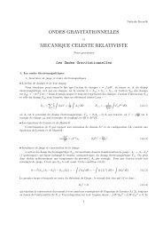
BBH Metric Analytic Approximation: Initial Data 

Buffer Zone (O ) 

34 

00000000000000000000000000000000000000000000000000 

11111111111111111111111111111111111111111111111111 

11111111111111111111111111111111111111111111111111 

00000000000000000000000000000000000000000000000000 

00000000000000000000000000000000000000000000000000 

11111111111111111111111111111111111111111111111111 

11111111111111111111111111111111111111111111111111 

00000000000000000000000000000000000000000000000000 

00000000000000000000000000000000000000000000000000 

11111111111111111111111111111111111111111111111111 

11111111111111111111111111111111111111111111111111 

3 

00000000000000000000000000000000000000000000000000 

Inner Zone BH 2 (C ) 

00000000000000000000000000000000000000000000000000 

11111111111111111111111111111111111111111111111111 

11111111111111111111111111111111111111111111111111 

00000000000000000000000000000000000000000000000000 

00000000000000000000000000000000000000000000000000 

11111111111111111111111111111111111111111111111111 

000000000 

00000000000000000000000000000000000000000000000000 

111111111 2 

11111111111111111111111111111111111111111111111111 

111111111 

13 

000000 

111111 

000000000 

11111111111111111111111111111111111111111111111111 

00000000000000000000000000000000000000000000000000 

00000000000000000000000000000000000000000000000000 

000000000 

111111111 

000000 

11111111111111111111111111111111111111111111111111 

111111 

111111111 

000000 

111111 

000000000 

11111111111111111111111111111111111111111111111111 

00000000000000000000000000000000000000000000000000 

00000000000000000000000000000000000000000000000000 

000000000 

111111111 

000000 

11111111111111111111111111111111111111111111111111 

111111 

111111111 

000000 

111111 

000000000 

11111111111111111111111111111111111111111111111111 

00000000000000000000000000000000000000000000000000 

Buffer 

Zone 

(O ) 

y 

Buffer 

Zone (O ) 

Far Zone (C ) 

4 

Inner Zone BH 1 (C ) 

BH 1 

00000000000000000000000000000000000000000000000000 

000000000 

111111111 

000000 

11111111111111111111111111111111111111111111111111 

111111 

111111111 

000000000 

11111111111111111111111111111111111111111111111111 

00000000000000000000000000000000000000000000000000 

00000000000000000000000000000000000000000000000000 

000000000 

11111111111111111111111111111111111111111111111111 

111111111 

1 

11111111111111111111111111111111111111111111111111 

00000000000000000000000000000000000000000000000000 

BH 2 

Near Zone (C ) 

00000000000000000000000000000000000000000000000000 

11111111111111111111111111111111111111111111111111 

11111111111111111111111111111111111111111111111111 

00000000000000000000000000000000000000000000000000 

00000000000000000000000000000000000000000000000000 

11111111111111111111111111111111111111111111111111 

11111111111111111111111111111111111111111111111111 

23 

00000000000000000000000000000000000000000000000000 

00000000000000000000000000000000000000000000000000 

11111111111111111111111111111111111111111111111111 

11111111111111111111111111111111111111111111111111 

00000000000000000000000000000000000000000000000000 

00000000000000000000000000000000000000000000000000 

11111111111111111111111111111111111111111111111111 

11111111111111111111111111111111111111111111111111 

00000000000000000000000000000000000000000000000000 

11111111111111111111111111111111111111111111111111 

00000000000000000000000000000000000000000000000000 

Bruno C. Mundim Magnetized Accretion onto Inspiraling BBH 2013-05-23 

b 

x

BBH Metric Analytic Approximation: Zones 

Zone rin rout 

Inner zone 1 (r1) 0 ≪ r12 

Inner zone 2 (r2) 0 ≪ r12 

Near zone (rA) ≫ mA ≪ λ 

Far zone (r) ≫ r12 ∞ 

r12: Orbital separation 

λ: GW wavelength 

Zone Region 

IZ-NZ buffer zone mA ≪ rA ≪ r12 

NZ-FZ buffer zone r12 ≪ r ≪ λ 

BZ(NZ-FZ) 

IZ2 

y 

NZ 

BZ(IZ2-NZ) 

r12 

IZ1 

BZ(IZ1-NZ) 


FZ 

x

BBH Metric Analytic Approximation: Inner Zone 

Inner Zone (IZ) 

(Non-spinning) BH + tidal 

perturbations 

gµν = g CS 

µν + hµν , 

Horizon penetrating 

coordinates: 

Cook and Scheel’s 

harmonic coordinates 

Parametrization: 

hµν = qµν(x i )Eµν(t) + kµν(x i )Bµν(t) , 

Tidal fields: Eµν and Bµν are 

elect. and mag. multipoles of 

the external universe’s Weyl 

BZ(NZ-FZ) 

IZ2 

y 

NZ 

BZ(IZ2-NZ) 

r12 

IZ1 

BZ(IZ1-NZ) 


FZ 

x

BBH Metric Analytic Approximation: Near Zone 

Near Zone (NZ) 

Flat + non-linear perturbation 

gµν = ηµν + hµν , 

post-Newtonian approach 

(slow motion, weak field) 

ηhµν ∝ Tµν(y i A) + τµν(h 2 ) , 

Harmonic coordinates 


htt = 2m1 

2 m1 + O , 

r1 

m1 

v 

r1 

2 , v 4 

 

, 

r 2 1 

BZ(NZ-FZ) 

IZ2 

y 

NZ 

BZ(IZ2-NZ) 

r12 

IZ1 

BZ(IZ1-NZ) 


FZ 

x

BBH Metric Analytic Approximation: Far Zone 

Far Zone (FZ) 

Flat + multipoles 

gµν = ηµν + hµν , 

post-Minkowskian theory 

(slow motion, weak field) 

Harmonic coordinates 

Time retardation u = t − r 

based on the flat-spacetime 

retarded Green function 


h tt 

1 

∝ ∂L 

r IL(u) 

 

, 

BZ(NZ-FZ) 

IZ2 

y 

NZ 

BZ(IZ2-NZ) 

r12 

IZ1 

BZ(IZ1-NZ) 


FZ 

x

BBH Metric Analytic Approximation: Buffer Zones 

Buffer Zone (BZ) 

Asymptotic matching and 

transition functions 

NZ-FZ (Same Coords.) 

Only transition functions. 

IZ-NZ (Different Coords.) 

Tidal fields and Coord. Trans. 

set in the matching 

BZ(NZ-FZ) 

IZ2 

y 

NZ 

BZ(IZ2-NZ) 

r12 

IZ1 

BZ(IZ1-NZ) 


FZ 

x

BBH Metric Analytic Approximation: Evolution 

Asymptotic matching fixes the coordinate transformation 

(perturbatively) and the tidal fields in the IZ. 

Problem: it assumes both BHs lie on x-axis at t = t0 for some inertial 

coordinate system. 

How to adapt this metric for evolution? 

Solution: rigid rotation of the spatial coordinates back and forth. 

The location of each hole in the NZ coordinates: 

x k i,NZ = {ri cos φ, ri sin φ, 0} 

Transform NZ and FZ metrics to a coordinates where the holes lie on 

the x-axis, match them to the IZ, and transform the full metric 

(IZ+NZ+FZ) back to the simulation inertial coordinates: 

x ′ NZ = xNZ cos φ + yNZ sin φ 

y ′ NZ = −xNZ sin φ + yNZ cos φ 


Error Analysis: Ricci Tensor and Ricci Scalar 

Christoffel symbols and derivatives: 

Γ ρ µν = 1 

2 g ρσ [gνσ,µ + gµσ,ν − gµν,σ] 

Ricci Tensor: 

Γ ρ 

µν,λ 

= 1 

2 g ρσ ,λ [gνσ,µ + gµσ,ν − gµν,σ] 

+ 1 

2 g ρσ [gνσ,µλ + gµσ,νλ − gµν,σλ] 

Rµρ = Γ ν µρ,ν − Γ ν νρ,µ + Γ α µρΓ ν αν − Γ α νρΓ ν αµ 

Ricci Scalar: R = R µ µ. 

In vacuum, an exact metric solution satisfies: 

Rµν = 0 and R = 0 

While our aproximate analytic metric has an error associated with it: 

Rµν = O(ɛ) and R = O(ɛ) 


Ricci Scalar 2nd Order Convergence 

Figure: (Left) L2-norm calculated over a simulation domain ranging from 

[−12, −12, −0.75] to [12, 12, 0.75] with a uniform mesh spacing following a 2 : 1 

ratio. (Right) Ricci l2-norm over the same volume for the coarsest mesh spacing, 

0.05M. Vertical dashed lines from left to right indicate separations of 14M, 12M, 

10M and 8M. 






Ricci Scalar: Evolution 


Ricci Scalar: Evolution 

Figure: Ricci scalar as a function of time from a separation of 20M to 8M on left 

panel (linear color scale). Absolute value of the Ricci scalar on the right panel 

(log color scale). Approximately 10 grid points across the horizon radius 

(rBH = 0.4875M). 


Ricci Scalar as a Function of Approximation Order 


Ricci Scalar as a Function of Approximation Order 


Circumbinary Disks 

Newtonian Hydrodynamic Simulations: 

BBH exerts torque on gas via its time-varying mass quadrupole 

moment. 

BBH torque restores some of the accreting gas’ angular momentum, 

thereby diminishing the mass accretion rate through the gas. 

Surface density tends to build-up at r ∼ 2a as matter accretes faster 

beyond gap. 

Newtonian MHD Simulations: 

MHD torques seem to be able to accrete more material through the 

gap, but gap still exists. 

GRMHD Simulations in the post-Newtonian Regime (our project): 

Can MHD torques keep the disk/gap near the binary? 

What is the mass distribution in the inner disk? It is crucial for 

accurate EM models as emissivity typically scales as ρ n 


Circumbinary Magnetized Disks: Simulation Setup 

Two simulations with initial binary separation of a0 = 20M: 

Secularly evolving run, RunSE: binary evolves at an artificially fixed 

separation for ∼ 75000M (or ∼ 140 orbits). 

Inspiral run, RunIn, binary starts at a RunSE snapshot, t = 40000M 

(or ∼ 100 orbits), to let the disk relax. It inspirals afterwards up to 

a 8M. 

2.5PN (NZ) metric; Domain: r = [0.75a0, 13a0] = [15M, 260M] 

Binary separation, a(t), and orbital phase, φ(t), up to 3.5PN. 


Circumbinary Magnetized Disks: Disk Initial Data 

Radiatively efficient, geometrically thin accretion disk: 

Disk extended over r = [3a0, 10a0]. 

Pressure maximum at rp = 5a0. 

Poloidal magnetic field following density contours. 

Near “equilibrim” disk solution using time averaged spacetime. 

Cool to constant entropy such that the disk aspect ratio is constant 

and H/r = 0.1 

Cooling function can be used as an emissivity in a GR ray-tracing code. 


Surface Density: Evolution 

Figure: Surface density time evolution (log 10 color scale) for RunIN (left) and 

RunSE (right). 

 

Σ(r, φ) ≡ 

dθ √ 

−gρ/ gφφ(θ = π/2); (1) 


Surface Density: Streams and Lump 

Figure: Color contours of surface density in log 10 (left) and linear (right) color 

scales, emphasizing the streams from the disk toward the binary members and the 

asymmetric density growth in the inner disk, respectively. 


Surface Density: Azimuthally Averaged 

Figure: Color contours of log 10 Σ(r) as a function of time for RunIN (left) and 

RunSE (right). The black dashed curve shows 2a(t). 



Figure: Color contours of log 10 Σ(r/a(t)) as a function of time for RunIN (left) 

and RunSE (right). 




Accretion Rate 

Figure: (Left) Accretion rate through the inner boundary: RunSE (black) and 

RunIN (gray). (Right) Time-averaged accretion rate during four equally spaced 

segments from t = 30, 000M (black) till the end of RunSE. 

Both RunIN and RunSE accretion rate decrease over time. 

Decrease due largely to torques. Decrease of RunIN also due to 

binary orbital decoupling. 


Luminosity Variability 

Figure: (r, t) spacetime (left) and luminosity integrated over radius (right). 









Figure: (r, ω) spacetime (left) and FPS of luminosity integrated over radius 

(right). 



Figure: (r, ω) spacetime (left) and FPS of luminosity integrated over radius 

(right). 


Luminosity Variability: Discussion 

Fourier power spectrum shows a strong, sharp peak at frequency 

ωpeak = 1.47Ωbin with rpeak 2.3a. 

and a weaker peak at the Ωlump = 0.26Ωbin, corresponding to the 

orbital frequency at the radius of the surface density maximum 

rlump 2.4a. 

We can identify ωpeak with the rate at which the lump approaches the 

orbital phase of a member of the binary: ωpeak = 2(Ωbin − Ωlump). 

When the lump draws close to one of the BHs, a new stream forms, 

falls inward, and it is split into two pieces. One of them gains angular 

momentum and sweeps back out to the disk, and shocks against the 

gas. 

It is this process that modulates the light curve. 


Conclusion and Future Work 

Demonstrated consistency with prior work in the Newtonian regime. 

Investigated the evolution of the disk with separation. 

A disk can follow the binary to very small separations, before 

decoupling. 

Measured the luminosity from a self-consistent cooling rate. 

Luminosity characteristic of AGN with excess at edge of gap due to 

dissipated binary torque work. 

Strong periodic signal found from the binary-lump interaction 

We need ray-trace in order to conclude if disk opacity will blur the 

signal. 

Need to calculate the dynamics in the vicinity of black holes 

How does the lump evolve after merger? 

Does the lump form with unequal mass or precessing binaries? 


Extra Slides 


Ricci Scalar: Evolution (Zoom Around a Black-Hole) 


Ricci Scalar: Evolution (Zoom Around a Black-Hole) 

Figure: Ricci scalar absolute value on a linear color scale around the “right” BH 

at t = 660M. The mesh spacing is 0.0125M (left) and 0.00625M (right) 

resulting into 39 and 78 grid points per horizon radius (rBH = 0.4875M). 


Ricci Scalar: Case for Higher Order Approximations. 

2nd order FDAs result in large computational effort to calculate the 

Ricci scalar to perturbative order accuracy, Rµν = O(ɛ). 

4th order approximation leads to faster convergence. 

For example, pick a point at the horizon, (0.0, 9.673556531, 0.3, 0.2), 

for an initial separation of 20M. The various quantities on the table 2 

below start to agree on the first significant figure only when 

dt = dx = dy = dz = h = 0.00625M, or 78 grid points per rBH. 

Note that a typical equal mass BHB simulation using full GR uses 

approximately 20 grid points per rAH on the finest AMR grid. 



2nd: 4th: 

Rtt = 0.01024587050684905 Rtt = 0.01007850127240062 

Rtx = 0.03228380078907006 Rtx = 0.0340889478274195 

Rty = −0.02308902839605859 Rty = −0.02298639795941293 

Rtz = −0.02006201110556877 Rtz = −0.02032786334618492 

Rxx = −0.6774182693609987 Rxx = −0.6650699268486431 

Rxy = 0.3413360547161979 Rxy = 0.3261324979719031 

Rxz = 0.348427534006535 Rxz = 0.3356062612167152 

Ryy = −0.1977530448946112 Ryy = −0.2060409626394311 

Ryz = −0.1865524325067573 Ryz = −0.1884958238515893 

Rzz = −0.2906179378901275 Rzz = −0.297516599915685 

R = −0.2657411795293186 R = −0.2698938651121096 

H = 0.01469997464077989 H = 0.0131591785513933 

M = 0.01504264551925634 M = 0.0167759321900986 

Table: Ricci tensor, scalar and constraints calculated using 2nd (left) and 4th 

(right) order FDA operators. 



h=0.0125: h=0.025: h=0.05: 

Rtt = 0.003196804677 0.01525931246 −0.7872097038 

Rtx = 0.06012934193 1.021136533 18.02810729 

Rty = −0.07799147144 −1.345320048 −22.01926661 

Rtz = 0.002133967513 0.01126266918 0.08158737450 

Rxx = 0.04656790023 0.7555766992 11.79503573 

Rxy = −0.006635370634 −0.1286574330 −1.910954363 

Rxz = 0.05114508275 0.8262931061 12.41963629 

Ryy = 0.3721293525 6.343315783 104.1051001 

Ryz = 0.07746675602 1.328459405 23.84528796 

Rzz = 0.05812650456 0.9723960616 16.50214637 

R = 0.08089705926 1.351036267 21.89512132 

H = −0.7001806355 −11.94584103 −195.1180949 

M = 0.1307027219 2.205683272 26.61166151 

Table: Percentile variation with respect to reference resolution, h = 0.00625M for 

4th order FDA. 39 (left), 20 (center) and 10 (right) grid points per rBH. 


Transition Function Effects 

Transition function used in the buffer zones: 

⎧ 

⎪⎨ 0 , r ≤ r0 , 

f = 1 

⎪⎩ 

2 (1 + tanh{(s/π)[χ − q2 /χ]}) , 

1 , 

r0 < r < r0 + w , 

r ≥ r0 + w , 

where χ = χ(r, r0, w) = tan[π(r − r0)/(2w)] and 

f = f (r, r0, w, q, s). 

Focus on the NZ-FZ buffer zone, since this region results into a large 

“bump” when higher order PN terms are used. 


(2)


Figure: Transition function for different values of parameters q and s as in 

f (r, r0, w, q, s). 



Figure: (Left) Comparison of the resummed O(v 5 ) Ricci Scalar between the NZ 

and FZ metrics. (Right) Resummed O(v 5 ) Ricci Scalar for different values of 

transition function parameters q and s as in f (r, r0, w, q, s). 



Figure: Resummed O(v 5 ) gxy IZ, NZ and FZ pieces (left) and gxy (right) for 

different values of transition function parameters q and s as in f (r, r0, w, q, s).

Magnetized Accretion onto Inspiraling Binary Black Holes - LUTH

Create successful ePaper yourself

Delete template?

Save as template?