Guide to Best Practices for Ocean CO2 Measurements - Aquatic ...
Guide to Best Practices for Ocean CO2 Measurements - Aquatic ...
Guide to Best Practices for Ocean CO2 Measurements - Aquatic ...

You also want an ePaper? Increase the reach of your titles
YUMPU automatically turns print PDFs into web optimized ePapers that Google loves.
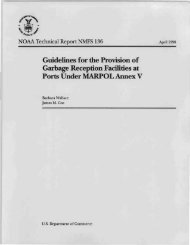
urette<br />
mL<br />
Metrohm Dosimat<br />
probe<br />
<strong>to</strong> digital<br />
thermometer<br />
In from<br />
thermostat bath<br />
HCl/NaCl<br />
titrant<br />
thermometer<br />
probe<br />
combination electrode<br />
STIR<br />
<strong>to</strong> e.m.f.<br />
measuring<br />
system<br />
out <strong>to</strong><br />
thermostat<br />
bath<br />
This <strong>Guide</strong> contains the most up-<strong>to</strong>-date in<strong>for</strong>mation available on the<br />
chemistry of CO 2 in sea water and the methodology of determining<br />
carbon system parameters, and is an attempt <strong>to</strong> serve as a clear and<br />
unambiguous set of instructions <strong>to</strong> investiga<strong>to</strong>rs who are setting up <strong>to</strong><br />
analyze these parameters in sea water.<br />
North Pacific Marine Science Organization<br />
<strong>Guide</strong> <strong>to</strong> <strong>Best</strong> <strong>Practices</strong> <strong>for</strong> <strong>Ocean</strong> C0 2 Measurments 2007 PICES SPECIAL PUBLICATION<br />
3<br />
<strong>Guide</strong> <strong>to</strong> <strong>Best</strong> <strong>Practices</strong> <strong>for</strong><br />
<strong>Ocean</strong> CO 2 <strong>Measurements</strong><br />
P I C E S S P E C I A L P U B L I C AT I O N 3<br />
IOCCP REPORT No. 8
Chapter 1 — Introduction<br />
Chapter 1<br />
Introduction <strong>to</strong> the <strong>Guide</strong><br />
The collection of extensive, reliable, oceanic carbon data was a key component<br />
of the Joint Global <strong>Ocean</strong> Flux Study (JGOFS) and World <strong>Ocean</strong> Circulation<br />
Experiment (WOCE) and continues <strong>to</strong> be a corners<strong>to</strong>ne of the global climate<br />
research ef<strong>for</strong>t. This <strong>Guide</strong> was originally prepared at the request, and with the<br />
active participation, of a science team <strong>for</strong>med by the U.S. Department of Energy<br />
(DOE) <strong>to</strong> carry out the first global survey of carbon dioxide in the oceans (DOE.<br />
1994. Handbook of methods <strong>for</strong> the analysis of the various parameters of the<br />
carbon dioxide system in sea water; version 2, A.G. Dickson and C. Goyet, Eds.<br />
ORNL/CDIAC-74). The manual has been updated several times since, and the<br />
current version contains the most up-<strong>to</strong>-date in<strong>for</strong>mation available on the<br />
chemistry of <strong>CO2</strong> in sea water and the methodology of determining carbon<br />
system parameters. This revision has been made possible by the generous<br />
support of the North Pacific Marine Science Organization (PICES), the<br />
International <strong>Ocean</strong> Carbon Coordination Project (IOCCP) co-sponsored by the<br />
Scientific Committee on <strong>Ocean</strong> Research (SCOR) and the Intergovernmental<br />
<strong>Ocean</strong>ographic Commission (IOC) of UNESCO, and the Carbon Dioxide<br />
In<strong>for</strong>mation Analysis Center (CDIAC). The edi<strong>to</strong>rs are extremely grateful <strong>to</strong><br />
Alex Kozyr and Mikhail Krassovski at CDIAC <strong>for</strong> their hard work in helping us<br />
<strong>to</strong> complete this revised volume. This manual should be cited as Dickson, A.G.,<br />
Sabine, C.L. and Christian, J.R. (Eds.) 2007. <strong>Guide</strong> <strong>to</strong> best practices <strong>for</strong> ocean<br />
<strong>CO2</strong> measurements. PICES Special Publication 3, 191 pp.<br />
The procedures detailed in the following pages have been subjected <strong>to</strong> open<br />
review by the ocean carbon science community and describe well-tested<br />
methods. They are intended <strong>to</strong> provide standard operating procedures (SOPs),<br />
<strong>to</strong>gether with an appropriate quality control plan. These are not the only<br />
measurement techniques in use <strong>for</strong> the parameters of the oceanic carbon system;<br />
however, they do represent the current state-of-the-art <strong>for</strong> shipboard<br />
measurements. In the end, we hope that this manual can serve as a clear and<br />
unambiguous guide <strong>to</strong> other investiga<strong>to</strong>rs who are setting up <strong>to</strong> analyze the<br />
various parameters of the carbon dioxide system in sea water. We envision it as<br />
an evolving document, updated where necessary. The edi<strong>to</strong>rs welcome comments<br />
and suggestions <strong>for</strong> use in preparing future revisions. The procedures included<br />
Page 1 of 2
Chapter 1 — Introduction<br />
here are not simply descriptions of a particular method in current use in a single<br />
labora<strong>to</strong>ry, but rather provide standard operating procedures which have been<br />
written in a fashion that will—we trust—allow anyone <strong>to</strong> implement the method<br />
successfully. In some cases there is no consensus about the best approach; these<br />
areas are identified in the footnotes <strong>to</strong> the various procedures along with other<br />
hints and tips.<br />
In addition <strong>to</strong> the written procedures, general in<strong>for</strong>mation about the solution<br />
chemistry of the carbon dioxide system in sea water has been provided<br />
(Chapter 2) <strong>to</strong>gether with recommended values <strong>for</strong> the physical and<br />
thermodynamic data needed <strong>for</strong> certain computations (Chapter 5). This<br />
in<strong>for</strong>mation is needed <strong>to</strong> understand certain aspects of the procedures, and users<br />
of this <strong>Guide</strong> are advised <strong>to</strong> study Chapter 2 carefully. The user is cautioned that<br />
equilibrium constants employed in ocean carbon chemistry have specific values<br />
<strong>for</strong> different pH scales, and values in the published literature may be on different<br />
scales than the one used here; it is very important <strong>to</strong> make sure that all constants<br />
used in a particular calculation are on the same scale. General advice about<br />
appropriate quality control measures has also been included (Chapter 3). The<br />
SOPs (Chapter 4) are numbered. Numbers less than 10 are reserved <strong>for</strong><br />
procedures describing sampling and analysis, numbers 11–20 <strong>for</strong> procedures <strong>for</strong><br />
calibration, etc., and numbers 21 and upward <strong>for</strong> procedures <strong>for</strong> computations<br />
and quality control. This scheme allows <strong>for</strong> the addition of further SOPs in the<br />
future. Each of the procedures has been marked with a date of last revision and a<br />
version number. When citing a particular SOP in a report or technical paper, we<br />
recommend stating the version number of the procedure used. We envision this<br />
<strong>Guide</strong> being further expanded and updated in the future; thus the version number<br />
identifies unambiguously the exact procedure that is being referred <strong>to</strong>. Any errors<br />
in the text or corrections that arise as the methods evolve can be reported <strong>to</strong> Alex<br />
Kozyr at CDIAC (kozyra@ornl.gov).<br />
Page 2 of 2<br />
Andrew G. Dickson, Chris<strong>to</strong>pher L. Sabine, and James R. Christian<br />
Edi<strong>to</strong>rs
Chapter 2 — Solution chemistry Oc<strong>to</strong>ber 12, 2007<br />
Chapter 2<br />
Solution chemistry of<br />
carbon dioxide in sea water<br />
1. Introduction<br />
This chapter outlines the chemistry of carbon dioxide in sea water so as <strong>to</strong><br />
provide a coherent background <strong>for</strong> the rest of this <strong>Guide</strong>. The following sections<br />
lay out the thermodynamic framework required <strong>for</strong> an understanding of the<br />
solution chemistry; the thermodynamic data needed <strong>to</strong> interpret field and<br />
labora<strong>to</strong>ry results are presented in Chapter 5.<br />
2. Reactions in solution<br />
The reactions that take place when carbon dioxide dissolves in water can be<br />
represented by the following series of equilibria:<br />
CO 2(g) CO 2(aq)<br />
, (1)<br />
CO 2(aq) + H2O(l) H2CO 3(aq)<br />
, (2)<br />
H CO (aq) H (aq) + HCO (aq) , (3)<br />
+ –<br />
2 3 3<br />
– + 2–<br />
HCO 3(aq) H (aq) + CO 3 (aq) ; (4)<br />
the notations (g), (l), (aq) refer <strong>to</strong> the state of the species, i.e., a gas, a liquid or in<br />
aqueous solution respectively. It is difficult <strong>to</strong> analytically distinguish between<br />
the species <strong>CO2</strong>(aq) and H2CO3(aq). It is usual <strong>to</strong> combine the concentrations of<br />
<strong>CO2</strong>(aq) and H2CO3(aq) and <strong>to</strong> express this sum as the concentration of a<br />
hypothetical species, CO* (aq) . 2<br />
Redefining (1), (2), and (3) in terms of this species gives<br />
CO (g) CO (aq)<br />
(5)<br />
*<br />
2 2<br />
*<br />
2 + 2<br />
+ + –<br />
3<br />
CO (aq) H O(l) H (aq) HCO (aq)<br />
(6)<br />
Page 1 of 13
Oc<strong>to</strong>ber 12, 2007 Chapter 2 — Solution chemistry<br />
The equilibrium relationships between the concentrations of these various species<br />
can then be written as<br />
Page 2 of 13<br />
K = [CO ] f(CO<br />
) , (7)<br />
0<br />
*<br />
2 2<br />
+ – *<br />
1 3 2<br />
K = [H ][HCO ] [CO ] , (8)<br />
K = [H ][CO ] [HCO ] . (9)<br />
+ 2– –<br />
2 3 3<br />
In these equations, ƒ(<strong>CO2</strong>) is the fugacity of carbon dioxide in the gas phase and<br />
brackets represent <strong>to</strong>tal s<strong>to</strong>ichiometric concentrations 1 of the particular chemical<br />
species enclosed. These equilibrium constants are functions of the temperature,<br />
pressure and salinity of the solution (e.g., sea water) and have been measured in a<br />
variety of studies (see Chapter 5).<br />
3. Fugacity<br />
The fugacity of carbon dioxide is not the same as its partial pressure—the<br />
product of mole fraction and <strong>to</strong>tal pressure, x(<strong>CO2</strong>)⋅p—but rather takes account<br />
of the non-ideal nature of the gas phase. The fugacity of a gas such as <strong>CO2</strong> can<br />
be determined from knowledge of its equation of state:<br />
p ⎛ 1<br />
⎞<br />
f(CO 2) = x(CO 2) ⋅ p⋅exp ⎜ ( V(CO 2)<br />
RT / p′ ) dp′<br />
⎜<br />
− ⎟<br />
RT ∫ ⎟<br />
. (10)<br />
⎝ 0<br />
⎠<br />
The equation of state of a real gas such as <strong>CO2</strong>, either alone or in a mixture, can<br />
be represented by a virial expression:<br />
pV(CO 2)<br />
B( x, T) C( x, T)<br />
= 1 + + + . . .<br />
(11)<br />
2<br />
RT V (CO ) V (CO )<br />
2 2<br />
This equation, truncated after the second term, is usually adequate <strong>to</strong> represent<br />
p–V–T properties at pressures up <strong>to</strong> a few atmospheres (Dymond and Smith,<br />
1980).<br />
It is known from statistical mechanics that the virial coefficients B(x, T), C(x, T),<br />
etc. relate <strong>to</strong> pair-wise interactions in the gas phase (Guggenheim, 1967). This<br />
property can be used <strong>to</strong> estimate B(x, T) <strong>for</strong> particular gas mixtures, such as <strong>CO2</strong><br />
in air, from measurements on binary mixtures or from a model of the<br />
intermolecular potential energy function <strong>for</strong> the molecules concerned. The<br />
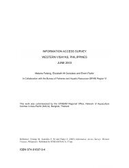
magnitude of the fugacity coefficient (the ratio of fugacity <strong>to</strong> partial pressure) is a<br />
function both of temperature and of gas phase composition (Fig. 1).<br />
1 Strictly, equations (7) <strong>to</strong> (9) should be expressed in terms of activities rather than<br />
concentrations. However, as the activity coefficients are approximately constant <strong>for</strong><br />
small amounts of reacting species in a background medium, these expressions are valid<br />
and correspond <strong>to</strong> “ionic medium” equilibrium constants based on a sea water medium.
Chapter 2 — Solution chemistry Oc<strong>to</strong>ber 12, 2007<br />
Fig. 1 Variation of the fugacity coefficient with temperature at 1 atm <strong>to</strong>tal pressure <strong>for</strong><br />
pure <strong>CO2</strong> gas and <strong>for</strong> <strong>CO2</strong> in air: x(<strong>CO2</strong>) = 350 × 10 –6 (calculated using the procedure<br />
described in SOP 24 of this <strong>Guide</strong>).<br />
4. Analytical parameters of the <strong>CO2</strong> system<br />
Un<strong>for</strong>tunately, the concentrations of the individual species of the carbon dioxide<br />
system in solution can not be measured directly. There are, however, four<br />
parameters that can be measured. These are used <strong>to</strong>gether with ancillary<br />
in<strong>for</strong>mation <strong>to</strong> obtain a complete description of the carbon dioxide system in sea<br />
water. Methods <strong>for</strong> determining each of these parameters are detailed in<br />
Chapter 4.<br />
4.1 Total dissolved inorganic carbon<br />
The <strong>to</strong>tal dissolved inorganic carbon in a sea water sample:<br />
C = [CO ] + [HCO ] + [CO ]<br />
(12)<br />
* – 2–<br />
T 2 3 3<br />
can be measured directly by acidifying the sample, extracting the <strong>CO2</strong> gas that is<br />
produced and measuring its amount.<br />
4.2 Total alkalinity<br />
The <strong>to</strong>tal alkalinity of a sample of sea water is a <strong>for</strong>m of mass-conservation<br />
relationship <strong>for</strong> hydrogen ion. It is rigorously defined (Dickson, 1981) as “. . . the<br />
number of moles of hydrogen ion equivalent <strong>to</strong> the excess of pro<strong>to</strong>n accep<strong>to</strong>rs<br />
(bases <strong>for</strong>med from weak acids with a dissociation constant K ≤ 10 –4.5 at 25°C<br />
and zero ionic strength) over pro<strong>to</strong>n donors (acids with K > 10 –4.5 ) in 1 kilogram<br />
of sample.” Thus<br />
− 2− − − 2−<br />
AT<br />
= [HCO 3] + 2[CO 3 ] + [B(OH) 4] + [OH ] + [HPO 4 ]<br />
3−<br />
− −<br />
+ 2[PO 4 ] + [SiO(OH) 3] + [NH 3]<br />
+ [HS ] + ...<br />
+ −<br />
−[H ] −[HSO ] −[HF] −[HPO ] − ...<br />
(13)<br />
F 4 3 4<br />
Page 3 of 13
Oc<strong>to</strong>ber 12, 2007 Chapter 2 — Solution chemistry<br />
where the ellipses stand <strong>for</strong> additional minor acid or base species that are either<br />
unidentified or present in such small amounts that they can be safely neglected.<br />
[H + ]F is the free concentration of hydrogen ion—see equation (15).<br />
4.3 Fugacity of <strong>CO2</strong> in equilibrium with a sea water sample<br />
This measurement typically requires a gas phase that is in equilibrium with a sea<br />
water sample at a known pressure and temperature. The concentration of <strong>CO2</strong> is<br />
then determined in the gas phase and the corresponding value of ƒ(<strong>CO2</strong>)—<strong>for</strong><br />
that temperature—estimated from equation (10).<br />
4.4 Total hydrogen ion concentration<br />
The hydrogen ion concentration in sea water is usually reported as pH:<br />
+<br />
pH =− log[H ].<br />
(14)<br />
Although the concept of a <strong>to</strong>tal hydrogen ion concentration is somewhat<br />
confusing 2 , it is needed <strong>to</strong> define acid dissociation constants accurately in sea<br />
water (Dickson, 1990). Total hydrogen ion concentration is defined as<br />
+ +<br />
F T S<br />
[H + ]F is the free hydrogen ion concentration, ST is the <strong>to</strong>tal sulfate concentration<br />
2– –<br />
–<br />
( [SO 4 ] + [HSO 4]<br />
) and KS is the acid dissociation constant <strong>for</strong> HSO 4 . At pH<br />
values above 4, equation (15) can be approximated as<br />
Page 4 of 13<br />
[H ] = [H ] ⋅ (1 + S / K ) . (15)<br />
+ +<br />
[H ] = [H ] + [HSO ] . (16)<br />
–<br />
F 4<br />
The various equilibrium constants required <strong>to</strong> describe acid–base chemistry in<br />
sea water have been measured in the labora<strong>to</strong>ry (see Chapter 5 <strong>for</strong> recommended<br />
constants). In addition <strong>to</strong> knowing the carbon parameters, the <strong>to</strong>tal<br />
concentrations of the various other (non-<strong>CO2</strong>) acid–base systems in the sample of<br />
interest are needed <strong>to</strong> fully constrain the carbon dioxide system in sea water. The<br />
<strong>to</strong>tal concentrations of conservative constituents, such as borate, sulfate, and<br />
fluoride, can be estimated from salinity. Those of non-conservative constituents,<br />
such as phosphate, silicate, ammonia or hydrogen sulfide, must be measured but<br />
approximate “reference” concentrations are adequate <strong>for</strong> most purposes. Because<br />
of the relative consistency of the chemical constituents of sea water, it is<br />
generally accepted that only two of the four measurable carbon parameters are<br />
needed <strong>to</strong>gether with the equilibrium constants, temperature, pressure, and<br />
salinity, <strong>to</strong> have a complete description of the system (see Park (1969), Skirrow<br />
(1975), and the Annexe <strong>to</strong> this chapter).<br />
This practice assumes that our present knowledge of the nature, <strong>to</strong>tal<br />
concentrations, and thermodynamic properties of all the possible acid–base<br />
species in sea water is complete. It is probably better at this stage <strong>to</strong> overdetermine<br />
the system whenever possible, i.e., <strong>to</strong> measure more than two of these<br />
parameters on any given sample and <strong>to</strong> use the redundancy <strong>to</strong> confirm that the<br />
measurements fit with our understanding of the thermodynamics of acid–base<br />
processes in sea water.<br />
2<br />
See Dickson (1984, 1993) <strong>for</strong> a detailed discussion of the various pH scales that have<br />
been used in sea water.
5. Bibliography<br />
Chapter 2 — Solution chemistry Oc<strong>to</strong>ber 12, 2007<br />
Dickson, A.G. 1981. An exact definition of <strong>to</strong>tal alkalinity and a procedure <strong>for</strong> the<br />
estimation of alkalinity and <strong>to</strong>tal inorganic carbon from titration data. Deep-Sea Res.<br />
28A: 609–623.<br />
Dickson, A.G. 1984. pH scales and pro<strong>to</strong>n-transfer reactions in saline media such as sea<br />
water. Geochim. Cosmochim. Acta 48: 2299–2308.<br />
Dickson, A.G. 1990. Standard potential of the reaction: AgCl(s) + ½H2(g) = Ag(s) +<br />
HCl(aq), and the standard acidity constant of the ion HSO4 – in synthetic sea water<br />
from 273.15 <strong>to</strong> 318.15 K. J. Chem. Thermodyn. 22: 113–127.<br />
Dickson, A.G. 1993. The measurement of sea water pH. Mar. Chem. 44: 131–142.<br />
Dymond, J.H. and Smith, E.B. 1980. The Virial Coefficients of Pure Gases and Mixtures:<br />
A Critical Compilation. Clarendon Press, 518 pp.<br />
Guggenheim, E.A. 1967. Thermodynamics. An Advanced Treatment <strong>for</strong> Chemists and<br />
Physicists, 5th edition, North-Holland, 390 pp.<br />
Park, K. 1969. <strong>Ocean</strong>ic <strong>CO2</strong> system: an evaluation of ten methods of investigation.<br />
Limnol. <strong>Ocean</strong>ogr. 14: 179–186.<br />
Skirrow, G. 1975. The dissolved gases—carbon dioxide. In: Chemical <strong>Ocean</strong>ography,<br />
Vol. 2. Edited by J.P. Riley and G. Skirrow, Academic Press, London, pp. 1–192.<br />
Page 5 of 13
Oc<strong>to</strong>ber 12, 2007 Chapter 2 — Solution chemistry<br />
Annexe<br />
Equations that describe the <strong>CO2</strong> system in<br />
sea water<br />
It is possible, in theory, <strong>to</strong> obtain a complete description of the carbon dioxide<br />
system in a sample of sea water at a particular temperature and pressure provided<br />
that the following in<strong>for</strong>mation is known 3 :<br />
• the solubility constant <strong>for</strong> <strong>CO2</strong> in sea water, K0,<br />
• the equilibrium constants <strong>for</strong> each of the acid–base pairs that are assumed <strong>to</strong><br />
exist in the solution,<br />
• the <strong>to</strong>tal concentrations of all the non-<strong>CO2</strong> acid–base pairs,<br />
• the values of at least two of the <strong>CO2</strong> related parameters: CT , AT , f(<strong>CO2</strong>), [H + ].<br />
The optimal choice of experimental variables is dictated by the nature of the<br />
problem being studied and remains at the discretion of the investiga<strong>to</strong>r.<br />
Although each of the <strong>CO2</strong> related parameters is linearly independent, they are not<br />
orthogonal. For certain combinations there are limits <strong>to</strong> the accuracy with which<br />
the other parameters can be predicted from the measured data. These errors end<br />
up being propagated through the equations presented here. Such errors result<br />
from all the experimentally derived in<strong>for</strong>mation, including the various<br />
equilibrium constants. As a consequence it is usually better <strong>to</strong> measure a<br />
particular parameter directly using one of the methods detailed in Chapter 4 than<br />
<strong>to</strong> calculate it from other measurements.<br />
When more than two of the <strong>CO2</strong>-related parameters have been measured on a<br />
single sea water sample, it is possible <strong>to</strong> use the various possible pairs of<br />
parameters <strong>to</strong> compute the other redundant parameters and thus <strong>to</strong> assess the<br />
internal consistency of our knowledge of the system. Again, it is necessary <strong>to</strong><br />
take all the sources of error in<strong>to</strong> account when doing this. Alternately, one can<br />
describe the system independently of one or more of the dissociation constants<br />
<strong>for</strong> carbonic acid. Equations that allow each of these possibilities <strong>to</strong> be realized<br />
are derived here.<br />
3 The rank of the system of equilibrium equations that describes the acid–base chemistry<br />
of sea water—i.e., the number of linearly independent variables—is equal <strong>to</strong> the<br />
number of independent mass-conservation relationships plus the number of acid–base<br />
pairs considered (the number of dissociation constants).<br />
Page 6 of 13
Chapter 2 — Solution chemistry Oc<strong>to</strong>ber 12, 2007<br />
Table 1 Equations <strong>for</strong> the sea water acid–base system.<br />
Mass-conservation equations 4<br />
Equilibrium constants<br />
* – 2–<br />
C T = [CO 2] + [HCO 3] + [CO 3 ]<br />
(17)<br />
2 = [HCO ] + 2[CO 2<br />
] + [B(OH) ] + [OH ] + [HPO ]<br />
3−<br />
− −<br />
+ 2[PO 4 ] + [SiO(OH) 3] + [NH 3]<br />
+ [HS ] + ...<br />
+ −[H ] − −[HSO ] −[HF] −[HPO ] − ... (18)<br />
− − − − −<br />
AT 3 3 4 4<br />
F 4 3 4<br />
B = [B(OH) ] + [B(OH) ]<br />
(19)<br />
T 3<br />
–<br />
4<br />
S = [HSO ] + [SO ]<br />
(20)<br />
– 2–<br />
T 4 4<br />
–<br />
F T = [HF] + [F ]<br />
(21)<br />
P = [H PO ] + [H PO ] + [HPO ] + [PO ]<br />
(22)<br />
– 2– 3–<br />
T 3 4 2 4 4 4<br />
Si = [Si(OH) ] + [SiO(OH) ]<br />
(23)<br />
T 4<br />
–<br />
3<br />
NH<br />
= [NH ] + [NH ]<br />
(24)<br />
3T<br />
+<br />
4 3<br />
HS = + (25)<br />
–<br />
2 T [H2S] [HS ]<br />
K = [CO ] f(CO<br />
)<br />
(26)<br />
0<br />
*<br />
2 2<br />
K = [H ][HCO ] [CO ]<br />
(27)<br />
+ – *<br />
1 3 2<br />
K = [H ][CO ] [HCO ]<br />
(28)<br />
+ 2– –<br />
2 3 3<br />
K = [H ][B(OH) ] [B(OH) ]<br />
(29)<br />
+ –<br />
B 4 3<br />
W<br />
– [H ][OH ]<br />
K +<br />
= (30)<br />
K = [H ][SO ] [HSO ]<br />
(31)<br />
+ 2– –<br />
S 4 4<br />
F<br />
+ – [H ][F ] [HF]<br />
K = (32)<br />
K = [H ][H PO ] [H PO ]<br />
(33)<br />
+ –<br />
1P 2 4 3 4<br />
K = [H ][HPO ] [H PO ]<br />
(34)<br />
+ 2– –<br />
2P 4 2 4<br />
K = [H ][PO ] [HPO ]<br />
(35)<br />
+ 3– 2–<br />
3P 4 4<br />
K = [H ][SiO(OH) ] [Si(OH) ]<br />
(36)<br />
+ –<br />
Si 3 4<br />
K<br />
= [H ][NH ] [NH ]<br />
(37)<br />
+<br />
+<br />
NH3 3 4<br />
K = [H ][HS ] [H S]<br />
(38)<br />
+ –<br />
HS 2<br />
2<br />
4 The aqueous chemistry of Si is rather complex, and encompasses more species than are<br />
considered here. This approximation is adequate <strong>for</strong> the present purpose of estimating<br />
the silicate contribution <strong>to</strong> alkalinity.<br />
Page 7 of 13
Oc<strong>to</strong>ber 12, 2007 Chapter 2 — Solution chemistry<br />
Table 2 Expressions <strong>for</strong> the concentrations of the various species in equation (18).<br />
[H + ] and AT<br />
Page 8 of 13<br />
[HCO ]<br />
[CO ] =<br />
CK[H<br />
]<br />
+<br />
–<br />
T 1<br />
3 =<br />
+ 2<br />
+<br />
[H ] + K1[H ] + K1K2 CKK<br />
2–<br />
T 1 2<br />
3 + 2<br />
+<br />
[H ] + K1[H ] + K1K2 –<br />
4 BT + KB<br />
(39)<br />
(40)<br />
[B(OH) ] = (1 + [H ]/ )<br />
(41)<br />
[OH ] = K [H ]<br />
(42)<br />
– +<br />
3 4<br />
W<br />
+ 3 PT<br />
[H ]<br />
=<br />
+ 3 + 2 +<br />
[H ] + K1P[H ] + K1PK2P[H ] + K1PK2PK3P [H PO ]<br />
[H ]<br />
+ 2<br />
–<br />
T 1P<br />
2 4 =<br />
+ 3 + 2 +<br />
[H ] + K1P[H ] + K1PK2P[H ] + K1PK2PK3P [H PO ]<br />
[HPO ]<br />
[PO ] =<br />
PK<br />
+<br />
PK 2–<br />
T 1PK2P[H ]<br />
4 =<br />
+ 3 + 2 +<br />
[H ] + K1P[H ] + K1PK2P[H ] + K1PK2PK3P PK K K<br />
3–<br />
T 1P 2P 3P<br />
4 + 3 + 2 +<br />
[H ] + K1P[H ] + K1PK2P[H ] + K1PK2PK3P – [SiO(OH) 3] SiT (1 + [H ]/ KSi)<br />
(43)<br />
(44)<br />
(45)<br />
(46)<br />
= + (47)<br />
[NH ] = NH (1 + [H ]/ K )<br />
(48)<br />
+<br />
3 3T NH3<br />
[HS ] = HS (1 + [H ]/ K )<br />
(49)<br />
– +<br />
2 T H2S [H ] = [H ] (1 + S / K )<br />
(50)<br />
+ +<br />
F T S<br />
+<br />
[HSO ] = S (1 + K /[H ] )<br />
(51)<br />
–<br />
4 T S F<br />
+<br />
[HF] = F (1 + K /[H ])<br />
(52)<br />
T F<br />
The carbonate alkalinity (i.e., the contribution of carbonate species <strong>to</strong> the <strong>to</strong>tal<br />
alkalinity) is defined as<br />
− 2−<br />
AC 3 3<br />
= [HCO ] + 2[CO ] . (53)<br />
The concentrations of the non-<strong>CO2</strong> species that contribute <strong>to</strong> AT are calculated<br />
using the expressions given in Table 2, thus<br />
(<br />
− − − −<br />
A = A − [B(OH) ] + [OH ] + [HPO ] + 2[PO ]<br />
2 3<br />
C T 4 4 4<br />
− −<br />
+ [SiO(OH) 3] + [NH 3]<br />
+ [HS ] + ...<br />
+ −<br />
F 4 3 4<br />
− [H ] −[HSO ] −[HF] −[HPO ] − ...<br />
(54)<br />
)
Chapter 2 — Solution chemistry Oc<strong>to</strong>ber 12, 2007<br />
Then from (27),<br />
* [CO 2] K<br />
−<br />
1<br />
[HCO 3 ] = ,<br />
+ [H ]<br />
(55)<br />
and from (28),<br />
* [CO 2] K 2<br />
1 K<br />
− ⎛ ⎞ 2<br />
[CO 3 ] = ⎜ + + [H ]<br />
⎟ .<br />
⎝ ⎠[H<br />
]<br />
Substituting in<strong>to</strong> (53) and rearranging,<br />
(56)<br />
+ 2 A<br />
*<br />
C[H<br />
]<br />
[CO 2 ] =<br />
,<br />
+ K1([H ] + 2 K2)<br />
and hence<br />
(57)<br />
+ AC[H<br />
]<br />
− [HCO 3 ] =<br />
+ [H ] + 2K<br />
, (58)<br />
AK<br />
2−<br />
C 2<br />
[CO 3 ] =<br />
+ [H ] + 2K<br />
CT is calculated from (17) and f(<strong>CO2</strong>) from (26):<br />
[H + ] and ƒ(<strong>CO2</strong>)<br />
* [CO 2]is<br />
given by (26):<br />
Thus, from (27) and (28),<br />
0<br />
2<br />
2<br />
. (59)<br />
* [CO 2]<br />
f (CO 2)<br />
= . (60)<br />
K<br />
[CO ] = K f(CO<br />
) . (61)<br />
*<br />
2 0 2<br />
KKf 0 1 (CO 2)<br />
− [HCO 3 ]=<br />
, (62)<br />
+ [H ]<br />
KKK 2 0 1 2f(CO 2)<br />
− [CO 3 ] = . (63)<br />
+ 2 [H ]<br />
− 2−<br />
CT is calculated from (17) and AT from (18); [HCO 3 ] and [CO 3 ] are given by<br />
(62) and (63), the remaining terms are calculated from the expressions given in<br />
Table 2.<br />
[H + ] and CT<br />
Equations (27) and (28) are rearranged and substituted in<strong>to</strong> (17) <strong>to</strong> give<br />
⎛ K K K ⎞<br />
= [CO ] ⎜1+ +<br />
[H ] [H ]<br />
⎟.<br />
(64)<br />
⎝ ⎠<br />
*<br />
1 1 2<br />
C T 2 + + 2<br />
Page 9 of 13
Oc<strong>to</strong>ber 12, 2007 Chapter 2 — Solution chemistry<br />
Thus<br />
Page 10 of 13<br />
[CO ]<br />
[HCO ]<br />
C<br />
[H ]<br />
+ 2<br />
*<br />
T<br />
2 =<br />
+ 2<br />
+<br />
[H ] + K1[H ] + K1K2 [CO ] =<br />
CK[H<br />
]<br />
+<br />
–<br />
T 1<br />
3 =<br />
+ 2<br />
+<br />
[H ] + K1[H ] + K1K2 CKK<br />
2−<br />
T 1 2<br />
3 + 2<br />
+<br />
[H ] + K1[H ] + K1K2 , (65)<br />
, (66)<br />
. (67)<br />
f (CO 2 ) is calculated from (60) and AT from (18); the various terms needed are<br />
calculated from the expressions given in Table 2.<br />
AT and CT<br />
The easiest approach <strong>to</strong> using this pair of parameters is <strong>to</strong> rewrite (18), the<br />
expression <strong>for</strong> AT, in terms of <strong>to</strong>tal concentrations and [H + ] (see Table 2). The<br />
resulting equation is solved <strong>for</strong> [H + ] using either a New<strong>to</strong>n–Raphson technique or<br />
a simple iterative approach; a suitable initial estimate <strong>for</strong> calculations involving<br />
sea water is: [H + ] = 10 –8 mol kg –1 .<br />
Once [H + ] has been calculated,<br />
[HCO ]<br />
[CO ] =<br />
* [CO 2]is<br />
then calculated from<br />
and f (CO ) is calculated from (60).<br />
2<br />
AT and ƒ(<strong>CO2</strong>)<br />
* [CO 2]<br />
is given by (26):<br />
CK[H<br />
]<br />
+<br />
–<br />
T 1<br />
3 =<br />
+ 2<br />
+<br />
[H ] + K1[H ] + K1K2 CKK<br />
2−<br />
T 1 2<br />
3 + 2<br />
+<br />
[H ] + K1[H ] + K1K2 1<br />
, (68)<br />
. (69)<br />
+ − [H ][HCO *<br />
3 ]<br />
[CO 2]<br />
= (70)<br />
K<br />
[CO ] = K f(CO<br />
) . (71)<br />
*<br />
2 0 2<br />
Equations (27) and (28) are then rewritten as<br />
KKf 0 1 (CO 2)<br />
− [HCO 3 ]=<br />
, (72)<br />
+ [H ]<br />
KKK 2 0 1 2f(CO 2)<br />
− [CO 3 ] = . (73)<br />
+ 2 [H ]
Chapter 2 — Solution chemistry Oc<strong>to</strong>ber 12, 2007<br />
These terms are substituted in<strong>to</strong> (18) <strong>to</strong>gether with the remaining terms from<br />
Table 2. The resulting expression is solved <strong>for</strong> [H + ] using either a New<strong>to</strong>n–<br />
Raphson technique or a simple iterative approach; a suitable initial estimate <strong>for</strong><br />
ocean water is: [H + ] = 10 –8 mol kg –1 . Once [H + ] has been calculated, CT is<br />
− 2−<br />
calculated from (17) using the final values obtained <strong>for</strong> [HCO 3 ] and[CO 3 ] .<br />
CT and ƒ(<strong>CO2</strong>)<br />
For this calculation, it is convenient <strong>to</strong> define the constant<br />
For the equilibrium process,<br />
* [CO 2]<br />
is given by (26):<br />
[HCO ]<br />
K = K K = . (74)<br />
[CO ][CO ]<br />
− 2<br />
1/ 2 *<br />
3<br />
2−<br />
2 3<br />
CO (aq) + CO (aq) + H O(l) = 2HCO . (75)<br />
* 2−<br />
−<br />
2 3 2 3<br />
[CO ] = K f(CO<br />
)<br />
(76)<br />
*<br />
2 0 2<br />
and combining (17) and (74) gives<br />
− 2 [HCO 3 ]<br />
−<br />
CT = K0f(CO 2) + [HCO 3]<br />
+ . (77)<br />
KK f (CO )<br />
Rearranging,<br />
0 2<br />
− 2<br />
−<br />
[HCO 3] + KK0f(CO 2)[HCO 3]<br />
+ KK f (CO ) K f (CO ) − C = 0.<br />
(78)<br />
( )<br />
0 2 0 2 T<br />
The solution is<br />
− 1<br />
[HCO 3] = ⎡<br />
0 (CO 2) ( 0 (CO 2)<br />
2 ⎢⎣<br />
− KK f + KK f<br />
−4 (CO ) (CO ) −<br />
and<br />
[H+ ] is calculated from (27):<br />
( )<br />
( KK0f2 )( K0f2 CT))<br />
2 − *<br />
−<br />
3 T 2 3<br />
2<br />
12<br />
⎤<br />
⎥⎦<br />
(79)<br />
[CO ] = C −[CO ] − [HCO ] . (80)<br />
K [CO ]<br />
+ [H ] = ; (81)<br />
[HCO ]<br />
*<br />
1 2<br />
−<br />
3<br />
AT from (18): the various terms needed are calculated from the expressions given<br />
in Table 2.<br />
Page 11 of 13
Oc<strong>to</strong>ber 12, 2007 Chapter 2 — Solution chemistry<br />
[H + ], AT and CT<br />
The concentrations of the non-<strong>CO2</strong> species that contribute <strong>to</strong> AT are calculated<br />
using the expressions given in Table 2. The carbonate alkalinity, AC, is then<br />
calculated from (54). Equations (17), (27), and (53) can then be combined <strong>to</strong> give<br />
Hence<br />
An expression <strong>for</strong><br />
and [HCO 3 ]<br />
Page 12 of 13<br />
− 2 and 3<br />
* ⎛ K1<br />
⎞<br />
2 C 2<br />
T − A C = [CO 2] ⎜ +<br />
+ [H ]<br />
⎟.<br />
(82)<br />
⎝ ⎠<br />
( C − A )<br />
+ [H ] 2<br />
* [CO 2]<br />
=<br />
+ 2[H ] + K<br />
−<br />
3<br />
T C<br />
1<br />
( 2 − )<br />
K C A<br />
[HCO ] =<br />
1 T C<br />
+ 2[H ] + K1<br />
[CO ] = A − C + [CO ]<br />
[H ] ( )<br />
.<br />
2 −<br />
*<br />
3 C T 2<br />
=<br />
+ AC + K1 AC −CT<br />
+ 2[H ] + K1<br />
* [CO 2]<br />
can also be derived in terms of K2:<br />
* − 2−<br />
2 CT 3 3<br />
, (83)<br />
, (84)<br />
(85)<br />
[CO ] = −[HCO ] − [CO ]<br />
(86)<br />
− [CO ] are given by (58) and (59), thus<br />
*<br />
2 T<br />
f(<strong>CO2</strong>) is then calculated from (60).<br />
[H + ], AT and ƒ(<strong>CO2</strong>)<br />
+ ( [H ] + )<br />
A K<br />
[CO ] = C −<br />
C 2<br />
+ [H ] + 2K2<br />
. (87)<br />
The concentrations of the contributions of the various non-<strong>CO2</strong> species <strong>to</strong> AT are<br />
calculated using the expressions given in Table 2. AC is calculated from (54).<br />
Then, from (26),<br />
and from (27),<br />
Then, from (28) and (53),<br />
[CO ] = K f(CO<br />
)<br />
(88)<br />
*<br />
2 0 2<br />
KKf 0 1 (CO 2)<br />
− [HCO 3 ] = , (89)<br />
+ [H ]<br />
A [H ] − K K f(CO<br />
)<br />
= (90)<br />
2[H ]<br />
+<br />
2−<br />
[CO 3 ] C 0 1<br />
+<br />
2 .<br />
There are no equations that can be used <strong>to</strong> calculate these independently of K1.<br />
CT is calculated from (17).
[H + ], CT and ƒ(<strong>CO2</strong>)<br />
From (26),<br />
− [HCO 3 ] is given either by<br />
Chapter 2 — Solution chemistry Oc<strong>to</strong>ber 12, 2007<br />
[CO ] = K f(CO<br />
) . (91)<br />
*<br />
2 0 2<br />
KKf 0 1 (CO 2)<br />
− [HCO 3 ] = , (92)<br />
+ [H ]<br />
or can be obtained from (17) and (28):<br />
− [HCO 3] K<br />
−<br />
*<br />
2<br />
[HCO 3] = CT<br />
−[CO 2]<br />
−<br />
+ [H ]<br />
+ [H ] ( CT − K0f(CO 2)<br />
)<br />
=<br />
.<br />
(93)<br />
+ [H ] + K<br />
[CO ]<br />
2−<br />
+<br />
3 can be obtained either from [H ] and ƒ(<strong>CO2</strong>):<br />
T 0 2 1<br />
2<br />
2−<br />
−<br />
[CO 3 ] = CT<br />
−[CO * 2] −[HCO<br />
3]<br />
= C − K f(CO ) 1 + K /[H ]<br />
(94)<br />
− or from the equation <strong>for</strong> [HCO 3 ] above, (93):<br />
[CO ] =<br />
2−<br />
3<br />
( − (CO ) )<br />
+ ( )<br />
C K f K<br />
T 0 2 2<br />
+ [H ] + K2<br />
. (95)<br />
− 2−<br />
AT is then calculated from (18), the terms <strong>for</strong> [HCO 3 ] and [CO 3 ] are given by<br />
either (92) and (94), in terms of K1, or (93) and (95), in terms of K2. The<br />
remaining terms are calculated from the expressions given in Table 2.<br />
[H + ], AT, CT and ƒ(<strong>CO2</strong>)<br />
The following sets of equations have the property that they do not embody<br />
directly either of the dissociation constants functions K1 or K2. The carbonate<br />
alkalinity, AC, is first calculated from AT and [H + ] using (54) and the expressions<br />
in Table 2.<br />
* [CO 2]<br />
is calculated from (26):<br />
and then<br />
[CO ] = K f(CO<br />
)<br />
(96)<br />
*<br />
2 0 2<br />
− [HCO ] = 2C − A − 2 K f(CO<br />
) , (97)<br />
3 T C 0 2<br />
2<br />
3 AC CT K0f 2<br />
− [CO ] = − + (CO ) . (98)<br />
The dissociation constants <strong>for</strong> carbonic acid can then be calculated from (27) and<br />
(28).<br />
Page 13 of 13
Quality assurance<br />
1. Introduction<br />
Chapter 3 — Quality assurance Oc<strong>to</strong>ber 12, 2007<br />
Chapter 3<br />
This chapter is intended <strong>to</strong> indicate some general principles of analytical quality<br />
assurance appropriate <strong>to</strong> the measurement of oceanic <strong>CO2</strong> parameters. Specific<br />
applications of analytical quality control are detailed as part of the individual<br />
standard operating procedures (Chapter 4).<br />
Quality assurance constitutes the system by which an analytical labora<strong>to</strong>ry can<br />
assure outside users that the analytical results they produce are of proven and<br />
known quality (Dux, 1990). In the past, the quality of most oceanic carbon data<br />
has depended on the skill and dedication of individual analysts. A <strong>for</strong>mal quality<br />
assurance program is required <strong>for</strong> the development of a global ocean carbon data<br />
set, which depends on the consistency between measurements made by a variety<br />
of labora<strong>to</strong>ries over an extended period of time 1 . Such a program was initiated<br />
during the World <strong>Ocean</strong> Circulation Experiment (WOCE) and Joint Global<br />
<strong>Ocean</strong> Flux Study (JGOFS) as described in the first (1994) edition of this<br />
manual. A quality assurance program consists of two separate related activities,<br />
quality control and quality assessment (Taylor, 1987):<br />
Quality control — The overall system of activities whose purpose is <strong>to</strong> control<br />
the quality of a measurement so that it meets the needs of users. The aim is <strong>to</strong><br />
ensure that data generated are of known accuracy <strong>to</strong> some stated, quantitative<br />
degree of probability, and thus provides quality that is satisfac<strong>to</strong>ry, dependable,<br />
and economic.<br />
Quality assessment — The overall system of activities whose purpose is <strong>to</strong><br />
provide assurance that quality control is being done effectively. It provides a<br />
continuing evaluation of the quality of the analyses and of the per<strong>for</strong>mance of the<br />
analytical system.<br />
1 An outline of how <strong>to</strong> go about establishing a <strong>for</strong>mal quality assurance program <strong>for</strong> an<br />
analytical labora<strong>to</strong>ry has been described by Dux (1990), additional useful in<strong>for</strong>mation<br />
can be found in the book by Taylor (1987).<br />
Page 1 of 7
Oc<strong>to</strong>ber 12, 2007 Chapter 3 — Quality assurance<br />
2. Quality control<br />
The aim of quality control is <strong>to</strong> provide a stable measurement system whose<br />
properties can be treated statistically, i.e., the measurement is “in control”.<br />
Anything that can influence the measurement process must be optimized and<br />
stabilized <strong>to</strong> the extent necessary and possible if reproducible measurements are<br />
<strong>to</strong> be obtained. Measurement quality can be influenced by a variety of fac<strong>to</strong>rs<br />
that are classified in<strong>to</strong> three main categories (Taylor and Oppermann, 1986):<br />
management practices, personnel training and technical operations.<br />
Although emphasis on quality by labora<strong>to</strong>ry management, <strong>to</strong>gether with<br />
competence and training of individual analysts, is essential <strong>to</strong> the production of<br />
data of high quality (see Taylor and Oppermann, 1986; Taylor, 1987; Vijverberg<br />
and Cofino, 1987; Dux, 1990), these aspects are not discussed further here. The<br />
emphasis in this <strong>Guide</strong> is on documenting various standard procedures so that all<br />
technical operations are carried out in a reliable and consistent manner.<br />
The first requirement of quality control is <strong>for</strong> the use of suitable and properly<br />
maintained equipment and facilities. These are complemented by the use of<br />
documented Good Labora<strong>to</strong>ry <strong>Practices</strong> (GLPs), Good Measurement <strong>Practices</strong><br />
(GMPs) and Standard Operating Procedures (SOPs).<br />
GLPs refer <strong>to</strong> general practices that relate <strong>to</strong> many of the measurements in a<br />
labora<strong>to</strong>ry such as maintenance of equipment and facilities, records, sample<br />
management and handling, reagent control and s<strong>to</strong>rage, and cleaning of<br />
labora<strong>to</strong>ry glassware. GMPs are essentially technique specific. Both GLPs and<br />
GMPs should be developed and documented by each labora<strong>to</strong>ry so as <strong>to</strong> identify<br />
critical operations that can cause variance or bias.<br />
SOPs describe the way specific operations or analytical methods should be<br />
carried out. They comprise written instructions which define completely the<br />
procedure <strong>to</strong> be adopted by an analyst <strong>to</strong> obtain the required result. Well written<br />
SOPs include <strong>to</strong>lerances <strong>for</strong> all critical parameters that must be observed <strong>to</strong><br />
obtain results of a specified accuracy. This <strong>Guide</strong> contains a number of such<br />
SOPs, many of which have been in use since the early 1990s, and have been<br />
revised with accumulated experience and improved technology.<br />
3. Quality assessment<br />
A key part of any quality assurance program is the statistical evaluation of the<br />
quality of the data output (see SOPs 22 and 23). There are both internal and<br />
external techniques <strong>for</strong> quality assessment (Table 1). Most of these are self<br />
evident; some are discussed in more detail below.<br />
Page 2 of 7
Chapter 3 — Quality assurance Oc<strong>to</strong>ber 12, 2007<br />
Table 1 Quality assessment techniques (after Taylor, 1987).<br />
3.1 Internal techniques<br />
Internal techniques<br />
Repetitive measurements<br />
Internal test samples<br />
Control charts<br />
Interchange of opera<strong>to</strong>rs<br />
Interchange of equipment<br />
Independent measurements<br />
<strong>Measurements</strong> using a definitive method<br />
Audits<br />
External techniques<br />
Collaborative tests<br />
Exchange of samples<br />
External reference materials<br />
Certified reference materials<br />
Audits<br />
Duplicate measurements of an appropriate number of samples provide an<br />
evaluation of precision that is needed while minimizing the level of pre-cruise<br />
preparation involved and eliminates all question of the appropriateness of the<br />
samples. At least 12 pairs distributed across the time and space scales of each<br />
measurement campaign (i.e., each leg of a cruise) are needed <strong>to</strong> estimate a<br />
standard deviation with reasonable confidence. Ideally, if resources allow, one<br />
would like <strong>to</strong> collect and analyze duplicate samples from approximately 10% of<br />
the sample locations (e.g., 3 sets of duplicates from a 36 position rosette). In<br />
cases where multiple instruments are used <strong>to</strong> increase sample throughput,<br />
replicate samples analyzed on each instrument provide useful cross-calibration<br />
documentation.<br />
An internal test solution of reasonable stability can also be used <strong>to</strong> moni<strong>to</strong>r<br />
precision (and bias, if the test solution value is known with sufficient accuracy).<br />
For example, the analysis of sub-samples from a large container of deep ocean<br />
water is frequently used <strong>to</strong> moni<strong>to</strong>r the reproducibility of <strong>to</strong>tal alkalinity<br />
measurements. His<strong>to</strong>rical data on a labora<strong>to</strong>ry’s own test solution can be used <strong>to</strong><br />
develop a control chart and thus moni<strong>to</strong>r and assess measurement precision 2 .<br />
2 Considerable confusion exists between the terms precision and accuracy. Precision is<br />
a measure of how reproducible a particular experimental procedure is. It can refer<br />
either <strong>to</strong> a particular stage of the procedure, e.g., the final analysis, or <strong>to</strong> the entire<br />
procedure including sampling and sample handling. It is estimated by per<strong>for</strong>ming<br />
replicate measurements and estimating a mean and standard deviation from the results<br />
obtained. Accuracy, however, is a measure of the degree of agreement of a measured<br />
value with the “true” value. An accurate method provides unbiased results. It is a<br />
much more difficult quantity <strong>to</strong> estimate and can only be inferred by careful attention<br />
<strong>to</strong> possible sources of systematic error.<br />
Page 3 of 7
Oc<strong>to</strong>ber 12, 2007 Chapter 3 — Quality assurance<br />
A labora<strong>to</strong>ry should also conduct regular audits <strong>to</strong> ensure that its quality<br />
assurance program is indeed being carried out appropriately and that the<br />
necessary documentation is being maintained.<br />
3.2 External techniques<br />
External evidence <strong>for</strong> the quality of the measurement process is important <strong>for</strong><br />
several reasons. First, it provides the most straight<strong>for</strong>ward approach <strong>for</strong> assuring<br />
the compatibility of the measurements with other labora<strong>to</strong>ries. Second, errors<br />
can arise over time that internal evaluations can not detect. External quality<br />
assessment techniques, however, should supplement, but not replace, a<br />
labora<strong>to</strong>ry’s ongoing internal quality assessment program.<br />
Collaborative test exercises provide the opportunity <strong>to</strong> compare an individual<br />
labora<strong>to</strong>ry’s per<strong>for</strong>mance with that of others. If the results <strong>for</strong> the test samples are<br />
known accurately, biases can be evaluated. Such exercises were organized as<br />
part of the WOCE/JGOFS <strong>CO2</strong> survey and provided a useful <strong>to</strong>ol <strong>for</strong> estimating<br />
overall data quality (Dickson, 2001; Feely et al., 2001). Exchange of samples, or<br />
of internal test solutions with other labora<strong>to</strong>ries can provide similar evidence of<br />
the level of agreement or possible biases in particular labora<strong>to</strong>ries.<br />
The use of reference materials <strong>to</strong> evaluate measurement capability is the<br />
procedure of choice whenever suitable reference materials are available.<br />
Reference materials are stable substances <strong>for</strong> which one or more properties are<br />
established sufficiently well <strong>to</strong> calibrate a chemical analyzer, or <strong>to</strong> validate a<br />
measurement process (Taylor, 1987). Ideally, such materials are based on a<br />
matrix similar <strong>to</strong> that of the samples of interest, in this case, sea water. The most<br />
useful reference materials are those <strong>for</strong> which one or more properties have been<br />
certified as accurate, preferably by the use of a definitive method in the hands of<br />
two or more analysts. Reference materials test the full measurement process<br />
(though not the sampling).<br />
The U.S. National Science Foundation funded the development of certified<br />
reference materials (CRMs) <strong>for</strong> the measurement of oceanic <strong>CO2</strong> parameters<br />
(Dickson, 2001); the U.S. Department of Energy promoted the widespread use of<br />
CRMs by providing <strong>to</strong> participants (both from the U.S. and from other nations) in<br />
the WOCE/JGOFS <strong>CO2</strong> survey, the time-series stations at Hawaii and Bermuda<br />
and <strong>to</strong> other JGOFS investigations (Feely et al., 2001). The Scripps Institution of<br />
<strong>Ocean</strong>ography CRMs have proven <strong>to</strong> be a valuable quality assessment <strong>to</strong>ol over<br />
the last decade and are currently widely used by the international ocean carbon<br />
community 3 . We recommend their use in the individual SOPs (see Table 2 <strong>for</strong><br />
their certification status). Ideally, CRMs should be analyzed on each instrument<br />
any time a component of the system is changed (e.g., with each new coulometer<br />
cell <strong>for</strong> CT) or at least once per day. If resources are limited, a minimum of 12<br />
CRMs, spread evenly over the timeframe of the expedition, should be analyzed <strong>to</strong><br />
give reasonable confidence in the average value.<br />
3 Available from Dr. Andrew G. Dickson, Marine Physical Labora<strong>to</strong>ry, Scripps<br />
Institution of <strong>Ocean</strong>ography, University of Cali<strong>for</strong>nia, San Diego, 9500 Gilman<br />
Drive, La Jolla, CA 92093-0244, U.S.A. (fax: 1-858-822-2919; e-mail:<br />
co2crms@ucsd.edu; http://andrew.ucsd.edu/co2qc/).<br />
Page 4 of 7
Chapter 3 — Quality assurance Oc<strong>to</strong>ber 12, 2007<br />
Table 2 Present status (2007) of certified reference materials <strong>for</strong> the quality control of<br />
oceanic carbon dioxide measurements.<br />
Analytical Measurement Desired Accuracy a Certification<br />
<strong>to</strong>tal dissolved inorganic carbon ± 1 µmol kg –1 since 1991<br />
<strong>to</strong>tal alkalinity ± 1 µmol kg –1 since 1996 b<br />
pH ± 0.002 — c<br />
ƒ(<strong>CO2</strong>) ± 0.05 Pa (0.5 µatm) — d<br />
a Based on considerations outlined in the report of SCOR Working Group 75 (SCOR,<br />
1985). They reflect the desire <strong>to</strong> measure changes in the <strong>CO2</strong> content of sea water that<br />
allow the increases due <strong>to</strong> the burning of fossil fuels <strong>to</strong> be observed.<br />
b Representative samples of earlier batches were also certified <strong>for</strong> alkalinity at that time.<br />
c The pH of a reference material can be calculated from the measurements of <strong>to</strong>tal<br />
dissolved inorganic carbon and <strong>to</strong>tal alkalinity. Also, buffer solutions based on TRIS<br />
in synthetic sea water can be certified <strong>for</strong> pH, but—as yet—this is not done regularly.<br />
d <strong>CO2</strong> in air reference materials are presently available through a variety of sources.<br />
However, it is desirable <strong>to</strong> use a sterilized sea water sample as a reference material <strong>for</strong><br />
a discrete ƒ(<strong>CO2</strong>) measurement. Although the thermodynamics of the sea water system<br />
suggest that, since the CRMs are certified stable <strong>for</strong> CT, AT, and pH, they should be<br />
stable <strong>for</strong> ƒ(<strong>CO2</strong>), a reliable technique <strong>for</strong> independently determining ƒ(<strong>CO2</strong>) <strong>to</strong> allow<br />
proper certification has not yet been developed.<br />
4. Calibration of temperature measurements<br />
The accurate measurement of temperature is central <strong>to</strong> many of the SOPs<br />
included in this <strong>Guide</strong>, yet, on a number of occasions, it has been apparent that<br />
the calibration of the various temperature probes that have been used has not<br />
received the attention it should. To be accurate, all temperature sensors must be<br />
calibrated against a known standard. However, only short-term stability is<br />
checked during calibration. Long-term stability should be moni<strong>to</strong>red and<br />
determined by the user through periodic regular comparisons with standards of<br />
higher accuracy. The frequency of such checks should be governed by<br />
experience, recognizing the potential fragility of many temperature probes.<br />
The official temperature scale presently in use is the International Temperature<br />
Scale of 1990 (ITS-90) 4 . Although this is intended <strong>to</strong> represent closely<br />
thermodynamic temperature over a wide range of temperatures, it is first and<br />
<strong>for</strong>emost a temperature scale that can be realized in practice. It achieves this by<br />
assigning temperatures <strong>to</strong> particular fixed points such as the triple point of water:<br />
273.16 K (0.01°C), or the triple point of gallium: 302.9146 K (29.7646°C), as<br />
well as defining appropriate interpolating equations based (<strong>for</strong> the oceanographic<br />
temperature range) on the properties of a standard platinum resistance<br />
thermometer.<br />
Typically, working thermometer probes 5 are calibrated (at a number of different<br />
temperatures over the desired range of use) by placing them in a stable<br />
4 For additional in<strong>for</strong>mation, see http://www.its-90.com.<br />
5 For high-quality measurements it is appropriate <strong>to</strong> recognize that what is typically<br />
needed is not just a calibration of the thermometer probe, but rather of the entire<br />
temperature measuring system (probe and readout).<br />
Page 5 of 7
Oc<strong>to</strong>ber 12, 2007 Chapter 3 — Quality assurance<br />
temperature environment (e.g., a temperature-controlled water bath) where their<br />
reading can be compared with the temperature value obtained using a reference<br />
thermometer whose own calibration is traceable <strong>to</strong> ITS-90. A good rule-ofthumb<br />
is that the uncertainty of this reference thermometer should be about 4<br />
times smaller than the uncertainty desired <strong>for</strong> the thermometer being calibrated.<br />
Usually the reference thermometer is itself calibrated annually at an accredited<br />
calibration facility. The stability of a probe can be ascertained by moni<strong>to</strong>ring its<br />
per<strong>for</strong>mance at a single temperature. (As is noted in the next section, it is<br />
important—<strong>for</strong> quality assurance purposes—<strong>to</strong> document the calibration of any<br />
thermometer used in the measurements described in this <strong>Guide</strong>.)<br />
5. Documentation<br />
One aspect of quality assurance that merits emphasis is that of documentation.<br />
All data must be technically sound and supported by evidence of unquestionable<br />
reliability. While the correct use of tested and reliable procedures such as those<br />
described in Chapter 4 is, without doubt, the most important part of quality<br />
control, inadequate documentation can cast doubt on the technical merits and<br />
defensibility of the results produced. Accordingly, adequate and accurate records<br />
must be kept of:<br />
• when the measurement was made (date and time of taking the sample as well<br />
as date and time of processing the sample; in special cases, geological age of<br />
sample);<br />
• where the measurement was made (latitude, longitude of the sampling from<br />
the official station list);<br />
• what was measured (variables/parameters, units);<br />
• how the measurement was made (equipment, calibration, methodology etc.,<br />
with references <strong>to</strong> literature, if available);<br />
• who measured it (name and institution of the Principal Investiga<strong>to</strong>r);<br />
• publications associated (in preparation or submitted);<br />
• data obtained;<br />
• calculations;<br />
• quality assurance support;<br />
• relevant data reports.<br />
Although good analysts have his<strong>to</strong>rically kept such documentation, typically in<br />
bound labora<strong>to</strong>ry notebooks, current practices of data sharing and archiving of<br />
data at national and world data centers require that this documentation (known as<br />
metadata) be maintained in electronic <strong>for</strong>mat with the data. Without an<br />
accompanying electronic version of the metadata <strong>to</strong> document methods and<br />
QA/QC pro<strong>to</strong>cols, archived data are of limited use. The challenge of<br />
documenting changes in the Earth system that have been ongoing since be<strong>for</strong>e<br />
any measurements were done makes it particularly important that data collected<br />
at different times and places be comparable, and that archived data be sufficiently<br />
well documented <strong>to</strong> be usable <strong>for</strong> decades or longer.<br />
Page 6 of 7
6. Bibliography<br />
Chapter 3 — Quality assurance Oc<strong>to</strong>ber 12, 2007<br />
Dickson, A.G. 2001. Reference materials <strong>for</strong> oceanic <strong>CO2</strong> measurements. <strong>Ocean</strong>ography<br />
14: 21–22.<br />
Dickson, A.G., Afghan, J.D. and Anderson, G.C. 2003. Reference materials <strong>for</strong> oceanic<br />
<strong>CO2</strong> analysis: a method <strong>for</strong> the certification of <strong>to</strong>tal alkalinity. Mar. Chem. 80: 185–<br />
197.<br />
Dux, J.P. 1990. Handbook of Quality Assurance <strong>for</strong> the Analytical Chemistry Labora<strong>to</strong>ry,<br />
2nd edition, Van Nostrand Reinhold, New York, 203 pp.<br />
Feely, R.A., Sabine, C.L., Takahashi, T. and Wanninkhof, R. 2001. Uptake and s<strong>to</strong>rage of<br />
carbon dioxide in the ocean: The global <strong>CO2</strong> survey. <strong>Ocean</strong>ography 14: 18–32.<br />
SCOR. 1985. <strong>Ocean</strong>ic <strong>CO2</strong> measurements. Report of the third meeting of the Working<br />
Group 75, Les Houches, France, Oc<strong>to</strong>ber 1985.<br />
Taylor, J.K. (1987) Quality Assurance of Chemical <strong>Measurements</strong>. Lewis Publishers,<br />
Chelsea, 328 pp.<br />
Taylor J.K. and Oppermann, H.V. 1986. Handbook <strong>for</strong> the quality assurance of<br />
metrological measurements. National Bureau of Standards Handbook 145.<br />
UNESCO. 1991. Reference materials <strong>for</strong> oceanic carbon dioxide measurements.<br />
UNESCO Tech. Papers Mar. Sci. No. 60.<br />
Vijverberg F.A.J.M. and Cofino, W.P. 1987. Control procedures: good labora<strong>to</strong>ry<br />
practice and quality assurance. ICES Techniques in Marine Science No. 6.<br />
Page 7 of 7
Chapter 4 — Standard operating procedures Oc<strong>to</strong>ber 12, 2007<br />
Chapter 4<br />
Recommended standard<br />
operating procedures<br />
Standard operating procedures (SOPs) describe the way specific operations or<br />
analytical methods should be carried out. They comprise written instructions<br />
which define completely the procedure <strong>to</strong> be adopted by an analyst <strong>to</strong> obtain the<br />
required result. This <strong>Guide</strong> contains SOPs that fall under three categories. SOPs<br />
with numbers 1–10 are procedures <strong>for</strong> sampling and analysis. SOPs with<br />
numbers 11–20 are procedures related <strong>to</strong> calibrations. SOPs with numbers 21 and<br />
higher are <strong>for</strong> computations and quality control. These procedures have been in<br />
use since the early 1990s and have been revised with accumulated experience and<br />
improved technology. These are the recommended standard procedures <strong>for</strong> those<br />
participating in the CLIVAR/<strong>CO2</strong> repeat hydrography program. Each SOP has a<br />
revision date and version number that should be cited when referencing a<br />
procedure in scientific publications. Procedures <strong>for</strong> reporting errors are given in<br />
Chapter 1.<br />
Many of the SOPs contain example calculations. Our philosophy on the precision<br />
given in these is that the answers should be correct whether the later steps are<br />
done from the partially rounded intermediate values shown, or all steps are done<br />
directly from the input data without rounding. However, there may be a few<br />
cases where the final result will be different depending on which of these two<br />
approaches is used.<br />
1. Procedures <strong>for</strong> sampling and analysis<br />
SOP 1 Water sampling <strong>for</strong> the parameters of the oceanic carbon dioxide<br />
system<br />
SOP 2 Determination of <strong>to</strong>tal dissolved inorganic carbon in sea water<br />
SOP 3a Determination of <strong>to</strong>tal alkalinity in sea water using a closed-cell<br />
titration<br />
SOP 3b Determination of <strong>to</strong>tal alkalinity in sea water using an open-cell<br />
titration<br />
SOP 4 Determination of p(<strong>CO2</strong>) in air that is in equilibrium with a discrete<br />
sample of sea water<br />
SOP 5 Determination of p(<strong>CO2</strong>) in air that is in equilibrium with a<br />
continuous stream of sea water<br />
Page 1 of 2
Oc<strong>to</strong>ber 12, 2007 Chapter 4 — Standard operating procedures<br />
SOP 6a Determination of the pH of sea water using a glass/reference electrode<br />
cell<br />
SOP 6b Determination of the pH of sea water using the indica<strong>to</strong>r dye m-cresol<br />
purple<br />
SOP 7 Determination of dissolved organic carbon and <strong>to</strong>tal dissolved<br />
nitrogen in sea water<br />
2. Procedures <strong>for</strong> calibrations, etc.<br />
SOP 11 Gravimetric calibration of the volume of a gas loop using water<br />
SOP 12 Gravimetric calibration of volume delivered using water<br />
SOP 13 Gravimetric calibration of volume contained using water<br />
SOP 14 Procedure <strong>for</strong> preparing sodium carbonate solutions <strong>for</strong> the calibration<br />
of coulometric CT measurements<br />
3. Procedures <strong>for</strong> computations, quality control, etc.<br />
SOP 21 Applying air buoyancy corrections<br />
SOP 22 Preparation of control charts<br />
SOP 23 Statistical techniques used in quality assessment<br />
SOP 24 Calculation of the fugacity of carbon dioxide in pure carbon dioxide<br />
gas or in air<br />
Page 2 of 2
Version 3.0 SOP 1 — Water sampling Oc<strong>to</strong>ber 12, 2007<br />
SOP 1<br />
Water sampling <strong>for</strong> the parameters of the<br />
oceanic carbon dioxide system<br />
1. Scope and field of application<br />
This SOP describes how <strong>to</strong> collect discrete samples, from a Niskin or other water<br />
sampler, that are suitable <strong>for</strong> the analysis of the four measurable inorganic carbon<br />
parameters: <strong>to</strong>tal dissolved inorganic carbon, <strong>to</strong>tal alkalinity, pH and <strong>CO2</strong><br />
fugacity.<br />
2. Principle<br />
A sample of sea water is collected in a clean glass container in a manner<br />
designed <strong>to</strong> minimize gas exchange with the atmosphere (note: <strong>CO2</strong> exchange<br />
affects the various carbon parameters <strong>to</strong> differing degrees ranging from the very<br />
sensitive <strong>CO2</strong> fugacity, ƒ(<strong>CO2</strong>), <strong>to</strong> alkalinity which is not affected by gas<br />
exchange). The sample may be treated with a mercuric chloride solution <strong>to</strong><br />
prevent biological activity, and then the container is closed <strong>to</strong> prevent exchange<br />
of carbon dioxide or water vapor with the atmosphere.<br />
3. Apparatus<br />
The sample containers are somewhat different depending on which parameter is<br />
being collected, but the basic concept is similar <strong>for</strong> the four possible inorganic<br />
carbon samples. In general, one needs a flexible plastic drawing tube, a clean 1<br />
glass sample container with s<strong>to</strong>ppers, a container and dispenser <strong>for</strong> the mercuric<br />
chloride solution (if it is being used) and a sampling log <strong>to</strong> record when and<br />
where each of the samples were collected.<br />
3.1 Drawing tube<br />
Tygon ® tubing is normally used <strong>to</strong> transfer the sample from the Niskin <strong>to</strong> the<br />
sample container; however, if dissolved organic carbon samples are being<br />
collected from the same Niskins, then it may be necessary <strong>to</strong> use silicone tubing<br />
<strong>to</strong> prevent contamination from the Tygon ® . The drawing tube can be pre-treated<br />
1 Cleaning sample containers by precombustion in a muffle furnace will remove any<br />
organic carbon and associated microorganisms. Some groups soak the bottles in 1 N<br />
HCl; however, care must be taken <strong>to</strong> remove all residual acid during rinsing.<br />
Page 1 of 6
Oc<strong>to</strong>ber 12, 2007 SOP 1 — Water sampling Version 3.0<br />
by soaking in clean sea water <strong>for</strong> at least one day. This minimizes the amount of<br />
bubble <strong>for</strong>mation in the tube when drawing a sample.<br />
3.2 Sample container<br />
The sample container depends on the parameter being measured. Typically, the<br />
ƒ(<strong>CO2</strong>) samples are analyzed directly from the sample container so they are<br />
collected in 500 cm 3 volumetric flasks that have been pre-calibrated <strong>for</strong> a<br />
documented volume and sealed with screw caps that have internal plastic conical<br />
liners. Samples <strong>for</strong> pH are also typically analyzed directly from the sample<br />
containers. For spectropho<strong>to</strong>metric pH measurements, the samples are collected<br />
directly in<strong>to</strong> 10 cm path-length optical cells and sealed with polytetrafluoroethylene<br />
(Teflon ® ) caps ensuring that there is no headspace. For CT and<br />
AT, high quality borosilicate glass bottles, such as Schott Duran (l.c.e. 32 × 10 –7<br />
K –1 ), are recommended <strong>for</strong> both temporary and longer term s<strong>to</strong>rage. The bottles<br />
should be sealed using greased ground glass s<strong>to</strong>ppers held in place with some<br />
<strong>for</strong>m of positive closure, or in some alternate gas-tight fashion 2 .<br />
3.3 Mercury dispenser<br />
The ƒ(<strong>CO2</strong>) and CT samples should be poisoned with a mercuric chloride solution<br />
at the time of sampling. The AT samples have his<strong>to</strong>rically been poisoned as well,<br />
but tests have suggested that poisoning may not be required if open ocean<br />
samples are kept in the dark at room temperature and are analyzed within<br />
12 hours. Samples <strong>for</strong> pH are typically not poisoned because the sample size is<br />
relatively small and the samples are usually analyzed very quickly after<br />
sampling. Although any appropriately sized Eppendorf pipette can be used <strong>to</strong><br />
add the mercuric chloride solution, it may be more convenient <strong>to</strong> use a repipetter<br />
that can be mounted near the sample collection area. All equipment should be<br />
properly labeled <strong>for</strong> safety.<br />
4. Reagents<br />
4.1 Mercuric chloride solution<br />
Samples collected <strong>for</strong> ƒ(<strong>CO2</strong>), CT, and, in some cases, AT, should be poisoned<br />
with a mercuric chloride solution <strong>to</strong> s<strong>to</strong>p biological activity from altering the<br />
carbon distributions in the sample container be<strong>for</strong>e analysis. A typical solution is<br />
saturated mercuric chloride in deionized water. However, saturated solutions<br />
have been known <strong>to</strong> clog the pipette in very cold weather, so some investiga<strong>to</strong>rs<br />
use twice the volume of a 50% saturated solution. Standard volumes used <strong>for</strong><br />
saturated solutions are 0.05–0.02% of the <strong>to</strong>tal sample volume.<br />
2 Some groups use screw-cap bottles with apparent success, but this method has not been<br />
thoroughly tested and should not be used if samples are <strong>to</strong> be s<strong>to</strong>red <strong>for</strong> extended<br />
periods.<br />
Page 2 of 6
Version 3.0 SOP 1 — Water sampling Oc<strong>to</strong>ber 12, 2007<br />
4.2 S<strong>to</strong>pper grease<br />
CT and AT samples are typically collected in borosilicate glass bottles with<br />
ground glass s<strong>to</strong>ppers. To <strong>for</strong>m an airtight seal, the s<strong>to</strong>ppers should be greased.<br />
Apiezon ® L grease has been found <strong>to</strong> be suitable <strong>for</strong> this purpose; other greases<br />
may also work. Care should be taken not <strong>to</strong> transfer the grease on<strong>to</strong> the Niskin<br />
bottle as this could interfere with other analyses.<br />
5. Procedure<br />
5.1 Introduction<br />
Collection of water at sea from the Niskin bottle (or other sampler) must be done<br />
soon after opening the sampler and be<strong>for</strong>e much other water has been removed<br />
from it. This is necessary <strong>to</strong> minimize exchange of <strong>CO2</strong> with the air space in the<br />
sampler which affects all carbon parameters except AT. Other gas samples (e.g.,<br />
He, CFCs, O2) have faster exchange rates than <strong>CO2</strong> and are usually sampled<br />
be<strong>for</strong>e carbon, but it is desirable that the carbon samples be collected be<strong>for</strong>e the<br />
Niskin bottle is half empty and within 10 minutes of it being first opened. A<br />
typical sampling order <strong>for</strong> carbon is ƒ(<strong>CO2</strong>), pH, CT, then AT.<br />
5.2 Filling procedure<br />
Rinse the sample bottle — If the bottle is not already clean, rinse it twice with<br />
30–50 cm 3 of sample <strong>to</strong> remove any traces of a previous sample.<br />
Fill the sample bottle — Fill the bottle smoothly from the bot<strong>to</strong>m using a<br />
drawing tube which extends from the Niskin drain <strong>to</strong> the bot<strong>to</strong>m of the glass<br />
sample bottle. For ƒ(<strong>CO2</strong>), pH, and CT, it is critical <strong>to</strong> remove any bubbles from<br />
the draw tube be<strong>for</strong>e filling. Overflow the water by at least a half, and preferably<br />
by a full, bottle volume 3 .<br />
Adjust the headspace — A headspace of 1% of the bottle volume is left <strong>to</strong> allow<br />
<strong>for</strong> water expansion (see Annexe <strong>to</strong> this procedure), i.e., 2.5 cm 3 <strong>for</strong> a 250 cm 3<br />
bottle. This can be achieved by pinching off the draw tube be<strong>for</strong>e removing it<br />
from the sample bottle or removing excess water using a plastic pipette with a<br />
bulb. pH samples should not have a headspace.<br />
Add mercuric chloride — Mercuric chloride is added <strong>to</strong> poison the sample; the<br />
recommended minimum amount is about 0.02% by volume of a saturated<br />
aqueous solution. Thus <strong>to</strong> poison a 250 cm 3 sample requires 0.05 cm 3 (50 µl) of<br />
saturated mercuric chloride (or 0.10 cm 3 of a 50% saturated solution). Maximum<br />
amount is 0.1% by volume of a saturated aqueous solution, or a smaller<br />
percentage than measurement precision of CT and ƒ(<strong>CO2</strong>).<br />
3 The amount of overflow water can be estimated by measuring how long it takes <strong>to</strong> fill a<br />
sample bottle, and allowing the water <strong>to</strong> flow <strong>for</strong> a period of 1.5 times that.<br />
Page 3 of 6
Oc<strong>to</strong>ber 12, 2007 SOP 1 — Water sampling Version 3.0<br />
Close the bottle — Seal the bottle carefully <strong>to</strong> ensure that it remains gas-tight. If<br />
it is <strong>to</strong> be sealed using a greased ground glass s<strong>to</strong>pper 4 , first wipe the excess<br />
water from the ground glass in the bottle neck, then insert the s<strong>to</strong>pper completely,<br />
and finally twist the s<strong>to</strong>pper <strong>to</strong> squeeze the air out of the grease <strong>to</strong> make a good<br />
seal.<br />
Finally, secure the lid — Use a rubber band or other positive closure, then invert<br />
the bottle several times <strong>to</strong> disperse the mercuric chloride solution thoroughly.<br />
5.3 Sample s<strong>to</strong>rage<br />
The samples should be s<strong>to</strong>red in a cool, dark, location (preferably refrigerated but<br />
not frozen) until use.<br />
5.4 Sample documentation<br />
The following in<strong>for</strong>mation must be recorded in the sampling logbook at the time<br />
of sampling:<br />
• Time and date when taken;<br />
• Full name of person who <strong>to</strong>ok sample;<br />
• Location: an unambiguous designation of the station, cast, and bottle number<br />
from which the sample was taken;<br />
• Container designation: a number or alphanumeric symbol unique <strong>to</strong> the<br />
sample container;<br />
• Comments: additional in<strong>for</strong>mation such as conditions when sampling,<br />
problems with sample collection, etc.<br />
6. Quality assurance<br />
Some duplicate sampling is recommended, both from the same sampler (e.g.,<br />
Niskin bottle) and, if possible, from two samplers tripped <strong>to</strong>gether at the same<br />
depth, <strong>to</strong> assess the quality of the sampling procedures.<br />
4 The recommended procedure <strong>for</strong> re-greasing (or greasing) a s<strong>to</strong>pper is as follows:<br />
(a) wipe the s<strong>to</strong>pper with a tissue <strong>to</strong> remove as much grease as possible and (b) grease<br />
the s<strong>to</strong>pper with 4 strips of grease, each strip extending two thirds of the way from the<br />
<strong>to</strong>p <strong>to</strong>wards the bot<strong>to</strong>m of the ground portion of the s<strong>to</strong>pper. This provides a path <strong>for</strong><br />
air <strong>to</strong> escape when the s<strong>to</strong>pper is inserted in<strong>to</strong> the neck of the bottle.<br />
Page 4 of 6
Version 3.0 SOP 1 — Water sampling Oc<strong>to</strong>ber 12, 2007<br />
Annexe<br />
How large a headspace should be left in<br />
a sample bottle?<br />
The volume of the headspace is chosen so as <strong>to</strong> leave room <strong>for</strong> expansion of the<br />
sea water on warming, while being sufficiently small <strong>to</strong> minimize the amount of<br />
gas exchange between the headspace and the bulk of the sample. The closure<br />
system must be adequate <strong>to</strong> retain the pressure exerted by the expansion.<br />
The apparent change in the volume of a fixed mass of sea water can be calculated<br />
by allowing <strong>for</strong> the change in the density of the sea water and the expansion of<br />
the glass container. The <strong>to</strong>tal change over the temperature range 0–40°C is about<br />
1%. (The effect of expansion on the volume of the borosilicate glass bottle is<br />
only 0.04% over this range.) One third of this expansion occurs on heating the<br />
sea water from 0 <strong>to</strong> 20°C, the remaining two thirds on heating it from 20 <strong>to</strong> 40°C.<br />
The pressure in the headspace of a container heated from a temperature t1 <strong>to</strong> t2<br />
can be estimated, allowing <strong>for</strong> the following:<br />
• the expansion of the sea water in the bottle,<br />
• the change in solubility of gases such as N2, O2, Ar,<br />
• the thermal expansion of the gas phase,<br />
• the change in the vapor pressure of H2O in the gas phase.<br />
Fig. 1 Pressure in headspace with r = 0.01 as a function of temperature <strong>for</strong> various<br />
initial temperatures. In calculating this, it was assumed that the gases—N2, O2, Ar,<br />
H2O—were initially at solubility equilibrium with sea water at the starting temperature,<br />
that they behaved ideally and that the initial pressure in the bottle at the indicated<br />
temperature was 1 atm.<br />
Page 5 of 6
Oc<strong>to</strong>ber 12, 2007 SOP 1 — Water sampling Version 3.0<br />
Defining the initial headspace ratio,<br />
Page 6 of 6<br />
V (headspace)<br />
r = , (1)<br />
V (seawater)<br />
allows the calculation of the approximate pressure in the headspace of a closed<br />
container as a function of temperature. Clearly, if cold samples (< 10°C) are<br />
likely <strong>to</strong> be heated above 30°C, there is a risk of them leaking if the headspace<br />
ratio is significantly less than 1%. There is, however, an additional fac<strong>to</strong>r <strong>to</strong> be<br />
taken in<strong>to</strong> account when determining the optimal headspace size: gas exchange<br />
with the headspace. The change in <strong>to</strong>tal dissolved inorganic carbon (∆CT)<br />
resulting from this gas exchange can be derived from mass balance<br />
considerations:<br />
⎛ p(CO ) V ⎞ ⎛ p(CO ) V ⎞<br />
⎜ ⎟ − ⎜ ⎟<br />
⎝ T ⎠ ⎝ T ⎠<br />
Δ CT<br />
=<br />
R⋅m(sample) 2 2<br />
initial final<br />
where p(<strong>CO2</strong>) is the partial pressure of <strong>CO2</strong> in a headspace of volume V and at a<br />
temperature T corresponding <strong>to</strong> the initial condition (when the bottle is closed)<br />
and the final condition (when the bottle is analyzed), R is the gas constant and<br />
m(sample) is the mass of the sample.<br />
The volume of the headspace decreases as the contents heat up (due <strong>to</strong> the<br />
expansion of the sea water) partially compensating <strong>for</strong> the decrease in the<br />
solubility of the various gases, thus the greatest loss of <strong>CO2</strong> will occur if the sea<br />
water has a high p(<strong>CO2</strong>) but does not warm up significantly in the container.<br />
Even then, provided that the headspace ratio is less than 0.01, ∆CT will be less<br />
than 0.5 µmol kg –1 .<br />
Gain or loss of <strong>CO2</strong> gas is not significant when collecting discrete samples <strong>for</strong><br />
alkalinity measurement; however, if p(<strong>CO2</strong>) is <strong>to</strong> be measured, the so-called<br />
“buffer fac<strong>to</strong>r” comes in<strong>to</strong> play and the resultant relative error in p(<strong>CO2</strong>) is<br />
approximately 10 times that in CT, i.e., <strong>for</strong> a change of –0.5 µmol kg –1 in CT, the<br />
change in p(<strong>CO2</strong>) is about –0.25%. This corresponds <strong>to</strong> a change in pH of about<br />
+0.001.<br />
A headspace of 1% is thus optimal <strong>for</strong> the collection of <strong>CO2</strong> samples, provided<br />
that they will not be exposed <strong>to</strong> temperature changes of 30°C or more. If this<br />
cannot be assured, it is preferable <strong>to</strong> allow a larger headspace and <strong>to</strong> estimate the<br />
appropriate correction.<br />
(2)
Version 3.0 SOP 2 — Total dissolved inorganic carbon Oc<strong>to</strong>ber 12, 2007<br />
Determination of <strong>to</strong>tal<br />
dissolved inorganic carbon in<br />
sea water<br />
1. Scope and field of application<br />
SOP 2<br />
This procedure describes a method <strong>for</strong> the determination of <strong>to</strong>tal dissolved<br />
inorganic carbon in sea water, expressed as moles of carbon per kilogram of sea<br />
water. The method is suitable <strong>for</strong> the assay of oceanic levels of <strong>to</strong>tal dissolved<br />
inorganic carbon (1800–2300 µmol kg –1 ) and also <strong>for</strong> higher levels such as are<br />
found in the Black Sea (3800–4300 µmol kg –1 ).<br />
2. Definition<br />
The <strong>to</strong>tal dissolved inorganic carbon content of sea water is defined as<br />
C<br />
* − 2−<br />
T 2 3 3<br />
= [CO ] + [HCO ] + [CO ]<br />
(1)<br />
where brackets represent <strong>to</strong>tal concentrations of these constituents in solution (in<br />
mol kg –1 ) and [<strong>CO2</strong> *] represents the <strong>to</strong>tal concentration of all unionized carbon<br />
dioxide, whether present as H2CO3 or as <strong>CO2</strong>.<br />
3. Principle<br />
A known amount of sea water is dispensed in<strong>to</strong> a stripping chamber where it is<br />
acidified and purged with an inert gas. The presence of solid carbonates, such as<br />
CaCO3, thus constitutes an interference in the method. The amount of <strong>CO2</strong> in the<br />
resulting gas stream is determined by trapping the <strong>CO2</strong> in an absorbent<br />
containing ethanolamine and titrating coulometrically the hydroxyethylcarbamic<br />
acid that is <strong>for</strong>med. The pH of the solution is moni<strong>to</strong>red by measuring the<br />
transmittance of thymolphthalein indica<strong>to</strong>r at approximately 610 nm. Hydroxide<br />
ions are generated by the coulometer circuitry so as <strong>to</strong> maintain the transmittance<br />
of the solution at a constant value. The relevant chemical reactions occurring in<br />
the solution are<br />
and<br />
CO + HO(CH ) NH → HO(CH ) NHCOO + H (2)<br />
2 2 2 2 2 2<br />
+ −<br />
2<br />
− +<br />
H + OH → H O.<br />
(3)<br />
Page 1 of 14
Oc<strong>to</strong>ber 12, 2007 SOP 2 — Total dissolved inorganic carbon Version 3.0<br />
The hydroxide ions used are generated at the cathode by electrolyzing water:<br />
while silver is dissolved at the anode:<br />
Page 2 of 14<br />
− 1<br />
−<br />
HO 2 + e → H( 2 g)<br />
+ OH,<br />
(4)<br />
2<br />
+<br />
Ag(s) Ag e −<br />
→ + . (5)<br />
The overall efficiency of the coulometric procedure is calibrated using known<br />
amounts of <strong>CO2</strong> gas or from Na2CO3 solutions.<br />
4. Apparatus<br />
In the late 1980s, a system called the Single Opera<strong>to</strong>r Multi-parameter Metabolic<br />
Analyzer (SOMMA) was developed <strong>to</strong> interface with a coulometer <strong>to</strong> make high<br />
precision CT measurements (Johnson et al., 1985; 1987; 1993). The system was<br />
produced commercially <strong>for</strong> a few years in the early 1990s and became the<br />
standard <strong>for</strong> au<strong>to</strong>mated coulometric CT measurements. The original<br />
manufacturer of the SOMMA system is no longer in operation, but this approach<br />
still represents the most common technique <strong>for</strong> CT measurements.<br />
4.1 Sea water dispensing system<br />
This is used <strong>to</strong> dispense an accurately known amount of sea water from the<br />
sample bottle in<strong>to</strong> the extraction system without allowing any significant<br />
exchange of <strong>CO2</strong> with the atmosphere 1 . If a controlled volume of water is<br />
dispensed, its temperature must be known <strong>to</strong> within ± 0.4°C.<br />
4.2 <strong>CO2</strong> extraction system<br />
The sea water is reacted with phosphoric acid in a borosilicate glass stripping<br />
chamber equipped with a drain <strong>for</strong> removing spent sample. The solution is<br />
stripped of <strong>CO2</strong> by bubbling the carrier gas through a fine frit submerged in the<br />
acidified sample. Carrier gas leaving the stripping chamber is treated <strong>to</strong> prevent<br />
acid droplets from reaching the coulometer cell.<br />
4.3 Coulometer system<br />
A UIC Model 5011 or 5012 <strong>CO2</strong> coulometer (UIC Inc., P.O. Box 863, Joliet, IL<br />
60434, U.S.A.) is the most common system used. This system uses a coulometer<br />
cell with a platinum spiral cathode and silver rod anode (both available from<br />
UIC). It is desirable <strong>to</strong> control the temperature of this cell <strong>to</strong> within<br />
± 0.2°C. The pK of the indica<strong>to</strong>r used <strong>to</strong> sense pH in the solution is temperature<br />
sensitive; a substantial change in temperature between the beginning and end of<br />
1 There are two principal means of achieving this: (a) using a syringe modified <strong>to</strong><br />
deliver a controlled volume through a septum port in<strong>to</strong> the extraction vessel (on land<br />
the amount of water dispensed can be determined by weighing the syringe be<strong>for</strong>e and<br />
after dispensing the sample); (b) using a calibrated pipette closed with valves at each<br />
end—this approach is taken on the SOMMA system.
Version 3.0 SOP 2 — Total dissolved inorganic carbon Oc<strong>to</strong>ber 12, 2007<br />
an analysis will cause an error. The magnitude of this error is about 200 counts<br />
per degree Celsius per 100 cm 3 of cathode solution. Although this is rarely<br />
significant <strong>for</strong> a sea water sample, it complicates accurate measurement of the<br />
background titration rate.<br />
4.4 Gas loop calibration system<br />
This is not essential <strong>to</strong> the operation of the coulometer, as the instrument can be<br />
calibrated successfully using carefully prepared solutions of sodium carbonate. It<br />
is, however, the most common way of calibrating the system and is strongly<br />
recommended. Typically, two stainless steel loops of a known volume (within<br />
± 0.02 %) 2 are mounted <strong>to</strong> an 8-port chroma<strong>to</strong>graphy valve 3 inside of an<br />
enclosure <strong>to</strong> control the temperature. Thermometers accurate <strong>to</strong> ± 0.05°C and a<br />
barometer accurate <strong>to</strong> ± 20 Pa (± 0.2 mbar) are necessary <strong>to</strong> determine the<br />
number of moles of gas in the loops at the time of calibration.<br />
4.5 Computer control<br />
Although computer control is not essential <strong>for</strong> this procedure, it simplifies the<br />
operation of the instrument significantly and allows experimental results <strong>to</strong> be<br />
available immediately <strong>for</strong> quality assessment. If a computer is used, it should be<br />
interfaced so as <strong>to</strong> acquire the data from the coulometer. It is also possible <strong>to</strong><br />
au<strong>to</strong>mate the sample dispensing and stripping system, as well as <strong>to</strong> operate the<br />
gas loop calibration system (if present), and <strong>to</strong> acquire the related temperature<br />
and pressure in<strong>for</strong>mation.<br />
5. Reagents<br />
5.1 Compressed gases<br />
A <strong>CO2</strong> free carrier gas stream is needed <strong>to</strong> transfer the <strong>CO2</strong> from the stripper <strong>to</strong><br />
the coulometer cell. This gas can be produced locally using a pure air genera<strong>to</strong>r,<br />
or dispersed from a compressed gas cylinder (e.g., nitrogen > 99.995% pure). A<br />
standard “A cylinder” of carrier gas will last approximately 3 weeks with<br />
continuous use on a SOMMA system under normal operating conditions. If gas<br />
loops are used <strong>for</strong> calibration, then a small cylinder (e.g., Scotty 48 cylinder) of<br />
pure (> 99.99% pure) carbon dioxide is needed.<br />
5.2 Removal of <strong>CO2</strong> from the carrier gas<br />
The carrier gas is run through a column of <strong>CO2</strong> absorbent (e.g., Ascarite II ® or<br />
Malcosorb ® ) <strong>to</strong> ensure that there is no <strong>CO2</strong> in the stream as this will affect the<br />
cell blank. If the carrier gas is truly <strong>CO2</strong>-free, then these chemicals should not<br />
need <strong>to</strong> be replaced very frequently.<br />
2<br />
The loops can be calibrated with water while mounted on the valve (see SOP 11).<br />
3<br />
A plumbing diagram <strong>for</strong> the Valco 8-port valve (W type) is shown in the Annexe <strong>to</strong><br />
this procedure.<br />
Page 3 of 14
Oc<strong>to</strong>ber 12, 2007 SOP 2 — Total dissolved inorganic carbon Version 3.0<br />
5.3 Acidification of sample<br />
Reagent grade phosphoric acid is needed <strong>to</strong> acidify the sample in the stripping<br />
chamber. Typically 85% acid is diluted with deionized water by a fac<strong>to</strong>r of 10:1<br />
(<strong>to</strong> ~ 8.5%). Approximately 1.5 cm 3 of diluted acid is used per sample.<br />
5.4 Sample gas stream purification<br />
After the <strong>CO2</strong> is removed from the sea water sample in the stripper, the excess<br />
water vapor and non-<strong>CO2</strong> acid gases must be removed (see section 4.2). This is<br />
accomplished in the SOMMA system with a cold condensing chamber followed<br />
by a chemical column of Dehydrite ® (magnesium perchlorate) <strong>to</strong> remove the<br />
water vapor, then a column of activated silica gel, ORBO-53 ® from Supelco, Inc.,<br />
<strong>to</strong> trap the non-<strong>CO2</strong> acid vapors 4 .<br />
For samples that contain H2S, an additional scrubber is needed. Dissolve 3 g of<br />
silver nitrate (AgNO3) in<strong>to</strong> 100 cm 3 of deionized water. Acidify the solution <strong>to</strong><br />
approximately pH 3 by adding several drops of 70% sulfuric acid. When using<br />
this scrubber solution, add approximately 1 cm 3 of 30% hydrogen peroxide<br />
(H2O2) <strong>to</strong> 15 cm 3 of scrubber solution on a daily basis. The precipitate <strong>for</strong>med in<br />
this solution by the absorption of H2S or SO2 is black in color. This scrubber will<br />
also remove halogens. The precipitate of halogens will generally be dull gray or<br />
yellowish in color.<br />
5.5 Coulometer cell solutions<br />
The primary chamber of the coulometer cell is filled with approximately 100 cm 3<br />
of cathode solution (available from UIC Inc.), a proprietary mixture which<br />
contains water, ethanolamine, tetra-ethyl-ammonium bromide, and<br />
thymolphthalein in solution in dimethyl sulfoxide (DMSO) 5 . The side arm of the<br />
coulometer cell is filled with anode solution (available from UIC Inc.) <strong>to</strong> be<br />
approximately 1 cm below the liquid level of the cathode solution. The anode<br />
solution contains saturated potassium iodide in water and DMSO. To ensure that<br />
the anode solution remains saturated, reagent-grade potassium iodide crystals are<br />
added <strong>to</strong> the side arm of the coulometer cell.<br />
4 Several methods are in use <strong>for</strong> this. The SOMMA employs a water-jacketed<br />
condenser, a tube of drying agent and an activated silica gel trap in series; other<br />
investiga<strong>to</strong>rs prefer <strong>to</strong> remove aerosols from the gas stream by impacting them either<br />
on Pyrex ® wool or on a Teflon ® filter, rather than removing them by chemical means.<br />
5 DMSO and ethanolamine are potentially hazardous chemicals and should be handled<br />
and disposed of appropriately. The vapor leaving the coulometer cell contains<br />
significant amounts of these chemicals; they can be removed from the gas stream using<br />
an activated charcoal trap; however, care must be taken <strong>to</strong> avoid restricting flow<br />
through this trap, thus pressurizing the cell and causing flow through the frit separating<br />
the anode and cathode compartments.<br />
Page 4 of 14
Version 3.0 SOP 2 — Total dissolved inorganic carbon Oc<strong>to</strong>ber 12, 2007<br />
6. Sampling<br />
It is essential that the samples <strong>to</strong> be analyzed are collected, poisoned and s<strong>to</strong>red<br />
according <strong>to</strong> the procedure detailed in SOP 1. Care must be taken <strong>to</strong> avoid the<br />
exchange of <strong>CO2</strong> with the atmosphere during both sampling and subsequent<br />
manipulation. When using a 36 place rosette <strong>to</strong> sample the water column, it is<br />
recommended that 3 sets of duplicate samples be collected. One set of duplicates<br />
is collected in the deep water, one is collected near the surface, and one set is<br />
collected at intermediate depths (typically near the oxygen minimum zone).<br />
Analysis of these duplicates is interspersed in the analysis sequence <strong>to</strong> confirm<br />
the stability of the cell.<br />
7. Procedure<br />
7.1 Introduction<br />
An analysis session, starting with fresh solutions in the coulometer 6 , consists of<br />
the sequence of activities outlined in Table 1. At each stage of this procedure,<br />
compare the results obtained with the system’s previous his<strong>to</strong>ry <strong>to</strong> ensure that the<br />
method is per<strong>for</strong>ming according <strong>to</strong> prescribed specifications (see section 9).<br />
Once the initial tests are complete, water samples can be analyzed. The<br />
calibration fac<strong>to</strong>r is verified during the course of the sequence of analyses and<br />
again at the end be<strong>for</strong>e the cell solutions are discarded 7 .<br />
Table 1 Recommended sequence of activities in an analysis session.<br />
Activity Section<br />
Document pipette delivery volume (beginning of cruise) SOP 12<br />
Fill cell with fresh anode and cathode solutions 5.5<br />
Two “junk” sea water samples (<strong>to</strong> condition system) 7.5<br />
Background level determination 7.3<br />
Full calibration 7.4<br />
Analyze sea water reference material 7.5<br />
Analyze samples<br />
Confirm calibration either with loops, reference material, or with<br />
7.5<br />
sample duplicates<br />
7.4, 7.5<br />
Analyze further samples<br />
Confirm calibration either with loops, reference material, or with<br />
7.5<br />
sample duplicates<br />
7.4, 7.5<br />
Discard cell solutions Footnote 5<br />
Clean cell and electrodes 7.6<br />
6 Ideally, the coulometer should be left on at all times <strong>to</strong> avoid problems with drift and<br />
temperature stability of the electronics. For optimal stability, the maximum current of<br />
the system is adjusted <strong>to</strong> 50 mA (see coulometer instruction manual).<br />
7 The cell solutions should be replaced either after 12 hours of use, after a cumulative<br />
<strong>to</strong>tal of 2 mmol <strong>CO2</strong> have been titrated, or after the change in calibration fac<strong>to</strong>r is<br />
considered excessive (see section 9). The cell solutions should be disposed of safely<br />
(see Footnote 5).<br />
Page 5 of 14
Oc<strong>to</strong>ber 12, 2007 SOP 2 — Total dissolved inorganic carbon Version 3.0<br />
7.2 Check of sea water dispensing system calibration<br />
At the beginning of a cruise, after the system has been set up on the ship, and<br />
again at the end of a cruise, be<strong>for</strong>e the system is packed away, the pipette<br />
delivery volume should be confirmed by collecting several replicate samples that<br />
can be returned <strong>to</strong> the shore-based labora<strong>to</strong>ry <strong>to</strong> be weighed. Deliver an aliquot<br />
of deionized water in<strong>to</strong> a pre-weighed serum bottle using the dispensing system.<br />
Seal the bottle and save it <strong>to</strong> be reweighed later (on return <strong>to</strong> shore). Comparison<br />
of the results from replicate analyses using alternate dispensers can be used <strong>to</strong><br />
detect discrepancies on board ship. Analyses of a reference material will also<br />
indicate if problems exist.<br />
7.3 Determination of the background level<br />
Run <strong>CO2</strong> free carrier gas through the extraction system and in<strong>to</strong> the cell of the<br />
coulometer. Once the background titration rate is stable, determine the<br />
background level by summing the <strong>to</strong>tal number of counts on the coulometer over<br />
a 10-minute period. If the background level is within the specified <strong>to</strong>lerance (see<br />
section 9), note its value and begin the various analyses. If the background level<br />
is <strong>to</strong>o high, run another background check or troubleshoot the system.<br />
7.4 Determination of the calibration fac<strong>to</strong>r <strong>for</strong> the coulometer<br />
The electrical calibration of the coulometer is not perfectly accurate (see SOP 14)<br />
and the current efficiency of the electrode processes occurring in the coulometer<br />
cell has been shown <strong>to</strong> vary from 100%; it is there<strong>for</strong>e preferable <strong>to</strong> calibrate the<br />
coulometer <strong>for</strong> each set of samples (i.e., <strong>for</strong> each fresh set of cell solutions) and<br />
<strong>to</strong> confirm the calibration regularly (after every 10 <strong>to</strong> 12 water samples or every 4<br />
hours, whichever is sooner). There are two principal means of achieving this:<br />
using a known amount of pure <strong>CO2</strong> gas dispensed from a calibrated gas loop at a<br />
known temperature and pressure, or using aqueous solutions of sodium carbonate<br />
which are treated as if they were samples. Both approaches are described here 8 .<br />
Calibration using gas loops — Stainless steel loops of a known volume are<br />
incorporated in<strong>to</strong> a chroma<strong>to</strong>graphy valve that can be controlled from a<br />
computer. Fill the loop with pure <strong>CO2</strong> gas and allow the temperature and<br />
pressure <strong>to</strong> equilibrate. Measure temperature and pressure and turn the valve <strong>to</strong><br />
allow the contents of the loop <strong>to</strong> be flushed with carrier gas in<strong>to</strong> the coulometer<br />
cell. Record the final coulometer reading when the coulometer titration rate<br />
returns <strong>to</strong> the background level.<br />
8 The relative merits of these two approaches are still debated. Gas loops are difficult <strong>to</strong><br />
calibrate initially (see Wilke et al., 1993 and SOP 11) and their use requires accurate<br />
measurement of temperature and pressure (see section 4.4), but once in place they are<br />
particularly convenient as a means <strong>to</strong> calibrate the coulometer response alone (i.e., not<br />
the volume delivery or extraction efficiency). Sodium carbonate solutions need <strong>to</strong> be<br />
prepared frequently and it is desirable <strong>to</strong> use a series of them <strong>for</strong> each calibration. The<br />
apparatus required is inexpensive and using such solutions calibrates the entire system<br />
response: delivery volume, extraction efficiency, and coulometer response.<br />
Page 6 of 14
Version 3.0 SOP 2 — Total dissolved inorganic carbon Oc<strong>to</strong>ber 12, 2007<br />
The mean calibration fac<strong>to</strong>r—calculated as in section 8.2—obtained from a pair<br />
of loops that bracket the range of <strong>CO2</strong> present in the samples, is used <strong>for</strong><br />
calibration purposes. The value of the calibration fac<strong>to</strong>r can be confirmed using<br />
a single loop. Compare the results obtained with those obtained previously <strong>to</strong><br />
ensure that the system remains within <strong>to</strong>lerances (see section 9).<br />
Calibration using sodium carbonate solutions — Sodium carbonate solutions<br />
(see SOP 14 <strong>for</strong> preparation procedure) are treated like sea water samples (see<br />
section 7.5). It is desirable <strong>to</strong> use a suite of solutions <strong>to</strong> measure the calibration<br />
fac<strong>to</strong>r 9 although a single solution can be used <strong>to</strong> confirm the constancy of the<br />
calibration fac<strong>to</strong>r during a run. Compare the results—calculated as in section 8.2<br />
—with those obtained previously <strong>to</strong> ensure that the system remains within<br />
<strong>to</strong>lerances (see section 9).<br />
7.5 Analysis of a sea water sample<br />
Once the background level and calibration fac<strong>to</strong>r have been determined<br />
satisfac<strong>to</strong>rily, use the system <strong>to</strong> analyze sea water samples. Handle the water<br />
samples so as <strong>to</strong> minimize <strong>CO2</strong> exchange between the water sample and any<br />
headspace.<br />
Dispense the sample (~ 30 cm 3 ) in<strong>to</strong> the stripping chamber and acidify it with<br />
phosphoric acid (~ 1.5 cm 3 ). Ensure that the sample delivery system is rinsed<br />
adequately with fresh sample. The phosphoric acid must either be <strong>CO2</strong> free 10 or<br />
an acid blank correction must be determined. Record the final coulometer<br />
reading when the coulometer titration rate returns <strong>to</strong> the background level.<br />
The temperature of the sample on delivery (± 0.4°C) and its salinity (± 0.1) are<br />
needed <strong>to</strong> compute the sample density.<br />
7.6 Cleaning the apparatus<br />
Clean the sea water dispensing and stripping systems by rinsing thoroughly with<br />
deionized water. Clean the coulometer cell by rinsing first with ace<strong>to</strong>ne and then<br />
with deionized water, taking care <strong>to</strong> <strong>for</strong>ce these solvents through the frit. If the<br />
frit is particularly dirty, it may be necessary <strong>to</strong> clean the cell with aqua regia and<br />
then <strong>to</strong> rinse it thoroughly with deionized water. Rinse and dry the cell cap and<br />
electrodes. Place the dried cell and cap in an oven at 50°C <strong>for</strong> 12 hours be<strong>for</strong>e<br />
use.<br />
The platinum cathode should be rinsed in nitric acid occasionally <strong>to</strong> remove any<br />
deposits of silver, and the silver anode should be abraded with glass wool <strong>to</strong><br />
remove any deposits of silver iodide.<br />
9<br />
Because of the experimental problems inherent in weighing and transferring small<br />
amounts of Na2CO3 crystals, and because of the ubiqui<strong>to</strong>us <strong>CO2</strong> background in<br />
deionized water, it is typically not possible <strong>to</strong> make up a single solution with an<br />
uncertainty of less than 1 µmol kg –1 . By using a series of such solutions, the resultant<br />
error in the calibration fac<strong>to</strong>r is minimized.<br />
10<br />
If the acid is dispensed in<strong>to</strong> the stripping cell prior <strong>to</strong> the addition of sea water, it can<br />
be purged of <strong>CO2</strong> in situ.<br />
Page 7 of 14
Oc<strong>to</strong>ber 12, 2007 SOP 2 — Total dissolved inorganic carbon Version 3.0<br />
8. Calculation and expression of results<br />
8.1 Calculation of the background titration rate<br />
Compute the background titration rate—expressed in counts min –1 : 11<br />
where<br />
Page 8 of 14<br />
N<br />
10<br />
b b = (6)<br />
Nb = the coulometer reading <strong>for</strong> a 10-minute period (counts).<br />
8.2 Calculation of the calibration fac<strong>to</strong>r<br />
8.2.1 Based on a single loop<br />
Compute the calibration fac<strong>to</strong>r (c)—expressed in counts mol –1 —from the<br />
coulometer reading <strong>for</strong> the analysis of n(<strong>CO2</strong>) moles of <strong>CO2</strong> dispensed from a gas<br />
loop of known volume, at a known temperature and pressure:<br />
c<br />
N − bt<br />
c = (7)<br />
n(CO<br />
2)<br />
where<br />
Nc = the coulometer reading <strong>for</strong> the gas sample (counts),<br />
b = the background level of the system (counts min –1 ),<br />
t = the time required <strong>to</strong> measure that sample (min),<br />
n(<strong>CO2</strong>) = the amount of <strong>CO2</strong> dispensed from the loop (mol),<br />
VT ( )<br />
n(CO<br />
2)<br />
= . (8)<br />
V (CO )<br />
V(T) is the volume of the loop at the calibration temperature T (see SOP 11,<br />
section 4.4); V(<strong>CO2</strong>) is the molar volume of pure <strong>CO2</strong> at the temperature (T) and<br />
pressure (p) of the calibration and is calculated iteratively from the expression<br />
2<br />
RT ⎛ B(CO , T ) ⎞<br />
V (CO 1<br />
2)<br />
= ⎜ + ⎟.<br />
(9)<br />
p<br />
2<br />
⎝ V (CO 2)<br />
⎠<br />
Values of the virial coefficient B(<strong>CO2</strong>, T) are given by the expression<br />
B(CO 2,<br />
T) ⎛T⎞ =− 1636.75 + 12.0408<br />
3 −1<br />
⎜ ⎟<br />
cm mol ⎝K⎠ 2 3<br />
−2⎛T ⎞ −5⎛T<br />
⎞<br />
− 3.27957 × 10 ⎜ ⎟ + 3.16528× 10 ⎜ ⎟<br />
⎝K⎠ ⎝K⎠ (10)<br />
where 265 < T/K < 320 (see Chapter 5 <strong>for</strong> check value).<br />
11 The unit counts (mode 0) corresponds <strong>to</strong> the most sensitive setting of the coulometer.<br />
The results obtained using other settings, such as µg C (e.g., mode 2), can also be<br />
interpreted as arbitrary units <strong>for</strong> use in these equations.
Version 3.0 SOP 2 — Total dissolved inorganic carbon Oc<strong>to</strong>ber 12, 2007<br />
If the calibration fac<strong>to</strong>rs from the two loops agree well (see section 9), they<br />
should be averaged <strong>to</strong> give a mean calibration fac<strong>to</strong>r <strong>for</strong> use in further<br />
computations.<br />
8.2.2 Based on a series of sodium carbonate solutions (SOP 14)<br />
The calibration fac<strong>to</strong>r, c, is computed from the results obtained <strong>for</strong> a series of<br />
sodium carbonate solutions:<br />
NS−b⋅t− a<br />
= c⋅ dw+ c⋅ M<br />
(11)<br />
V<br />
S<br />
where<br />
Ns = the coulometer reading <strong>for</strong> the Na2CO3 sample (counts),<br />
a = the acid blank (counts), 12<br />
b = the background level of the system (counts min –1 ),<br />
t = the time required <strong>to</strong> measure the Na2CO3 sample (min),<br />
VS = the volume 13 of the Na2CO3 sample (dm 3 ),<br />
dw = the background level of <strong>CO2</strong> in the deionized water used <strong>to</strong> prepare<br />
the samples (mol dm –3 ),<br />
M = the nominal concentration of the Na2CO3 sample (mol dm –3 )<br />
computed from the mass of Na2CO3 used (see SOP 14).<br />
The calibration fac<strong>to</strong>r, c, is computed as the slope of the straight line (11); its<br />
associated uncertainty is given by the standard error of the slope (see SOP 23).<br />
The intercept gives the deionized water “blank”: dw. A prior knowledge of the<br />
value <strong>for</strong> dw thus does not play a role in the determination of the calibration<br />
fac<strong>to</strong>r; its uncertainty is averaged over all the standard solutions (including a<br />
solution where M = 0 mol dm –3 ).<br />
8.3 Calculation <strong>for</strong> a sea water sample<br />
Calculate the <strong>to</strong>tal dissolved inorganic carbon in a sea water sample:<br />
C<br />
N −b⋅t−a 1<br />
. (12)<br />
c V ⋅ ρ<br />
S<br />
T′<br />
= ⋅<br />
The various terms are:<br />
CT′ = the <strong>to</strong>tal dissolved inorganic carbon in the sample (mol kg –1 ),<br />
NS = the coulometer reading <strong>for</strong> the sea water sample (counts),<br />
a = the acid blank 12 (counts),<br />
b = the background level of the system (counts min –1 ),<br />
c = the coulometer calibration fac<strong>to</strong>r (counts mol –1 ),<br />
t = the time required <strong>to</strong> measure the water sample (min),<br />
12 If a SOMMA system is used, the acid is added <strong>to</strong> the extraction cell and then stripped<br />
of <strong>CO2</strong> be<strong>for</strong>e commencing an analysis, i.e., a = 0.<br />
13 A comparison of equations (11) and (12) shows that if VS is assumed <strong>to</strong> be the same in<br />
both equations, errors in the calibration of pipette volume cancel out. Note that this<br />
assumes that the Na2CO3 solution and the sea water are delivered at the same<br />
temperature.<br />
S<br />
Page 9 of 14
Oc<strong>to</strong>ber 12, 2007 SOP 2 — Total dissolved inorganic carbon Version 3.0<br />
VS = the volume of the sea water sample at the temperature of use (dm 3 )<br />
(SOP 12). (If Na2CO3 solutions were used <strong>for</strong> calibration, see<br />
Footnote 13.)<br />
ρ = the density of the sea water sample (g cm –3 ) (see Chapter 5).<br />
For the most accurate work, two further minor corrections may need <strong>to</strong> be made<br />
<strong>to</strong> compute the <strong>to</strong>tal dissolved inorganic carbon in the original sea water sample:<br />
<strong>for</strong> the dilution by mercuric chloride when the sample was collected 14 and <strong>for</strong> the<br />
exchange of <strong>CO2</strong> with the headspace in the sampling bottle 15 :<br />
Page 10 of 14<br />
C = 1.0002( C′ −Δ C )<br />
(13)<br />
T T T<br />
where ∆CT is the change in CT resulting from exchange with the headspace of the<br />
bottle. Provided that r is less than 1%, this correction will always be less than<br />
0.5 µmol kg –1 .<br />
8.4 Example calculation 16<br />
8.4.1 Calculation of the blank<br />
Nb = 100 counts in 10 minutes,<br />
b = 100 / 10<br />
= 10 counts min –1 .<br />
8.4.2 Calculation of the calibration fac<strong>to</strong>r <strong>for</strong> a single loop<br />
T = 298.15 K,<br />
p = 101.325 kPa,<br />
V(298.15 K) = 1.5000 cm 3 ,<br />
B(<strong>CO2</strong>, 298.15 K) = –123.2 cm 3 mol –1 ,<br />
Nc = 294033 counts in 15 minutes.<br />
Thus<br />
is calculated iteratively from (9) and<br />
Hence<br />
V(<strong>CO2</strong>) = 24341.6 cm 3 mol –1<br />
n(<strong>CO2</strong>) = 1.5/24341.6 mol<br />
= 61.6229 µmol.<br />
294033 − 10× 15<br />
c =<br />
−6<br />
61.6229× 10<br />
9 −1<br />
= 4.7691× 10 counts mol .<br />
14 The value 1.0002 assumes that 0.02% by volume saturated mercuric chloride was<br />
used; if a 50% saturated solution was used <strong>to</strong> preserve the sample, the minimum<br />
volume is 0.04% (see SOP 1).<br />
15 See Annexe <strong>to</strong> SOP 1, equation (2).<br />
16 The apparent excess of significant figures is provided <strong>to</strong> aid in checking computer<br />
implementations of these computations.
Version 3.0 SOP 2 — Total dissolved inorganic carbon Oc<strong>to</strong>ber 12, 2007<br />
8.4.3 Calculation of the calibration fac<strong>to</strong>r using 6 Na2CO3 solutions<br />
b = 10 counts min –1 ; a = 40 counts; VS = 27.0000 cm 3 ;<br />
M1 = 0.0 µmol dm –3 ; Ns = 1892 counts in 15 min<br />
M2 = 498.8 µmol dm –3 ; Ns = 66537 counts in 15 min<br />
M3 = 1001.9 µmol dm –3 ; Ns = 130818 counts in 15 min<br />
M4 = 1500.8 µmol dm –3 ; Ns = 195216 counts in 15 min<br />
M5 = 2002.5 µmol dm –3 ; Ns = 260068 counts in 15 min<br />
M6 = 2497.1 µmol dm –3 ; Ns = 323456 counts in 15 min<br />
Linear regression (SOP 23) gives<br />
So, from (11),<br />
and<br />
slope = 4.76908 × 10 9 counts mol –1 ,<br />
intercept = 67695.1 counts dm –3 .<br />
c = 4.76908 ×10 9 counts mol –1<br />
dw = 14.195 µmol dm –3 .<br />
8.4.4 Calculation <strong>for</strong> a sea water sample<br />
S = 35.00; t = 25.0°C; ρ (S, t) = 1.02334 g cm 3 ;<br />
From (12),<br />
VS = 27.0000 cm 3 ,<br />
a = 40 counts; b = 10 counts min –1 ,<br />
Ns = 289874 counts in 15 minutes.<br />
289874 −10⋅15 −40<br />
1<br />
CT′<br />
= ⋅ 9<br />
4.76908× 10 27 ⋅1.02334<br />
−1<br />
= 2197.64 μmol<br />
kg .<br />
Correcting <strong>for</strong> the addition of mercuric chloride (0.02% of a saturated solution),<br />
9. Quality assurance<br />
CT = 2198.07 µmol kg –1 .<br />
9.1 For general principles of analytical quality control see Chapter 3<br />
9.2 Specific applications of analytical quality control<br />
The various control limits outlined below are necessary <strong>to</strong> ensure that the<br />
accuracy and precision of the data are adequate. The targets that were set <strong>for</strong> the<br />
first world-wide <strong>CO2</strong> survey were: a maximum within cruise precision (1 SD) of<br />
1.5 µmol kg –1 and an overall between cruise (and between labora<strong>to</strong>ry) range of<br />
Page 11 of 14
Oc<strong>to</strong>ber 12, 2007 SOP 2 — Total dissolved inorganic carbon Version 3.0<br />
bias of less than 4 µmol kg –1 . Results from a collaborative study of this method<br />
indicate that these targets are attainable.<br />
Calculate preliminary results immediately and update the control charts outlined<br />
below as soon as possible. Maintain a logbook detailing all the analyses carried<br />
out and describing any adjustments made <strong>to</strong> the analytical system.<br />
The following goals are recommended <strong>for</strong> various parameters.<br />
9.2.1 Stability and magnitude of the background level<br />
The background should be less than 25 counts min –1 (0.05 µg C min –1 ) and<br />
should remain stable <strong>to</strong> within ± 10 counts min –1 . Plot the values obtained <strong>for</strong> the<br />
background level on a property control chart (SOP 22).<br />
9.2.2 Agreement between gas loops of two different sizes<br />
The amounts of <strong>CO2</strong> dispensed by the gas loops should be chosen <strong>to</strong> bracket the<br />
expected values obtained from samples. The two loops should provide the same<br />
calibration fac<strong>to</strong>r <strong>to</strong> within 0.05%.<br />
9.2.3 Quality of sodium carbonate calibration<br />
The computed relative standard error of the slope should be less than or equal <strong>to</strong><br />
0.05%.<br />
9.2.4 Stability of calibration fac<strong>to</strong>r<br />
The mean value from the pair of loops, or the slope of the line when using<br />
Na2CO3, should remain stable within 0.1%. Plot the results obtained on a<br />
property control chart (SOP 22).<br />
9.2.5 Analysis of a sea water reference material<br />
A stable reference material 17 should be analyzed regularly (at least once per<br />
filling of coulometer solution). Plot the results on a property control chart<br />
(SOP 22).<br />
9.2.6 Duplicate analyses<br />
A duplicate analysis should be made on every tenth sample. Plot the difference<br />
between each pair of analyses on a range control chart (SOP 22).<br />
17 Reference materials available from Dr. Andrew G. Dickson, Marine Physical<br />
Labora<strong>to</strong>ry, Scripps Institution of <strong>Ocean</strong>ography, University of Cali<strong>for</strong>nia, San Diego,<br />
9500 Gilman Drive, La Jolla, CA 92093-0244, U.S.A. (fax: 1-858-822-2919;<br />
e-mail: co2crms@ucsd.edu).<br />
Page 12 of 14
Version 3.0 SOP 2 — Total dissolved inorganic carbon Oc<strong>to</strong>ber 12, 2007<br />
10. Bibliography<br />
Dickson, A.G. 1992. The determination of <strong>to</strong>tal dissolved inorganic carbon in sea water.<br />
The first stage of a collaborative study. U.S. Department of Energy No.<br />
DOE/RL/01830T-H14.<br />
Huffman, Jr., E.W.D. 1977. Per<strong>for</strong>mance of a new au<strong>to</strong>matic carbon dioxide coulometer.<br />
Microchem. J. 22: 567–573.<br />
Johnson, K.M., King, A.E. and Sieburth, J.M. 1985. Coulometric T<strong>CO2</strong> analyses <strong>for</strong><br />
marine studies; an introduction. Mar. Chem. 16: 61–82.<br />
Johnson, K.M., Williams, P.J. leB., Brändström, L. and Sieburth, J.M. 1987. Coulometric<br />
T<strong>CO2</strong> analysis <strong>for</strong> marine studies: au<strong>to</strong>mation and calibration. Mar.Chem. 21: 117–<br />
133.<br />
Johnson, K.M., Wills, K.D., Butler, D.B., Johnson, W.K. and Wong, C.S. 1993.<br />
Coulometric <strong>to</strong>tal carbon dioxide analysis <strong>for</strong> marine studies: maximizing the<br />
per<strong>for</strong>mance of an au<strong>to</strong>mated continuous gas extraction system and coulometric<br />
detec<strong>to</strong>r. Mar. Chem. 44: 167–187.<br />
UIC Inc. 1985. Instruction manual; model 5011 <strong>CO2</strong> coulometer.<br />
Wilke, R.J., Wallace, D.W.R. and Johnson, K.M. 1993. Water-based, gravimetric method<br />
<strong>for</strong> the determination of gas sample loop volume. Anal. Chem. 65: 2403–2406.<br />
Page 13 of 14
Oc<strong>to</strong>ber 12, 2007 SOP 2 — Total dissolved inorganic carbon Version 3.0<br />
Annexe<br />
Figure 1 illustrates the correct way <strong>to</strong> plumb an 8-port valve (e.g., W type valves<br />
from Valco Instruments Co. Inc., P.O. Box 55803, Hous<strong>to</strong>n, TX 77255, U.S.A.)<br />
<strong>to</strong> provide two gas loops where the volume of the valve ro<strong>to</strong>r channels is not part<br />
of the loop volume. It is taken from Valco Instruments Co. Inc. Product Bulletin<br />
101 “GC Applications <strong>for</strong> in-line rotary valves” (1992).<br />
Fig. 1 Plumbing of a gas loop calibration valve.<br />
Page 14 of 14
Version 3.0 SOP 3a — Total alkalinity (closed cell) Oc<strong>to</strong>ber 12, 2007<br />
SOP 3a<br />
Determination of <strong>to</strong>tal alkalinity in sea<br />
water using a closed-cell titration<br />
1. Scope and field of application<br />
This SOP describes an au<strong>to</strong>mated, closed-cell, potentiometric titration procedure<br />
used <strong>to</strong> determine <strong>to</strong>tal alkalinity in sea water. The results are expressed as moles<br />
per kilogram of sea water. The method is suitable <strong>for</strong> the assay of oceanic levels<br />
of <strong>to</strong>tal alkalinity (2000–2500 µmol kg –1 ) and can be adapted easily <strong>to</strong> measure<br />
higher levels such as those that have been observed in the Black Sea (3200–<br />
4600 µmol kg –1 ).<br />
2. Definition<br />
The <strong>to</strong>tal alkalinity of a sample of sea water is defined as the number of moles of<br />
hydrogen ion equivalent <strong>to</strong> the excess of pro<strong>to</strong>n accep<strong>to</strong>rs (bases <strong>for</strong>med from<br />
weak acids with a dissociation constant K ≤ 10 –4.5 at 25°C and zero ionic<br />
strength) over pro<strong>to</strong>n donors (acids with K > 10 –4.5 ) in 1 kilogram of sample:<br />
− 2− − − 2−<br />
AT = [HCO 3] + 2[CO 3 ] + [B(OH) 4] + [OH ] + [HPO 4 ]<br />
3−<br />
− −<br />
+ 2[PO 4 ] + [SiO(OH) 3] + [NH 3]<br />
+ [HS ] + ...<br />
+ −<br />
−[H ] −[HSO ] −[HF] −[HPO ] − ...<br />
(1)<br />
F 4 3 4<br />
Brackets represent <strong>to</strong>tal concentrations of these constituents in solution, [H + ]F is<br />
the free concentration of hydrogen ion (see Chapter 2) and the ellipses stand <strong>for</strong><br />
additional minor acid or base species that are either unidentified or present in<br />
such small amounts that they can be safely neglected. The concentrations of NH3<br />
and HS – are typically so low that they can be neglected in open ocean water; they<br />
may, however, be significant in anoxic environments.<br />
3. Principle<br />
A known amount of sea water is placed in a closed cell where it is titrated with a<br />
solution of hydrochloric acid. The acid is made up in a sodium chloride<br />
background <strong>to</strong> approximate the ionic strength of sea water so as <strong>to</strong> maintain<br />
activity coefficients approximately constant during the titration. The use of a<br />
closed cell allows the subsequent data evaluation <strong>to</strong> assume that the <strong>to</strong>tal<br />
dissolved inorganic carbon remains constant throughout the titration—apart from<br />
the effect of dilution.<br />
Page 1 of 18
Oc<strong>to</strong>ber 12, 2007 SOP 3a — Total alkalinity (closed cell) Version 3.0<br />
The progress of the titration is moni<strong>to</strong>red using a glass electrode/reference<br />
electrode pH cell. Total alkalinity is computed from the titrant volume and e.m.f.<br />
data using either a least-squares procedure based on a non-linear curve fitting<br />
approach (see Annexe 1) or on a modified Gran approach 1 . Both <strong>to</strong>tal alkalinity<br />
and <strong>to</strong>tal dissolved inorganic carbon are computed from such titration data;<br />
however, the more direct extraction/coulometric method detailed in SOP 2<br />
provides a more accurate procedure <strong>for</strong> the determination of <strong>to</strong>tal dissolved<br />
inorganic carbon 2 .<br />
4. Apparatus<br />
4.1 Titration cell assembly<br />
A closed, thermostated, titration cell with an internal volume of 100 cm 3 or more<br />
is suitable. (Such a cell can be constructed from Lucite ® incorporating an outer<br />
water jacket—see Figure 1.)<br />
Fig. 1 Closed titration cell <strong>for</strong> the determination of alkalinity.<br />
1<br />
For more detail of the modified Gran approach, see Hansson and Jagner (1973) or<br />
Bradshaw et al. (1981).<br />
2<br />
Typically, CT is underestimated by a potentiometric titration, either because of omitting<br />
acid–base species, such as phosphate (see Bradshaw et al., 1981), or because the actual<br />
Nernst fac<strong>to</strong>r <strong>for</strong> the electrode pair used is less than the theoretical value that is<br />
assumed <strong>to</strong> apply (see Millero et al., 1993).<br />
Page 2 of 18
Version 3.0 SOP 3a — Total alkalinity (closed cell) Oc<strong>to</strong>ber 12, 2007<br />
There is an optimal relationship between the size of the titration cell, the size of<br />
the pis<strong>to</strong>n burette and the strength of the acid used:<br />
V (burette)<br />
V (cell)<br />
–3 –1<br />
× C(HCl)<br />
= 3.5× 10 mol kg . (2)<br />
This equation is based on the assumption that a solution with a <strong>to</strong>tal alkalinity of<br />
2.5 × 10 –3 mol kg –1 is titrated using a complete burette of acid <strong>to</strong> a final pH of 3,<br />
i.e., [H + ] = 1.0 × 10 –3 mol kg –1 .<br />
This cell contains a combined glass/reference pH electrode 3 , a thermometer, a<br />
capillary tube that supplies acid from the burette and a plunger which is free <strong>to</strong><br />
move, thus adjusting the volume of the cell as acid is added and allowing the<br />
titration <strong>to</strong> be carried out without a headspace. (The size of the plunger must<br />
there<strong>for</strong>e be matched <strong>to</strong> the size of the burette used.) A magnetic stirrer is used<br />
<strong>to</strong> stir the solution during the titration. It is desirable <strong>to</strong> know the internal volume,<br />
V0, of this cell accurately (with the plunger fully depressed). Ideally, V0 should<br />
be measured using the technique outlined in SOP 13. However, an alternative<br />
calibration procedure, outlined in section 8.5, can be used if this is not possible.<br />
4.2 pH meter<br />
A pH meter or a high input impedance digital voltmeter 4 —readable <strong>to</strong> at least<br />
0.1 mV—is connected <strong>to</strong> the pH cell and also interfaced <strong>to</strong> the computer which<br />
controls the titration.<br />
4.3 Pis<strong>to</strong>n burette<br />
A calibrated (see Annexe 2) mo<strong>to</strong>r-driven pis<strong>to</strong>n burette—reproducible <strong>to</strong><br />
0.001 cm 3 in the delivered volumes—is interfaced <strong>to</strong> the computer which<br />
controls the titration. The appropriate burette size depends on the cell size and<br />
on the concentration of acid used; see section 4.1 equation (2).<br />
4.4 Thermostat bath<br />
A thermostat bath capable of maintaining the cell at a known temperature <strong>to</strong><br />
within ± 0.05°C. This ensures that the E° of the pH cell and the Nernst fac<strong>to</strong>r do<br />
not vary significantly during the titration.<br />
5. Reagents<br />
• Reagent grade hydrochloric acid,<br />
• Reagent grade sodium chloride,<br />
3<br />
Using a separate glass electrode/reference electrode pair can often improve the stability<br />
of the e.m.f. readings obtained.<br />
4<br />
An external circuit based on a high input impedance operational amplifier (e.g., an FET<br />
electrometer amplifier) configured as a voltage follower (unity gain amplifier) can be<br />
used <strong>to</strong> achieve this.<br />
Page 3 of 18
Oc<strong>to</strong>ber 12, 2007 SOP 3a — Total alkalinity (closed cell) Version 3.0<br />
• Primary standard grade sodium carbonate, dried at 280°C <strong>for</strong> > 2 hours and<br />
cooled overnight in a desicca<strong>to</strong>r 5 ,<br />
• Deionized water.<br />
6. Sampling<br />
Samples should be collected, poisoned and s<strong>to</strong>red in accordance with the<br />
procedures detailed in SOP 1.<br />
7. Procedure<br />
7.1 Solution preparation<br />
Titrant — A solution of hydrochloric acid containing enough sodium chloride <strong>to</strong><br />
adjust the <strong>to</strong>tal ionic strength <strong>to</strong> approximate that of sea water (0.7 mol kg –1 ).<br />
(The HCl concentration is chosen <strong>to</strong> match the size of the burette and of the cell;<br />
see equation (2).)<br />
Background medium — A solution of sodium chloride (0.7 mol kg –1 ).<br />
Calibration solutions 6,7 — Three solutions 8 of sodium carbonate in the<br />
background medium (~ 0.5, 1.0 and 1.25 mmol kg –1 ) made up carefully by<br />
weight, i.e., <strong>to</strong>tal alkalinities of ~ 1000, 2000 and 2500 µmol kg –1 .<br />
7.2 Titration procedure<br />
7.2.1 Bring the solution <strong>to</strong> be titrated <strong>to</strong> the approximate temperature that the<br />
titration will be carried out at be<strong>for</strong>e filling the cell. It is often convenient<br />
<strong>to</strong> place the sample bottle in the thermostat bath <strong>for</strong> a time <strong>to</strong> ensure this.<br />
7.2.2 Rinse the titration cell thoroughly with sea water 9 and then with the<br />
solution <strong>to</strong> be analyzed (background medium, or calibration solution).<br />
Fill the cell with the solution <strong>to</strong> be analyzed, overflowing the cell by a<br />
few cm 3 ; finally, close the cell ensuring that the pis<strong>to</strong>n is in its “down”<br />
position and that no air bubbles are present.<br />
5<br />
A method <strong>for</strong> preparing suitable Na2CO3 is detailed in IUPAC (1969).<br />
6<br />
The procedure here assumes that the acid is calibrated against weighed amounts of a<br />
solid acidimetric standard. Of course, a simpler approach is <strong>to</strong> use a certified sea water<br />
reference material (see Footnote 19) as a source of a solution of known alkalinity.<br />
However, doing so limits the ability <strong>to</strong> use the reference material as an independent<br />
quality control sample.<br />
7<br />
An alternate solid that is well suited as an acidimetric standard is TRIS (2-amino-2hydroxy-1,3-propanediol).<br />
It is available <strong>for</strong> this purpose from the U.S. National<br />
Institute <strong>for</strong> Standards and Technology (NIST). In many ways, TRIS is more<br />
convenient <strong>to</strong> use than sodium carbonate: it has a higher <strong>for</strong>mula weight per mole of<br />
alkalinity and is easier <strong>to</strong> weigh. However, a different approach is needed <strong>to</strong> treat the<br />
resulting data (e.g., a Gran treatment of data from past the equivalence point).<br />
8 –1<br />
A single calibration solution (~ 1.25 mmol kg ) can be used. However, using a series<br />
of solutions will improve the estimate of the “blank” attributable <strong>to</strong> the NaCl<br />
background and thus the estimate of C(HCl)—section 8.4.<br />
9<br />
This is <strong>to</strong> rinse the acid out, thus any sea water is suitable <strong>for</strong> this and it is unnecessary<br />
<strong>to</strong> use a valuable sample.<br />
Page 4 of 18
Version 3.0 SOP 3a — Total alkalinity (closed cell) Oc<strong>to</strong>ber 12, 2007<br />
7.2.3 Add the acid solution in about 20–30 small increments (0.1–0.2 cm 3 ) in<strong>to</strong><br />
the cell from the burette 10 . After each acid addition, record the <strong>to</strong>tal<br />
volume of acid added and the e.m.f. of the pH cell—using the computer<br />
<strong>to</strong> check that the e.m.f. is stable 11 .<br />
7.2.4 Once sufficient acid has been added <strong>to</strong> the sample <strong>to</strong> reach a pH of about<br />
3, the titration is ended and the resulting data are used <strong>to</strong> compute the<br />
<strong>to</strong>tal alkalinity of the sample.<br />
8. Calculation and expression of results<br />
8.1 Introduction<br />
There are two alternate approaches <strong>to</strong> estimating <strong>to</strong>tal alkalinity and <strong>to</strong>tal<br />
dissolved inorganic carbon from titration data: the use of a non-linear leastsquares<br />
approach (see Annexe 1) or the use of modified Gran functions (where<br />
the equations are rearranged <strong>to</strong> a linear <strong>for</strong>m and then fitted iteratively by the<br />
method of least-squares). Both approaches are based on the same mass-balance<br />
and equilibrium relationships; they differ only in how the experimental data are<br />
weighted in the least-squares fitting.<br />
8.2 Derivation of basic equations<br />
The defining equation <strong>for</strong> <strong>to</strong>tal alkalinity (1) is used <strong>to</strong> define a pro<strong>to</strong>n condition<br />
corresponding <strong>to</strong> the equivalence point:<br />
+ −<br />
[H ] F + [HSO 4] + [HF] + [H3PO 4]<br />
− 2− − − 2−<br />
= [HCO 3] + 2[CO 3 ] + [B(OH) 4] + [OH ] + [HPO 4 ]<br />
3−<br />
− −<br />
+ 2[PO ] + [SiO(OH) ] + [NH ] + [HS ]. (3)<br />
4 3 3<br />
(Note that the existence of minor unidentified species has been ignored in this<br />
expression.) At any point in the titration, the analytical <strong>to</strong>tal concentration of<br />
hydrogen ion (relative <strong>to</strong> this pro<strong>to</strong>n condition) is given by the expression<br />
C<br />
= [H ] + [HSO ] + [HF] + [H PO ]– [HCO ]<br />
+ − −<br />
H F 4 3 4 3<br />
2− − − 3−<br />
−2[CO 3 ] −[B(OH) 4] −[OH ] −[HPO<br />
4 ]<br />
2−<br />
2[PO 4 ]<br />
−<br />
[SiO(OH) 3] [NH 3]<br />
−<br />
[HS ].<br />
− − − − (4)<br />
The initial analytical concentration of hydrogen ion in the solution is thus the<br />
negative of the <strong>to</strong>tal alkalinity. At any point in the titration, after a mass m of acid<br />
with concentration C (mol kg-soln –1 ) has been added <strong>to</strong> a mass m0 of sample 12 ,<br />
10<br />
Some investiga<strong>to</strong>rs prefer <strong>to</strong> add acid so as <strong>to</strong> ensure approximately equal e.m.f.<br />
changes between titration points.<br />
11<br />
The hydrated <strong>CO2</strong> <strong>for</strong>med in the vicinity of the burette tip takes a finite time <strong>to</strong><br />
dehydrate again. With proper stirring it is the rate of this reaction that controls the<br />
overall time <strong>to</strong> reach a stable reading, rather than the mixing.<br />
12<br />
Strictly, only masses are additive in the manner described here; however, <strong>to</strong> a good<br />
approximation, volumes can be used in these various expressions provided that they<br />
are used <strong>to</strong>gether with equilibrium constants expressed on a volumetric basis.<br />
Page 5 of 18
Oc<strong>to</strong>ber 12, 2007 SOP 3a — Total alkalinity (closed cell) Version 3.0<br />
Page 6 of 18<br />
C<br />
H<br />
mC − m A<br />
=<br />
m + m<br />
This can be equated <strong>to</strong> the previous expression <strong>for</strong> CH:<br />
mC − m0AT + − −<br />
= [H ] F + [HSO 4] + [HF] + [H3PO 4] – [HCO 3]<br />
m0+ m<br />
2− − − 2−<br />
−2[CO 3 ] −[B(OH) 4] −[OH ] −[HPO<br />
4 ]<br />
3−<br />
− −<br />
−2[PO ] −[SiO(OH) ] −[NH ] − [HS ]. (6)<br />
0<br />
0 T<br />
4 3 3<br />
This equation is the basis of all computations involved in this procedure,<br />
although <strong>for</strong> titrations in NaCl media most of the terms will be equal <strong>to</strong> zero.<br />
Equation (6) is used <strong>to</strong>gether with the ideal Nernst equation 13<br />
.<br />
(5)<br />
+<br />
E = E°− ( RT / F)ln[H<br />
]<br />
(7)<br />
that relates the e.m.f. of the pH cell <strong>to</strong> the <strong>to</strong>tal concentration of hydrogen ion<br />
(i.e., including the effect of sulfate ion) and <strong>to</strong>gether with relationships that<br />
express the individual species concentrations in terms of the <strong>to</strong>tal concentrations<br />
and the appropriate equilibrium constants (see Annexe 1 Table 1).<br />
A computer program <strong>for</strong> computing the <strong>to</strong>tal alkalinity of a sea water sample—or<br />
of a sample containing only sodium carbonate in a sodium chloride<br />
background—from titration data is presented in Annexe 1 <strong>to</strong> this procedure. This<br />
program uses a non-linear least-squares approach and has been provided <strong>to</strong> show<br />
in detail how the calculations outlined above can be implemented.<br />
8.3 Determination of the “blank” in the background medium<br />
This “blank” reflects the presence of small quantities of alkaline impurities in the<br />
NaCl solution used <strong>to</strong> <strong>for</strong>tify the sodium carbonate standards. In treating such<br />
titration data, the <strong>to</strong>tal concentrations of sulfate, fluoride, phosphate, borate,<br />
silicate, etc. are set <strong>to</strong> zero and it is assumed that the alkalinity “blank” is due<br />
solely <strong>to</strong> carbonate species 14 . Also, it is essential, both in this section and in the<br />
next, <strong>to</strong> use equilibrium constants and densities that are appropriate <strong>to</strong> the<br />
background NaCl medium.<br />
Data from a titration of the background medium alone (i.e., NaCl without<br />
Na2CO3) can be used <strong>to</strong> calculate the <strong>to</strong>tal alkalinity of the background medium.<br />
However, it is better <strong>to</strong> combine this result with the results from titrations of<br />
different levels of Na2CO3 in the background medium (see next section).<br />
13 A number of investiga<strong>to</strong>rs make further use of the titration curve from the blank<br />
determination (see section 8.3) <strong>to</strong> confirm that the electrode pair has a Nernst<br />
response (RT/F). However, the value of the slope and the value of E° obtained by<br />
fitting experimental results in this fashion are highly correlated and thus not<br />
particularly reliable. It is usually better <strong>to</strong> verify the response of the electrode pair<br />
used with suitable buffers (SOP 6). If the response is not theoretical within the<br />
experimental uncertainty, the electrodes should be rejected.<br />
14 This is not strictly true as the residual alkalinity cannot be removed completely by<br />
acidifying and stripping with a <strong>CO2</strong>-free gas. Nevertheless, the error from assuming<br />
this is small.
Version 3.0 SOP 3a — Total alkalinity (closed cell) Oc<strong>to</strong>ber 12, 2007<br />
8.4 Calibration of the acid titrant 6,15<br />
The <strong>to</strong>tal alkalinity of each calibration solution titrated (including a background<br />
solution with no added Na2CO3) is given by the sum<br />
A A<br />
2 3<br />
T = T(blank)<br />
+ ×<br />
2 m(Na<br />
CO ) 1<br />
105.988 m(Na<br />
CO − soln)<br />
2 3<br />
where AT(blank) is the <strong>to</strong>tal alkalinity of the NaCl background solution,<br />
m(Na2CO3) the mass of Na2CO3 used <strong>to</strong> prepare the solution and m(Na2CO3-soln)<br />
the <strong>to</strong>tal mass of solution prepared (there are two moles of alkalinity per mole of<br />
sodium carbonate).<br />
The measured values of AT (calculated by assuming an approximate value <strong>for</strong> the<br />
acid concentration, C) should be a linear function of the alkalinity component<br />
contributed by the Na2CO3—the second term in equation (8). This line is fitted<br />
by the method of least squares (SOP 23). The slope should be unity; the intercept<br />
should be the alkalinity of the NaCl background medium. If the measured slope<br />
(a) is not equal <strong>to</strong> one, the acid concentration should be adjusted:<br />
i+ 1 i / = (9)<br />
and the whole set of calculations repeated until a = 1.<br />
8.5 Recalibration of the cell volume<br />
(8)<br />
C C a<br />
Maintenance of the titration cell may require replacing the electrode(s), magnetic<br />
stirrer bar or plunger. As a result, the volume of the cell can change and will need<br />
<strong>to</strong> be measured again. Ideally, this is done gravimetrically (see SOP 13);<br />
however, when this is not practical (e.g., at sea) it is computed using the<br />
following assumptions:<br />
• the volume of the cell, V0, is known approximately,<br />
• the concentration of the acid is known accurately,<br />
• the <strong>to</strong>tal alkalinity of a calibration solution is known accurately.<br />
The following strategy is adopted. The cell is filled with a calibration solution of<br />
known <strong>to</strong>tal alkalinity and this is titrated with the calibrated acid. The e.m.f. and<br />
volume data are then used <strong>to</strong> compute a new value of V0 as follows: first assume<br />
an approximate value of the volume V0′; the computed <strong>to</strong>tal alkalinity is then<br />
related <strong>to</strong> the “true” volume, V0, and <strong>to</strong> the “true” <strong>to</strong>tal alkalinity, AT, by the<br />
expression<br />
V ≈ V′ A′ A<br />
(10)<br />
0 0 T .<br />
This calculation is iterated <strong>to</strong> obtain a consistent set of values 16 . It is desirable <strong>to</strong><br />
repeat this measurement at least four times and <strong>to</strong> use the mean value in<br />
subsequent computations. This will reduce the uncertainty associated with V0.<br />
15 It is necessary <strong>to</strong> exclude e.m.f. data measured at pHs higher than 8 so as <strong>to</strong> minimize<br />
the errors due <strong>to</strong> sodium ion at the glass electrode.<br />
16 Although this approach will not determine the physical volume of the cell as<br />
accurately as can be achieved gravimetrically, it does have the advantage of absorbing<br />
errors both in the concentration of the acid and in the burette calibration.<br />
Page 7 of 18
Oc<strong>to</strong>ber 12, 2007 SOP 3a — Total alkalinity (closed cell) Version 3.0<br />
8.6 Treatment of sea water data<br />
Once the volume of the cell (V0) and the concentration of the acid titrant (C) are<br />
known, volume and e.m.f. data from a titration of a sea water sample can be used<br />
<strong>to</strong> compute both the <strong>to</strong>tal alkalinity and an estimate of the <strong>to</strong>tal dissolved<br />
inorganic carbon in the sample 17 . It is necessary <strong>to</strong> know the approximate<br />
salinity (± 0.1) of the sea water sample so as <strong>to</strong> compute both its density and the<br />
appropriate equilibrium constants <strong>for</strong> use in the data treatment (see Annexe 1 <strong>to</strong><br />
this procedure).<br />
8.7 Example calculation<br />
An example of a complete titration curve of sea water and calculated values <strong>for</strong><br />
the various parameters are given <strong>to</strong>gether with the computer code in Annexe 1 <strong>to</strong><br />
this procedure.<br />
For the most accurate work, a further minor correction needs <strong>to</strong> be made <strong>to</strong><br />
compute the <strong>to</strong>tal alkalinity in the original sea water sample <strong>for</strong> the dilution by<br />
mercuric chloride when the sample was collected 18 :<br />
9. Quality assurance<br />
Page 8 of 18<br />
A = 1.0002×<br />
A ′ . (11)<br />
T T<br />
9.1 For general principles of analytical quality control see Chapter 3<br />
9.2 Specific applications of analytical quality control<br />
The various control limits outlined below are necessary <strong>to</strong> ensure that the<br />
accuracy and precision of the data are adequate <strong>for</strong> the purposes of a world-wide<br />
<strong>CO2</strong> survey. The initial targets specified <strong>for</strong> this are: a within cruise precision<br />
(1 SD) of 3 µmol kg –1 and an overall between cruise (and between labora<strong>to</strong>ry)<br />
range of bias of less than 6 µmol kg –1 .<br />
9.2.1 Quality of individual titrations<br />
For each titration, the quality can be assessed by examining the values of the<br />
residuals, ∆i, and of the “goodness of fit”:<br />
s<br />
12<br />
⎛ Δi<br />
⎞<br />
= ⎜<br />
i m−n ⎟<br />
∑ (12)<br />
⎝ ⎠<br />
where m is the <strong>to</strong>tal number of titration points and n is the number of parameters<br />
fitted (n = 4; see Annexe 1); s is typically around 2 µmol kg –1 <strong>for</strong> the program<br />
used here.<br />
17 This is not the best way <strong>to</strong> determine CT. Far preferable is the use of a direct approach<br />
such as that detailed in SOP 2. Nevertheless, if the model of sea water acid–base<br />
chemistry is correct and if the pH cell behavior is Nernstian, both estimates should<br />
agree with each other.<br />
18 The value 1.0002 assumes that saturated mercuric chloride was used (0.02 % by<br />
volume—see SOP 1). If a 50% saturated solution was used <strong>to</strong> preserve the sample,<br />
the appropriate correction fac<strong>to</strong>r is 1.0004.
Version 3.0 SOP 3a — Total alkalinity (closed cell) Oc<strong>to</strong>ber 12, 2007<br />
9.2.2 Stability of computed volume and/or titrant concentration<br />
The mean value should remain stable <strong>to</strong> within 0.1% throughout a cruise (except<br />
if the cell configuration is changed, thus changing its volume). Plot the volumes<br />
and/or acid concentrations obtained on a property control chart (see SOP 22).<br />
9.2.3 Analysis of a sea water reference material<br />
A stable reference material 19 should be analyzed regularly. Plot the results<br />
obtained on a property control chart (see SOP 22).<br />
9.2.4 Duplicate analyses<br />
A duplicate analysis should be made on every tenth sample. Plot the difference<br />
between each pair of analyses on a range control chart (see SOP 22).<br />
10. Bibliography<br />
Almgren T., Dyrssen, D. and Fonselius, S. 1983. Determination of alkalinity and <strong>to</strong>tal<br />
carbonate. pp. 99–123. In: Methods of Seawater Analysis. Edited by K. Grasshoff,<br />
M. Ehrhardt and K. Kremling, Verlag Chemie, Weinheim.<br />
Bos, D. and Williams, R.T. 1982. His<strong>to</strong>ry and development of the GEOSECS alkalinity<br />
titration system. U.S. Department of Energy, CONF-7911173.<br />
Bradshaw, A.L., Brewer, P.G., Shafer, D.K. and Williams, R.T. 1981. <strong>Measurements</strong> of<br />
<strong>to</strong>tal carbon dioxide and alkalinity by potentiometric titration in the GEOSECS<br />
program. Earth Planet. Sci. Lett. 55: 99–115.<br />
Brewer, P.G., Bradshaw, A.L., and Williams, R.T. 1986. <strong>Measurements</strong> of <strong>to</strong>tal carbon<br />
dioxide and alkalinity in the North Atlantic <strong>Ocean</strong> in 1981. In: The Changing Carbon<br />
Cycle. A Global Analysis, pp. 348–370. Edited by J.R. Trabalka and D.E. Reichle,<br />
Springer-Verlag, New York.<br />
Dickson, A.G. 1981. An exact definition of <strong>to</strong>tal alkalinity and a procedure <strong>for</strong> the<br />
estimation of alkalinity and <strong>to</strong>tal inorganic carbon from titration data. Deep-Sea Res.<br />
28A: 609–623.<br />
Dickson, A.G., Afghan, J.D. and Anderson, G.C. 2003. Reference materials <strong>for</strong> oceanic<br />
<strong>CO2</strong> analysis: a method <strong>for</strong> the certification of <strong>to</strong>tal alkalinity. Mar. Chem. 80: 185–<br />
197.<br />
Hansson, I. and Jagner, D. 1973. Evaluation of the accuracy of Gran plots by means of<br />
computer calculations. Application <strong>to</strong> the potentiometric titration of the <strong>to</strong>tal<br />
alkalinity and carbonate content of sea water. Anal. Chim. Acta 65: 363–372.<br />
IUPAC 1969. Sodium carbonate and sulphamic acid as acid-base primary standards. Pure<br />
Appl. Chem. 18: 445–455.<br />
Johansson, O. and Wedborg, M. 1982. On the evaluation of potentiometric titrations of<br />
seawater with hydrochloric acid. <strong>Ocean</strong>ol. Acta 5: 209–218.<br />
Jones, F.E. and Harris, G.L. 1992. ITS-90 density of water <strong>for</strong>mulation <strong>for</strong> volumetric<br />
standards calibration. J. Res. Natl. Inst. Stand. Technol. 97: 335–340.<br />
Millero, F.J., Zhang, J.-Z., Lee, K. and Campbell, D.M. 1993. Titration alkalinity of<br />
seawater. Mar. Chem. 44: 153–165.<br />
19 Available from Dr. Andrew G. Dickson, Marine Physical Labora<strong>to</strong>ry, Scripps<br />
Institution of <strong>Ocean</strong>ography, University of Cali<strong>for</strong>nia, San Diego, 9500 Gilman Drive,<br />
La Jolla, CA 92093-0244, U.S.A. (fax: 1-858-822-2919; e-mail: co2crms@ucsd.edu).<br />
Page 9 of 18
Oc<strong>to</strong>ber 12, 2007 SOP 3a — Total alkalinity (closed cell) Version 3.0<br />
Annexe 1<br />
A non-linear least squares procedure <strong>for</strong><br />
evaluating AT from titration data<br />
In the following pages a computer program is presented which allows the<br />
computation of <strong>to</strong>tal alkalinity from titration data <strong>for</strong> a closed-cell titration of sea<br />
water. This program is based on a non-linear least-squares evaluation of the data<br />
similar <strong>to</strong> that used by Dickson (1981) and by Johansson and Wedborg (1982).<br />
The assumption is made in defining the model that the errors on the e.m.f.<br />
measurements are negligible in comparison <strong>to</strong> the uncertainties in the titrant<br />
amounts.<br />
The computer program is based on equations (6) and (7) and requires that the<br />
salinity of the sea water sample and the <strong>to</strong>tal concentrations of species such as<br />
phosphate, silicate, etc. are known be<strong>for</strong>e evaluating the titration data 20 . If the<br />
titration is being per<strong>for</strong>med on a solution in 0.7 mol kg –1 NaCl, then the program<br />
will select the appropriate dissociation constants and set the <strong>to</strong>tal concentrations<br />
of species such as sulfate, fluoride, phosphate, silicate, etc. <strong>to</strong> zero. Note, this<br />
code does not contain expressions <strong>for</strong> incorporating ammonia and hydrogen<br />
sulfide; <strong>for</strong> open ocean use the <strong>to</strong>tal concentrations of these are essentially equal<br />
<strong>to</strong> zero.<br />
Instead of adjusting E° directly in the least-squares procedure, it is convenient <strong>to</strong><br />
define a multiplier,<br />
Page 10 of 18<br />
+ f = [H ]/[H ′ ]<br />
(13)<br />
where values of [H´] are computed from an initial estimate of E° (E°´):<br />
E°− ′ E<br />
[H ′<br />
⎛ ⎞<br />
] = exp⎜<br />
⎟.<br />
(14)<br />
⎝ RT / F ⎠<br />
The program then adjusts ƒ <strong>to</strong> minimize the sum-of-squares rather than adjusting<br />
the value of E° directly.<br />
Equation (6) is rewritten as<br />
20 This is rarely the case <strong>for</strong> the immediate evaluation of shipboard titrations of sea<br />
water samples; however, if sample salinity is known <strong>to</strong> within 0.1 and if species such<br />
as phosphate, silicate, etc. are neglected—assumed <strong>to</strong> have a zero concentration—the<br />
value of <strong>to</strong>tal alkalinity obtained will not be affected substantially. Nevertheless, the<br />
other adjusted parameters, such as CT and K1, will be in error and the quality of fit<br />
(sum-of-squares) will be degraded.
Version 3.0 SOP 3a — Total alkalinity (closed cell) Oc<strong>to</strong>ber 12, 2007<br />
⎛ Kf[H ′ ] + 2KK ⎞ ⎛ 1 ⎞<br />
A C B<br />
T −<br />
1 1 2<br />
T⎜ 2<br />
⎟− ⎝( f [H ′ ] ) + K1f [H ′ ] + K1K2 ⎠<br />
T⎜<br />
⎝1 + ( f [H ′ ] )<br />
3<br />
K<br />
⎟<br />
B ⎠<br />
K1PK2Pf [H ′ ] + 2 K1PK2PK3P−( f [H ′ ] )<br />
( [H ′ ] ) + ( [H ′ ] ) + ( [H ′ ] ) +<br />
⎛<br />
– PT<br />
⎜<br />
⎝ f<br />
3<br />
K1P f<br />
2<br />
K1PK2Pf ⎞<br />
⎟<br />
K1PK2PK ⎟<br />
3P ⎠<br />
⎛ 1<br />
−SiT⎜ ⎝1 + ( f [H ′ ] )<br />
⎞ ⎛ 1<br />
NH 3T<br />
K<br />
⎟− ⎜<br />
Si ⎠ ⎝1 + ( f [H ′ ] )<br />
⎞<br />
K<br />
⎟<br />
NH3 ⎠<br />
⎛ 1<br />
− H 2ST⎜<br />
⎝1 + ( f [H] ′ )<br />
⎞ ⎛ 1 ⎞<br />
ST<br />
K<br />
⎟+ ⎜<br />
H2S 1 KSZ ( f [H]<br />
⎟<br />
⎠ ⎝ + ′ ) ⎠<br />
⎛<br />
+ FT⎜ ⎝1 + KF 1 ⎞ ⎛m0+ m⎞⎛ f [H ′ ] KW<br />
⎞ m<br />
+ − − C = 0.<br />
( f [H ′ ]<br />
⎟ ) ⎜<br />
m<br />
⎟⎜<br />
0 Z f [H ]<br />
⎟<br />
⎠ ⎝ ⎠⎝<br />
′ ⎠ m0<br />
(15)<br />
The various terms are defined in Table 1; correspondence with the terms in<br />
equation (6) can be seen in Table 2.<br />
Note in equation (15) how the free hydrogen ion concentration is calculated<br />
directly from the <strong>to</strong>tal hydrogen ion concentration when needed by using the<br />
expression<br />
[H ] = [H ]/ Z<br />
(16)<br />
+ +<br />
F<br />
where Z is defined in Table 1. This allows the direct use of equilibrium constants<br />
defined on the <strong>to</strong>tal scale in the various computations and renders the calculation<br />
substantially independent of likely errors in KS.<br />
Note also that the amounts of titrant (m) and of titrand (m0) are expressed as<br />
masses rather than volumes. Volumes are converted <strong>to</strong> masses using a knowledge<br />
of the densities of these solutions appropriate <strong>to</strong> the temperature of the titration.<br />
The actual data fitting is per<strong>for</strong>med using a general non-linear least-squares<br />
routine. Equation (15) is used <strong>to</strong> define a vec<strong>to</strong>r of residuals (i.e., the extent <strong>to</strong><br />
which the left hand side ≠ 0) that are calculated in the subroutine FCN; the<br />
MINPACK-1 software package 21 minimizes the sum-of-squares of these<br />
residuals by adjusting the four parameters: f, AT , CT, and Kl. LIMDIFI uses a<br />
Marquardt procedure <strong>for</strong> this calculation, and computes the Jacobian by a finitedifference<br />
approximation. Any similar non-linear least-squares fitting package<br />
could be used in place of MINPACK, requiring only minor alterations <strong>to</strong> the<br />
code.<br />
21 Moré, J.J., Garbow, B.S. and Hillstrom, K.E. 1980. User guide <strong>for</strong> MINPACK-1.<br />
Report ANL-80-74 of the Argonne National Labora<strong>to</strong>ry, Argonne, IL, U.S.A.<br />
Page 11 of 18
Oc<strong>to</strong>ber 12, 2007 SOP 3a — Total alkalinity (closed cell) Version 3.0<br />
Table 1 Equations <strong>for</strong> the sea water acid–base system.<br />
Mass-conservation equations<br />
Equilibrium constants 22<br />
Additional definitions<br />
Page 12 of 18<br />
C = [CO * ] + [HCO ] + [CO ]<br />
(17)<br />
– 2–<br />
T 2 3 3<br />
B = [B(OH) ] + [B(OH) ]<br />
(18)<br />
T 3<br />
–<br />
4<br />
S = [HSO ] + [SO ]<br />
(19)<br />
– 2–<br />
T 4 4<br />
–<br />
F T = [HF] + [F ]<br />
(20)<br />
P = [H PO ] + [H PO ] + [HPO ] + [PO ]<br />
(21)<br />
– 2– 3–<br />
T 3 4 2 4 4 4<br />
Si = [Si(OH) ] + [SiO(OH) ]<br />
(22)<br />
T 4<br />
–<br />
3<br />
NH<br />
= [NH ] + [NH ]<br />
(23)<br />
3T<br />
+<br />
4 3<br />
HS = + (24)<br />
–<br />
2 T [H2S] [HS ]<br />
K = [H ][HCO ] [CO ]<br />
(25)<br />
+ – *<br />
1 3 2<br />
K = [H ][CO ] [HCO ]<br />
(26)<br />
+ 2– –<br />
2 3 3<br />
K = [H ][B(OH) ] [B(OH) ]<br />
(27)<br />
+ –<br />
B 4 3<br />
W<br />
–<br />
[H ][OH ]<br />
K<br />
+<br />
= (28)<br />
K = [H ] [SO ] [HSO ]<br />
(29)<br />
+ 2– –<br />
S F 4 4<br />
F<br />
+ – [H ][F ] [HF]<br />
K = (30)<br />
K = [H ][H PO ] [H PO ]<br />
(31)<br />
+ –<br />
1P 2 4 3 4<br />
K = [H ][HPO ] [H PO ]<br />
(32)<br />
+ 2– –<br />
2P 4 2 4<br />
K = [H ][PO ] [HPO ]<br />
(33)<br />
+ 3– 2–<br />
3P 4 4<br />
K = [H ][SiO(OH) ] [Si(OH) ]<br />
(34)<br />
+ –<br />
Si 3 4<br />
K<br />
= [H ][NH ] [NH ]<br />
(35)<br />
+<br />
+<br />
NH3 3 4<br />
K = [H ][HS ] [H S]<br />
(36)<br />
+ –<br />
HS 2<br />
2<br />
Z = 1 + S / K<br />
(37)<br />
T S<br />
22 All these equilibrium constants—except KS (which is on the free hydrogen ion<br />
scale)—are based on the <strong>to</strong>tal hydrogen ion pH scale, i.e., incorporating the effect of<br />
sulfate (but not of fluoride).
Version 3.0 SOP 3a — Total alkalinity (closed cell) Oc<strong>to</strong>ber 12, 2007<br />
Table 2 Expression <strong>for</strong> the concentrations of the various species in equation (6).<br />
[HCO ]<br />
[CO ] =<br />
CK[H<br />
]<br />
+<br />
– T 1<br />
3 = + 2<br />
+<br />
[H ] + K1[H ] + K1K2 CKK<br />
2– T 1 2<br />
3 + 2<br />
+<br />
[H ] + K1[H ] + K1K2 – +<br />
4 T B<br />
(38)<br />
(39)<br />
[B(OH) ] = B /(1 + [H ]/ K )<br />
(40)<br />
[OH ] = K /[H ]<br />
(41)<br />
– +<br />
W<br />
P [H ]<br />
3 4<br />
+ 3<br />
T<br />
= + 3 + 2 +<br />
[H ] + K1P[H ] + K1PK2P[H ] + K1PK2PK3P [H PO ]<br />
[H ]<br />
+ 2<br />
2<br />
–<br />
4<br />
T 1P<br />
= + 3 + 2 +<br />
[H ] + K1P[H ] + K1PK2P[H ] + K1PK2PK3P [H PO ]<br />
[HPO ]<br />
[PO ] =<br />
PK<br />
+<br />
2– PK T 1PK2P[H ]<br />
4 = + 3 + 2 +<br />
[H ] + K1P[H ] + K1PK2P[H ] + K1PK2PK3P PK K K<br />
3– T 1P 2P 3P<br />
4 + 3 + 2 +<br />
[H ] + K1P[H ] + K1PK2P[H ] + K1PK2PK3P – +<br />
3 T Si<br />
(42)<br />
(43)<br />
(44)<br />
(45)<br />
[SiO(OH) ] = Si (1 + [H ]/ K )<br />
(46)<br />
[NH ] = NH (1 + [H ]/ K )<br />
(47)<br />
+<br />
3 3T NH3<br />
[HS ] = HS (1 + [H ]/ K )<br />
(48)<br />
– +<br />
2 T H2S [H ] = [H ] (1 + S / K )<br />
(49)<br />
+ +<br />
F T S<br />
[HSO ] = S (1 + K /[H ] )<br />
(50)<br />
–<br />
+<br />
4 T S F<br />
+<br />
[HF] = F (1 + K /[H ])<br />
(51)<br />
T F<br />
Page 13 of 18
Oc<strong>to</strong>ber 12, 2007 SOP 3a — Total alkalinity (closed cell) Version 3.0<br />
A FORTRAN 77 program is available <strong>to</strong> do these calculations. It has the<br />
following structure.<br />
Page 14 of 18<br />
main<br />
Input SetUp<br />
MINPACK<br />
LMDIF1<br />
Output<br />
DensSW<br />
ConcnsSW<br />
ConstsSW<br />
DensNaCl<br />
ConstsNaCl<br />
FCN<br />
EstimE0<br />
The source code is available from:<br />
Dr. Andrew G. Dickson<br />
Marine Physical Labora<strong>to</strong>ry – 0244<br />
University of Cali<strong>for</strong>nia, San Diego<br />
9500 Gilman Drive<br />
La Jolla, CA 92093-0244, U.S.A.<br />
Fax: 1-858-822-2919<br />
E-mail: adickson@ucsd.edu
Version 3.0 SOP 3a — Total alkalinity (closed cell) Oc<strong>to</strong>ber 12, 2007<br />
Annexe 2<br />
Dosimat ® burette calibration procedure<br />
1. Scope and field of application<br />
The goal of this procedure is <strong>to</strong> calibrate a Metrohm Dosimat ® burette accurately<br />
so that it can be used in the open-cell, alkalinity titration procedure (see<br />
procedure).<br />
2. Principle<br />
The burette is filled with deionized water whose temperature is equilibrated <strong>to</strong><br />
that of the surrounding room and measured accurately. Aliquots of the water are<br />
dispensed in<strong>to</strong> pre-weighed vials that are capped and re-weighed. The true<br />
volumes dispensed are then calculated from a knowledge of the density of the<br />
deionized water and a “calibration function” is prepared <strong>for</strong> the burette under<br />
consideration.<br />
3. Apparatus<br />
• Metrohm Dosimat ® burette base unit,<br />
• Metrohm Dosimat ® exchangeable burette (5 cm 3 capacity),<br />
• 15 × 5 cm 3 capacity screw-capped glass bottles 23 ,<br />
• Analytical balance readable <strong>to</strong> 0.0001 g,<br />
• Calibrated thermometer readable <strong>to</strong> 0.1°C,<br />
• Waste container.<br />
4. Reagents<br />
• Deionized water (Milli-Q ® quality).<br />
5. Procedure<br />
5.1 Fill the Dosimat ® reservoir with deionized water and allow <strong>to</strong> equilibrate <strong>to</strong><br />
room temperature.<br />
23 Although glass containers are superior, excellent results can be obtained with plastic<br />
containers provided that appropriate anti-static precautions are taken when weighing.<br />
Page 15 of 18
Oc<strong>to</strong>ber 12, 2007 SOP 3a — Total alkalinity (closed cell) Version 3.0<br />
5.2 Assemble the Dosimat ® as usual except remove the anti-diffusion portion<br />
of the dispensing tip.<br />
5.3 Submerge the thermometer in a reservoir bottle.<br />
5.4 Fill and empty the Dosimat ® burette several times; check <strong>to</strong> be sure that<br />
there are no bubbles in the burette and delivery tubing.<br />
5.5 Weigh a dry, screw-capped glass bottle.<br />
5.6 Dispense the water in the burette in<strong>to</strong> a waste container. Make sure that<br />
the delivery tip is below the surface of the water. After dispensing, slowly<br />
withdraw the tip from the water.<br />
5.7 Record the temperature as burette refills.<br />
5.8 Dispense between 0.05 and 5.00 cm 3 of water in<strong>to</strong> a weighed glass bottle 24 .<br />
Ensure that the delivery tip is immersed in dispensed solution.<br />
5.9 Withdraw the tip slowly, cap the bottle and reweigh.<br />
5.10 Repeat, varying the amount of water dispensed; repeat the measurement at<br />
least twice <strong>for</strong> each volume dispensed.<br />
6. Calculation and expression of results<br />
6.1 Principle<br />
Compute the weight of the water delivered from the difference between the filled<br />
and empty container volumes:<br />
Page 16 of 18<br />
w(HO) = w(filled container) − w(empty<br />
container) . (52)<br />
2<br />
Compute the mass of water contained, correcting <strong>for</strong> air buoyancy (see SOP 21):<br />
⎡ ⎛ 1 1 ⎞⎤<br />
m(H2O) = w(H2O)<br />
⎢1+ 0.0012⎜<br />
−<br />
ρ(H2O, t)<br />
ρ(weights)<br />
⎟⎥.<br />
(53)<br />
⎣ ⎝ ⎠⎦<br />
The volume dispensed at the temperature noted (t) is<br />
Vt () = m(HO) ρ (HO, t)<br />
. (54)<br />
2 2<br />
The density of air-saturated water in the temperature range 5 <strong>to</strong> 40°C is given by<br />
the expression (Jones and Harris, 1992)<br />
−3 −2<br />
ρW<br />
(kg m ) = 999.84847 + 6.337563× 10 ( t / ° C)<br />
−3 2 −5<br />
3<br />
− 8.523829× 10 ( t/ ° C) + 6.943248× 10 ( t/<br />
° C)<br />
−7<br />
4<br />
− 3.821216× 10 ( t / ° C)<br />
(55)<br />
where t is the temperature on ITS 90 25 . To achieve an accuracy of 1 part in 10 4 ,<br />
t must be known <strong>to</strong> within 0.5°C.<br />
24<br />
This procedure is designed <strong>to</strong> provide a series of calibration points corresponding <strong>to</strong><br />
dispensing from 0.000 cm 3 on the burette.<br />
25<br />
The distinction between the temperature scales ITS90 and IPTS68 is not important <strong>for</strong><br />
this procedure.
Version 3.0 SOP 3a — Total alkalinity (closed cell) Oc<strong>to</strong>ber 12, 2007<br />
The volumes measured are then compared <strong>to</strong> the nominal volumes indicated by<br />
the burette display so as <strong>to</strong> develop a “calibration function” <strong>for</strong> the particular<br />
burette system being calibrated.<br />
6.2 Sample calculation<br />
The following table contains a set of calibration results <strong>for</strong> a Metrohm Dosimat ®<br />
system used in our labora<strong>to</strong>ry.<br />
Table 1 Calibration results <strong>for</strong> titration system 1 (December 12, 1996).<br />
Nominal<br />
volume,<br />
V* / cm 3<br />
Dispensing<br />
temperature,<br />
t / °C<br />
Weight<br />
dispensed,<br />
w / g<br />
Volume<br />
dispensed,<br />
V / cm 3<br />
Volume<br />
correction,<br />
∆V / cm 3<br />
1.000 20.9 0.9971 1.0001 0.0001<br />
1.000 20.9 0.9957 0.9987 –0.0013<br />
1.000 20.9 0.9971 1.0001 0.0001<br />
2.000 20.9 1.9936 1.9997 –0.0003<br />
2.000 20.9 1.9937 1.9998 –0.0002<br />
3.000 20.9 2.9906 2.9997 –0.0003<br />
3.000 21.0 2.9915 3.0007 0.0007<br />
3.000 21.1 2.9912 3.0004 0.0004<br />
4.000 21.1 3.9865 3.9988 –0.0012<br />
4.000 21.1 3.9877 4.0000 0.0000<br />
4.000 21.1 3.9877 4.0000 0.0000<br />
4.000 21.2 3.9872 3.9996 –0.0004<br />
5.000 21.2 4.9833 4.9988 –0.0012<br />
5.000 21.3 4.9834 4.9990 –0.0010<br />
3.050 21.3 3.0400 3.0495 –0.0005<br />
0.050 21.3 0.0511 0.0513 0.0013<br />
0.050 21.4 0.0499 0.0501 0.0001<br />
The measured values of ∆V obtained are plotted against the nominal volume (see<br />
Figure 2), and are fitted <strong>to</strong> provide a “calibration” function—typically a<br />
polynomial in V(nominal):<br />
V V aV b V<br />
* * * 2<br />
= [1 + + ( ) ] . (56)<br />
For the measurements given in Table 1, and shown in Figure 2, the calibration<br />
function is not significantly different from<br />
* V = V , (57)<br />
which is the function that is used <strong>for</strong> this burette. The volume uncertainty at any<br />
point in this calibration is ± 0.0007 cm 3 (r.m.s. deviation).<br />
Page 17 of 18
Oc<strong>to</strong>ber 12, 2007 SOP 3a — Total alkalinity (closed cell) Version 3.0<br />
Fig. 2 Plot of ΔV (= V – V * ) against V * <strong>for</strong> the calibration results <strong>for</strong> titration system 1<br />
(December 12, 1996).<br />
7. Quality Assurance<br />
It is essential <strong>to</strong> identify a complete burette system as a coherent unit <strong>for</strong> the<br />
purpose of calibration and subsequent use. If it is necessary <strong>to</strong> change any of the<br />
parts (particularly the burette assembly or the base unit), it is essential <strong>to</strong><br />
recalibrate the burette.<br />
A new burette system should be calibrated a number of times initially <strong>to</strong> ensure<br />
that the calibration is stable. After that, it should be recalibrated yearly (or if a<br />
possible problem is identified).<br />
Page 18 of 18
Version 3.01 SOP 3b — Total alkalinity (open cell) July 1, 2008<br />
SOP 3b<br />
Determination of <strong>to</strong>tal alkalinity in<br />
sea water using an open-cell titration<br />
1. Scope<br />
In this method, an open-cell, potentiometric titration procedure used <strong>to</strong> determine<br />
<strong>to</strong>tal alkalinity in sea water is described. The results are expressed as moles per<br />
kilogram of sea water. The method is suitable <strong>for</strong> assaying oceanic levels of <strong>to</strong>tal<br />
alkalinity (2000–2500 µmol kg –1 ). Lower values may be encountered in coastal<br />
and surface polar waters. This method should be suitable <strong>for</strong> the lower range with<br />
a smaller initial acid addition.<br />
2. Terms and definitions<br />
The <strong>to</strong>tal alkalinity of a sea water sample is defined as the number of moles of<br />
hydrogen ion equivalent <strong>to</strong> the excess of pro<strong>to</strong>n accep<strong>to</strong>rs (bases <strong>for</strong>med from<br />
weak acids with a dissociation constant K ≤ 10 –4.5 at 25°C and zero ionic<br />
strength) over pro<strong>to</strong>n donors (acids with K > 10 –4.5 ) in 1 kilogram of sample:<br />
! 2! ! ! 2! A = [HCO ] + 2[CO3 ] + [B(OH)4 ] + [OH ] + [HPO4 ]<br />
T 3<br />
3! ! + 2[PO ] + [SiO(OH)3 ] + [NH3 ] + [HS 4<br />
! ] + ...<br />
! [H + ! ] ! [HSO ] ! [HF] ! [H3PO ] ! ... (1)<br />
F 4<br />
4<br />
Brackets represent <strong>to</strong>tal concentrations of these constituents in solution, [H + ]F is<br />
the free concentration of hydrogen ion, and the ellipses represent additional<br />
minor acid or base species that are either unidentified or present in such small<br />
amounts that they can be ignored. The concentrations of ammonia and hydrogen<br />
sulfide are typically so low that they can be neglected when studying open ocean<br />
water; they may, however, be significant in anoxic environments.<br />
3. Principle<br />
A known amount of sea water is placed in an open cell where it is titrated with a<br />
solution of hydrochloric acid in a two-stage titration. The sample of sea water is<br />
first acidified <strong>to</strong> a pH between 3.5 and 4.0 with a single aliquot of titrant. The<br />
solution is then stirred <strong>for</strong> a period of time <strong>to</strong> allow <strong>for</strong> the escape of <strong>CO2</strong> that has<br />
evolved. The titration is continued until a pH of about 3.0 has been reached.<br />
Page 1 of 1
July 1, 2008 SOP 3b — Total alkalinity (open cell) Version 3.01<br />
The acid is made up in a sodium chloride background <strong>to</strong> approximate the ionic<br />
strength of sea water so as <strong>to</strong> maintain approximately constant activity<br />
coefficients during the titration. The use of an open cell allows one <strong>to</strong> assume, in<br />
subsequent data processing, that the <strong>to</strong>tal dissolved inorganic carbon (and so the<br />
amount of residual bicarbonate ion) is approximately zero in the pH region of 3.0<br />
<strong>to</strong> 3.5. The progress of the titration is moni<strong>to</strong>red using a pH glass<br />
electrode/reference electrode cell, and the <strong>to</strong>tal alkalinity is computed from the<br />
titrant volume and e.m.f. measurements using a non-linear least-squares approach<br />
that corrects <strong>for</strong> the reactions with sulfate and fluoride ions.<br />
4. Apparatus<br />
4.1 Measurement of sample size<br />
• Calibrated balance <strong>to</strong> weigh 1 200 g <strong>to</strong> within 0.01 g,<br />
• 125 cm 3 plastic screw-cap bottle with cap.<br />
4.2 Titration cell assembly<br />
• 250 cm 3 capacity jacketed beaker with 2¼ inch (~ 6 cm) internal diameter;<br />
• Calibrated thermometer readable <strong>to</strong> 0.01°C. This is used <strong>to</strong> confirm that the<br />
solution temperature remains constant during the titration and <strong>to</strong> provide the<br />
value of solution temperature <strong>for</strong> use in subsequent calculations;<br />
• Thermostat bath capable of maintaining temperature <strong>to</strong> better than ± 0.05°C;<br />
• Magnetic stirrer with a 1½ inch × 5 /16 inch (~ 4 cm × 0.8 cm) stir bar;<br />
• Holder <strong>for</strong> burette tip, electrode, and thermometer.<br />
4.3 E.M.F. measuring assembly<br />
• Digital voltmeter readable <strong>to</strong> 0.00001 V;<br />
• High-impedance voltage follower amplifier system. The system is used <strong>to</strong><br />
buffer the e.m.f. of the combination pH glass electrode/reference electrode<br />
cell so that it can be measured accurately using a digital voltmeter 2 ;<br />
• Combination pH glass electrode/reference electrode cell 3,4 .<br />
1 Because weighing on a balance can not be done aboard ship, volume-based methods<br />
can be used as a substitute, e.g., a properly calibrated (see SOP 12), water-jacketed<br />
pipette.<br />
2 A cus<strong>to</strong>m made amplifier, based on an operational amplifier obtained from Burr-<br />
Brown (#9323), is satisfac<strong>to</strong>ry. A digital pH meter (± 0.1 mV) can be used instead of a<br />
digital voltmeter and voltage-follower amplifier, but there will be inferior measurement<br />
precision.<br />
3 The per<strong>for</strong>mance of the pH electrode is paramount <strong>for</strong> achieving high-quality results.<br />
The per<strong>for</strong>mance of a new electrode can be assessed by measuring AT on a sea water<br />
reference material. If the certified value is not obtained, it may even be necessary <strong>to</strong><br />
replace a new electrode.<br />
4 Radiometer Model PHC2402 (#945-505), <strong>to</strong>gether with a Type 7 <strong>to</strong> BNC adap<strong>to</strong>r<br />
(Radiometer #617-801), permits connection <strong>to</strong> a voltage-follower amplifier.<br />
Page 2 of 2
Version 3.01 SOP 3b — Total alkalinity (open cell) July 1, 2008<br />
4.4 Burette assembly<br />
• Metrohm Dosimat ® Model 665 burette base with keypad;<br />
• Metrohm Dosimat ® 5 cm 3 burette exchange unit;<br />
• Metrohm Dosimat ® anti-diffusion tip;<br />
• Calibrated digital thermometer readable <strong>to</strong> 0.1°C (used <strong>to</strong> measure acid<br />
temperature).<br />
A highly reproducible burette (± 0.001 cm 3 ) is necessary <strong>to</strong> obtain the highest<br />
quality results. Un<strong>for</strong>tunately, although the burette specified is capable of the<br />
high reproducibility needed, its accuracy is typically not as good, and the burette<br />
system must be calibrated prior <strong>to</strong> use.<br />
4.5 Air flow <strong>to</strong> purge carbon dioxide<br />
• A pump whose flow rate can be controlled <strong>to</strong> provide ca. 100 ml min –1 ;<br />
• A flowmeter <strong>to</strong> indicate gas flow rate (ca. 100 ml min –1 );<br />
• Tubing leading <strong>to</strong> a bubbler in the cell.<br />
4.6 Miscellaneous<br />
4.6.1 Sample transfer device<br />
This device was designed <strong>to</strong> allow a sample <strong>to</strong> be dispensed from a bottle with a<br />
greased, ground-glass joint in a manner that ensures that grease is not transferred<br />
<strong>to</strong> the weighing bottle. The system we use comprises a rubber s<strong>to</strong>pper (#8–9)<br />
through which two rigid plastic tubes are skewered; the rubber s<strong>to</strong>pper is secured<br />
<strong>to</strong> the sample bottle with a metal clamp. One of the tubes is long enough <strong>to</strong> make<br />
contact with the bot<strong>to</strong>m of a 500 cm 3 sample bottle, and the other tube protrudes<br />
about ¼ inch (~ 0.6 cm) below the s<strong>to</strong>pper. The shorter tube is attached with<br />
about 20 inches (~ 50 cm) of Tygon ® tubing <strong>to</strong> a rubber bulb, which is used <strong>to</strong><br />
pressurize the system. The other tube is attached <strong>to</strong> a length of Tygon ® tubing<br />
(ca. 18 inches (~ 45 cm)) and is closed with a pinch clamp. This tube is used <strong>to</strong><br />
dispense the sample.<br />
4.6.2 Basin <strong>for</strong> waste<br />
5. Reagents/Supplies<br />
• Calibrated titrant solution of concentration approximately 0.1 mol kg –1 in<br />
hydrochloric acid and 0.6 mol kg –1 in sodium chloride 5 ,<br />
• Wash bottle containing Milli-Q ® deionized water,<br />
• Kimwipes ® .<br />
5 The hydrochloric acid titrant solution is calibrated with an accuracy of better than<br />
± 0.02% using a coulometric titration procedure. In addition, the density of this titrant<br />
solution must be known as a function of temperature with an accuracy of better than<br />
± 0.02%.<br />
Page 3 of 3
July 1, 2008 SOP 3b — Total alkalinity (open cell) Version 3.01<br />
6. Procedure<br />
6.1 Apparatus set-up<br />
Assemble the apparatus as shown in Figure 1.<br />
Fig. 1 Open-cell alkalinity measurement set-up.<br />
6.1.1 Assemble the apparatus as shown in the diagram above. Use extra<br />
caution assembling the Dosimat ® glass pieces and tubing. Make all<br />
connections finger tight, and do not over-tighten. The most common<br />
cause of leaks and bubbles is damaged threads and chipped glass.<br />
6.1.2 Set the thermostat bath <strong>to</strong> 25°C.<br />
6.1.3 Mix the hydrochloric acid titrant solution <strong>to</strong> ensure a consistent<br />
temperature and composition.<br />
6.1.4 Ensure that the Dosimat ® burette and tubing are thoroughly flushed with<br />
the titrant solution and that no air bubbles are present.<br />
6.2 Titration set-up 6<br />
6.2.1 Thoroughly mix the contents of the sample bottle. Remove the s<strong>to</strong>pper,<br />
and use a Kimwipe ® <strong>to</strong> remove as much grease as possible. Dry the<br />
6 If the system has not been used <strong>for</strong> some hours, it may be necessary <strong>to</strong> condition the<br />
pH glass–reference electrode system. Simply use it <strong>for</strong> one or more titrations where<br />
the result(s) will be discarded. (This first measurement is often a little lower than the<br />
correct value.)<br />
Page 4 of 4
Version 3.01 SOP 3b — Total alkalinity (open cell) July 1, 2008<br />
longer tube of the sample transfer device (section 4.6); insert it in<strong>to</strong> the<br />
sample bottle, securing it with the metal clamp. Pressurize the bottle, and<br />
flush the tubing with about 20 cm 3 of sample (discard <strong>to</strong> waste).<br />
6.2.2 Fill a 125 cm 3 plastic bottle with sample, cap tightly, and weigh; record<br />
the weight <strong>to</strong> 0.01 g.<br />
6.2.3 Carefully pour the sample in<strong>to</strong> the clean 250 cm 3 jacketed beaker<br />
containing a 1½ inch (~ 4 cm) stir bar.<br />
6.2.4 Recap the plastic bottle, and record the empty weight. The sample weight<br />
is obtained by difference in the two.<br />
6.2.5 Begin stirring.<br />
6.2.6 Position the holder assembly over the beaker so the four parts are well<br />
in<strong>to</strong> the sample without interfering with the stir bar.<br />
6.3 Titration procedure<br />
6.3.1 With slow stirring, dispense enough hydrochloric acid <strong>to</strong> bring the<br />
sample <strong>to</strong> a pH just above 3.5 (~ 3 cm 3 ). 7<br />
6.3.2 Increase the stirring rate until it is vigorous but not splashing. Turn on<br />
air flow through the solution.<br />
6.3.3 Leave the acidified sample stirring <strong>for</strong> at least 6 minutes <strong>to</strong> allow <strong>for</strong> <strong>CO2</strong><br />
degassing.<br />
6.3.4 Titrate the sample using 0.05 cm 3 increments <strong>to</strong> a final pH of ca. 3.0<br />
(~ 20 increments). After each addition, record the <strong>to</strong>tal dispensed<br />
volume <strong>to</strong> 0.001 cm 3 , the e.m.f. <strong>to</strong> 0.00001 V and the sample temperature<br />
<strong>to</strong> 0.01°C.<br />
6.4 Cleanup after each titration<br />
6.4.1 Once the titration is complete, remove the holder assembly from the<br />
beaker, and position it over the waste basin.<br />
6.4.2 Purge the remaining acid in the burette (from the previous titration) in<strong>to</strong><br />
the waste basin, and refill the burette 8 . (To prevent bubbles from<br />
<strong>for</strong>ming in the burette and tubing, vent the acid bottle during each filling<br />
of the burette.)<br />
6.4.3 Record the hydrochloric acid solution temperature <strong>to</strong> 0.1°C.<br />
6.4.4 Rinse the acid tip, electrode, and thermometer thoroughly with water<br />
from the wash bottle. Gently <strong>to</strong>uch-dry with Kimwipes ® .<br />
7 The amount of acid added will depend on the approximate alkalinity of the sample.<br />
Typically, this is known well enough <strong>to</strong> allow estimation of the initial acid addition.<br />
8 Purging the burette is a precautionary measure that is not universally used. It is<br />
intended <strong>to</strong> prevent contamination of the acid in the burette tip.<br />
Page 5 of 5
July 1, 2008 SOP 3b — Total alkalinity (open cell) Version 3.01<br />
6.4.5 Pour the spent sample in<strong>to</strong> the waste basin. Use the wash bottle <strong>to</strong> rinse<br />
the beaker and stir bar three times. Thoroughly dry the beaker and stir<br />
bar with Kimwipes ® , and return the stir bar <strong>to</strong> the beaker.<br />
6.5 Cleanup <strong>for</strong> system s<strong>to</strong>rage<br />
If the apparatus will be left out overnight, leave the burette tip, thermometer, and<br />
electrode in the last solution titrated. If no more samples will be run <strong>for</strong> 2 days or<br />
longer, clean up the apparatus in the following manner:<br />
6.5.1 Cover the clean, dry beaker and stir bar <strong>to</strong> protect them from dust.<br />
6.5.2 Disconnect the acid bottle, and seal it with a lightly greased, ground glass<br />
s<strong>to</strong>pper 9 .<br />
6.5.3 Use Milli-Q ® water <strong>to</strong> thoroughly rinse the glass piece from the acid<br />
bottle and the thermometers, then set it out <strong>to</strong> dry in a place protected<br />
from dust.<br />
6.5.4 Refill the burette with air.<br />
6.5.5 Remove the burette and plunger, and thoroughly rinse with Milli-Q ®<br />
water.<br />
6.5.6 Replace the burette, and dispense 5 cm 3 <strong>to</strong> purge any acid remaining in<br />
the tubing.<br />
6.5.7 As the burette refills, submerge the flexible tubing end (goes <strong>to</strong> the acid<br />
bottle) in a beaker of Milli-Q ® water so that the burette is filled with<br />
Milli-Q ® water.<br />
6.5.8 Again, dispense 5 cm 3 and fill the burette with Milli-Q ® water <strong>to</strong> flush<br />
out all the acid.<br />
6.5.9 Finally, refill the burette with air, and purge the tubing of all remaining<br />
liquid.<br />
6.5.10 Disconnect the burette, and set it <strong>to</strong> dry protected from dust.<br />
6.5.11 Rinse the outside of the acid tip, and place it in the test tube holder.<br />
6.5.12 Cover the Dosimat ® valve and all tubing with a plastic bag.<br />
6.5.13 Rinse the electrode, cover the filling hole, and place it in a suitable<br />
s<strong>to</strong>rage solution in an airtight container.<br />
6.5.14 Turn off all instruments.<br />
9 A screw cap with a Teflon ® liner, as is provided with Dosimat ® bottles, may also be<br />
used.<br />
Page 6 of 6
Version 3.01 SOP 3b — Total alkalinity (open cell) July 1, 2008<br />
7. Calculation and expression of results<br />
7.1 Introduction<br />
The titration data can be processed using an Excel ® spreadsheet program. Points<br />
from the pH region 3.0 <strong>to</strong> 3.5 are treated using an approach in which the<br />
equivalence point is determined using a non-linear least-squares fit of the results.<br />
To process sea water samples, the <strong>to</strong>tal dissolved inorganic carbon is assumed <strong>to</strong><br />
be zero, and corrections are made <strong>for</strong> sulfuric acid and hydrogen fluoride<br />
<strong>for</strong>mation.<br />
7.2 Derivation of basic equations<br />
The defining equation <strong>for</strong> <strong>to</strong>tal alkalinity is used <strong>to</strong> specify a pro<strong>to</strong>n condition<br />
corresponding <strong>to</strong> this equivalence point:<br />
[H + ! ] + [HSO ] + [HF] + [H3PO ]<br />
F 4<br />
4<br />
! 2! ! ! 2! = [HCO ] + 2[CO3 ] +[B(OH)4 ] + [OH ] + [HPO4 ]<br />
3<br />
3! ! + 2[PO ] + [SiO(OH)3 ] + [NH3 ] + [HS 4<br />
! ]. (2)<br />
(Note that the existence of minor, unidentified species has been ignored in this<br />
expression.) At each point in the titration, the analytical <strong>to</strong>tal concentration of<br />
hydrogen ion (relative <strong>to</strong> this pro<strong>to</strong>n condition) is given by<br />
C = [H H + ! ! ] + [HSO ] + [HF] + [H3PO ] ! [HCO ]<br />
F 4<br />
4 3<br />
2! ! ! 2! ! 2[CO ] ![B(OH)4 ] ! [OH ] ! [HPO4 ]<br />
3<br />
3! ! ! 2[PO ] ! [SiO(OH)3 ] ! [NH3 ] ! [HS 4<br />
! ]. (3)<br />
The initial analytical concentration of hydrogen ion in the solution is thus the<br />
negative of the <strong>to</strong>tal alkalinity. After a mass m of acid 10 with concentration C<br />
(mol kg-soln –1 ) has been added <strong>to</strong> a mass m0 of sample,<br />
C = H !m0 A + mC T<br />
. (4)<br />
m + m 0<br />
This expression can be equated <strong>to</strong> the previous expression <strong>for</strong> C H :<br />
!m 0 A T + mC<br />
m 0 + m<br />
= [H + ! ! ] + [HSO ] + [HF] + [H3PO ] ! [HCO ]<br />
F 4<br />
4 3<br />
2! ! ! 2! ! 2[CO ] ![B(OH)4 ] ! [OH ] ! [HPO4 ]<br />
3<br />
3! ! ! 2[PO ] ! [SiO(OH)3 ] ! [NH3 ] ! [HS 4<br />
! ] .<br />
Equation (5) is the basis of the computations involved in this procedure;<br />
however, as only pH data in the range 3.0–3.5 are used, and as the <strong>CO2</strong> generated<br />
10 Typically, acid is added by volume, and its density is known accurately. In this<br />
procedure, the acid temperature is moni<strong>to</strong>red carefully, and the appropriate density is<br />
estimated from labora<strong>to</strong>ry measurements of the acid density as a function of<br />
temperature.<br />
(5)<br />
Page 7 of 7
July 1, 2008 SOP 3b — Total alkalinity (open cell) Version 3.01<br />
by the reaction with the acid titrant is lost <strong>to</strong> the atmosphere, the majority of these<br />
terms can be ignored (Dickson et al., 2003). Hence, (5) can be reduced <strong>to</strong><br />
Page 8 of 8<br />
!m 0 A T + mC<br />
m 0 + m<br />
7.3 Computational procedures 11<br />
" [H + !<br />
] + [HSO ] + [HF] . (6)<br />
F 4<br />
Equation (6) is used <strong>to</strong> estimate AT from titration data by means of a non-linear<br />
least-squares procedure. First, it is necessary <strong>to</strong> start with reasonable estimates<br />
<strong>for</strong> AT and E° so as <strong>to</strong> ensure convergence. A simple Gran approach is used <strong>for</strong><br />
this. Equation (6) is approximated by<br />
!m A + mC<br />
0 T<br />
" [H<br />
m + m 0 + # E ! E° &<br />
] = exp<br />
$<br />
%<br />
RT / F '<br />
( = k exp<br />
# E &<br />
$<br />
%<br />
RT / F '<br />
(<br />
where [H + ] is the “<strong>to</strong>tal” hydrogen ion concentration defined as 12<br />
[H+ ] = [H + ] 1+ S F ( / K T S ) ! [H + " ] + [HSO ] . (8)<br />
F 4<br />
In this expression, ST is the <strong>to</strong>tal sulfate concentration, and KS is the acid<br />
!<br />
dissociation constant of [HSO ] . Equation (7) is rearranged <strong>to</strong> give the Gran<br />
4<br />
function<br />
(7)<br />
! E $<br />
F = (m + m)exp<br />
1 0 "<br />
#<br />
RT / F %<br />
& . (9)<br />
This function is linear in m and has a zero at AT = mC/m0 that can be estimated<br />
from a linear least-squares fit of F1 against m.<br />
Once the AT estimate has been obtained, (7) is rearranged <strong>to</strong> calculate an estimate<br />
of E° at each titration point:<br />
E° = E ! RT " %<br />
#<br />
$<br />
F &<br />
' ln !m0 A " + mC %<br />
T<br />
$<br />
# m + m<br />
' . (10)<br />
0 &<br />
These values are averaged <strong>to</strong> obtain an initial estimate of E° .<br />
A non-linear least-squares calculation is then used <strong>to</strong> refine these values of AT<br />
and E°. However, rather than adjusting E° directly, it is convenient <strong>to</strong> define a<br />
multiplier<br />
f = [H+ ] / [ H ! ] (11)<br />
where estimates of [H + ] ( [ H ! ]) are computed from the initial estimate of E°:<br />
11 The values used <strong>for</strong> R and F, the functions used <strong>for</strong> the acid dissociation constants, KS<br />
and KF, and the expressions <strong>for</strong> the <strong>to</strong>tal concentrations, ST and FT, are given in<br />
Chapters 2 and 5.<br />
12 A comparison of (7) and (8) with (6) shows that the term [HF] has been neglected <strong>for</strong><br />
this initial stage of the calculation. It is, however, included in the non-linear least-<br />
squares evaluation.
Version 3.01 SOP 3b — Total alkalinity (open cell) July 1, 2008<br />
# E " E° &<br />
[ H ! ] = exp<br />
$<br />
%<br />
RT / F '<br />
( , (12)<br />
i.e., the error in E° (the difference between this initial estimate and the true<br />
value) appears as a multiplicative fac<strong>to</strong>r in the hydrogen ion concentration (f)<br />
that can then be adjusted in the least-squares procedure (rather than adjusting the<br />
value of E° directly).<br />
Equation (6) is thus rewritten as<br />
" S %<br />
T<br />
A + T $<br />
# 1+ K Z ( f [ H ! ])<br />
'<br />
S &<br />
+<br />
" F %<br />
T<br />
$<br />
# 1+ K ( f [ H ! ])<br />
'<br />
F &<br />
+ m " + m % 0 " f [ H ! ] % " m %<br />
$ '<br />
# & #<br />
$<br />
Z &<br />
' (<br />
#<br />
$<br />
&<br />
' C = 0 (13)<br />
m 0<br />
where FT is the <strong>to</strong>tal sulfate concentration, and KF is the acid dissociation<br />
constant of [HF]. In this equation, the product, f [H′], represents the <strong>to</strong>tal<br />
hydrogen ion concentration and f [H′]/Z the free hydrogen ion concentration,<br />
where Z = (1 + ST / KS), and thus<br />
[H+ ] F = [H + ] Z = [H + ] (1+ S T / K S ). (14)<br />
This approach (though seemingly cumbersome) renders the calculation<br />
essentially independent of likely errors in K S .<br />
The actual data fitting is per<strong>for</strong>med using a non-linear least-squares routine.<br />
Equation (13) is used <strong>to</strong> define a vec<strong>to</strong>r of residuals (i.e., the extent <strong>to</strong> which the<br />
left hand side differs from 0), and the software then minimizes the sum-ofsquares<br />
of these residuals by adjusting the parameters, f and AT. During this<br />
procedure, care is taken <strong>to</strong> ensure that the initial and final titration points of the<br />
data set processed are those <strong>for</strong> which the calculated pH lies the closest <strong>to</strong> the<br />
values 3.5 and 3.0, respectively. Points that lie outside this region are excluded<br />
from the calculation.<br />
The choice of pH range is appropriate <strong>for</strong> the following reasons. If there is some<br />
bicarbonate present, it will be a negligible amount (< 0.5 µmol kg –1 ) even at the<br />
highest pH used (3.5) and will be still less at the lower pH. Furthermore, at pH<br />
lower than 3.0, the simple Nernst equation no longer holds true, as the liquid<br />
junction potential <strong>for</strong> a pH cell is a function of hydrogen ion concentration (~ 30<br />
mV/mol-H + kg –1 ); in addition, the effect of uncertainties in K becomes more<br />
S<br />
problematic at low pHs.<br />
7.4 Example calculation<br />
An example of a complete set of titration data <strong>for</strong> a sea water sample, <strong>to</strong>gether<br />
with the resulting calculated values <strong>for</strong> AT and E°, is given.<br />
Sample in<strong>for</strong>mation<br />
Mass of sea water 140.32 g<br />
m 0<br />
Page 9 of 9
July 1, 2008 SOP 3b — Total alkalinity (open cell) Version 3.01<br />
Salinity 33.923<br />
Hydrochloric acid titrant in<strong>for</strong>mation<br />
Concentration 0.10046 mol kg-soln –1<br />
Density 1.02393 g cm –3<br />
Titration temperature<br />
24.25°C<br />
Page 10 of 10
Version 3.01 SOP 3b — Total alkalinity (open cell) July 1, 2008<br />
Titration values<br />
V / cm –3 E / V<br />
3.500 0.18607<br />
3.550 0.18893<br />
3.600 0.19150<br />
3.650 0.19384<br />
3.700 0.19601<br />
3.750 0.19800<br />
3.800 0.19986<br />
3.850 0.20159<br />
3.900 0.20321<br />
3.950 0.20473<br />
4.000 0.20617<br />
4.050 0.20753<br />
4.100 0.20880<br />
4.150 0.21002<br />
4.200 0.21120<br />
4.250 0.21233<br />
4.300 0.21341<br />
4.350 0.21446<br />
4.400 0.21545<br />
4.450 0.21641<br />
4.500 0.21732<br />
4.550 0.21820*<br />
Titration results<br />
AT = 2260.06 µmol kg-soln –1<br />
E° = 0.394401 V<br />
The point marked with an asterisk was excluded from the final processing as the<br />
calculated pH is outside the range 3.0–3.5 .<br />
For the most accurate work, a further minor correction may need <strong>to</strong> be made <strong>to</strong><br />
compute the <strong>to</strong>tal alkalinity in the original sea water sample: <strong>for</strong> the dilution by<br />
mercuric chloride when the sample was collected 13 ,<br />
8. Quality assurance<br />
A T = 1.0002 ! A T " . (15)<br />
For general principles of analytical quality control, see Chapter 3.<br />
8.1 Target control limits<br />
8.1.1 Introduction<br />
13 The value 1.0002 assumes that saturated mercuric chloride was used (0.02% by<br />
volume—SOP 1. If a 50% saturated solution was used <strong>to</strong> preserve the sample, the<br />
appropriate correction fac<strong>to</strong>r is 1.0004.<br />
Page 11 of 11
July 1, 2008 SOP 3b — Total alkalinity (open cell) Version 3.01<br />
The various control limits outlined below are necessary <strong>to</strong> ensure that the<br />
accuracy and precision of the results are adequate <strong>for</strong> the purpose of certifying<br />
reference materials. The targets specified <strong>to</strong> meet these requirements are a<br />
precision (1 SD) of better than 1 µmol kg –1 and an overall bias of less than<br />
2 µmol kg –1 .<br />
8.1.2 Quality of individual titrations<br />
For each titration, quality can be assessed by examining the standard deviation of<br />
the final E° value (s(E°)). This is typically less than 0.04 mV <strong>for</strong> the apparatus<br />
used here (i.e., measuring E <strong>to</strong> within 0.01 mV).<br />
8.1.3 Analysis of a sea water reference material<br />
A certified reference material should be analyzed regularly 14 . Plot the results<br />
obtained on a property control chart (see SOP 22). Expect a standard deviation on<br />
the order of 1 µmol kg-soln –1 or less 15 .<br />
8.1.4 Duplicate analyses<br />
A duplicate analysis should be made on each sample (including the certified<br />
reference material). Plot the difference between each pair of analyses on a range<br />
control chart (see SOP 22). Expect a standard deviation on the order of 0.5 µmol<br />
kg-soln –1 .<br />
8.2 Instrument calibration<br />
Ensure that the calibrations of the various instruments used in this procedure are<br />
confirmed at least once a year, though the effects of sudden changes should show<br />
up on the control charts described above.<br />
9. Bibliography<br />
Dickson, A.G. 1981. An exact definition of <strong>to</strong>tal alkalinity and a procedure <strong>for</strong> the<br />
estimation of alkalinity and <strong>to</strong>tal inorganic carbon from titration data. Deep-Sea Res.<br />
28A: 609–623.<br />
Dickson, A.G., Afghan, J.D. and Anderson, G.C. 2003. Reference materials <strong>for</strong> oceanic<br />
<strong>CO2</strong> analysis: a method <strong>for</strong> the certification of <strong>to</strong>tal alkalinity. Mar. Chem. 80: 185–<br />
197.<br />
Gran, G. 1952. Determination of the equivalence point in potentiometric titrations. Part<br />
II. Analyst 77: 661–670.<br />
Jones, F.E. and Harris, G.L. 1992. ITS-90 density of water <strong>for</strong>mulation <strong>for</strong> volumetric<br />
standards calibration. J. Res. Natl. Inst. Stand. Technol. 97: 335–340.<br />
14 Suitable reference materials are available from Dr. Andrew G. Dickson, Marine<br />
Physical Labora<strong>to</strong>ry, Scripps Institution of <strong>Ocean</strong>ography, University of Cali<strong>for</strong>nia,<br />
San Diego, 9500 Gilman Drive, La Jolla, CA 92093-0244, U.S.A. (fax: 1-858-822-<br />
2919; e-mail: co2crms@ucsd.edu).<br />
15 If the analyses on a particular day are problematic, the electrode behavior is the usual<br />
suspect.<br />
Page 12 of 12
Version 3.01 SOP 3b — Total alkalinity (open cell) July 1, 2008<br />
Annexe<br />
Dosimat ® burette calibration procedure<br />
1. Scope and field of application<br />
The goal of this procedure is <strong>to</strong> calibrate a Metrohm Dosimat ® burette accurately<br />
so that it can be used in the open-cell, alkalinity titration procedure (see<br />
procedure).<br />
2. Principle<br />
The burette is filled with deionized water whose temperature is equilibrated <strong>to</strong><br />
that of the surrounding room and measured accurately. Aliquots of the water are<br />
dispensed in<strong>to</strong> pre-weighed vials that are capped and reweighed. The true<br />
volumes dispensed are then calculated from a knowledge of the density of the<br />
deionized water and a “calibration function” is prepared <strong>for</strong> the burette under<br />
consideration.<br />
3. Apparatus<br />
• Metrohm Dosimat ® burette base unit,<br />
• Metrohm Dosimat ® exchangeable burette (5 cm 3 capacity),<br />
• 15 × 5 cm 3 capacity screw-capped glass bottles 16 ,<br />
• Analytical balance readable <strong>to</strong> 0.0001 g,<br />
• Calibrated thermometer readable <strong>to</strong> 0.1°C,<br />
• Waste container.<br />
4. Reagents<br />
• Deionized water (Milli-Q ® quality).<br />
5. Procedure<br />
5.1 Fill the Dosimat ® reservoir with deionized water and allow <strong>to</strong> equilibrate <strong>to</strong><br />
room temperature.<br />
16 Although glass containers are superior, excellent results can be obtained with plastic<br />
containers provided that appropriate anti-static precautions are taken when weighing.<br />
Page 13 of 13
July 1, 2008 SOP 3b — Total alkalinity (open cell) Version 3.01<br />
5.2 Assemble the Dosimat ® as usual except remove the anti-diffusion portion<br />
of the dispensing tip.<br />
5.3 Submerge the thermometer in a reservoir bottle.<br />
5.4 Fill and empty the Dosimat ® burette several times; check <strong>to</strong> be sure that<br />
there are no bubbles in the burette and delivery tubing.<br />
5.5 Weigh a dry, screw-capped glass bottle.<br />
5.6 Dispense the water in the burette in<strong>to</strong> a waste container. Make sure that<br />
the delivery tip is below the surface of the water. After dispensing, slowly<br />
withdraw the tip from the water.<br />
5.7 Record the temperature as burette refills.<br />
5.8 Dispense between 0.05 and 5.00 cm 3 of water in<strong>to</strong> a weighed glass bottle 17 .<br />
Ensure that the delivery tip is immersed in dispensed solution.<br />
5.9 Withdraw the tip slowly, cap the bottle and reweigh.<br />
5.10 Repeat, varying the amount of water dispensed; repeat the measurement at<br />
least twice <strong>for</strong> each volume dispensed.<br />
6. Calculation and expression of results<br />
6.1 Principle<br />
Compute the weight of the water delivered from the difference between the filled<br />
and empty container volumes:<br />
Page 14 of 14<br />
w(H O) = w(filled container) ! w(empty container) . (16)<br />
2<br />
Compute the mass of water contained, correcting <strong>for</strong> air buoyancy (see SOP 21):<br />
1<br />
m(H O) = w(H O) 1+ 0.0012<br />
2 2 !(H O, t) 2 "<br />
) #<br />
1 & ,<br />
+<br />
$<br />
%<br />
!(weights) '<br />
( .<br />
* +<br />
-.<br />
. (17)<br />
The volume dispensed at the temperature noted (t) is<br />
V (t) = m(H 2O) ! (H O, t) . (18)<br />
2<br />
The density of air-saturated water in the temperature range 5 <strong>to</strong> 40°C is given by<br />
the expression (Jones and Harris, 1992)<br />
! W (kg m "3 ) = 999.84847 + 6.337563# 10 "2 (t / °C)<br />
" 8.523829 # 10 "3 (t / °C) 2 + 6.943248 # 10 "5 (t / °C) 3<br />
!3.821216 " 10!7 (t / °C) 4 (19)<br />
where t is the temperature on ITS 90 18 . To achieve an accuracy of 1 part in 10 4 ,<br />
t must be known <strong>to</strong> within 0.5°C.<br />
17 This procedure is designed <strong>to</strong> provide a series of calibration points corresponding <strong>to</strong><br />
dispensing from 0.000 cm 3 on the burette.<br />
18 The distinction between the temperature scales ITS90 and IPTS68 is not important <strong>for</strong><br />
this procedure.
Version 3.01 SOP 3b — Total alkalinity (open cell) July 1, 2008<br />
The volumes measured are then compared <strong>to</strong> the nominal volumes indicated by<br />
the burette display so as <strong>to</strong> develop a “calibration function” <strong>for</strong> the particular<br />
burette system being calibrated.<br />
6.2 Sample calculation<br />
The following table contains a set of calibration results <strong>for</strong> a Metrohm Dosimat ®<br />
system used in our labora<strong>to</strong>ry.<br />
Table 1 Calibration results <strong>for</strong> titration system 1 (December 12, 1996).<br />
Nominal<br />
volume,<br />
V* / cm 3<br />
Dispensing<br />
temperature,<br />
t / °C<br />
Weight<br />
dispensed,<br />
w / g<br />
Volume<br />
dispensed,<br />
V / cm 3<br />
Volume<br />
correction,<br />
∆V / cm 3<br />
1.000 20.9 0.9971 1.0001 0.0001<br />
1.000 20.9 0.9957 0.9987 –0.0013<br />
1.000 20.9 0.9971 1.0001 0.0001<br />
2.000 20.9 1.9936 1.9997 –0.0003<br />
2.000 20.9 1.9937 1.9998 –0.0002<br />
3.000 20.9 2.9906 2.9997 –0.0003<br />
3.000 21.0 2.9915 3.0007 0.0007<br />
3.000 21.1 2.9912 3.0004 0.0004<br />
4.000 21.1 3.9865 3.9988 –0.0012<br />
4.000 21.1 3.9877 4.0000 0.0000<br />
4.000 21.1 3.9877 4.0000 0.0000<br />
4.000 21.2 3.9872 3.9996 –0.0004<br />
5.000 21.2 4.9833 4.9988 –0.0012<br />
5.000 21.3 4.9834 4.9990 –0.0010<br />
3.050 21.3 3.0400 3.0495 –0.0005<br />
0.050 21.3 0.0511 0.0513 0.0013<br />
0.050 21.4 0.0499 0.0501 0.0001<br />
The measured values of ∆V obtained are plotted against the nominal volume (see<br />
Figure 2), and are fitted <strong>to</strong> provide a “calibration” function—typically a<br />
polynomial in V(nominal):<br />
V = V * [1+ aV * + b(V * ) 2 ]. (20)<br />
For the measurements given in Table 1, and shown in Figure 2, the calibration<br />
function is not significantly different from<br />
V = V * , (21)<br />
which is the function that is used <strong>for</strong> this burette. The volume uncertainty at any<br />
point in this calibration is ± 0.0007 cm 3 (r.m.s. deviation).<br />
Page 15 of 15
July 1, 2008 SOP 3b — Total alkalinity (open cell) Version 3.01<br />
Fig. 2 Plot of ΔV = V – V * against V * <strong>for</strong> the calibration results <strong>for</strong> titration system 1<br />
(December 12, 1996).<br />
7. Quality Assurance<br />
It is essential <strong>to</strong> identify a complete burette system as a coherent unit <strong>for</strong> the<br />
purpose of calibration and subsequent use. If it is necessary <strong>to</strong> change any of the<br />
parts (particularly the burette assembly or the base unit), it is essential <strong>to</strong><br />
recalibrate the burette.<br />
A new burette system should be calibrated a number of times initially <strong>to</strong> ensure<br />
that the calibration is stable. After that, it should be recalibrated yearly (or if a<br />
possible problem is identified).<br />
Page 16 of 16
Version 3.0 SOP 4 — Discrete p(<strong>CO2</strong>) Oc<strong>to</strong>ber 12, 2007<br />
SOP 4<br />
Determination of p(<strong>CO2</strong>) in air that is in<br />
equilibrium with a discrete sample of sea<br />
water<br />
1. Scope and field of application<br />
This procedure describes a method <strong>for</strong> the determination of the partial pressure of<br />
carbon dioxide in air that is in equilibrium with a discrete sample of sea water.<br />
The partial pressure of carbon dioxide is expressed in microatmospheres. The<br />
method determines the dry mole fraction of air in equilibrium with oceanic water<br />
samples (250–2000 µatm at 20°C).<br />
2. Definition<br />
The partial pressure of carbon dioxide in air that is in equilibrium with a sample<br />
of sea water is defined as the product of the mole fraction of <strong>CO2</strong> in the<br />
equilibrated gas phase and the <strong>to</strong>tal pressure of equilibration:<br />
p(CO ) = x(CO ) ⋅ p.<br />
(1)<br />
2 2<br />
The partial pressure of <strong>CO2</strong> is a temperature-dependent property of the sea water<br />
sample; thus it is important <strong>to</strong> record the temperature at equilibrium.<br />
3. Principle<br />
A known amount of sea water is isolated in a closed system containing a small<br />
known volume of air (containing a known initial amount of carbon dioxide) and<br />
maintained at a constant, known temperature and pressure. Once the water and<br />
air are in equilibrium 1 a sample of the air is analyzed <strong>for</strong> carbon dioxide content<br />
using a gas chroma<strong>to</strong>graph or infrared <strong>CO2</strong> detec<strong>to</strong>r which is capable of<br />
integrating a constant volume of <strong>CO2</strong>. 2 The partial pressure, p(<strong>CO2</strong>), is<br />
calculated from (1).<br />
1 Typically the gas and liquid phases are mixed thoroughly <strong>to</strong> speed this process up. The<br />
approach commonly used is <strong>to</strong> recirculate the air through a frit immersed in the sea<br />
water sample. The circulation of small air bubbles through the volume of water acts <strong>to</strong><br />
not only equilibrate the water, but also stir it. The frit should be close <strong>to</strong> the surface.<br />
2 A non-dispersive infrared detec<strong>to</strong>r can also be used <strong>to</strong> quantify the amount of <strong>CO2</strong> and<br />
can be used <strong>to</strong> assess the rate of approach <strong>to</strong> equilibrium (see e.g., Wanninkhof and<br />
Thoning, 1993). However, such a detec<strong>to</strong>r requires a larger air/water ratio—and thus<br />
Page 1 of 11
Oc<strong>to</strong>ber 12, 2007 SOP 4 — Discrete p(<strong>CO2</strong>) Version 3.0<br />
4. Apparatus 3<br />
4.1 Gas analyzer system<br />
There are several ways <strong>to</strong> measure equilibrated headspace gas. This procedure<br />
focuses on the measurement of a constant volume of headspace gas which, once<br />
equilibrated with the sample water, is carried with <strong>CO2</strong>-free gas (<strong>for</strong> flame<br />
ionization detection the carrier gas will need <strong>to</strong> be hydrocarbon free N2).<br />
4.1.1 Gas analyzer that is capable of accurately integrating the <strong>to</strong>tal amount<br />
of <strong>CO2</strong> in a sample loop<br />
For best results using a gas chroma<strong>to</strong>graphic technique, the following are<br />
recommended:<br />
• A 2.0 m chroma<strong>to</strong>graphic column and 0.2 m precolumn packed with porous<br />
polystyrene (60–80 mesh) (Chromosorb 102 or Porapak Q);<br />
• A catalytic system <strong>to</strong> convert carbon dioxide <strong>to</strong> methane (Ruthenium on<br />
Chromosorb W support);<br />
• A flame-ionization detec<strong>to</strong>r <strong>for</strong> methane quantification.<br />
4.1.2 Computer-controlled 10-port 2-position valve with two 1 cm 3 sample<br />
loops <strong>for</strong> sample injection and column switching<br />
This 10-port, 2-position valve should be contained in a temperature controlled<br />
box so that loops with known volume can be carefully temperature controlled and<br />
moni<strong>to</strong>red. In this configuration one loop will always have the carrier gas<br />
flowing through it while the other loop will be in line with a selected sample<br />
equilibra<strong>to</strong>r. Be<strong>for</strong>e the valve is switched, the flow of sample headspace gas<br />
must s<strong>to</strong>p <strong>to</strong> allow the sample <strong>to</strong> be pressure and temperature equilibrated with<br />
the temperature controlled system.<br />
4.1.3 Analog <strong>to</strong> digital integra<strong>to</strong>r<br />
Unless one can ensure that there is a predictable relationship between <strong>CO2</strong><br />
concentration and the peak height of <strong>CO2</strong> passing through the analyzer, it is<br />
important <strong>to</strong> integrate the full area under the curve <strong>to</strong> account <strong>for</strong> peak<br />
broadening and carrier gas flow rate changes.<br />
4.2 <strong>CO2</strong> equilibration system<br />
The ideal equilibration system will be contained in a single temperature<br />
controlled water bath in close proximity <strong>to</strong> the selection valve and <strong>CO2</strong> gas<br />
analyzer <strong>to</strong> ensure minimal length of tubing in which the sample will be<br />
circulated. To avoid transferring samples from one container <strong>to</strong> another, each<br />
involves a larger and less reliable correction <strong>for</strong> <strong>CO2</strong> exchange (see section 8.2)— also<br />
infrared detec<strong>to</strong>rs are non-linear and thus require more elaborate calibration <strong>for</strong> use<br />
over such a wide range of <strong>CO2</strong> concentrations. In addition, it is important <strong>to</strong> take<br />
account of the effect of H2O vapor on the infrared per<strong>for</strong>mance of the instrument.<br />
3 The system described here is based on that used at the Lamont-Doherty Earth<br />
Observa<strong>to</strong>ry. A schematic diagram of that apparatus is provided in the Annexe <strong>to</strong> this<br />
procedure.<br />
Page 2 of 11
Version 3.0 SOP 4 — Discrete p(<strong>CO2</strong>) Oc<strong>to</strong>ber 12, 2007<br />
sample will be analyzed in the same sample container that it was collected. This<br />
can be done by recirculating headspace through a 0.5 L sample using a small air<br />
pump.<br />
4.2.1 Constant-temperature bath<br />
Because the partial pressure of <strong>CO2</strong> has a large sensitivity <strong>to</strong> changes in<br />
temperature, it is necessary <strong>to</strong> control the temperature and measure sample water<br />
temperature <strong>to</strong> less than 0.05 K at hourly time intervals. Because it may take up<br />
<strong>to</strong> an hour <strong>for</strong> the sample temperature <strong>to</strong> reach the bath temperature, and the air<br />
pumps used <strong>to</strong> circulate headspace air through the sample container are a source<br />
of heat, care must be taken <strong>to</strong> measure and record the sample temperature<br />
directly. Alternatively, with a good understanding of the temperature<br />
equilibration time of your system and the offset between bath temperature and<br />
sample temperature, given a typical air flow through the sample flask, corrections<br />
can be derived.<br />
4.2.2 Air pumps <strong>for</strong> re-circulating headspace gas<br />
It is important that the air pump does not pump more than 1.0 L min –1 at full<br />
speed and that the pump speed can be controlled <strong>to</strong> reduce the amount of aerosols<br />
and heat that are circulated through the headspace plumbing.<br />
4.2.3 Thermometer (± 0.02°C)<br />
Accurate temperature measurements are essential and should be recorded<br />
continuously throughout the measurement period.<br />
4.2.4 Borosilicate glass flask (0.5 L) with 0.10 m extensions or long-neck<br />
sampling flasks (e.g., volumetric flask)<br />
To provide adequate room <strong>for</strong> bubbles and froth from incoming air rising up<br />
through the sample, it is useful <strong>to</strong> have a long neck or extension on the sampling<br />
bottle. It should also be noted that the thinner walled flasks will equilibrate with<br />
the thermostat bath more quickly.<br />
4.2.5 Three-hole s<strong>to</strong>pper, nylon tubing and frit <strong>to</strong> carry headspace gas<br />
through equilibra<strong>to</strong>rs<br />
The equilibration is done in a closed loop by pushing air from the pump <strong>to</strong> just<br />
below the water level of each sample flask through a nylon tube and frit. Air<br />
passes out of the sample cell through a second nylon tube flush with the s<strong>to</strong>pper.<br />
A third tube provides an opening <strong>to</strong> ensure that the samples are at ambient<br />
pressure. The longer the tube, the less likely it is that the headspace will be<br />
contaminated by room air. A net flow of gas in<strong>to</strong> or out of the third opening is an<br />
indication of a leak in the system.<br />
4.2.6 0.5 μm syringe filters<br />
Filters are used <strong>to</strong> capture aerosols and water droplets on the downstream side of<br />
the equilibra<strong>to</strong>r.<br />
Page 3 of 11
Oc<strong>to</strong>ber 12, 2007 SOP 4 — Discrete p(<strong>CO2</strong>) Version 3.0<br />
4.3 Calibration system<br />
• Remotely operated valve allowing selection between the three calibration<br />
gases,<br />
• Normally closed solenoid shut-off valve used <strong>to</strong> control the flow of<br />
calibration gas,<br />
• Barometer, accurate <strong>to</strong> ± 50 Pa (0.5 mbar), with computer interface.<br />
4.4 System control<br />
• Microcomputer <strong>for</strong> data logging,<br />
• Digital interface board <strong>to</strong> control valves, etc.<br />
5. Reagents<br />
5.1 Compressed gases<br />
• Carrier gas: hydrocarbon-free nitrogen,<br />
• FID gases: hydrocarbon-free hydrogen (e.g., from a hydrogen genera<strong>to</strong>r) and<br />
air (e.g., from a pure air genera<strong>to</strong>r),<br />
• Three calibration gas mixtures of <strong>CO2</strong> in air: well-known <strong>CO2</strong> concentrations<br />
chosen <strong>to</strong> span the range of measured values: x(<strong>CO2</strong>) = 250–2000 × 10 –6 .<br />
6. Sampling<br />
It is essential that samples are collected, poisoned and s<strong>to</strong>red according <strong>to</strong> the<br />
procedure detailed in SOP 1. However, <strong>for</strong> this analysis the sample bottles are<br />
500 cm 3 volumetric flasks. Samples are equilibrated in the same bottles in which<br />
they are collected, eliminating one transfer operation.<br />
7. Procedure<br />
7.1 Introduction<br />
This procedure has been designed <strong>to</strong> maximize the sample analysis while<br />
accounting <strong>for</strong> drifts in the system and allowing <strong>for</strong> both temperature and head<br />
space equilibration of <strong>CO2</strong> in each sample. The normal sequence of analysis<br />
accounts <strong>for</strong> changes in the response of the detec<strong>to</strong>r with time by running a set of<br />
standards (typically three) through the analyzer be<strong>for</strong>e and after a set of four<br />
samples has been run. To ensure full air–water equilibration of <strong>CO2</strong> in headspace<br />
volumes of ~ 0.04 L with 0.5 L of sea water with flow rates of ~ 0.2 L min –1 , it is<br />
necessary <strong>to</strong> circulate the air <strong>for</strong> 8 minutes. In extreme conditions, it may take an<br />
hour <strong>to</strong> equilibrate sample temperatures <strong>to</strong> bath temperatures. To ensure<br />
temperature equilibration, samples should be s<strong>to</strong>red near measurement<br />
temperatures, and the sample in the temperature-controlled bath replaced<br />
immediately after the previous sample has been analyzed.<br />
Page 4 of 11
Version 3.0 SOP 4 — Discrete p(<strong>CO2</strong>) Oc<strong>to</strong>ber 12, 2007<br />
7.2 System start-up<br />
To begin a sample analysis run it is important <strong>to</strong> ensure that the system is stable.<br />
To save standards it is possible <strong>to</strong> run labora<strong>to</strong>ry air samples as follows:<br />
7.2.1 Disconnect the lines leading <strong>to</strong> and from the equilibra<strong>to</strong>rs, so that the<br />
pumps will fill the sample loop with ambient air rather than equilibrated<br />
air.<br />
7.2.2 Run these analyses without the use of calibration gases, thus conserving<br />
the calibration gases (this can be achieved by using a separate subroutine<br />
in the operating program).<br />
Calculation of p(<strong>CO2</strong>) <strong>for</strong> a set of samples requires knowledge of the<br />
concentration of <strong>CO2</strong> in the headspace gas prior <strong>to</strong> starting the equilibration.<br />
This is estimated—in part—from the p(<strong>CO2</strong>) of the previous sample analysis.<br />
Thus, after reconnecting the lines <strong>to</strong> the equilibra<strong>to</strong>rs (see above), analyze two<br />
dummy (or practice) samples prior <strong>to</strong> running the main suite of analyses.<br />
Subsequently, the final samples from an analysis session can be left in place until<br />
the next set of analyses begins (see section 7.5).<br />
7.3 Loading of new samples<br />
As each sample analysis is completed (see section 7.4), replace the previous<br />
sample flask with a fresh sample as described below. The immediate<br />
replacement of a recently analyzed sample will ensure that the headspace has a<br />
known <strong>CO2</strong> concentration at the start of the equilibration time period.<br />
7.3.1 Bring the next sample <strong>to</strong> the equilibration temperature prior <strong>to</strong> analysis<br />
(e.g., by placing it in the same thermostat bath used <strong>to</strong> maintain the<br />
analysis temperature). As mentioned above, it is important <strong>to</strong> preequilibrate<br />
the sample temperature <strong>to</strong> ensure that the sample is at the<br />
thermostat bath temperature when the headspace gas is analyzed.<br />
7.3.2 Turn off the recirculation pump <strong>for</strong> the equilibra<strong>to</strong>r. This minimizes the<br />
exchange of labora<strong>to</strong>ry air with the air currently in the pump and tubing,<br />
and prevents sample water from being <strong>for</strong>ced in<strong>to</strong> the return line leading<br />
<strong>to</strong> the gas analyzer.<br />
7.3.3 Open the drain valve <strong>for</strong> the equilibra<strong>to</strong>r and insert the s<strong>to</strong>pper with gas<br />
disperser, return line and drain line in<strong>to</strong> the next sample flask (see<br />
diagram).<br />
7.3.4 Force sample water out from the flask through the drain line using air of<br />
known <strong>CO2</strong> concentration admitted <strong>to</strong> the flask through the return line.<br />
7.3.5 S<strong>to</strong>p the flow of air once the water level reaches the bot<strong>to</strong>m end of the<br />
drain tube and close the drain valve.<br />
7.3.6 Turn the recirculation air pump back on.<br />
Page 5 of 11
Oc<strong>to</strong>ber 12, 2007 SOP 4 — Discrete p(<strong>CO2</strong>) Version 3.0<br />
7.4 Equilibration of sample<br />
Full equilibration with the headspace can take as long as 8 minutes, depending on<br />
the <strong>to</strong>tal headspace and loop size. It is there<strong>for</strong>e necessary <strong>to</strong> ensure that air<br />
being captured in the sample gas loop has circulated <strong>for</strong> an adequate amount of<br />
time be<strong>for</strong>e capturing the sample and moving on <strong>to</strong> the next sample.<br />
7.5 Acceptance criterion<br />
Analyze each sample in duplicate (two consecutive equilibrations of the same<br />
water sample). Compare the integrated detec<strong>to</strong>r peak areas <strong>for</strong> the <strong>CO2</strong> from the<br />
two analyses; if the difference between the two areas is less than 0.25% of the<br />
mean of the two areas, accept the results and replace the sample flask by a fresh<br />
sample, as described in section 7.3.<br />
If the two analyses differ by more than this amount, do not replace the flask, but<br />
re-analyze it as part of the next sequence. After any sample has been analyzed a<br />
third and fourth time, it is replaced whether or not it has attained the acceptance<br />
criterion.<br />
Repeated failure of samples <strong>to</strong> attain this criterion on a particular equilibra<strong>to</strong>r<br />
suggests that is necessary <strong>to</strong> clean the system, as aerosol particles of salt or water<br />
may be restricting the air flows or interfering with the action of the recirculation<br />
pump.<br />
7.6 Termination of analytical session<br />
Following the analysis of the final samples of a given session (including the final<br />
set of calibration analyses), the two flasks are left in place connected <strong>to</strong> the two<br />
equilibra<strong>to</strong>rs. This serves <strong>to</strong> prevent drying of the gas dispersers and <strong>to</strong> provide<br />
start-up samples <strong>to</strong> establish the concentration of <strong>CO2</strong> in the pumps and gas lines<br />
be<strong>for</strong>e the analysis of fresh samples. In addition, use of such samples—with<br />
known p(<strong>CO2</strong>)—provides a check on the system prior <strong>to</strong> the analysis of fresh<br />
samples.<br />
8. Calculation and expression of results<br />
8.1 Calculation of gas chroma<strong>to</strong>graph response<br />
The response of a flame ionization detec<strong>to</strong>r is almost linear over a large dynamic<br />
range. However, the response varies with changes in ambient temperature and<br />
with the flow rates of the hydrogen and oxygen reaching the flame. A quadratic<br />
curve will fit the actual response closely at any given time. With an infrared<br />
analyzer, which is not as linear, it will be necessary <strong>to</strong> run more than three<br />
standards <strong>to</strong> reduce the potential errors <strong>for</strong> concentrations not well represented by<br />
standards.<br />
The detec<strong>to</strong>r peak area (Ax) corresponds <strong>to</strong> the dry <strong>CO2</strong> content—x(<strong>CO2</strong>)—of<br />
each of the three calibration gases. The peak area is linearly interpolated in time<br />
Page 6 of 11
Version 3.0 SOP 4 — Discrete p(<strong>CO2</strong>) Oc<strong>to</strong>ber 12, 2007<br />
between a pair of measurements (made at times t1 and t2) <strong>to</strong> estimate the response<br />
of the system at the time (t) of measurement of each unknown:<br />
t−t A () t = A ( t ) + [ A ( t ) − A ( t )] . (2)<br />
x x 1<br />
1<br />
t2 − t1<br />
x 2 x 1<br />
A separate response curve of peak area versus concentration is then calculated at<br />
the time of measurement of each unknown (t):<br />
x(CO ) p a a A ( t) a [ A ( t)]<br />
where p is the measured atmospheric pressure 4 .<br />
2<br />
2 ⋅ = 0 + 1⋅ x + 2 ⋅ x<br />
(3)<br />
8.2 Corrections <strong>for</strong> sample perturbation during equilibration<br />
Some <strong>CO2</strong> will be exchanged between the sea water sample and the air of the<br />
headspace during the process of equilibration. This process will alter the <strong>to</strong>tal<br />
dissolved inorganic carbon (CT) in the sea water sample while leaving the <strong>to</strong>tal<br />
alkalinity (AT) constant. The measured partial pressure will be in equilibrium<br />
with this modified sample. A mass balance approach is used <strong>to</strong> estimate the<br />
partial pressure of carbon dioxide in air that would have been in equilibrium with<br />
the original, unchanged sample. Although it is useful <strong>to</strong> have measurements of<br />
CT, rough estimates will suffice <strong>for</strong> this calculation.<br />
8.2.1 Calculation of ∆CT<br />
The change in the number of moles of <strong>CO2</strong>—∆n(<strong>CO2</strong>)—in the equilibra<strong>to</strong>r<br />
headspace can be calculated (assuming ideal behavior),<br />
[ p(CO ) − p(CO ) ] V<br />
RT<br />
2 1 2 2 H<br />
Δ n(CO<br />
2 ) = (4)<br />
where VH is the volume of air in the headspace and the subscripts 1 and 2 refer <strong>to</strong><br />
values measured be<strong>for</strong>e and after the equilibration process, respectively. Note<br />
that the temperature of the system and the headspace volume are assumed <strong>to</strong><br />
remain constant throughout. The change in CT can then be calculated,<br />
Δn(CO<br />
2)<br />
Δ CT<br />
=<br />
ρ ⋅V<br />
where VS is the volume of sea water of density ρ that was equilibrated with the<br />
headspace gas.<br />
8.2.2 Calculation of corrected p(<strong>CO2</strong>)<br />
If the CT of the unperturbed sample is known:<br />
4 The pressure in the loop is controlled at atmospheric pressure which is measured at the<br />
time of injection. The calibration gases are vented directly <strong>to</strong> the atmosphere <strong>to</strong><br />
achieve this; air in equilibrium with the sample is in pressure equilibrium with the<br />
atmosphere through a flexible rubber diaphragm. Thus, the measured response curve<br />
relates partial pressure of <strong>CO2</strong> (rather than concentration) <strong>to</strong> peak area.<br />
S<br />
(5)<br />
Page 7 of 11
Oc<strong>to</strong>ber 12, 2007 SOP 4 — Discrete p(<strong>CO2</strong>) Version 3.0<br />
• Calculate the CT of the perturbed water sample and use this <strong>to</strong>gether with<br />
p(<strong>CO2</strong>) <strong>to</strong> calculate the value of AT <strong>for</strong> the sea water sample (see Annexe<br />
<strong>to</strong> Chapter 2) 5 . The equilibrium constants used should be appropriate <strong>to</strong><br />
the equilibration temperature and the salinity of the sample being<br />
equilibrated 6 .<br />
• Calculate p(<strong>CO2</strong>) (≈ ƒ(<strong>CO2</strong>)) <strong>for</strong> the unperturbed sea water from the<br />
knowledge of AT and CT (see Annexe <strong>to</strong> Chapter 2).<br />
If the AT of the original sample is known:<br />
• Use p(<strong>CO2</strong>) <strong>to</strong>gether with AT <strong>to</strong> calculate the CT of the perturbed water<br />
sample (see Annexe <strong>to</strong> Chapter 2) 5 . The equilibrium constants used<br />
should be appropriate <strong>to</strong> the equilibration temperature and the salinity of<br />
the sample being equilibrated 6 .<br />
• Use equation (5) <strong>to</strong> estimate CT in the unperturbed sample.<br />
• Calculate p(<strong>CO2</strong>) (≈ ƒ(<strong>CO2</strong>)) <strong>for</strong> the unperturbed sea water from the<br />
knowledge of AT and CT (see Annexe <strong>to</strong> Chapter 2).<br />
8.3 Correction <strong>for</strong> water vapor pressure<br />
If the equilibrated air is injected in<strong>to</strong> the gas chroma<strong>to</strong>graph without removal of<br />
water vapor, the calculation outlined in section 8.2 will give the final value of<br />
p(<strong>CO2</strong>) at equilibration pressure.<br />
If water vapor was removed from the equilibrated air prior <strong>to</strong> injection in<strong>to</strong> the<br />
gas chroma<strong>to</strong>graph, it is necessary <strong>to</strong> correct <strong>for</strong> this. The partial pressure of <strong>CO2</strong><br />
in the dried air must be reduced by a fac<strong>to</strong>r which accounts <strong>for</strong> the increase in<br />
concentration of <strong>CO2</strong> in the air resulting from the removal of the water vapor.<br />
Page 8 of 11<br />
p(CO 2) = p(CO 2 in dry air) × [1 − pσ(H2O)] (6)<br />
where pσ(H2O) is the water vapor pressure over a sea water sample of a given<br />
salinity at the temperature of equilibration 7 —see Chapter 5, section 3.<br />
8.4 Calculation of ƒ(<strong>CO2</strong>) from corrected p(<strong>CO2</strong>)<br />
See SOP 24.<br />
8.5 Example calculation<br />
Flask volume = 525 cm 3 ,<br />
Flask headspace = 45 cm 3 ,<br />
Residual system volume (lines and pump) = 13 cm 3 ,<br />
5 If desired it can be assumed that ƒ(<strong>CO2</strong>) ≈ p(<strong>CO2</strong>) <strong>for</strong> this calculation. Assuming that<br />
<strong>CO2</strong> behaves ideally will not make a significant difference <strong>to</strong> the final result as long as<br />
the same assumption is made in both the <strong>for</strong>ward and back calculations.<br />
6 As the same equilibrium constants (see Chapter 5) are used <strong>for</strong> the <strong>for</strong>ward and back<br />
calculations, errors due <strong>to</strong> uncertainties in these will be small.<br />
7 Equation (6) assumes that the water vapor behaves ideally.
Version 3.0 SOP 4 — Discrete p(<strong>CO2</strong>) Oc<strong>to</strong>ber 12, 2007<br />
Fill gas (used <strong>to</strong> displace headspace), x(<strong>CO2</strong>) = 750 × 10 –6 ,<br />
Residual gas (lines and pump), x(<strong>CO2</strong>) = 535 × 10 –6 ,<br />
Temperature of gas in headspace = 25°C,<br />
Salinity of sample = 35,<br />
CT of sample (be<strong>for</strong>e equilibration) = 2050 µmol kg-soln –1 ,<br />
Equilibration pressure = 995 mbar (99.5 kPa),<br />
Equilibration temperature = 20°C,<br />
Measured x(<strong>CO2</strong>) <strong>for</strong> sample = 350 × 10 –6 .<br />
From equation (4), <strong>for</strong> the headspace,<br />
−6 −6 −6<br />
(750 × 10 − 350× 10 ) × 45× 10 × 99500<br />
Δ n(CO<br />
2)<br />
=<br />
8.31447 × 298.15<br />
−7<br />
= 7.225× 10 mol ,<br />
and <strong>for</strong> the residual gas in the lines and pump,<br />
Δ n(CO<br />
) =<br />
2<br />
−6 −6 −6<br />
(535× 10 − 350× 10 ) × 13× 10 × 99500<br />
= ×<br />
−8<br />
9.653 10 mol .<br />
8.31447 × 298.15<br />
Then at S = 35 and T = 20°C, ρSW = 1024.76 kg m –3 and from equation (5)<br />
thus<br />
−7 −8<br />
7.225× 10 + 9.653× 10<br />
Δ CT<br />
= = 1.665 × 10 mol kg<br />
−6<br />
1024.76 × (525 − 45) × 10<br />
−6 −1<br />
CT (after equilibration) = 2050 + 1.665 = 2051.67 µmol kg –1 .<br />
Total alkalinity (AT) in the sample is calculated from this <strong>to</strong>gether with the postequilibration<br />
values of p(<strong>CO2</strong>) (see Footnote 5).<br />
As p(<strong>CO2</strong>) = (350 × 10 –6 ) × (99.5/101.325) = 343.7 µatm and CT = 2051.67 µmol<br />
kg –1 , using the equations in the Annexe <strong>to</strong> Chapter 2 <strong>to</strong>gether with the<br />
thermodynamic data in Chapter 5 8 ,<br />
AT = 2348.21 µmol kg –1 .<br />
The p(<strong>CO2</strong>) of the sample be<strong>for</strong>e equilibration is then estimated from this value<br />
<strong>for</strong> AT and CT = 2050 µmol kg –1 (again, using the equations in the Annexe <strong>to</strong><br />
Chapter 2 <strong>to</strong>gether with the thermodynamic data in Chapter 5) <strong>to</strong> give<br />
9. Quality assurance<br />
p(<strong>CO2</strong>) = 341.0 µatm.<br />
For general principles of analytical quality control see Chapter 3.<br />
8 If ƒ(<strong>CO2</strong>) is assumed ≈ p(<strong>CO2</strong>), the calculated AT = 2347.35 µmol kg –1 .<br />
,<br />
Page 9 of 11
Oc<strong>to</strong>ber 12, 2007 SOP 4 — Discrete p(<strong>CO2</strong>) Version 3.0<br />
9.1 Stability of the response of the gas chroma<strong>to</strong>graph<br />
The per<strong>for</strong>mance of the gas chroma<strong>to</strong>graph can be moni<strong>to</strong>red by means of control<br />
charts (SOP 22) which give a visual indication of any significant change in the<br />
response of the instrument <strong>to</strong> injections of nearly constant amounts of <strong>CO2</strong><br />
calibration gases.<br />
The absolute peak areas <strong>for</strong> the three calibration gases (normalized <strong>to</strong> a constant<br />
pressure and temperature) should be plotted against time and deviations of more<br />
than 2% should be investigated. As a rapid check on the functioning of the<br />
instrument, the values of the response function coefficients a0, a1, and a2 can be<br />
printed with the calculated value of p(<strong>CO2</strong>) <strong>for</strong> each analysis.<br />
9.2 Reproducibility of equilibrated samples<br />
Replicate samples should agree within 0.25% (see section 7.5); this test will give<br />
a rapid indication of deteriorating per<strong>for</strong>mance of the equilibration system. The<br />
fraction of analyses from each analytical session that fails <strong>to</strong> meet the criterion<br />
should be entered on a control chart, and any significant increase in these<br />
fractions investigated. As a further check on the functioning of the two<br />
equilibra<strong>to</strong>rs of the system, occasional duplicate samples should be taken from<br />
the same water sampler and run as a pair on the two equilibra<strong>to</strong>rs. Differences of<br />
greater than 0.5% in the corrected values should be cause <strong>for</strong> concern.<br />
10. Bibliography<br />
Chipman, D.W., Takahashi, T., Breger, D. and Sutherland, S.C. 1992. Investigation of<br />
carbon dioxide in the South Atlantic and Northern Weddell Sea areas (WOCE<br />
sections A-12 and A-21) during the Meteor Expedition 11/5, January–March, 1990.<br />
Lamont-Doherty Geological Observa<strong>to</strong>ry of Columbia University. Final technical<br />
report <strong>for</strong> Grant No. DE-FG02-90ER60943.<br />
Wanninkhof, R. and Thoning, K. 1993. Measurement of fugacity of <strong>CO2</strong> in surface water<br />
using continuous and discrete methods. Mar. Chem. 44: 189–204.<br />
Weiss, R.F. 1981. Determinations of carbon dioxide and methane by dual catalyst flame<br />
ionization chroma<strong>to</strong>graphy and nitrous oxide by electron capture chroma<strong>to</strong>graphy. J.<br />
Chroma<strong>to</strong>gr. Sci. 19: 611–616.<br />
Page 10 of 11
Version 3.0 SOP 4 — Discrete p(<strong>CO2</strong>) Oc<strong>to</strong>ber 12, 2007<br />
Annexe<br />
Fig. 1 Schematic showing the gas–water equilibra<strong>to</strong>r and gas chroma<strong>to</strong>graphic system<br />
<strong>for</strong> the equilibration of p(<strong>CO2</strong>) in discrete samples (Chipman et al., 1992).<br />
Page 11 of 11
Version 3.0 SOP 5 — Underway p(<strong>CO2</strong>) Oc<strong>to</strong>ber 12, 2007<br />
SOP 5<br />
Determination of p(<strong>CO2</strong>) in air that is in<br />
equilibrium with a continuous stream of<br />
sea water<br />
1. Scope and field of application<br />
This procedure describes a method <strong>for</strong> the determination of the partial pressure of<br />
carbon dioxide in air that is in equilibrium with a flowing stream of sea water,<br />
e.g., that obtained by pumping surface sea water from the bow of a ship <strong>for</strong><br />
underway analysis. The partial pressure of carbon dioxide is expressed as<br />
microatmospheres. The method is suitable <strong>for</strong> the assay of air in equilibrium<br />
with oceanic water samples (250–550 µatm).<br />
2. Definition<br />
The partial pressure of carbon dioxide in air that is in equilibrium with a sample<br />
of sea water is defined as the product of the mole fraction of <strong>CO2</strong>, x(<strong>CO2</strong>), in the<br />
equilibrated gas phase and the <strong>to</strong>tal pressure (p) of equilibration:<br />
p(CO ) = x(CO ) ⋅ p.<br />
(1)<br />
2 2<br />
It is a temperature-dependent property of the sea water sample; thus it is<br />
important <strong>to</strong> record the in situ water temperature as well as the water temperature<br />
in the equilibra<strong>to</strong>r at the time of measurement.<br />
3. Principle<br />
A fixed volume of air is equilibrated with a stream of sea water that flows<br />
through an equilibra<strong>to</strong>r 1 . As the volume of sea water that flows through the<br />
equilibra<strong>to</strong>r is essentially infinite compared <strong>to</strong> the volume of air, the <strong>CO2</strong> content<br />
of the air adjusts <strong>to</strong> equilibrium with the sea water without altering the <strong>CO2</strong><br />
content of the sea water appreciably. The air is circulated through a non-<br />
1 A number of effective designs exist <strong>for</strong> such an equilibra<strong>to</strong>r. The most common is that<br />
designed by Dr. Ray Weiss at the Scripps Institution of <strong>Ocean</strong>ography and described in<br />
a report by Butler et al. (1988). The apparatus described in this SOP also uses a rain<br />
type equilibra<strong>to</strong>r, but it has approximately one tenth of the volume (~1.3 dm 3 ) of the<br />
original Weiss design.<br />
Page 1 of 12
Oc<strong>to</strong>ber 12, 2007 SOP 5 — Underway p(<strong>CO2</strong>) Version 3.0<br />
dispersive infra-red analyzer <strong>to</strong> measure its <strong>CO2</strong> content 2 . The analyzer is<br />
calibrated using gases of known <strong>CO2</strong> concentration (mole fraction).<br />
The partial pressure, p(<strong>CO2</strong>), is then calculated from (1). To use this<br />
measurement <strong>to</strong>gether with other parameters of the carbon dioxide system in sea<br />
water, it is necessary <strong>to</strong> convert the mole fraction <strong>to</strong> fugacity, ƒ(<strong>CO2</strong>), <strong>to</strong> account<br />
<strong>for</strong> the fact that <strong>CO2</strong> does not strictly follow Henry’s Law <strong>for</strong> ideal gases:<br />
p<br />
p ⎛ ⎞<br />
f (CO 2) = x(CO 2) exp ⎜ V(CO 2)<br />
RT/<br />
′ ′ ⎟<br />
RT ⎜∫− p dp<br />
⎟<br />
⎝ 0<br />
⎠<br />
(see Chapter 2). The calculations required are outlined in SOP 24.<br />
4. Apparatus<br />
The apparatus described here is intended <strong>to</strong> serve as an example of a commonly<br />
used system. It is based on a standardized design that is currently used on over a<br />
dozen ships at the time of writing 3 . Some of the details of flow rates and timing<br />
are “tuned” <strong>to</strong> this system and may need <strong>to</strong> be adjusted <strong>for</strong> systems with different<br />
components.<br />
4.1 Outside air intake<br />
A tube, typically Synflex ® (<strong>for</strong>merly Dekoron ® ) type “1300”, is run from the<br />
measurement system <strong>to</strong> a location where uncontaminated outside air can be<br />
sampled. If the measurement system is located on board a ship, this line will<br />
typically be led <strong>to</strong> the bow of the ship 4 . The air is continually pumped at a rate of<br />
2–3 dm 3 min –1 <strong>to</strong> ensure constant flushing of the tubing. During sampling, a<br />
fraction (60–80 cm 3 min –1 ) of the air stream is diverted through a dryer <strong>to</strong> the<br />
analyzer.<br />
4.2 Equilibra<strong>to</strong>r<br />
The most common type of equilibra<strong>to</strong>r involves a chamber where sea water is<br />
exposed <strong>to</strong> a headspace of air maintained at the ambient atmospheric pressure 5 .<br />
2 A gas chroma<strong>to</strong>graphic system can be used successfully <strong>for</strong> this measurement (see e.g.,<br />
Weiss, 1981; Weiss et al., 1982; Robertson et al., 1993; Weiss et al., 1992). Although<br />
the gas chroma<strong>to</strong>graph approach has a number of advantages in that it requires smaller<br />
amounts of both sample and calibration gas and is not sensitive <strong>to</strong> the O2/N2 ratio of the<br />
gas being measured, the infrared approach is recommended here as being potentially<br />
more rugged and simpler <strong>to</strong> implement.<br />
3 A schematic of the layout described here is given in the Annexe <strong>to</strong> this procedure.<br />
4 It is important <strong>to</strong> record the relative wind speed and direction <strong>to</strong> confirm that the air<br />
being sampled represents uncontaminated marine air and does not contain any stack<br />
gas from the ship. Some investiga<strong>to</strong>rs have reported that they believe that this air<br />
intake line can, in time, become contaminated with sea salt aerosols and then bleed<br />
<strong>CO2</strong> slowly in<strong>to</strong> the gas stream.<br />
5 Some equilibra<strong>to</strong>r designs (e.g., bubble or membrane type equilibra<strong>to</strong>rs) equilibrate at<br />
pressures different from ambient atmospheric pressure. These systems either need <strong>to</strong><br />
Page 2 of 12<br />
(2)
Version 3.0 SOP 5 — Underway p(<strong>CO2</strong>) Oc<strong>to</strong>ber 12, 2007<br />
Rapid exchange of <strong>CO2</strong> is facilitated by enhancing the surface area of water<br />
exposed <strong>to</strong> the headspace air (e.g., raining sea water droplets through the<br />
headspace in<strong>to</strong> a sea water reservoir at the bot<strong>to</strong>m of the equilibra<strong>to</strong>r). The water<br />
flow rate is 2–5 dm 3 min –1 and can be dispersed using a standard gardening spray<br />
head. The sea water is removed from the reservoir using a gravity drain and a<br />
series of water traps <strong>to</strong> minimize air exchange between the lab and the<br />
equilibra<strong>to</strong>r headspace. Ambient air pressure is maintained in the headspace with<br />
a vent tube that is open <strong>to</strong> the outside air. The vent tube should have a volume of<br />
at least 10% of the headspace volume so small high-frequency pressure<br />
fluctuations just move the headspace air in and out of the vent tube but do not<br />
draw in outside air. This can be accomplished by attaching a long tube <strong>to</strong> the<br />
vent that extends outside the ship. This also provides fresh air <strong>for</strong> the headspace<br />
rather than high-<strong>CO2</strong> lab air. A better option <strong>for</strong> ensuring that the uptake of air<br />
through the vent line does not significantly affect the headspace gas is <strong>to</strong> include<br />
a pre-equilibration chamber on the vent line. This is particularly important <strong>for</strong><br />
equilibra<strong>to</strong>rs with a small headspace volume (< 2 dm 3 ). The pre-equilibration<br />
chamber is a small chamber with sea water raining through it so any air brought<br />
in<strong>to</strong> the headspace is already close <strong>to</strong> equilibrium with the sea water. During<br />
sampling, the headspace air is pumped through a dryer and the infrared detec<strong>to</strong>r<br />
at a rate of 60–80 cm 3 min –1 . After passing through the detec<strong>to</strong>r, the equilibrated<br />
air is returned <strong>to</strong> the headspace <strong>to</strong> minimize the need <strong>for</strong> replacement air from the<br />
vent. It is important <strong>to</strong> keep track of temperature and pressure in the equilibra<strong>to</strong>r<br />
at all times.<br />
4.3 Drying system<br />
It is desirable <strong>to</strong> dry all of the air streams going <strong>to</strong> the detec<strong>to</strong>r 6 . The drying<br />
system should be placed on the low-pressure side of any pump. Drying the air<br />
eliminates the possibility of condensation in the tubing leading <strong>to</strong> the analyzer; it<br />
also improves the sensitivity and the accuracy of the infrared analysis as it<br />
eliminates the need <strong>to</strong> correct <strong>for</strong> the pressure broadening of the <strong>CO2</strong> band<br />
resulting from the presence of water. Also, the calibration gases are typically dry<br />
air, so it is preferable <strong>to</strong> also analyze the unknown samples under the same dry<br />
air conditions.<br />
A number of approaches can be used <strong>to</strong> dry the air:<br />
• Cooling the air <strong>to</strong> a specified dew point using a refrigeration unit (e.g.,<br />
Peltier cooler). This necessitates emptying the traps of the accumulated<br />
water (or ice) on a regular basis.<br />
• Using a chemical drying agent, e.g., Aquasorb ® —a solid support<br />
impregnated with P2O5 and containing a colored indica<strong>to</strong>r (dew point –96°C).<br />
This drying agent will need <strong>to</strong> be replaced on a regular basis.<br />
• Passing the wet sample gas through water permeable tubing (e.g., Nafion ® )<br />
with drying gas on the outside of the tubing <strong>to</strong> carry away the water vapor<br />
use a second-stage equilibra<strong>to</strong>r maintained at ambient pressure or apply a pressure<br />
correction term <strong>to</strong> adjust the values <strong>to</strong> ambient conditions.<br />
6 Some systems do not dry the gas streams. Instead, they use a two-channel infrared<br />
detec<strong>to</strong>r (e.g., the LI-COR ® Model 7000) <strong>to</strong> measure both the water and <strong>CO2</strong> content,<br />
then correct <strong>for</strong> the water vapor in the final calculations. The advantage of these<br />
systems is the elimination of a complicated and potentially labor-intensive gas drying<br />
procedure.<br />
Page 3 of 12
Oc<strong>to</strong>ber 12, 2007 SOP 5 — Underway p(<strong>CO2</strong>) Version 3.0<br />
and maintain a humidity gradient between the inside and the outside of the<br />
tubing.<br />
The system described here combines a Peltier cooler and Nafion ® tubing <strong>to</strong> dry<br />
the gases, but the analyses are made with a LI-COR ® analyzer containing a water<br />
channel <strong>to</strong> ensure a complete accounting of any remaining water vapor.<br />
4.4 Calibration system<br />
Because the infrared detec<strong>to</strong>r has a non-linear response <strong>to</strong> changing <strong>CO2</strong><br />
concentrations, it is recommended that multiple standards (3–6) be analyzed <strong>for</strong><br />
the most accurate characterization of the response curve. Depending on whether<br />
the analyzer is run in absolute mode (i.e., the reference cell is circulated with a<br />
closed loop of zero <strong>CO2</strong> air) or in differential mode (i.e., the reference cell is<br />
flushed with a known standard gas), it may be desirable <strong>to</strong> run the reference gas<br />
through the sample cell <strong>to</strong> “zero” the instrument. High-purity two-stage gas<br />
cylinder pressure regula<strong>to</strong>rs are needed <strong>for</strong> each of the standard gases, as well as<br />
a remotely operable valve <strong>for</strong> selecting between the different gas sources.<br />
4.5 Detec<strong>to</strong>r system<br />
High quality infrared detec<strong>to</strong>rs can be purchased commercially. For operation on<br />
a ship, it is essential that the instrument not be sensitive <strong>to</strong> motion or vibration 7 .<br />
It is important <strong>to</strong> keep track of the temperature and pressure of the gas in the<br />
infrared absorption cells at the time of the measurements. If a water vapor<br />
correction is <strong>to</strong> be applied, then a detec<strong>to</strong>r with a water channel must be used.<br />
4.6 System control<br />
Since the system is intended <strong>to</strong> operate in “underway” mode, there should be a<br />
program <strong>for</strong> au<strong>to</strong>nomously controlling valve switching, moni<strong>to</strong>ring flow rates<br />
and logging the necessary data. This program will require a microcomputer as<br />
well as digital and analog interface boards <strong>for</strong> controlling valves, solenoids and<br />
necessary sensors.<br />
5. Reagents<br />
5.1 Compressed gases<br />
The standards should be mixtures of <strong>CO2</strong> in natural air (i.e., containing N2, O2,<br />
and trace gases) that bracket the expected concentrations of the samples as<br />
closely as possible (typically 250–550 × 10 –6 <strong>for</strong> open ocean applications). <strong>CO2</strong><br />
concentrations have been found <strong>to</strong> be most stable in aluminum cylinders. The<br />
gases must be calibrated <strong>to</strong> better than the desired accuracy of the final<br />
measurements (i.e., typically beyond the accuracy offered by commercial gas<br />
suppliers) and should be traceable <strong>to</strong> the World Meteorological Organization<br />
scale.<br />
7 Suitable instruments are available from LI-COR Environmental, 4647 Superior Street,<br />
P.O. Box 4425, Lincoln, NE 68504-0425, U.S.A.<br />
Page 4 of 12
Version 3.0 SOP 5 — Underway p(<strong>CO2</strong>) Oc<strong>to</strong>ber 12, 2007<br />
5.2 Drying agents<br />
Chemical drying agents are the most reliable way <strong>to</strong> ensure that the sample gas is<br />
dry. Even if condensing systems or drying tubes are used <strong>to</strong> primarily dry the<br />
gas, many systems also run the sample gas through a chemical drying agent as a<br />
final confirmation that the sample is dry. Some common drying agents are<br />
Aquasorb ® , magnesium perchlorate or silica gel.<br />
6. Sampling<br />
As this procedure is <strong>for</strong> underway measurements, the sampling is done as part of<br />
the analysis. The important features are <strong>to</strong> ensure that the air line samples<br />
uncontaminated marine air (see section 4.1) and that the equilibra<strong>to</strong>r samples<br />
uncontaminated surface sea water. As the p(<strong>CO2</strong>) is very dependent on the water<br />
temperature, it is important that the water in the equilibra<strong>to</strong>r be as close <strong>to</strong> sea<br />
surface temperature as possible. One should strive <strong>to</strong> set the system up in such a<br />
way that the difference in the temperature observed in the equilibra<strong>to</strong>r and that<br />
observed in the surrounding sea water is less than 0.5°C. This is achieved by<br />
using a high flow rate of sea water <strong>to</strong> reduce the extent of the inevitable warming<br />
or cooling that occurs during passage from the water intake <strong>to</strong> the equilibra<strong>to</strong>r. It<br />
is important <strong>to</strong> record the water intake temperature and salinity, e.g., using a<br />
thermosalinograph system as well as the equilibra<strong>to</strong>r temperature. The sea water<br />
temperature should be moni<strong>to</strong>red with a sensor in the equilibra<strong>to</strong>r and a sensor at<br />
the ship’s sea water intake (outboard of any pumps or flow restric<strong>to</strong>rs) so any<br />
temperature differences can be accounted <strong>for</strong> (see section 8.3) in the data<br />
reduction sequence. Because p(<strong>CO2</strong>) is very sensitive <strong>to</strong> temperature, it is<br />
important <strong>to</strong> use high-quality sensors with confirmed accuracy by comparison<br />
with a National Institute of Standards ITS-90 traceable temperature sensor<br />
(confirmed calibration ± 0.0001 across the range) 8 . Comparison of the<br />
equilibra<strong>to</strong>r and the sea surface temperature sensor readings can be done in a well<br />
stirred and insulated water bath either on the ship or in the labora<strong>to</strong>ry, ideally<br />
over a range of temperatures with all sensors measuring at the same time. If the<br />
sensors vary from the traceable standard, then an offset can be applied.<br />
7. Procedure<br />
7.1 Introduction<br />
The sequence of analyses outlined below is designed <strong>to</strong> measure both the marine<br />
air and the equilibra<strong>to</strong>r in a cycle <strong>to</strong>gether with the calibration gases. The exact<br />
sequence is not critical and can be optimized <strong>for</strong> the particular location and<br />
desired objectives of the study. In general, the frequency of analysis is<br />
determined by the length-scale of the phenomena that are being observed<br />
(compared <strong>to</strong> the ship’s speed), and by the desire <strong>to</strong> conserve calibration gases.<br />
8 To prove temperature traceability, a continuous path of calibrated measurements must<br />
be “traced” back <strong>to</strong> a fixed point of reference. This path consists of comparison<br />
measurements between “transfer standards” <strong>to</strong> ensure a temperature indication is an<br />
accurate reflection of the ITS-90 definition of temperature (see Chapter 3).<br />
Page 5 of 12
Oc<strong>to</strong>ber 12, 2007 SOP 5 — Underway p(<strong>CO2</strong>) Version 3.0<br />
7.2 System calibration<br />
A full set of standards should be run every 2.5 <strong>to</strong> 3 hours. Each standard takes<br />
approximately 4.5 minutes <strong>to</strong> analyze. After the gas selec<strong>to</strong>r valve is switched <strong>to</strong><br />
a new standard, the system is allowed <strong>to</strong> flush through the detec<strong>to</strong>r <strong>for</strong><br />
approximately 4 minutes with flow rates similar <strong>to</strong> the sample flow rates (60–80<br />
cm 3 min –1 ). After the lines are flushed, the flow is s<strong>to</strong>pped at a point be<strong>for</strong>e the<br />
detec<strong>to</strong>r (i.e., the detec<strong>to</strong>r is still vented <strong>to</strong> the atmosphere). After a delay of<br />
6 seconds <strong>to</strong> allow <strong>for</strong> pressure equilibration in the detec<strong>to</strong>r, a 1-second averaged<br />
reading is taken. The gas selec<strong>to</strong>r valve is then switched <strong>to</strong> the next standard.<br />
7.3 Cycle of analyses<br />
Once the system has been calibrated, it alternates between marine air and<br />
equilibrated air readings. In the open ocean, sea water p(<strong>CO2</strong>) generally has<br />
much larger variations than the marine air, so systems usually collect 5 <strong>to</strong> 10<br />
times more equilibra<strong>to</strong>r readings than marine air readings. Each time the gas<br />
selec<strong>to</strong>r valve is switched <strong>to</strong> a new gas, the air lines need <strong>to</strong> be thoroughly<br />
flushed with the new sample. After switching the gas selec<strong>to</strong>r valve <strong>to</strong> marine<br />
air, the detec<strong>to</strong>r is allowed <strong>to</strong> flush <strong>for</strong> 4 minutes. After flushing, the flow is<br />
s<strong>to</strong>pped <strong>for</strong> 6 seconds and a 1-second averaged reading is taken. Flow is started<br />
again and the system is allowed <strong>to</strong> flush <strong>for</strong> 30 seconds be<strong>for</strong>e the flow is s<strong>to</strong>pped<br />
<strong>for</strong> another reading. After 10 marine air readings are collected, the gas selec<strong>to</strong>r<br />
valve switches <strong>to</strong> equilibra<strong>to</strong>r air and is allowed <strong>to</strong> flush <strong>for</strong> 4 minutes. After<br />
flushing, the flow is s<strong>to</strong>pped <strong>for</strong> 6 seconds and the reading is taken. Flow is<br />
started again and the system is allowed <strong>to</strong> flush <strong>for</strong> 1 minute be<strong>for</strong>e the flow is<br />
s<strong>to</strong>pped again <strong>for</strong> another reading. After 60 equilibra<strong>to</strong>r readings, the system<br />
switches back <strong>to</strong> marine air. The sequence continues until it is time <strong>to</strong><br />
standardize the system again.<br />
8. Calculation and expression of results<br />
8.1 Calculation of infrared detec<strong>to</strong>r response<br />
The response of a non-dispersive infrared absorption detec<strong>to</strong>r is appreciably nonlinear,<br />
even over the restricted range of <strong>CO2</strong> concentrations that apply here.<br />
Furthermore, the detec<strong>to</strong>r signal depends in part on the number of moles of <strong>CO2</strong><br />
in the cell, not on the mole fraction. This is given by the gas law<br />
n(CO<br />
)<br />
2<br />
x(CO ) ⋅p⋅V(cell) RT<br />
2 = ⋅ φ<br />
(3)<br />
where φ is an approximately constant term 9 that accounts <strong>for</strong> the non-ideality of<br />
the gas phase and p and T are the pressure and temperature of the gas,<br />
respectively, in the absorption cell, which has a volume V(cell) 10 .<br />
9 Provided that the temperature, pressure and composition remain approximately<br />
constant. This is typically the case <strong>for</strong> this procedure.<br />
10 Absorption per mole of <strong>CO2</strong> also increases with pressure and it has been found<br />
empirically (LI-COR, 1992) that (at a constant temperature) the pressure affects the<br />
signal voltage in a linear fashion.<br />
Page 6 of 12
Version 3.0 SOP 5 — Underway p(<strong>CO2</strong>) Oc<strong>to</strong>ber 12, 2007<br />
Two approaches are commonly used <strong>to</strong> evaluate the mole fraction of an unknown<br />
sample, based on standards with a known mole fraction. The first approach is<br />
based on a fac<strong>to</strong>ry-calibrated response curve <strong>for</strong> the instrument. The LI-COR ®<br />
instruments come from the fac<strong>to</strong>ry with a built-in response function. This<br />
response function is tuned <strong>for</strong> the particular environmental conditions by setting<br />
the “zero” and “span” parameters using standard gases (see LI-COR, 1992 <strong>for</strong><br />
details). While this approach gives reasonable values over a very wide range of<br />
conditions, more accurate values can be achieved over the limited range of<br />
conditions observed in the open ocean.<br />
The approach described here starts with the output mole fraction determined by<br />
the internal functions provided by the LI-COR ® instruments as described in the<br />
first approach, then modifies the output based on a series of calibration standards<br />
analyzed as part of the sampling sequence. This approach is recommended <strong>for</strong><br />
those using LI-COR ® instruments because:<br />
1) the x(<strong>CO2</strong>) signal from RS-232 has better averaging (i.e., the mV signal <strong>for</strong><br />
the newer LI-COR ® instruments is a converted digital signal that is not<br />
filtered or averaged);<br />
2) the x(<strong>CO2</strong>) signal is internally corrected <strong>for</strong> band broadening;<br />
3) the x(<strong>CO2</strong>) signal au<strong>to</strong>matically takes cell pressure and temperature changes<br />
in<strong>to</strong> account 11 .<br />
Ideally, the instrument should be calibrated using the built-in zero and span<br />
functions at least once at the beginning of the cruise. Additional calibrations<br />
during the cruise should be bracketed by analyses of the full set of standards <strong>to</strong><br />
document the change in nominal x(<strong>CO2</strong>) output.<br />
Following the analysis sequence outlined in section 7 provides nominal x(<strong>CO2</strong>)<br />
values <strong>for</strong> the unknown samples bracketed in time by the analysis of a series of<br />
known standards. The proposed measurement cycle necessarily per<strong>for</strong>ms the<br />
measurements on each calibration gas, and on each sample of air, at different<br />
times. To ensure the highest measurement quality, it is necessary <strong>to</strong> interpolate<br />
the measurements on calibration gases so as <strong>to</strong> infer the appropriate calibration<br />
function at the exact time of the measurement of a sample of air (either<br />
atmospheric or from the equilibra<strong>to</strong>r). This is achieved using a piecewise linear<br />
interpolation in time. The measured nominal x(<strong>CO2</strong>) appropriate <strong>to</strong> a particular<br />
time t is estimated <strong>for</strong> each of the standard gases from values measured at times t0<br />
and t1 that bracket time t:<br />
( t−t0) C0 + ( C1−C0) . (4)<br />
( t − t )<br />
1 0<br />
C0 is the nominal concentration of the particular standard gas measured at time t0,<br />
and C1 that measured at time t1. This set of values is then used, <strong>to</strong>gether with the<br />
associated set of assigned x(<strong>CO2</strong>) values <strong>for</strong> the standard gases, <strong>to</strong> estimate the<br />
coefficients of a linear calibration function appropriate <strong>to</strong> time t. This in<strong>for</strong>mation<br />
is then used <strong>to</strong> calculate the nominal value of x(<strong>CO2</strong>) <strong>for</strong> the air sample measured<br />
at time t:<br />
11 This requires an internal pressure transducer which some LI-COR ® models may not<br />
have. In this case the pressure is a pre-set value.<br />
Page 7 of 12
Oc<strong>to</strong>ber 12, 2007 SOP 5 — Underway p(<strong>CO2</strong>) Version 3.0<br />
ys = A+ Bxs<br />
(5)<br />
where xs and ys are, respectively, the nominal value of x(<strong>CO2</strong>) <strong>for</strong> the air sample<br />
and “true” value calculated from the calibration curve, and A and B are regression<br />
coefficients determined by a linear least-squares fit of the standards.<br />
If the partial pressure of <strong>CO2</strong> in dry air is required, it is necessary <strong>to</strong> multiply the<br />
corrected sample x(<strong>CO2</strong>) by the equilibra<strong>to</strong>r pressure Peq (the pressure at the time<br />
of equilibration):<br />
p(CO ) = x(CO ) ⋅ P<br />
(6)<br />
2 TE<br />
,dry 2 eq<br />
where TE is the temperature measured in the equilibra<strong>to</strong>r.<br />
8.2 Correction <strong>for</strong> water vapor pressure<br />
Air in the equilibra<strong>to</strong>r—like air at the sea surface—is assumed <strong>to</strong> be at 100%<br />
humidity. The partial pressure of <strong>CO2</strong> measured in dried equilibra<strong>to</strong>r air must<br />
there<strong>for</strong>e be reduced by a fac<strong>to</strong>r which accounts <strong>for</strong> the increase in concentration<br />
of <strong>CO2</strong> in the air resulting from the removal of the water vapor.<br />
Thus<br />
p(CO 2 )<br />
E ,wet (CO 2 ) Peq VP(H2O)<br />
T = x ⎡⎣ − ⎤⎦<br />
(7)<br />
where VP(H2O) is the water vapor pressure over a sea water sample of a given<br />
salinity at the temperature of equilibration 12 —see Chapter 5.<br />
8.3 Calculation of ƒ(<strong>CO2</strong>) from p(<strong>CO2</strong>)<br />
If the p(<strong>CO2</strong>) of the sea water is <strong>to</strong> be used <strong>to</strong> calculate—or compared with—the<br />
other parameters of the <strong>CO2</strong> system, it is necessary <strong>to</strong> calculate the fugacity,<br />
ƒ(<strong>CO2</strong>)—see SOP 24:<br />
( (CO ) T + 2 ⋅δ(CO<br />
) T )<br />
⎡ B 2 E 2 p ⎤<br />
E atm<br />
f(CO 2) T = p(CO<br />
E 2 ) TE,wet<br />
⋅exp⎢ ⎥<br />
⎢ RT ⋅<br />
⎥<br />
⎣ E<br />
⎦<br />
where patm is the atmospheric pressure and B and δ are defined in SOP 24. The<br />
term (xC) 2 is approximately equal <strong>to</strong> 1.<br />
8.4 Correction of f(<strong>CO2</strong>) <strong>to</strong> sea surface temperature<br />
The f(<strong>CO2</strong>) measured in the equilibra<strong>to</strong>r is appropriate <strong>to</strong> the temperature of the<br />
water in the equilibra<strong>to</strong>r. To use this as in<strong>for</strong>mation about gas exchange at the<br />
sea surface, it is necessary <strong>to</strong> correct the value obtained <strong>to</strong> the measured sea<br />
surface temperature:<br />
S E<br />
[ − ]<br />
f (CO) = f(CO) ⋅exp0.0423( T T )<br />
2 T ,wet 2 T ,wet S E<br />
12 Equation (7) assumes that the water vapor behaves ideally.<br />
Page 8 of 12<br />
(8)<br />
(9)
Version 3.0 SOP 5 — Underway p(<strong>CO2</strong>) Oc<strong>to</strong>ber 12, 2007<br />
where TS is the sea surface temperature—typically the bulk temperature of the<br />
mixed layer 13 —and TE is the temperature measured in the equilibra<strong>to</strong>r 14 .<br />
8.5 Example calculations<br />
8.5.1 Calibration data<br />
The calibrated x(<strong>CO2</strong>) values <strong>for</strong> 4 standards are:<br />
305.00, 370.00, 405.00 and 500.00 × 10 –6 .<br />
The measured x(<strong>CO2</strong>) values at time t0 are:<br />
12:05 = 305.06 × 10 –6 ,<br />
12:10 = 370.10 × 10 –6 ,<br />
12:15 = 405.21 × 10 –6 ,<br />
12:20 = 500.33 × 10 –6 .<br />
The measured x(<strong>CO2</strong>) values at time t1 are:<br />
15:05 = 305.56 × 10 –6 ,<br />
15:10 = 370.60 × 10 –6 ,<br />
15:15 = 405.71 × 10 –6 ,<br />
15:20 = 500.83 × 10 –6 .<br />
The interpolated x(<strong>CO2</strong>) values at 13:00 are:<br />
55<br />
305.06 + (305.56 −305.06) ⋅<br />
⎛ ⎞<br />
⎜ ⎟=<br />
305.21× 10<br />
⎝180 ⎠<br />
50<br />
370.10 + (370.60 −370.10) ⋅<br />
⎛ ⎞<br />
⎜ ⎟=<br />
370.24 × 10<br />
⎝180 ⎠<br />
⎛ 45 ⎞<br />
405.21 + (405.71−405.21) ⋅ ⎜ ⎟=<br />
405.34 × 10<br />
⎝180 ⎠<br />
40<br />
500.33 + (500.83−500.33) ⋅<br />
⎛ ⎞<br />
⎜ ⎟=<br />
500.44 × 10<br />
⎝180 ⎠<br />
8.5.2 Correction of nominal sample value<br />
The nominal equilibra<strong>to</strong>r air x(<strong>CO2</strong>) was 378.45 × 10 –6 at 13:00.<br />
13 There is still some discussion as <strong>to</strong> whether the appropriate choice of sea surface<br />
temperature that should be used <strong>to</strong> study air–sea exchange is that measured on the<br />
ship’s underway system (typically the bulk temperature of the mixed layer), or<br />
whether a “skin temperature” should be determined and used (see Robertson and<br />
Watson, 1992).<br />
14 The fac<strong>to</strong>r of 0.0423 has been determined experimentally (Takahashi et al., 1993). A<br />
more elaborate correction procedure is possible (see, e.g., Copin-Montegut, 1988;<br />
Goyet et al., 1993); however, it is unnecessary provided that |TS–TE | < 1 K, as is the<br />
case <strong>for</strong> most measurement systems.<br />
−6<br />
−6<br />
−6<br />
−6<br />
,<br />
,<br />
,<br />
.<br />
Page 9 of 12
Oc<strong>to</strong>ber 12, 2007 SOP 5 — Underway p(<strong>CO2</strong>) Version 3.0<br />
A = 0.1813, B = 0.99876 from linear fit,<br />
ys = 0.99876 ⋅ 378.45 + 0.1813 = 378.16 × 10 –6 .<br />
The final calibrated x(<strong>CO2</strong>) value is 378.16 × 10 –6 .<br />
8.5.3 Conversion <strong>to</strong> p(<strong>CO2</strong>)<br />
The calibrated x(<strong>CO2</strong>) value was 378.16 × 10 –6 at Peq = 101.802 kPa (1.0047<br />
atm).<br />
Thus<br />
p(<strong>CO2</strong>)TE, dry = (378.16 × 10 –6 )(101802) = 38.498 Pa<br />
= 379.94 µatm.<br />
8.5.4 Correction <strong>to</strong> 100% humidity<br />
The water in the equilibra<strong>to</strong>r has S = 35 and TE = 298.15 K (25.00°C).<br />
Thus<br />
and from equation (7)<br />
pσ(H2O) = 3.1106 kPa (Chapter 5)<br />
= 0.0307 atm<br />
p(<strong>CO2</strong>)TE, wet = 378.16 · (1.0047 – 0.0307)<br />
8.5.5 Calculation of ƒ(<strong>CO2</strong>)<br />
= 368.33 µatm.<br />
The equilibra<strong>to</strong>r pressure is Peq = 101.802 kPa and TE = 298.15 K (25.0°C), then<br />
So, from equation (8),<br />
B(<strong>CO2</strong>)TE = –123.20 cm 3 mol –1 ,<br />
δ (<strong>CO2</strong>)TE = 22.52 cm 3 mol –1 .<br />
−6 −6<br />
( − 123.20× 10 + 2(22.52× 10 ) )<br />
⎡<br />
f (CO 2 ) TE<br />
,wet = 368.33 ⋅exp ⎢<br />
⎣<br />
= 367.15μatm. 8.314472× 298.15<br />
× 101802⎤<br />
⎥<br />
⎦<br />
8.5.6 Correction <strong>to</strong> sea surface temperature<br />
The sea surface temperature, TS = 297.85 K (24.70°C). Thus from equation (9),<br />
Page 10 of 12<br />
f (CO ) = 367.17 ⋅exp[0.0423 ⋅(297.85 −298.15)]<br />
2 TS<br />
,wet<br />
= 362.52 μatm.
Version 3.0 SOP 5 — Underway p(<strong>CO2</strong>) Oc<strong>to</strong>ber 12, 2007<br />
9. Quality assurance<br />
9.1 For general principles of analytical quality control see Chapter 3<br />
9.2 Specific applications of analytical quality control<br />
9.2.1 Stability of the response of the infrared analyzer<br />
The per<strong>for</strong>mance of the infrared analyzer can be moni<strong>to</strong>red by means of control<br />
charts (SOP 22) which give a visual indication of any significant change in the<br />
response of the instrument <strong>to</strong> <strong>CO2</strong>. The offset between the cells should remain<br />
near zero. The nominal x(<strong>CO2</strong>) values of standards should remain fairly stable.<br />
9.2.2 Reproducibility of equilibrated samples<br />
An estimate of the reproducibility of the instrument can be obtained in areas<br />
where the rate of change is slow. For marine air samples, this should extend over<br />
wide areas; <strong>for</strong> water it is most striking in the central gyres. The standard<br />
deviation of the measurement can be calculated over the period that either<br />
ambient air or air from the equilibra<strong>to</strong>r is being measured. The standard<br />
deviation should be moni<strong>to</strong>red carefully; it should be less than 0.3 µatm <strong>for</strong><br />
ambient air and less than 1 µatm <strong>for</strong> air from the equilibra<strong>to</strong>r.<br />
10. Bibliography<br />
Butler, J.H., Elkins, J.W., Brunson, C.M., Egan, K.B., Thompson, T.M., Conway, T.J.<br />
and Hall, B.D. 1988. Trace gases in and over the West Pacific and East Indian<br />
<strong>Ocean</strong>s during the El Niño–Southern Oscillation event of 1987. NOAA Data Report,<br />
ERL-ARL-16, 104 pp. Air Resources Labora<strong>to</strong>ry, Silver Spring, MD.<br />
Copin-Montegut, C. 1988. A new <strong>for</strong>mula <strong>for</strong> the effect of temperature on the partial<br />
pressure of <strong>CO2</strong> in seawater. Mar. Chem. 25: 29–37.<br />
Goyet C., Millero, F.J., Poisson, A. and Schafer, D. 1993. Temperature dependence of<br />
<strong>CO2</strong> fugacity in seawater. Mar. Chem. 44: 205–219.<br />
LI-COR. 1992. LI-6251 <strong>CO2</strong> analyzer operating and service manual. LI-COR, Inc.<br />
Publication No. 8712-56, Revision 1.<br />
Robertson, J.E. and Watson, A.J. 1992. Surface thermal skin effect and the uptake of<br />
atmospheric <strong>CO2</strong> by the ocean. Nature 358: 738–740.<br />
Robertson, J.E., Watson, A.J., Langdon, C., Ling, R.D. and Wood, J. 1993. Diurnal<br />
variation in surface p<strong>CO2</strong> and O2 at 60° N and 20° W in the North Atlantic. Deep-<br />
Sea Res. 40: 409–423.<br />
Takahashi, T., Olafsson, J., Goddard, J.G., Chipman, D.W. and Sutherland, S.C. 1993.<br />
Seasonal variation of <strong>CO2</strong> and nutrients in the high-latitude surface oceans: a<br />
comparative study. Global Biogeochem. Cycles 7: 843–878.<br />
Weiss, R.F. 1981. Determinations of carbon dioxide and methane by dual catalyst flame<br />
ionization chroma<strong>to</strong>graphy and nitrous oxide by electron capture chroma<strong>to</strong>graphy. J.<br />
Chroma<strong>to</strong>gr. Sci. 19: 611–616.<br />
Weiss, R.F., Jahnke, R.A. and Keeling, C.D. 1982. Seasonal effects of temperature and<br />
salinity on the partial pressure of carbon dioxide in seawater. Nature 300: 511–513.<br />
Weiss, R.F., Van Woy, F.A. and Salameh, P.K. 1992. Surface water and atmospheric<br />
carbon dioxide and nitrous oxide observations by shipboard au<strong>to</strong>mated gas<br />
chroma<strong>to</strong>graphy: Results from expeditions between 1977 and 1990. Scripps<br />
Institution of <strong>Ocean</strong>ography Reference 92-11. ORNL/CDIAC-59 NDP-044. Carbon<br />
Dioxide In<strong>for</strong>mation Analysis Center, Oak Rdge National Labora<strong>to</strong>ry, Oak Ridge,<br />
Tennessee, 144 pp.<br />
Page 11 of 12
Oc<strong>to</strong>ber 12, 2007 SOP 5 — Underway p(<strong>CO2</strong>) Version 3.0<br />
Annexe<br />
Page 12 of 12<br />
Fig. 1 Schematic showing the layout of the analytical system described here (based on system designed by Craig Neill, Bjerknes Center <strong>for</strong> Climate Research,<br />
Norway).
Version 3.0 SOP 6a — Potentiometric pH Oc<strong>to</strong>ber 12, 2007<br />
Determination of the pH of sea<br />
water using a glass / reference<br />
electrode cell<br />
1. Scope and field of application<br />
SOP 6a<br />
This procedure describes a method <strong>for</strong> the potentiometric determination of the<br />
pH of sea water on the <strong>to</strong>tal hydrogen ion concentration pH scale. The <strong>to</strong>tal<br />
hydrogen ion concentration, [H + ], is expressed as moles per kilogram of sea<br />
water.<br />
2. Definition<br />
The <strong>to</strong>tal hydrogen ion concentration of sea water includes the contribution of the<br />
medium ion sulfate and is defined as<br />
+ + [H ] = [H ] F(1 + ST / KS)<br />
(1)<br />
+ −<br />
≈ [H ] + [HSO ]<br />
F 4<br />
where [H + ]F is the free concentration of hydrogen ion in sea water, ST is the <strong>to</strong>tal<br />
− 2−<br />
sulfate concentration ([HSO 4] + [SO 4 ]) and KS is the acid dissociation constant<br />
<strong>for</strong> HSO4 − . The pH is then defined as the negative of the base 10 logarithm of the<br />
hydrogen ion concentration:<br />
3. Principle<br />
+ ⎛ [H ] ⎞<br />
pH =−log10 ⎜ −1<br />
⎟.<br />
(2)<br />
⎝mol kg-soln ⎠<br />
Values of pH are determined experimentally from sequential measurements of<br />
the e.m.f. (E) of the cell<br />
reference<br />
electrode<br />
concentrated<br />
KCl solution<br />
test<br />
solution<br />
glass [H + ]<br />
electrode<br />
in a standard buffer (S) of known (defined) pH and in the sea water sample (X).<br />
Page 1 of 7
Oc<strong>to</strong>ber 12, 2007 SOP 6a — Potentiometric pH Version 3.0<br />
The operational pH is defined by the expression<br />
Page 2 of 7<br />
pH(X) pH(S)<br />
E − E<br />
RTln10 / F<br />
S X<br />
= + . (3)<br />
Residual liquid junction error is minimized by matching the composition of the<br />
standard buffer <strong>to</strong> the sea water sample, i.e., by making the buffer up in synthetic<br />
sea water.<br />
Values of pH(S) have been assigned <strong>to</strong> various standard buffers in synthetic sea<br />
water. These are based on careful labora<strong>to</strong>ry measurements made using cells<br />
without liquid junction.<br />
4. Apparatus<br />
4.1 pH cell<br />
A combination glass/reference electrode is typically the most convenient cell <strong>to</strong><br />
use; however, measurement quality can often be improved by using separate<br />
glass and reference electrodes.<br />
4.2 Voltmeter with high input impedance<br />
The e.m.f. of the glass/reference electrode cell can be measured with a pH meter<br />
or other voltmeter with a high input impedance (>10 13 Ω). If a pH meter with a<br />
sensitivity of ± 0.1 mV is used <strong>to</strong> measure the e.m.f., the sensitivity in<br />
determining the pH is ± 0.002 pH units. The use of a 5½ digit voltmeter with a<br />
high input impedance 1 can improve the sensitivity <strong>to</strong> better than ± 0.001 pH<br />
units. (The accuracy of the measurement is dependent upon the reliability of the<br />
assignment of pH(S) values <strong>to</strong> the calibration buffers used.)<br />
4.3 Closed measurement container<br />
It is necessary <strong>to</strong> measure the pH on a sample that has not had the opportunity <strong>to</strong><br />
exchange <strong>CO2</strong> with the atmosphere so as <strong>to</strong> ensure reliable pH results.<br />
4.4 Thermometer (accurate <strong>to</strong> ± 0.05°C)<br />
The temperature should be known or controlled <strong>to</strong> within 0.1°C during the<br />
measurement.<br />
1 An external circuit based on a high input impedance operational amplifier (e.g., an FET<br />
electrometer amplifier) configured as a voltage follower (unity gain amplifier) can be<br />
used <strong>to</strong> achieve this.
Version 3.0 SOP 6a — Potentiometric pH Oc<strong>to</strong>ber 12, 2007<br />
5. Reagents<br />
5.1 Synthetic sea water<br />
• Reagent grade NaCl (dried in an oven at 110°C),<br />
• Reagent grade Na2SO4 (dried in an oven at 110°C),<br />
• Reagent grade KCl (dried in an oven at 110°C),<br />
• Calibrated solution of reagent grade MgCl2, 2<br />
• Calibrated solution of reagent grade CaCl2, 2<br />
• Deionized water.<br />
5.2 Buffer substances<br />
• Calibrated solution of HCl prepared from redistilled reagent grade HCl. Its<br />
concentration should be known <strong>to</strong> within 0.1% 3 .<br />
• 2-amino-2-hydroxymethyl-1,3-propanediol (“TRIS”), crushed and dried in a<br />
desicca<strong>to</strong>r at room temperature over phosphorus (V) oxide be<strong>for</strong>e use.<br />
• 2-aminopyridine, recrystallized from a benzene–petroleum ether mixture,<br />
crushed and dried in a desicca<strong>to</strong>r at room temperature over phosphorus (V)<br />
oxide be<strong>for</strong>e use.<br />
6. Sampling<br />
It is essential that the samples analyzed are collected, poisoned, and s<strong>to</strong>red<br />
according <strong>to</strong> the procedures detailed in SOP 1. Care should be taken <strong>to</strong> avoid the<br />
exchange of <strong>CO2</strong> with the atmosphere both during sampling and during<br />
subsequent manipulation.<br />
7. Procedure<br />
7.1 Preparation of buffers in synthetic sea water<br />
The compositions of a TRIS/HCl buffer and of a 2-aminopyridine/HCl buffer in<br />
synthetic sea water with a salinity of 35 are given in Table 1. This recipe is<br />
based on synthetic sea water (see Chapter 5, Table 4) in which 0.04 mol/kg-H2O<br />
of NaCl has been replaced with HCl, and contains a <strong>to</strong>tal of 0.08 mol/kg-H2O of<br />
the desired base. The simplest way <strong>to</strong> prepare this buffer accurately is first <strong>to</strong><br />
weigh out the hydrochloric acid and then <strong>to</strong> scale the amounts of the other<br />
constituents <strong>to</strong> match the exact amount of HCl that was weighed out. Such<br />
buffers can be s<strong>to</strong>red <strong>for</strong> a number of weeks, in a sealed, almost full, container.<br />
2<br />
Solutions of MgCl2 and CaCl2 can be analyzed either by measuring the density of the<br />
s<strong>to</strong>ck solution, by titrating with a calibrated silver nitrate solution (e.g., using K2CrO4<br />
as an indica<strong>to</strong>r) or by gravimetric precipitation of chloride.<br />
3<br />
Solutions of HCl can be analyzed accurately by coulometric titration, by a careful<br />
titration against a standard base (e.g., TRIS—NIST 723) or by gravimetric<br />
precipitation of chloride.<br />
Page 3 of 7
Oc<strong>to</strong>ber 12, 2007 SOP 6a — Potentiometric pH Version 3.0<br />
Table 1 Composition of a buffer solution <strong>for</strong> pH in synthetic sea water of salinity 35<br />
(weights based on 1000 g of H2O).<br />
Constituent Moles Weight (g) a<br />
NaCl 0.38762 b 22.6446<br />
KCl 0.01058 0.7884<br />
MgCl2 0.05474 –<br />
CaCl2 0.01075 –<br />
Na2SO4 0.02927 4.1563<br />
HCl 0.04000 –<br />
One of:<br />
2-amino-2-hydroxymethyl-1,3-propanediol (TRIS) 0.08000 9.6837<br />
2-aminopyridine 0.08000 7.5231<br />
Total weight of solution containing:<br />
2-amino-2-hydroxymethyl-1,3-propanediol (TRIS) – 1044.09<br />
2-aminopyridine – 1041.93<br />
a Weight in air at sea level (i.e., not corrected <strong>to</strong> mass). If a weight is not given, the<br />
component is added as the appropriate amount of a calibrated solution.<br />
b m(NaCl) = 0.42762 – 0.04 mol/kg-H2O, i.e., replacing NaCl with HCl.<br />
To compute the composition <strong>for</strong> a buffer with a salinity different from 35 4 , first<br />
compute the composition of the basic artificial sea water—containing no base or<br />
HCl and with the full amount of NaCl—corresponding <strong>to</strong> the new salinity, S:<br />
Page 4 of 7<br />
25.5695S<br />
mS= m35<br />
×<br />
,<br />
1000 −1.0019S<br />
then adjust the m(NaCl) down by 0.04 mol/kg-H2O and add 0.08 mol/kg-H2O of<br />
base.<br />
7.2 Confirm response of pH cell 5<br />
Be<strong>for</strong>e a pH cell (a glass electrode/reference electrode pair) is used <strong>to</strong> measure<br />
pH, it should be tested <strong>to</strong> ensure that it is per<strong>for</strong>ming properly, i.e., that it has an<br />
ideal Nernst response.<br />
Bring both buffers (TRIS and 2-aminopyridine) <strong>to</strong> the same known temperature<br />
(e.g., 25°C). Measure and record the e.m.f. of the pH cell in each buffer. The<br />
difference in the e.m.f. is used <strong>to</strong> check the response of the pH cell (see<br />
4 The magnitude of the error involved in using a salinity 35 buffer <strong>for</strong> most oceanic<br />
measurements (i.e., in the salinity range 33–37) is probably less than 0.005 in pH. For<br />
a more complete discussion of this error see Whitfield et al. (1985) and Butler et al.<br />
(1985).<br />
5 Some investiga<strong>to</strong>rs make use of the titration curve obtained from titrating a sodium<br />
chloride solution with HCl (see SOP 3) <strong>to</strong> confirm that the electrode pair has the<br />
theoretical response (RT/F). However, the value of the slope and the value of E°<br />
obtained by fitting experimental results in this fashion are highly correlated and thus<br />
not particularly reliable. It is better <strong>to</strong> verify the response of the electrode pair used<br />
with suitable buffers, as is done here.<br />
(4)
Version 3.0 SOP 6a — Potentiometric pH Oc<strong>to</strong>ber 12, 2007<br />
section 8.1). If the response is not theoretical (within the experimental<br />
uncertainty), the electrodes should be rejected. E.m.f. readings obtained with a<br />
well-behaved pH cell should be stable with time (drift < 0.05 mV min –1 ) 6 .<br />
7.3 Measurement of pH<br />
Bring the TRIS buffer and the sea water samples <strong>to</strong> be measured <strong>to</strong> the same<br />
known temperature (e.g., 25°C). The e.m.f. of the pH cell is then measured, first<br />
in the TRIS buffer (ES) and then in the sea water sample (EX). Care should be<br />
taken <strong>to</strong> minimize any exposure of the sea water samples <strong>to</strong> the atmosphere so as<br />
<strong>to</strong> limit loss or gain of <strong>CO2</strong>.<br />
8. Calculation and expression of results<br />
8.1 Calculation of response of pH cell<br />
The defined pH values of the two buffers recommended <strong>for</strong> use in this procedure<br />
are:<br />
2-amino-2-hydroxy-1,3-propanediol (TRIS)<br />
S S<br />
1<br />
T /K<br />
2<br />
− 366.27059 + 0.53993607S + 0.00016329S<br />
+ (64.52243 −0.084041 S)ln( T/ K) − 0.11149858( T / K). (5)<br />
2<br />
pH(S) = (11911.08 −18.2499 −0.039336<br />
)<br />
2-aminopyridine (AMP)<br />
1<br />
pH(S) = (111.35 + 5.44875 S) + 41.6775 −0.015683S<br />
T /K<br />
−6.20815 ln( T / K) −log (1 − 0.00106 S)<br />
.<br />
(6)<br />
The electrode response, s, can then be calculated:<br />
EAMP − ETRIS<br />
s =<br />
pH(S) − pH(S)<br />
10<br />
TRIS AMP<br />
and compared with the ideal Nernst value: RT ln10/F. If it is more than about<br />
0.3% different, the pH cell should be replaced.<br />
8.2 Calculation of pH<br />
Values of pH are calculated from the expression<br />
pH(X) pH(S)<br />
E − E<br />
RTln10 / F<br />
(7)<br />
S X<br />
= + (8)<br />
6 This is an upper limit <strong>to</strong> the acceptable level of drift. An ideal level is as much as an<br />
order of magnitude lower, e.g., < 0.3 mV h –1 .<br />
Page 5 of 7
Oc<strong>to</strong>ber 12, 2007 SOP 6a — Potentiometric pH Version 3.0<br />
where pH(S), the pH of TRIS buffer (Table 1) on the <strong>to</strong>tal hydrogen ion scale<br />
(expressed in mol kg-soln –1 ) is given by equation (5).<br />
8.3 Example calculation<br />
Input data:<br />
Hence<br />
Thus<br />
Page 6 of 7<br />
t = 25°C (i.e., T = 298.15 K),<br />
S = 35,<br />
ETRIS = –0.0724 V,<br />
EAMP = 0.0049 V,<br />
EX = –0.0670 V.<br />
pH(S)TRIS = 8.0936,<br />
pH(S)AMP = 6.7866,<br />
RT ln 10/F = 0.05916 V / pH unit.<br />
s =<br />
and, using equation (8),<br />
0.0049 − (−0.0724)<br />
8.0936 − 6.7866<br />
pH(X) = 8.0936 +<br />
9. Quality assurance<br />
= 0.05914 V / pH unit<br />
−0.0724 − (−0.0670)<br />
0.05916<br />
= 8.0023.<br />
9.1 For general principles of analytical quality control see Chapter 3<br />
9.2 Specific applications of analytical quality control<br />
9.2.1 Ideality of pH cell behavior<br />
The measured electrode response, s, should be compared with ideal Nernst<br />
behavior on a regular basis (see section 7.2). If the value is more than 0.3% from<br />
theoretical, try cleaning the glass electrode of surface deposits and measuring<br />
again. If the discrepancy persists, the electrode should be replaced.<br />
The value of ES in TRIS buffer, when measured at a constant temperature (e.g.,<br />
25°C), should remain stable <strong>to</strong> within a few mV. A sudden change in ES is<br />
indicative of potential problems. Similarly, the e.m.f. of a well-behaved pH cell<br />
immersed in a thermostated buffer should be stable (drift < 0.05 mV min –1 ).
Version 3.0 SOP 6a — Potentiometric pH Oc<strong>to</strong>ber 12, 2007<br />
9.2.2 Precision<br />
A precision of 0.003 pH units (1 SD) is possible with care. Plot the results of<br />
duplicate analyses on a range control chart (SOP 22).<br />
9.2.3 Bias<br />
The bias of potentiometric pH measurements depends on the care with which the<br />
buffer was prepared, especially with regard <strong>to</strong> the ratio between the TRIS and the<br />
HCl, and on the accuracy with which the values of pH(S) were originally<br />
assigned. This latter value has been estimated as being within 0.004 pH units.<br />
10. Bibliography<br />
Bates, R.G. and Erickson, W.P. 1986. Thermodynamics of the dissociation of 2aminopyridinium<br />
ion in synthetic seawater and a standard <strong>for</strong> pH in marine systems.<br />
J. Soltn. Chem. 15: 891–901.<br />
Butler, R.A., Coving<strong>to</strong>n, A.K. and Whitfield, M. 1985. The determination of pH in<br />
estuarine waters. II: Practical considerations. <strong>Ocean</strong>ol. Acta 8: 433–439.<br />
DelValls, T.A. and Dickson, A.G. 1998. The pH of buffers based on 2-amino-2hydroxymethyl-1,3-propanediol<br />
(‘tris’) in synthetic sea water. Deep-Sea Res. 45:<br />
1541–1554.<br />
Dickson, A.G. 1993. pH buffers <strong>for</strong> sea water media based on the <strong>to</strong>tal hydrogen ion<br />
concentration scale. Deep-Sea Res. 40: 107–118.<br />
Dickson, A.G. 1993. The measurement of sea water pH. Mar. Chem. 44: 131–142.<br />
Millero, F.J., Zhang, J.-Z., Fiol, S., So<strong>to</strong>longo, S., Roy, R.N., Lee, K. and Mane, S. 1993.<br />
The use of buffers <strong>to</strong> measure the pH of sea water. Mar. Chem. 44: 143–152.<br />
Nemzer, B.V. and Dickson, A.G. 2004. The stability and reproducibility of Tris buffers in<br />
synthetic seawater. Mar. Chem. 96: 237–242.<br />
Ramette, R.W., Culberson, C.H. and Bates, R.G. 1977. Acid-base properties of<br />
tris(hydroxymethyl)aminomethane (tris) buffers in seawater from 5 <strong>to</strong> 40°C. Anal.<br />
Chem. 49: 867–870.<br />
Whitfield, M., Butler, R.A. and Coving<strong>to</strong>n, A.K. 1985. The determination of pH in<br />
estuarine waters. I. Definition of pH scales and the selection of buffers. <strong>Ocean</strong>ol.<br />
Acta 8: 423–432.<br />
Page 7 of 7
Version 3.0 SOP 6b — Spectropho<strong>to</strong>metric pH Oc<strong>to</strong>ber 12, 2007<br />
Determination of the pH of sea<br />
water using the indica<strong>to</strong>r dye<br />
m-cresol purple<br />
1. Scope and field of application<br />
SOP 6b<br />
This procedure describes a method <strong>for</strong> the spectropho<strong>to</strong>metric determination of<br />
the pH of sea water on the <strong>to</strong>tal hydrogen ion concentration pH scale. The <strong>to</strong>tal<br />
hydrogen ion concentration, [H + ], is expressed as moles per kilogram of sea<br />
water.<br />
2. Definition<br />
The <strong>to</strong>tal hydrogen ion concentration of sea water includes the contribution of the<br />
medium ion sulfate and is defined as<br />
[H ] = [H ] (1 + S / K )<br />
≈ + (1)<br />
+ +<br />
F T S<br />
+ [H ] F<br />
− [HSO 4]<br />
where [H + ]F is the free concentration of hydrogen ion in sea water, ST is the <strong>to</strong>tal<br />
− 2−<br />
sulfate concentration ([HSO 4] + [SO 4 ]) and KS is the acid dissociation constant<br />
<strong>for</strong> HSO4 − . The pH is then defined as the negative of the base 10 logarithm of the<br />
hydrogen ion concentration:<br />
3. Principle<br />
+ ⎛ [H ] ⎞<br />
pH =−log10 ⎜ −1<br />
⎟.<br />
(2)<br />
⎝mol kg-soln ⎠<br />
The values of pH are determined by adding an indica<strong>to</strong>r dye <strong>to</strong> sea water. For the<br />
sulfonephthalein indica<strong>to</strong>rs such as m-cresol purple, the reaction of interest at sea<br />
water pH is the second dissociation<br />
− + 2−<br />
HI (aq) H (aq) I (aq)<br />
= + (3)<br />
where I represents the indica<strong>to</strong>r dye, which is present at a low level in a sea water<br />
sample. The <strong>to</strong>tal hydrogen ion concentration of the sample can then be<br />
determined:<br />
Page 1 of 7
Oc<strong>to</strong>ber 12, 2007 SOP 6b — Spectropho<strong>to</strong>metric pH Version 3.0<br />
Page 2 of 7<br />
2−<br />
[I ]<br />
10 −<br />
−<br />
pH = p K(HI<br />
) + log .<br />
(4)<br />
[HI ]<br />
The principle of this approach uses the fact that the different <strong>for</strong>ms of the<br />
indica<strong>to</strong>r have substantially different absorption spectra. Thus the in<strong>for</strong>mation<br />
contained in the composite spectrum can be used <strong>to</strong> estimate [I 2– ]/[HI – ].<br />
At an individual wavelength, λ, the measured absorbance in a cell with a path<br />
length, l, is given by the Beer–Lambert law as<br />
A<br />
l<br />
λ<br />
= ε + ε + B + e<br />
(5)<br />
− − 2− 2−<br />
λ(HI)[HI] λ(I )[I ] λ<br />
where Bλ corresponds <strong>to</strong> the background absorbance of the sample and e is an<br />
error term due <strong>to</strong> instrumental noise. Provided that the values of the extinction<br />
coefficients: ελ(HI – ) and ελ(HI 2– ) have been measured as a function of<br />
wavelength, absorbance measurements made at two or more wavelengths can be<br />
used <strong>to</strong> estimate the ratio [I 2– ]/[HI – ].<br />
In the case that only two wavelengths are used, and provided that the background<br />
can be eliminated effectively by a subtractive procedure, (5) can be rearranged <strong>to</strong><br />
give (assuming no instrumental error)<br />
A / A − ε (HI ) ε (HI )<br />
[HI ] (I ) (HI ) ( / ) (I ) (HI )<br />
2−<br />
− −<br />
[I ]<br />
1 2 1 2<br />
=<br />
− 2− − 2−<br />
−<br />
ε1 ε2 − A1 A2<br />
ε2 ε2<br />
where the numbers 1 and 2 refer <strong>to</strong> the wavelengths chosen. For the best<br />
sensitivity, the wavelengths corresponding <strong>to</strong> the absorbance maxima of the base<br />
(I 2– ) and acid (HI – ) <strong>for</strong>ms, respectively, are used. The various terms ε are the<br />
extinction coefficients of the specified species at wavelengths 1 and 2,<br />
respectively.<br />
4. Apparatus<br />
4.1 Flexible drawing tube<br />
Approximately 40 cm long, sized <strong>to</strong> fit snugly over cell port. Silicone rubber is<br />
suitable <strong>for</strong> this (see Footnote 1 in SOP 1).<br />
4.2 Spectropho<strong>to</strong>metric cells<br />
These should be made of optical glass with a 10 cm path-length, two ports and<br />
polytetrafluoroethylene (Teflon ® ) s<strong>to</strong>ppers. A sufficient number of cells are<br />
needed <strong>to</strong> collect all the samples that will be analyzed from a particular cast (see<br />
section 6).<br />
(6)
Version 3.0 SOP 6b — Spectropho<strong>to</strong>metric pH Oc<strong>to</strong>ber 12, 2007<br />
4.3 Micropipette<br />
A micropipette is used <strong>to</strong> add the dye <strong>to</strong> the cell. It should be of ~ 0.1 cm 3<br />
capacity with a narrow Teflon ® tube attached <strong>to</strong> act as a nozzle.<br />
4.4 High-quality spectropho<strong>to</strong>meter<br />
For work of the highest sensitivity and precision, a double-beam spectro-<br />
pho<strong>to</strong>meter is desirable. However, good results can be obtained with a highquality<br />
single-beam instrument.<br />
4.5 Temperature-control system <strong>for</strong> spectropho<strong>to</strong>meter cell<br />
Commercially manufactured, thermostated spectropho<strong>to</strong>meter compartments that<br />
can accommodate 10 cm cells are rarely available and one will probably have <strong>to</strong><br />
be cus<strong>to</strong>m-made. The temperature should be regulated <strong>to</strong> within 0.1°C.<br />
4.6 System <strong>to</strong> warm samples <strong>to</strong> measurement temperature<br />
Although it is possible <strong>to</strong> warm up the cells containing samples in Ziploc ® bags<br />
in a thermostat bath, this is inconvenient. It is much better <strong>to</strong> build a cus<strong>to</strong>mmade<br />
thermostated compartment that can hold approximately 12 cells at once<br />
without getting them wet.<br />
4.7 Thermostat bath (± 0.05°C)<br />
A thermostat bath is used <strong>to</strong> regulate the temperature of the cell compartment and<br />
the temperature of the system described in section 4.6.<br />
5. Reagents<br />
5.1 Solution of m-cresol purple<br />
A concentrated (at least 2 mmol dm –3 ) dye solution of known pH adjusted <strong>to</strong> be<br />
in the range 7.9 ± 0.1 pH units—chosen <strong>to</strong> match pH measurements from an<br />
oceanic profile—is required; this implies that <strong>for</strong> m-cresol purple A1/A2 ≈ 1.6. 1<br />
6. Sampling<br />
Draw the sample—using the drawing tube—directly from the Niskin bottle (or<br />
other water sampler) in<strong>to</strong> the optical cell. After flushing with several hundred<br />
cm 3 of sea water—a flushing time of 15–20 seconds—seal the cell with the<br />
Teflon ® caps ensuring that there is no headspace. Since the pH samples must be<br />
analyzed immediately, there is no long-term s<strong>to</strong>rage or preservation pro<strong>to</strong>col.<br />
However, while awaiting analysis, s<strong>to</strong>re the samples in the dark at room<br />
temperature.<br />
1<br />
The absorbance ratio of a concentrated dye solution can be measured using a cell with<br />
a short path length (0.5 mm).<br />
Page 3 of 7
Oc<strong>to</strong>ber 12, 2007 SOP 6b — Spectropho<strong>to</strong>metric pH Version 3.0<br />
7. Procedure<br />
7.1 Warm sample cell <strong>to</strong> 25.0°C (± 0.1°C)<br />
This is done by placing a number of cells in a thermostated compartment (see<br />
section 4.6) <strong>for</strong> a few hours.<br />
7.2 Measure absorbances <strong>for</strong> the cell + sea water<br />
Clean and dry the exterior of the cell; place the cell in the thermostated sample<br />
compartment of the spectropho<strong>to</strong>meter. Measure and record the absorbances at<br />
three wavelengths: a non-absorbing wavelength (730 nm <strong>for</strong> m-cresol purple)<br />
and at the wavelengths corresponding <strong>to</strong> the absorption maxima of the base (I 2– )<br />
and acid (HI – ) <strong>for</strong>ms of the dye respectively (578 and 434 nm).<br />
7.3 Inject dye in<strong>to</strong> cell<br />
Remove one of the cell caps, add approximately 0.05–0.1 cm 3 of concentrated<br />
dye (~2 mmol dm –3 ) <strong>to</strong> the sample, replace the cap and shake the cell <strong>to</strong> mix the<br />
sea water and dye. The amount of dye required is that which will produce<br />
absorbance values of between 0.4 and 1.0 at each of the two absorbance peaks.<br />
7.4 Measure absorbances of cell + sea water + dye<br />
Return the cell <strong>to</strong> the spectropho<strong>to</strong>meter and again measure the absorbances at<br />
the three wavelengths used in section 7.2. Cells should be positioned <strong>to</strong> maintain<br />
consistent alignment(s) between baseline and indica<strong>to</strong>r absorbance measurements.<br />
8. Calculation and expression of results<br />
8.1 Correction of measured absorbances<br />
At each of the three wavelengths, subtract the absorbances measured <strong>for</strong> the<br />
background measurement (without dye) from the corresponding absorbances<br />
measured <strong>for</strong> the system containing dye.<br />
In addition, the absorbance measured at a non-absorbing wavelength is used <strong>to</strong><br />
moni<strong>to</strong>r and correct <strong>for</strong> any baseline shift due <strong>to</strong> error in repositioning the cell,<br />
instrumental shifts, etc. 2 . This assumes that the magnitude of any observed<br />
baseline shift is identical across the visible spectrum. To do this, subtract the<br />
measured shift from the background-corrected absorbances at wavelengths 1 and<br />
2 <strong>to</strong> obtain the final corrected absorbance value at each wavelength.<br />
These final absorbance values, corrected <strong>for</strong> background absorbances and any<br />
observed baseline shifts, are used <strong>to</strong> calculate A1/A2, the absorbance ratio which<br />
describes the extent of pro<strong>to</strong>nation of the dye.<br />
2 The difference between the baseline absorbance (sea water only) and the absorbance of<br />
the sample + dye at 730 nm should be no greater than ± 0.001; if this value is<br />
exceeded, the cell should be removed and the optical windows cleaned be<strong>for</strong>e the<br />
absorbances are measured again.<br />
Page 4 of 7
Version 3.0 SOP 6b — Spectropho<strong>to</strong>metric pH Oc<strong>to</strong>ber 12, 2007<br />
8.2 Calculation of the pH of the sea water + dye<br />
The pH of the sea water and dye in the cell is computed from<br />
− −<br />
⎛ A1/ A2<br />
− ε1(HI ) ε2(HI<br />
) ⎞<br />
pH = pK2 + log10⎜<br />
2− − 2−<br />
−<br />
ε1(I ) ε1(HI ) − ( A1/ A2)<br />
ε2(I ) ε2(HI<br />
)<br />
⎟<br />
⎝ ⎠ (7)<br />
where pK2 is the acid dissociation constant <strong>for</strong> the species HI – (expressed on the<br />
<strong>to</strong>tal hydrogen ion concentration scale in mol kg-soln –1 ), and A1 and A2 are the<br />
corrected absorbances measured at the wavelengths corresponding <strong>to</strong> the<br />
absorbance maxima of the base and acid <strong>for</strong>ms, respectively. The various<br />
extinction coefficient terms ε correspond <strong>to</strong> values measured <strong>for</strong> the specified<br />
species at wavelengths 1 and 2, respectively (Table 1).<br />
Table 1 Extinction coefficient ratios <strong>for</strong> m-cresol purple.<br />
ε1( HI ) ε 2(<br />
HI )<br />
ε ( 2<br />
1 I ) ε 2(<br />
HI )<br />
ε ( 2<br />
2 I ) ε 2(<br />
HI )<br />
λ1 = 578 nm; λ2 = 434 nm.<br />
− − 0.00691<br />
− − 2.2220<br />
− − 0.1331<br />
The equilibrium constant K2 is a function of salinity and temperature and has<br />
been determined by careful labora<strong>to</strong>ry measurements 3 . For m-cresol purple,<br />
1245.69<br />
pK2= + 3.8275 + 0.00211(35 − S)<br />
(8)<br />
( T /K)<br />
where 293 ≤ T/K ≤ 303 and 30 ≤ S ≤ 37.<br />
8.3 Correction <strong>for</strong> pH change resulting from addition of the dye<br />
The addition of indica<strong>to</strong>r dye <strong>to</strong> the sea water sample will perturb the pH (another<br />
acid–base system has been added!). Although care is taken <strong>to</strong> minimize this (by<br />
adjusting the dye solution pH), it is desirable <strong>to</strong> correct <strong>for</strong> the addition of dye <strong>to</strong><br />
obtain the best pH measurements.<br />
Although, in principle, the pH perturbation could be calculated from a knowledge<br />
of the equilibrium chemistry of the sample and the dye, it is simpler <strong>to</strong> evaluate<br />
the magnitude of the correction empirically. A pair of additions of dye is made<br />
<strong>to</strong> each of a series of sea water samples with different pHs, and the change in the<br />
measured ratio (A1/A2) with the second addition of indica<strong>to</strong>r solution is<br />
determined as a function of the measured value (A1/A2) determined after the first<br />
addition of dye using a least-squares procedure (SOP 23):<br />
Δ(<br />
A1/ A2)<br />
= a+ b( A1/ A2)<br />
(9)<br />
V<br />
3 Although DelValls and Dickson (1998) have suggested that this pK2 may be in error<br />
because of an error in calibrating TRIS buffer, it seems that there may be a<br />
compensating error that largely mitigates the proposed correction. The pK2 given here<br />
is that from Clay<strong>to</strong>n and Byrne (1993).<br />
Page 5 of 7
Oc<strong>to</strong>ber 12, 2007 SOP 6b — Spectropho<strong>to</strong>metric pH Version 3.0<br />
where V is the volume of dye added at each addition. The final, corrected,<br />
absorbance ratio is<br />
8.4 Example calculation<br />
Page 6 of 7<br />
t = 25°C,<br />
S = 35,<br />
pK2 = 8.0056,<br />
( A / A ) = ( A / A ) − V[ a+ b( A / A )] . (10)<br />
1 2 corr 1 2 1 2<br />
and <strong>for</strong> indica<strong>to</strong>r s<strong>to</strong>ck solution with A1/A2 = 1.6,<br />
Measured absorbances:<br />
Δ(<br />
A1/ A2)<br />
= 0.125 − 0.147( A1/ A2)<br />
.<br />
V<br />
Sea water: A434 = 0.02433 ; A578 = 0.01936 ; A730 = 0.08365<br />
Dye + sea water: A434 = 0.45123 ; A578 = 0.84574 ; A730 = 0.08298<br />
After addition of dye,<br />
0.84574 −0.01936 −(0.08298 −0.08365)<br />
A1/ A2<br />
= = 1.93430.<br />
0.45123 −0.02433 −(0.08298 −0.08365)<br />
Corrected <strong>to</strong> zero dye addition (V = 0.08 cm 3 ),<br />
and thus<br />
( A1/ A 2) corr = 1.93430 −0.08[0.125 −0.147(1.93430)]<br />
= 1.94705<br />
(11)<br />
⎛ 1.94705 − 0.00691 ⎞<br />
pH = 8.0056 + log10 ⎜ ⎟=<br />
8.0005.<br />
⎝2.2220 − 1.94705× 0.1331⎠<br />
9. Quality assurance<br />
9.1 For general principles of analytical quality control see Chapter 3<br />
9.2 Specific applications of analytical quality control<br />
9.2.1 Spectropho<strong>to</strong>meter per<strong>for</strong>mance<br />
The spectropho<strong>to</strong>metric per<strong>for</strong>mance of the instrument used can be confirmed<br />
using reference materials that are available from the U.S. National Institute <strong>for</strong><br />
Standards and Technology (NIST). SRM 2034 is a holmium oxide solution in a<br />
sealed cuvette that allows the wavelength accuracy of the spectropho<strong>to</strong>meter <strong>to</strong><br />
be determined; SRM 930d is a set of absorbance filters that allows the
Version 3.0 SOP 6b — Spectropho<strong>to</strong>metric pH Oc<strong>to</strong>ber 12, 2007<br />
absorbance measurement accuracy <strong>to</strong> be verified. Property control charts of<br />
these measurements should be maintained, and the spectropho<strong>to</strong>meter adjusted if<br />
it goes out of <strong>to</strong>lerance. (Nevertheless, the procedure detailed here is fairly<br />
insensitive <strong>to</strong> minor changes in spectropho<strong>to</strong>meter per<strong>for</strong>mance.)<br />
A more important concern is that the spectrometer have a high stability. This can<br />
be confirmed by making a series of repeated measurements on a system of<br />
constant absorbance (e.g., SRM 930d or a thermostated buffer solution<br />
containing indica<strong>to</strong>r dye) and computing the standard deviation at the<br />
wavelengths of interest.<br />
9.2.2 Precision<br />
A precision of better than 0.001 pH units (1 SD) is possible with care—<br />
particularly in regard <strong>to</strong> the sample handling. The results of duplicate analyses<br />
should be plotted on a range control chart (SOP 22).<br />
9.2.3 Bias<br />
The bias of spectropho<strong>to</strong>metric pH measurements depends on the accuracy with<br />
which the various extinction coefficient ratios were determined, and on the<br />
accuracy of the values assigned <strong>to</strong> the values of pK2. A significant advantage of<br />
spectropho<strong>to</strong>metric measurements is that, if more accurate in<strong>for</strong>mation becomes<br />
available <strong>for</strong> these parameters at a later time, the pH results obtained can be<br />
adjusted without any degradation in precision provided that the original data are<br />
retained. At present, the likely bias is estimated <strong>to</strong> be less than 0.005 pH units.<br />
10. Bibliography<br />
Byrne, R.H. and Breland, J.A. 1989. High precision multiwavelength pH determinations<br />
in seawater using cresol red. Deep-Sea Res. 36: 803–810.<br />
Byrne, R.H., Robert-Baldo, G., Thompson, S.W. and Chen, C.T.A. 1988. Seawater pH<br />
measurements: an at-sea comparison of spectropho<strong>to</strong>metric and potentiometric<br />
methods. Deep-Sea Res. 35: 1405–1410.<br />
Clay<strong>to</strong>n, T.D. and Byrne, R.H. 1993. Spectropho<strong>to</strong>metric seawater pH measurements:<br />
<strong>to</strong>tal hydrogen ion concentration scale calibration of m-cresol purple and at-sea<br />
results. Deep-Sea Res. 40: 2115–2129.<br />
DelValls, T.A. and Dickson, A.G. 1998. The pH of buffers based on 2-amino-2hydroxymethyl-1,3-propanediol<br />
(‘tris’) in synthetic sea water. Deep-Sea Res. 45:<br />
1541–1554.<br />
Dickson, A.G. 1993. The measurement of sea water pH. Marine Chem. 44: 131–142.<br />
Page 7 of 7
Version 3.0 SOP 7 — Dissolved organic carbon Oc<strong>to</strong>ber 12, 2007<br />
SOP 7<br />
Determination of dissolved organic<br />
carbon and <strong>to</strong>tal dissolved nitrogen<br />
in sea water<br />
1. Scope and field of application<br />
This procedure describes a method <strong>for</strong> the determination of dissolved organic<br />
carbon (DOC) and <strong>to</strong>tal dissolved nitrogen (TDN) in sea water, expressed as<br />
micromoles of carbon (nitrogen) per liter of sea water. The method is suitable<br />
<strong>for</strong> the assay of oceanic levels of dissolved organic carbon (< 400 µmol L –1 ) and<br />
<strong>to</strong>tal dissolved nitrogen (< 50 µmol L –1 ). The instrument discussed and procedure<br />
described are those specific <strong>to</strong> the instrument employed in the Hansell<br />
Labora<strong>to</strong>ry at the University of Miami. Instruments produced by other<br />
manufacturers should be evaluated <strong>for</strong> suitability.<br />
2. Definition<br />
The dissolved organic carbon content of sea water is defined as:<br />
The concentration of carbon remaining in a sea water sample after all<br />
particulate carbon has been removed by filtration and all inorganic carbon<br />
has been removed by acidification and sparging.<br />
The <strong>to</strong>tal dissolved nitrogen content of sea water is defined as:<br />
The concentration of nitrogen remaining in a sea water sample after all<br />
particulate nitrogen has been removed by filtration.<br />
3. Principle<br />
A filtered and acidified water sample is sparged with oxygen <strong>to</strong> remove inorganic<br />
carbon. The water is then injected on<strong>to</strong> a combustion column packed with<br />
platinum-coated alumina beads held at 680°C. Non-purgeable organic carbon<br />
compounds are combusted and converted <strong>to</strong> <strong>CO2</strong>, which is detected by a nondispersive<br />
infrared detec<strong>to</strong>r (NDIR). Non-purgeable dissolved nitrogen<br />
compounds are combusted and converted <strong>to</strong> NO which, when mixed with ozone,<br />
chemiluminesces <strong>for</strong> detection by a pho<strong>to</strong>multiplier.<br />
Page 1 of 5
Oc<strong>to</strong>ber 12, 2007 SOP 7 — Dissolved organic carbon Version 3.0<br />
4. Apparatus<br />
• Shimadzu TOC-VCSH with ASI-V au<strong>to</strong> sampler and TNM-1 Total Nitrogen<br />
detec<strong>to</strong>r (or equivalent).<br />
5. Reagents<br />
5.1 Compressed gas<br />
Ultra High Purity (UHP 99.995%) oxygen is used as the carrier gas <strong>for</strong> the<br />
Shimadzu TOC-VCSH. High quality carrier gas is required <strong>to</strong> obtain low<br />
background levels in the detec<strong>to</strong>r. Oxygen is used <strong>to</strong> ensure complete<br />
combustion of all organic material.<br />
5.2 Combustion column catalyst<br />
The carrier gas passes through a column packed with 2 mm platinum-coated<br />
alumina beads (Shimadzu P/N 017-42801-01) held at 680°C.<br />
5.3 Platinum gauze<br />
Pure platinum wire gauze (52 mesh woven from 0.1 mm diameter wire) is<br />
roughly <strong>for</strong>med in<strong>to</strong> cubes (≈ 0.5 cm <strong>to</strong> a side) and several (3–5) are placed on<br />
<strong>to</strong>p of the combustion column bed. The platinum gauze improves analytical<br />
reproducibility and retains injected salt.<br />
5.4 Acidification of sample<br />
Trace-impurity analyzed concentrated hydrochloric acid is used <strong>to</strong> acidify<br />
samples prior <strong>to</strong> analysis. Approximately 0.1% by volume of the concentrated<br />
acid is added <strong>to</strong> each sample prior <strong>to</strong> analysis <strong>to</strong> lower the pH of the sample <strong>to</strong><br />
pH < 2. At this pH and with sparging, all inorganic carbon species are converted<br />
<strong>to</strong> <strong>CO2</strong> and removed from the sample. Au<strong>to</strong>mated acidification by the TOC-VCSH<br />
is not used, as with time the blank using this acid solution increases. When the<br />
sample is acidified manually with acid freshly taken from a sealed bottle, the<br />
increase of the blank has not been observed.<br />
6. Sampling<br />
Proper sampling techniques and handling are essential <strong>to</strong> good quality data. Care<br />
must be taken <strong>to</strong> minimize contamination of the sample. Sampling from the<br />
rosette should be done using clean silicone tubing. Gloves should be worn<br />
during sampling. It is recommended that anyone sampling from the rosette prior<br />
<strong>to</strong> collection of the samples (e.g., gases) also wear gloves. If that it not possible,<br />
every ef<strong>for</strong>t must be made not <strong>to</strong> <strong>to</strong>uch the sample nipple (the path of the water<br />
stream, from Niskin <strong>to</strong> sample bottle, must be kept very clean). Grease (whether<br />
mechanical grease from ship operations or sealing grease, as employed <strong>for</strong> some<br />
gas sampling) should never be allowed <strong>to</strong> come in contact with the sample<br />
nipple.<br />
Page 2 of 5
Version 3.0 SOP 7 — Dissolved organic carbon Oc<strong>to</strong>ber 12, 2007<br />
6.1 Sample preparation<br />
Prior <strong>to</strong> sampling, 60 ml High Density Polyethylene (HDPE) bottles are cleaned,<br />
first by rinsing with distilled water, followed by a 4-hour soak in 10%<br />
hydrochloric acid, and then copiously rinsed with distilled water, inverted on<strong>to</strong> a<br />
clean surface and allowed <strong>to</strong> air dry.<br />
All tubing and the polycarbonate inline filter holder should be acid washed and<br />
rinsed with copious quantities of distilled water prior <strong>to</strong> use. Tubing should be<br />
silicone; under no circumstances should Tygon ® tubing be used as it is a source<br />
of contamination.<br />
GF/F filters should be combusted at 450°C <strong>for</strong> at least 4 hours prior <strong>to</strong> use and<br />
s<strong>to</strong>red in a sealed glass container.<br />
6.2 Sample collection<br />
Whether or not a sample is filtered prior <strong>to</strong> analysis depends on the goal of the<br />
measurement. If DOC(N) is the variable of interest, then all samples must be<br />
filtered. However, the handling of water required <strong>for</strong> filtration can introduce<br />
contaminants, so in some cases filtration may be bypassed. In oligotrophic<br />
waters, <strong>for</strong> example, where particulate organic carbon concentrations may be a<br />
very small fraction of the <strong>to</strong>tal organic carbon, filtering may not be necessary.<br />
Since the particles are generally small and homogeneously distributed in a<br />
sample, the analysis of unfiltered water results in a good measure of <strong>to</strong>tal organic<br />
carbon (TOC). Likewise, samples collected at depths > 250 m may be left<br />
unfiltered as water from these depths normally has low particulate organic carbon<br />
loads (< 1 µmol L –1 ).<br />
In high productivity areas, a substantial portion of the <strong>to</strong>tal carbon may be<br />
present in particulate <strong>for</strong>m, and many of those particles may be large and so not<br />
homogeneously and representatively assessed in the DOC analyzer. In those<br />
situations, samples collected between the surface and 250 m are filtered through<br />
a precombusted GF/F filter. For consistency when sampling in both oligotrophic<br />
and eutrophic environments as part of a study, prefiltering is recommended <strong>for</strong><br />
all upper layer waters.<br />
The GF/F filters are housed in a polycarbonate inline filter holder connected <strong>to</strong><br />
the Niskin bottle sample nipple with silicone tubing, with collection of filtrate<br />
in<strong>to</strong> a precleaned 60 ml HDPE bottle. HDPE sample bottles should be labeled<br />
with sample-specific in<strong>for</strong>mation, such as the cruise designation, cast number,<br />
and Niskin bottle number. The filter holder, with filter in place, must be well<br />
flushed with sample prior <strong>to</strong> collection in<strong>to</strong> the bottles. The sample bottles should<br />
be rinsed three times with sample prior <strong>to</strong> filling. Bottles should be filled <strong>to</strong><br />
between 75 and 90%, or 45 <strong>to</strong> 55 ml in<strong>to</strong> the 60 ml bottle. This volume provides<br />
room <strong>for</strong> expansion of the water on freezing. The sample bottles are then capped<br />
tightly and frozen upright.<br />
Page 3 of 5
Oc<strong>to</strong>ber 12, 2007 SOP 7 — Dissolved organic carbon Version 3.0<br />
7. Procedure<br />
Water samples are collected from the rosette. Water taken from the surface <strong>to</strong><br />
250 m is filtered using precombusted (450°C) GF/F inline filters as they are<br />
being collected from the Niskin bottle. At depths > 250 m, the samples are<br />
collected without filtration. After collection, samples are frozen upright in 60 ml<br />
acid-cleaned HDPE bottles, and remain cold until analysis. Prior <strong>to</strong> analysis,<br />
samples are returned <strong>to</strong> room temperature and acidified <strong>to</strong> pH < 2 with<br />
concentrated hydrochloric acid. Analysis is per<strong>for</strong>med using a Shimadzu TOC-<br />
VCSH Total Organic Carbon Analyzer with the TNM-1 Total Nitrogen detec<strong>to</strong>r.<br />
Instrument conditions are as follows:<br />
Combustion temperature 680°C<br />
Carrier gas UHP Oxygen<br />
Carrier flow rate 150 ml min –1<br />
Ozone generation gas Zero Air from Whatman TOC Gas<br />
Genera<strong>to</strong>r<br />
Ozone flow rate 500 ml min –1<br />
Sample sparge time 2.0 min<br />
Minimum number of injections 3<br />
Maximum number of injections 5<br />
Number of washes 2<br />
Standard deviation maximum 0.10 ppm<br />
CV maximum 2.0%<br />
Injection volume 100 µl<br />
Each detec<strong>to</strong>r functions independently with respect <strong>to</strong> the acceptance values<br />
above. If DOC meets the required specifications, but TDN does not, the<br />
instrument will continue making injections until either the criteria are met or the<br />
maximum number of injections has been reached. The same is true <strong>for</strong> the<br />
situation where TDN has met the criteria and the DOC has not.<br />
The DOC system is calibrated using potassium hydrogen phthalate and the TDN<br />
system using potassium nitrate, both in Milli-Q ® water. System per<strong>for</strong>mance is<br />
verified daily using Consensus Reference Water (www.rsmas.miami.edu/<br />
groups/biogeochem/CRM.html). This reference water is deep Sargasso Sea<br />
water (DSR) that has been acidified and sealed in 10 ml ampoules, the<br />
concentrations of which (of DOC and TDN) have been determined by the<br />
consensus of up <strong>to</strong> six expert and independent labora<strong>to</strong>ries. Low Carbon Water<br />
(LCW) that has gone through the same acidification, sealing process, and<br />
consensus verification program as the DSR, and has an agreed upon carbon<br />
concentration of 1–2 µmolC L –1 , is also analyzed and used <strong>to</strong> determine the<br />
instrument blank. After verifying proper operation of the TOC/TN instrument,<br />
samples are placed on an au<strong>to</strong> sampler <strong>for</strong> analysis. The run starts with a QW<br />
(Q Water) blank and a reference seawater analysis. Then six samples are<br />
analyzed, followed by another QW blank and reference sea water. This sequence<br />
is repeated until all samples <strong>for</strong> that run are analyzed. The run ends with a QW<br />
blank, reference water, and a QW blank that had not been acidified. This last<br />
blank verifies that the hydrochloric acid used <strong>to</strong> acidify the samples is not<br />
contaminated. QW blanks and reference water samples are used <strong>to</strong> evaluate<br />
Page 4 of 5
Version 3.0 SOP 7 — Dissolved organic carbon Oc<strong>to</strong>ber 12, 2007<br />
system per<strong>for</strong>mance during the analytical run. If a problem is detected with the<br />
blanks or reference waters, the samples are reanalyzed.<br />
8. Calculation and expression of results<br />
The Shimadzu TOC-VCSH is calibrated <strong>for</strong> carbon using a 4- <strong>to</strong> 5-point analysis<br />
of potassium hydrogen phthalate in Milli-Q ® water. The instrument determines<br />
the concentration in parts per million (ppm), and the concentration of the sample<br />
in µM (micromolar or micromoles per liter), corrected <strong>for</strong> the instrument blank,<br />
is calculated as<br />
[(Sample (ppm) – LCW (ppm)) × 83.33] + LCW value (µM)<br />
where Sample and LCW are the concentrations determined by the TOC-VCSH,<br />
83.33 is a conversion fac<strong>to</strong>r converting ppm <strong>to</strong> µM and LCW is the carbon<br />
concentration of the Low Carbon Water CRM. Subtracting the LCW (ppm) from<br />
the sample removes both instrument blank and carbon content of the LCW. The<br />
carbon content of the LCW is added again (final term in equation) <strong>to</strong> calculate<br />
the correct sample concentration.<br />
For <strong>to</strong>tal dissolved nitrogen, the instrument is calibrated using a similar method<br />
<strong>to</strong> that used <strong>for</strong> calibrating <strong>to</strong>tal carbon. The standard is potassium nitrate in<br />
Milli-Q ® water. Again, the instrument is calibrated in ppm and the following<br />
calculation is used:<br />
Sample (ppm) × 71.43<br />
where Sample is the concentration determined by the TOC-VCSH and 71.43 is a<br />
conversion fac<strong>to</strong>r from ppm <strong>to</strong> µM. An instrument blank has not been detected<br />
<strong>for</strong> the nitrogen system. Dissolved organic nitrogen (DON) is calculated by<br />
– –<br />
subtracting inorganic nitrogen ( NO3<br />
, NO2<br />
, etc.) from the <strong>to</strong>tal dissolved<br />
nitrogen determined by the TOC-V<br />
9. Quality assurance<br />
CSH.<br />
On a daily basis, CRM is analyzed <strong>to</strong> verify system per<strong>for</strong>mance. If the value of<br />
the CRM does not fall within the expected range, samples are not analyzed until<br />
the expected per<strong>for</strong>mance has been established.<br />
The QW blanks and reference seawater samples analyzed with the samples are<br />
used <strong>for</strong> quality assurance and quality control (QA/QC). By evaluating the<br />
per<strong>for</strong>mance of these reference waters, instrument drift and per<strong>for</strong>mance can be<br />
evaluated. If a problem is detected with either drift or per<strong>for</strong>mance, the samples<br />
are reanalyzed.<br />
Page 5 of 5
Version 3.0 SOP 11 — Calibration of gas loop Oc<strong>to</strong>ber 12, 2007<br />
SOP 11<br />
Gravimetric calibration of the volume of a<br />
gas loop using water<br />
1. Scope and field of application<br />
This procedure describes how <strong>to</strong> calibrate the volume of a length of stainless<br />
steel tubing coiled as a loop based on the procedures of Wilke et al. (1993).<br />
Typically, two loops are installed on<strong>to</strong> an 8-port chroma<strong>to</strong>graphy valve <strong>to</strong><br />
calibrate the coulometer used in the determination of <strong>to</strong>tal dissolved inorganic<br />
carbon in sea water (SOP 2). This procedure is capable of achieving a<br />
reproducibility of about 0.01% (1 relative standard deviation). A procedure is<br />
also detailed <strong>for</strong> computing the volume of the loop, in the valve assembly, at<br />
temperatures different from the calibration temperature.<br />
2. Principle<br />
The loop is weighed empty and full of water and its volume at the calibration<br />
temperature is computed from the mass of water contained. The volume at<br />
another temperature can then be calculated by allowing <strong>for</strong> the thermal expansion<br />
of the tubing.<br />
3. Apparatus<br />
• Length of 316 stainless steel tubing 1 /8 inch (~ 0.3 cm) outside diameter,<br />
electropolished on the inside, and coiled as a loop. The ends of the tubing<br />
must be cut perfectly square 1 . Typically, two calibration loops have lengths<br />
designed <strong>to</strong> deliver a volume of pure <strong>CO2</strong> that brackets the anticipated <strong>CO2</strong><br />
content of the sea water samples. If the sea water sample size is<br />
approximately 29 ml, then a typical carbon yield (S = 35, CT = 2000 µmol<br />
kg –1 ) is about 700 µg C. Ideal nominal loop volumes would then be 1.25 and<br />
1.75 ml yielding about 500 and 800 µg C, respectively.<br />
• 8-port chroma<strong>to</strong>graphy valve (e.g., 8UWP, Valco Instruments Co. Inc.<br />
(VICI ® )),<br />
• Analytical balance, capacity 300 g, sensitivity 0.1 mg,<br />
• Constant temperature bath capable of maintaining 25 ± 0.1°C,<br />
• 100 ml syringe and clean Teflon ® tubing <strong>to</strong> connect the syringe <strong>to</strong> the<br />
loop/valve assembly,<br />
• Helium leak detec<strong>to</strong>r (e.g., Gow-Mac Instrument Co., Bethlehem, PA,<br />
U.S.A.) or an alternative method <strong>for</strong> ensuring a proper seal between the loops<br />
and the chroma<strong>to</strong>graphy valve.<br />
1 The square ends are needed <strong>to</strong> ensure that the tubing fits properly in<strong>to</strong> the valve ports.<br />
Page 1 of 3
Oc<strong>to</strong>ber 12, 2007 SOP 11 — Calibration of gas loop Version 3.0<br />
4. Reagents<br />
• Helium supply,<br />
• Ultra-pure water (e.g., distilled and then deionized) degassed by sparging<br />
with He at > 200 ml min –1 <strong>for</strong> 30 minutes,<br />
• Dry compressed N2 gas,<br />
• Methanol (analytical grade).<br />
5. Procedure<br />
5.1 Clean the loop and valve assembly prior <strong>to</strong> weighing. It is essential that<br />
they be scrupulously clean be<strong>for</strong>e the measurement and that they remain<br />
that way. Rinse the exterior of the loop and flush the interior of the loop<br />
repeatedly with deionized water, then with methanol. Dry the loop<br />
overnight by flushing with N2 gas. Use gloves or <strong>to</strong>ngs <strong>to</strong> handle the loop<br />
at all times <strong>to</strong> maintain cleanliness.<br />
5.2 Carefully connect the loops <strong>to</strong> the ports of the chroma<strong>to</strong>graphy valve using<br />
either Hastalloy (ZF2HC, VICI ® ) or gold plated (ZF2GP, VICI ® ) ferrules.<br />
5.3 Leak test the loop/valve assembly by pressurizing the system <strong>to</strong> ~ 250 kPa<br />
with helium and checking <strong>for</strong> leaks using the helium leak detec<strong>to</strong>r.<br />
5.4 Place the valve along with loose port plugs (ZC2, VICI ® ) in<strong>to</strong> an open<br />
Ziploc freezer bag and dry in a vacuum oven at < 95 kPa at ambient<br />
temperature until a constant weight can be determined. Reseal the bag as<br />
you remove it from the oven <strong>to</strong> minimize moisture contamination.<br />
5.5 Determine the dry weight by quickly removing the valve from the Ziploc<br />
and weighing on the balance. Take the average of five weights as the “dry<br />
weight” of the assembly.<br />
5.6 Once the dry weight is determined, secure the ports <strong>for</strong> the second loop<br />
using the port plugs and attach the syringe and tubing <strong>to</strong> the remaining two<br />
ports.<br />
5.7 Place the container of ultra-pure water and the valve assembly double<br />
bagged in Ziplocs ® (valve assembly must be kept scrupulously dry) in<strong>to</strong><br />
the constant temperature bath <strong>for</strong> 1 hour until thermally equilibrated.<br />
5.8 Flush and fill the loop with ultra-pure degassed water using the syringe,<br />
then manually switch the valve as smoothly and quickly as possible <strong>to</strong><br />
isolate the fluid path. The temperature of the water should be controlled.<br />
5.9 Remove the valve from the bath, disconnect tubing and flush non-isolated<br />
valve pathways with N2, flush with two 50 ml methanol rinses, then purge<br />
with N2 <strong>for</strong> 30–45 minutes at 200 ml min –1 . Ensure that all exposed parts<br />
are dry.<br />
5.10 Weigh the valve assembly five times <strong>to</strong> determine the “full weight”.<br />
5.11 Remove port plugs and rinse with methanol, dry with N2, turn valve <strong>to</strong><br />
original position and return valve and plugs <strong>to</strong> vacuum oven.<br />
Page 2 of 3
Version 3.0 SOP 11 — Calibration of gas loop Oc<strong>to</strong>ber 12, 2007<br />
5.12 Weigh the dried valve assembly at ½-hour intervals until a constant weight<br />
is obtained. If the difference between the dry weight and the final weight<br />
is < 0.0007 g, then the calibration result is considered valid.<br />
6. Calculation and expression of results<br />
6.1 The volume (V) of water, in milliliters, is calculated by correcting the mass<br />
of water (Ma), determined as the difference between the full weight and the<br />
dry weight, <strong>to</strong> the weight under vacuum (buoyancy correction) and<br />
dividing the result by the density (d) of water 2 at 25°C:<br />
[ (0.0012/ 0.0012/8.000) ]<br />
V = M ⋅ d − + M d<br />
(1)<br />
a a<br />
where 0.0012 g cm –3 is the density of moist air at standard temperature and<br />
pressure and 8.000 g cm –3 is the density of stainless steel weights in air.<br />
6.2 The thermal expansion of the tubing being used must be taken in<strong>to</strong> account<br />
in order <strong>to</strong> convert the volume measured at one temperature (t1) <strong>to</strong> an<br />
alternate temperature (t2). For 316 stainless steel, the coefficient of linear<br />
expansion (αl) is about 1.73 × 10 –5 K –1 (Weast, 1975). The coefficient of<br />
volumetric expansion,<br />
3<br />
αv = (1 + αl) −1≈3⋅ αl,<br />
(2)<br />
is used <strong>to</strong> calculate the volume at the alternate temperature,<br />
7. Quality assurance<br />
[ α ]<br />
Vt ( ) = Vt ( ) 1 + ( t− t)<br />
. (3)<br />
2 1 V 2 1<br />
The following points should be noted:<br />
• The weights <strong>for</strong> the stainless steel tubing (dry) obtained at each measurement<br />
should agree with each other <strong>to</strong> ± 1 mg. This confirms that the tubing is<br />
being cleaned and dried adequately be<strong>for</strong>e each weighing.<br />
• <strong>Measurements</strong> of the volume of the stainless steel tubing made on different<br />
days should agree with each other when corrected <strong>to</strong> a standard temperature.<br />
• The ratio of measured loop volumes from a pair of loops should agree with<br />
the ratio of the amounts of <strong>CO2</strong> gas delivered, as determined by the<br />
coulometer.<br />
8. Bibliography<br />
Weast, R.F. 1975. CRC Handbook of Chemistry and Physics, 56th edition, Chemical<br />
Rubber Company.<br />
Wilke, R.J., Wallace, D.W.R. and Johnson, K.M. 1993. Water-based, gravimetric<br />
method <strong>for</strong> the determination of gas sample loop volume. Anal. Chem. 65: 2403–<br />
2406.<br />
2 The <strong>for</strong>mula given <strong>for</strong> the water density in Chapter 5 is <strong>for</strong> air-saturated water.<br />
However, the error induced by using this <strong>for</strong>mula with helium-sparged water is<br />
negligible.<br />
Page 3 of 3
Version 3.0 SOP 12 — Calibration of delivery volume Oc<strong>to</strong>ber 12, 2007<br />
Gravimetric calibration of<br />
volume delivered using water<br />
1. Scope and field of application<br />
SOP 12<br />
This procedure describes how <strong>to</strong> calibrate the volume of water delivered by a<br />
volumetric pipette—or similar device such as a Knudsen style pipette, a syringe<br />
or a pis<strong>to</strong>n burette. This is expressed as the volume delivered at a standard<br />
temperature (20.0°C). This procedure is capable of achieving a reproducibility of<br />
better than 0.01% (1 relative standard deviation).<br />
2. Principle<br />
The mass of water delivered by the device at a measured calibration temperature<br />
is used <strong>to</strong> compute the volume of water delivered at that temperature. The<br />
volume that would be delivered at the standard temperature (20°C) can be<br />
calculated by taking account of the volumetric expansion of the dispenser. The<br />
volume of liquid delivered at any desired temperature can be calculated in a<br />
similar fashion.<br />
3. Apparatus<br />
• Analytical balance capable of weighing the quantity of water delivered with a<br />
resolution of 1 part in 10 5 while having sufficient capacity <strong>to</strong> weigh the water<br />
<strong>to</strong>gether with the glass container used <strong>to</strong> collect it,<br />
• Clean dry glass containers with suitable closures 1 ,<br />
• Thermometer accurate <strong>to</strong> ± 0.1°C,<br />
• Timer.<br />
4. Reagents<br />
• Deionized water.<br />
1 If the container and water will be weighed shortly after delivery, then an ungreased<br />
ground glass s<strong>to</strong>pper, or even a screw cap, is suitable. If it will be some time be<strong>for</strong>e the<br />
water delivered is weighed, as when samples are delivered on board ship, it is essential<br />
that the closure chosen be both air- and water-tight.<br />
Page 1 of 4
Oc<strong>to</strong>ber 12, 2007 SOP 12 — Calibration of delivery volume Version 3.0<br />
5. Procedure<br />
5.1 Weigh the clean, dry, empty container <strong>to</strong>gether with the associated closure.<br />
5.2 Fill the clean pipette or other apparatus being calibrated with deionized<br />
water. Allow the temperature of the pipette and water <strong>to</strong> reach an<br />
equilibrium value. Note this temperature.<br />
5.3 Allow the water <strong>to</strong> drain in<strong>to</strong> the pre-weighed container <strong>for</strong> a controlled<br />
time (60 seconds).<br />
5.4 Close the container and reweigh it.<br />
6. Calculation and expression of results<br />
6.1 Volume of water delivered at the calibration temperature<br />
Compute the weight of the water delivered from the difference between weights<br />
of the filled and empty container:<br />
Page 2 of 4<br />
w(HO) = w(filled container) − w(empty<br />
container) . (1)<br />
2<br />
Compute the mass of water contained, correcting <strong>for</strong> air buoyancy (see SOP 21):<br />
⎛1 − ρ(air) ρ(weights)<br />
⎞<br />
m(H2O) = w(H2O)<br />
⎜ ⎟.<br />
(2)<br />
⎝ 1 − ρ(air) ρ(sample)<br />
⎠<br />
The volume dispensed at the noted temperature (t) is<br />
Vt () = m(HO) ρ (HO, t).<br />
(3)<br />
2 2<br />
The density of air-saturated water in the temperature range 5 <strong>to</strong> 40°C is given by<br />
the expression (Jones and Harris, 1992)<br />
ρW −3 −2<br />
(kg m ) = 999.84847 + 6.337563× 10 ( t/<br />
° C)<br />
−3 2 −5<br />
3<br />
− 8.523829× 10 ( t/ ° C) + 6.943248× 10 ( t/<br />
° C)<br />
−7<br />
4<br />
− 3.821216× 10 ( t/<br />
° C)<br />
(4)<br />
where t is the temperature on ITS 90 2 . To achieve an accuracy of 1 part in 10 4 ,<br />
t must be known <strong>to</strong> within 0.5°C.<br />
6.2 Volume that would be delivered at an alternate temperature<br />
To convert the volume dispensed at one temperature (t1) <strong>to</strong> the volume that would<br />
be delivered at a standard or alternate temperature (t2), we need <strong>to</strong> take account of<br />
2 The International Practical Temperature Scale of 1968 (IPTS 68) has been superceded<br />
by the International Temperature Scale of 1990 (ITS 90). A simple equation can be<br />
used <strong>to</strong> relate the two over the oceanographic temperature range 0 <strong>to</strong> 40°C (Jones and<br />
Harris, 1992):<br />
t90 = 0.0002 + 0.99975 t68.<br />
The small difference in temperature scales is typically not important <strong>to</strong> the calibration<br />
of glassware <strong>for</strong> the procedures in this <strong>Guide</strong>.
Version 3.0 SOP 12 — Calibration of delivery volume Oc<strong>to</strong>ber 12, 2007<br />
the thermal expansion of the dispenser being used. For Pyrex-like glasses<br />
(Corning 7740, Kimble KG-33, Schott Duran, Whea<strong>to</strong>n 200, etc.), the coefficient<br />
of linear expansion αl is 32.5 × 10 –7 K –1 ; <strong>for</strong> glasses such as Kimble KG-35, αl is<br />
about 55 × 10 –7 K –1 .<br />
The coefficient of volumetric expansion,<br />
α = + α − ≈ α<br />
(5)<br />
3<br />
V (1 l) 1 3 l ,<br />
is used <strong>to</strong> calculate the corrected volume at the alternate temperature,<br />
[ α ]<br />
Vt ( ) = Vt ( ) 1 + ( t− t)<br />
. (6)<br />
2 1 V 2 1<br />
This correction is negligible <strong>for</strong> all except the most precise work unless t2 – t1<br />
exceeds 10°C.<br />
6.3 Example calculation<br />
6.3.1 The following data were used <strong>for</strong> this calculation:<br />
w(H2O) = 30.0000 g,<br />
calibration temperature = 23.0°C,<br />
ρ (H2O, 23.0°C) = 0.997535 g cm –3 ,<br />
αl = 32.5 × 10 –7 K –1 ,<br />
weighing conditions:<br />
ρ (air 3 ) = 0.0012 g cm –3 ,<br />
ρ (weights) = 8.0 g cm –3 .<br />
6.3.2 Correct weight of water <strong>to</strong> mass:<br />
m<br />
1− 0.0012/8.0<br />
(H2O) = 30.0000× 1− 0.0012/ 0.997541<br />
= 30.0316 g .<br />
6.3.3 Compute volume of water delivered at the calibration temperature of<br />
23.0°C:<br />
V (23.0° C) = 30.0316/ 0.997535<br />
3<br />
= 30.1058 cm .<br />
6.3.4 Compute volume that would be dispensed at the standard temperature of<br />
20.0°C, i.e., the standard calibrated volume:<br />
V<br />
−7<br />
(20.0 C) 30.1058 1+ 3(32.5× 10 )(20.0 −23.0)<br />
3<br />
° = ⎡⎣ ⎤⎦<br />
= 30.105 cm .<br />
3 This value is appropriate <strong>to</strong> measurements of moderate accuracy made at sea level<br />
pressure (1 atm) and at normal labora<strong>to</strong>ry temperatures (~ 20°C). For a more accurate<br />
value, see SOP 21 equation (1).<br />
Page 3 of 4
Oc<strong>to</strong>ber 12, 2007 SOP 12 — Calibration of delivery volume Version 3.0<br />
6.3.5 Compute volume that is dispensed at 25°C.<br />
−7<br />
V (25.0° C) = 30.1049 ⎡⎣ 1+ 3(32.5 × 10 )(25.0 −20.0)<br />
⎤⎦<br />
3<br />
= 30.106 cm .<br />
7. Quality assurance<br />
To ensure that the volume dispensed is in control, the amount dispensed should<br />
be measured regularly and a property control chart maintained of the volume<br />
corrected <strong>to</strong> 20°C (see SOP 22).<br />
8. Bibliography<br />
Jones, F.E. and Harris, G.L. 1992. ITS-90 density of water <strong>for</strong>mulation <strong>for</strong> volumetric<br />
standards calibration. J. Res. Natl. Inst. Stand. Technol. 97: 335–340.<br />
Page 4 of 4
Version 3.0 SOP 13 — Calibration of contained volume Oc<strong>to</strong>ber 12, 2007<br />
Gravimetric calibration of<br />
volume contained using water<br />
1. Scope and field of application<br />
SOP 13<br />
This procedure describes how <strong>to</strong> calibrate the volume of solution contained by a<br />
volumetric flask or other container capable of being filled <strong>to</strong> a reproducible mark.<br />
This is expressed as the volume contained at a standard temperature (20.0°C).<br />
This procedure is capable of achieving a reproducibility of better than 0.01%<br />
(1 relative standard deviation).<br />
2. Principle<br />
The mass of water contained by the flask at a measured calibration temperature is<br />
used <strong>to</strong> compute the volume of water contained at that temperature. The volume<br />
that would be contained at the standard temperature (20°C) can be calculated by<br />
taking account of the volumetric expansion of the flask. The volume of liquid<br />
contained at any desired temperature can be calculated in a similar fashion.<br />
3. Apparatus<br />
• Analytical balance capable of weighing the quantity of water contained with<br />
a sensitivity of 1 part in 10 5 while having the capacity <strong>to</strong> weigh the water<br />
<strong>to</strong>gether with the container being calibrated,<br />
• Thermometer accurate <strong>to</strong> ± 0.1°C.<br />
4. Reagents<br />
• Deionized water.<br />
5. Procedure<br />
5.1 Weigh the clean dry empty container <strong>to</strong>gether with the associated closure.<br />
5.2 Fill the container being calibrated <strong>to</strong> the mark with deionized water,<br />
allowing the temperature of the container and contained water <strong>to</strong> reach an<br />
equilibrium value. Note this temperature.<br />
5.3 Close the container and reweigh it.<br />
Page 1 of 3
Oc<strong>to</strong>ber 12, 2007 SOP 13 — Calibration of contained volume Version 3.0<br />
6. Calculation and expression of results<br />
6.1 Volume of the water contained at the calibration temperature<br />
Compute the weight of the water contained from the difference between weights<br />
of the filled and empty container:<br />
Page 2 of 3<br />
w(HO) = w(filled container) − w(empty<br />
container) . (1)<br />
2<br />
Compute the mass of water contained, correcting <strong>for</strong> air buoyancy (see SOP 21):<br />
⎛1 − ρ(air) ρ(weights)<br />
⎞<br />
m(H2O) = w(H2O)<br />
⎜ ⎟.<br />
⎝ 1 − ρ(air) ρ(sample)<br />
⎠<br />
The volume contained at the noted temperature (t) is<br />
2 2<br />
(2)<br />
Vt () = m(HO) ρ (HO, t).<br />
(3)<br />
The density of air-saturated water in the temperature range 5 <strong>to</strong> 40°C is given by<br />
the expression (Jones and Harris, 1992)<br />
ρW −3 −2<br />
(kg m ) = 999.84847 + 6.337563× 10 ( t/<br />
° C)<br />
−3 2 −5<br />
3<br />
− 8.523829× 10 ( t/ ° C) + 6.943248× 10 ( t/<br />
° C)<br />
−7<br />
4<br />
− 3.821216× 10 ( t/<br />
° C)<br />
(4)<br />
where t is the temperature on ITS 90 1 . To achieve an accuracy of 1 part in 10 4 ,<br />
t must be known <strong>to</strong> within 0.5°C.<br />
6.2 Volume that would be contained at an alternate temperature<br />
To convert the volume contained at one temperature (t1) <strong>to</strong> a standard or alternate<br />
temperature (t2), we need <strong>to</strong> take account of the thermal expansion of the<br />
container being used. For Pyrex-like glasses (Corning 7740, Kimble KG-33,<br />
Schott Duran, Whea<strong>to</strong>n 200, etc.) the coefficient of linear expansion αl is 32.5 ×<br />
10 –7 K –1 ; <strong>for</strong> glasses such as Kimble KG-35, αl is about 55 × 10 –7 K –1 .<br />
The coefficient of volumetric expansion,<br />
α = + α − ≈ α , (5)<br />
3<br />
V (1 l) 1 3 l<br />
is used <strong>to</strong> calculate the corrected volume at the alternate temperature,<br />
[ α ]<br />
Vt ( ) = Vt ( ) 1 + ( t− t)<br />
. (6)<br />
2 1 V 2 1<br />
This correction is negligible <strong>for</strong> all except the most precise work; unless t2 – t1<br />
exceeds 10°C or if plastic ware is used.<br />
1 The International Practical Temperature Scale of 1968 (IPTS 68) has been superceded<br />
by the International Temperature Scale of 1990 (ITS 90). A simple equation can be<br />
used <strong>to</strong> relate the two over the oceanographic temperature range 0 <strong>to</strong> 40°C (Jones and<br />
Harris, 1992):<br />
t90 = 0.0002 + 0.99975 t68.<br />
The small difference in temperature scales is typically not important <strong>to</strong> the calibration<br />
of glassware <strong>for</strong> the procedures in this <strong>Guide</strong>.
Version 3.0 SOP 13 — Calibration of contained volume Oc<strong>to</strong>ber 12, 2007<br />
6.3 Example calculation<br />
6.3.1 The following data were used <strong>for</strong> this calculation:<br />
w(H2O) = 996.55 g,<br />
calibration temperature = 23.0°C,<br />
ρ (H2O, 23.0°C) = 0.997535 g cm –3 ,<br />
αl = 32.5 × 10 –7 K –1 ,<br />
weighing conditions:<br />
ρ (air) = 0.0012 g cm –3 , 2<br />
ρ (weights) = 8.0 g cm –3 .<br />
6.3.2 Correct weight of water <strong>to</strong> mass:<br />
m =<br />
1− 0.0012/8.0<br />
×<br />
−<br />
= 997.60 g .<br />
(H2O) 996.55<br />
1 0.0012/ 0.997535<br />
6.3.3 Compute volume of water contained at the calibration temperature of<br />
23.0°C:<br />
V (23.0 ° C) = 997.60/ 0.997535<br />
3<br />
= 1000.07 cm .<br />
6.3.4 Compute volume that would be contained at the standard temperature of<br />
20.0°C, i.e., the standard calibrated volume:<br />
−7<br />
V (20.0 ° C) = 1000.07 ⎡⎣ 1+ 3(32.5× 10 )(20.0 −23.0)<br />
⎤⎦<br />
3<br />
= 1000.04 cm .<br />
6.3.5 Compute volume that would be contained at 25°C.<br />
−7<br />
V (25.0 ° C) = 1000.04⎡⎣ 1+ 3(32.5× 10 )(25.0 −20.0)<br />
⎤⎦<br />
3<br />
= 1000.09 cm .<br />
7. Quality assurance<br />
To ensure that the volume contained is in control, the amount contained should<br />
be measured regularly and a property control chart maintained of the volume<br />
corrected <strong>to</strong> 20°C (see SOP 22).<br />
8. Bibliography<br />
Jones, F.E. and Harris, G.L. 1992. ITS-90 density of water <strong>for</strong>mulation <strong>for</strong> volumetric<br />
standards calibration. J. Res. Natl. Inst. Stand. Technol. 97: 335–340.<br />
2 This value is appropriate <strong>to</strong> measurements of moderate accuracy made at sea level<br />
pressure (1 atm) and at normal labora<strong>to</strong>ry temperatures (~ 20°C). For a more accurate<br />
value see SOP 21, Equation (1).<br />
Page 3 of 3
Version 3.0 SOP 14 — Sodium carbonate solutions Oc<strong>to</strong>ber 12, 2007<br />
Procedure <strong>for</strong> preparing<br />
sodium carbonate solutions <strong>for</strong><br />
the calibration of coulometric<br />
CT measurements<br />
1. Scope and field of application<br />
SOP 14<br />
This procedure describes the preparation of a set of aqueous sodium carbonate<br />
solutions which are <strong>to</strong> be used <strong>for</strong> the calibration of the determination of <strong>to</strong>tal<br />
dissolved inorganic carbon by extraction/coulometry. Such solutions provide an<br />
alternative <strong>to</strong> the use of gas loops <strong>for</strong> the calibration of this apparatus.<br />
2. Principle<br />
Six different standard solutions are prepared which contain carefully weighed<br />
amounts of pure sodium carbonate, such that the concentrations are at<br />
approximately 500 µmol dm –3 intervals from 0–2500 µmol dm –3 . Care is taken<br />
during the preparation and use of these solutions <strong>to</strong> minimize contamination by<br />
atmospheric carbon dioxide.<br />
3. Apparatus<br />
• 6 × 1 dm 3 calibrated volumetric flasks (SOP 13),<br />
• Balance capable of weighing the sodium carbonate <strong>to</strong> ± 1 µg.<br />
4. Reagents<br />
• High purity sodium carbonate, > 99.95% (If you wish <strong>to</strong> prepare high purity<br />
sodium carbonate yourself, follow the procedure given in IUPAC, 1969.),<br />
• Deionized water (If desired, carbon dioxide can be removed by boiling and<br />
allowing <strong>to</strong> cool in a stream of nitrogen.),<br />
• Cylinder of N2 gas.<br />
Page 1 of 3
Oc<strong>to</strong>ber 12, 2007 SOP 14 — Sodium carbonate solutions Version 3.0<br />
5. Procedure<br />
5.1 Preparation of solutions<br />
Dry the sodium carbonate <strong>to</strong> constant weight in an oven at 280°C <strong>for</strong> > 2 hours<br />
and s<strong>to</strong>re it in a desicca<strong>to</strong>r over phosphorus pen<strong>to</strong>xide until it is used.<br />
The following procedure is carried out <strong>for</strong> each solution prepared:<br />
• Weigh out the necessary amount of salt in a small container, such as a plastic<br />
vial, which has been treated <strong>to</strong> reduce static charge (e.g., with an anti-static<br />
strip).<br />
• Flush the clean dry flask with nitrogen <strong>for</strong> 5 minutes.<br />
• Fill the flask ¾ full with deionized water, filling from the bot<strong>to</strong>m of the flask<br />
through a piece of tubing.<br />
• Using a funnel, transfer the sodium carbonate from the vial <strong>to</strong> the flask.<br />
Rinse the vial and the funnel in<strong>to</strong> the flask <strong>to</strong> ensure quantitative transfer of<br />
the sodium carbonate in<strong>to</strong> the flask.<br />
• Adjust the volume of solution contained in the flask <strong>to</strong> the calibration mark.<br />
• Make sure that the headspace is filled with nitrogen gas and then close the<br />
flask with a lightly greased s<strong>to</strong>pper. Once it is closed, shake it gently <strong>to</strong><br />
dissolve all the sodium carbonate and <strong>to</strong> mix the solution.<br />
These solutions will last <strong>for</strong> at least 1 week, provided that the headspace is kept<br />
filled with nitrogen and that the flasks are resealed after each use.<br />
5.2 Calculation of concentrations of solutions<br />
First correct the weight of Na2CO3 <strong>for</strong> air buoyancy effects (SOP 21):<br />
Page 2 of 3<br />
⎛ 1 − ρ(air) ρ(weights)<br />
⎞<br />
m(NaCO) 2 3 = w(NaCO)<br />
2 3 ⎜ ⎟.<br />
(1)<br />
⎝1 − ρ(air) ρ(Na2CO<br />
3)<br />
⎠<br />
Then combine this with in<strong>for</strong>mation on the calibrated volume of the flask,<br />
V(flask) (SOP 13) and on the purity of the sodium carbonate (if known):<br />
c(NaCO) 2 3 m(NaCO)/g<br />
2 3 1<br />
= ⋅ ⋅ purity . (2)<br />
− 3 3<br />
mol dm 105.988 V (flask) / dm<br />
5.3 Example calculation<br />
w(Na2CO3) = 0.21230 g,<br />
V(flask) = 1.0001 dm 3 ,<br />
ρ (weights) = 8.0 g cm –3 ,<br />
ρ (Na2CO3) = 2.532 g cm –3 ,<br />
purity of Na2CO3 = 99.95%.
Version 3.0 SOP 14 — Sodium carbonate solutions Oc<strong>to</strong>ber 12, 2007<br />
Thus<br />
and<br />
m<br />
6. Quality assurance<br />
=<br />
⎛<br />
⎜<br />
⎝<br />
1−0.0012/8.0 −<br />
⎞<br />
⎟<br />
⎠<br />
= 0.21237 g<br />
(Na 2CO 3)<br />
0.21230<br />
1 0.0012/ 2.532<br />
0.21237 1<br />
c(Na<br />
2CO 3)<br />
= ⋅ ⋅0.9995<br />
105.988 1.0001<br />
–3<br />
= 2002.5 μmol<br />
dm .<br />
The set of six calibration standards are used in a linear regression procedure<br />
(SOP 23) <strong>to</strong> calibrate the extraction/coulometric system <strong>for</strong> measurement of <strong>to</strong>tal<br />
dissolved inorganic carbon. If the relative standard error of the slope obtained is<br />
<strong>to</strong>o high (> 0.15%), the data should be examined <strong>to</strong> ascertain the source of error.<br />
If necessary, additional standard solutions should be prepared. Furthermore, if<br />
the value of the intercept—the background level of carbon dioxide in the<br />
deionized water—is <strong>to</strong>o high (> 15 µmol dm –3 ), the solutions should be rejected<br />
and made again with freshly boiled deionized water.<br />
7. Bibliography<br />
IUPAC. 1969. Sodium carbonate and sulphamic acid as acid-base primary standards.<br />
Pure Appl. Chem. 18: 445–455.<br />
Page 3 of 3
Version 3.0 SOP 21 — Air buoyancy corrections Oc<strong>to</strong>ber 12, 2007<br />
Applying air buoyancy<br />
corrections<br />
1. Scope and field of application<br />
SOP 21<br />
The effect of air buoyancy is, if uncorrected, frequently the largest source of error<br />
in mass measurements. This procedure provides equations <strong>to</strong> be used <strong>to</strong> correct <strong>for</strong><br />
the buoyant effect of air. An air buoyancy correction should be made in all high<br />
accuracy mass determinations.<br />
2. Principle<br />
The upthrust due <strong>to</strong> air buoyancy acts both on the sample being weighed and on the<br />
counter-balancing weights. If these are of different densities and hence of<br />
different volumes, it will be necessary <strong>to</strong> allow <strong>for</strong> the resulting difference in air<br />
buoyancy <strong>to</strong> obtain an accurate determination of mass.<br />
3. Requirements<br />
3.1 Knowledge of the air density at the time of weighing<br />
For the most accurate measurements, the air density is computed from a<br />
knowledge of pressure, temperature, and relative humidity. Tolerances <strong>for</strong> the<br />
various measurements are given in Table 1.<br />
Table 1 Tolerances <strong>for</strong> various physical parameters.<br />
Uncertainty in computed air density<br />
Variable ± 0.1% ± 1.0%<br />
Relative humidity (%) ± 11.3% –<br />
Air temperature (°C) ± 0.29 K ± 2.9 K<br />
Air pressure (kPa) ± 0.10 kPa ± 1.0 kPa<br />
• Barometer accurate <strong>to</strong> ± 0.05 kPa,<br />
• Thermometer accurate <strong>to</strong> ± 0.1°C,<br />
• Hygrometer accurate <strong>to</strong> 10%.<br />
Page 1 of 5
Oc<strong>to</strong>ber 12, 2007 SOP 21 — Air buoyancy corrections Version 3.0<br />
An error of 1% in air density results in an error of approximately 1 part in 10 5 in<br />
the mass corrected <strong>for</strong> air buoyancy. Although meteorological variability can<br />
result in variations of up <strong>to</strong> 3% in air density, the change of pressure (and hence of<br />
air density) with altitude can be much more significant. For measurements of<br />
moderate accuracy, made at sea level and at normal labora<strong>to</strong>ry temperatures, an air<br />
density of 0.0012 g cm –3 is often adequate.<br />
3.2 Knowledge of the apparent mass scale used <strong>to</strong> calibrate the<br />
balance<br />
There are two apparent mass scales in common use. The older one is based on the<br />
use of brass weights adjusted <strong>to</strong> a density of 8.4 g cm –3 , the more recent one on the<br />
use of stainless steel weights adjusted <strong>to</strong> a density 1 of 8.0 g cm –3 .<br />
3.3 Knowledge of the density of the sample<br />
The density of the sample being weighed is needed <strong>for</strong> this calculation.<br />
4. Procedure<br />
4.1 Computation of air density<br />
The density of air in g cm –3 can be computed from measurements of pressure,<br />
temperature, and relative humidity (Jones, 1978):<br />
where<br />
Page 2 of 5<br />
ρ<br />
3.4848 ( p−0.0037960 U ⋅ e )<br />
273.15 + t<br />
S −3<br />
(air) = × 10<br />
p = air pressure (kPa),<br />
U = relative humidity (%),<br />
t = temperature (°C),<br />
es = saturation vapor pressure (kPa),<br />
[ ]<br />
e t<br />
8<br />
S = 1.7526 × 10 exp − 5315.56 ( + 273.15) . (2)<br />
4.2 Computation of mass from weight<br />
The mass, m, of a sample of weight, w, and density, ρ (sample), is computed from<br />
the expression<br />
1<br />
Strictly, these densities apply only at 20°C. The conversion fac<strong>to</strong>r from the “apparent<br />
mass” obtained by using these values <strong>to</strong> “true” mass is defined by the expression<br />
ρ(weights)(<br />
D20<br />
− 0.0012)<br />
Q =<br />
D20[<br />
ρ(weights)<br />
− 0.0012]<br />
where D20 is the apparent mass scale <strong>to</strong> which the weights are adjusted. This fac<strong>to</strong>r may<br />
be considered as unity <strong>for</strong> most purposes.<br />
(1)
Version 3.0 SOP 21 — Air buoyancy corrections Oc<strong>to</strong>ber 12, 2007<br />
⎛1 − ρ(air) ρ(weights)<br />
⎞<br />
m= w⎜<br />
⎟<br />
⎝ 1 − ρ(air) ρ(sample)<br />
⎠<br />
(see Annexe <strong>for</strong> the derivation).<br />
5. Example calculation<br />
The following data were used <strong>for</strong> this calculation 2 :<br />
weight of sample, w = 100.00000 g,<br />
density of sample, ρ (sample) = 1.0000 g cm –3 .<br />
Weighing conditions:<br />
5.1 Computation of air density<br />
5.2 Computation of mass<br />
6. Bibliography<br />
p = 101.325 kPa (1 atm),<br />
U = 30.0%,<br />
t = 20.00°C,<br />
ρ (weights) = 8.0000 g cm –3 .<br />
es = 2.338 kPa,<br />
ρ (air) = 0.0012013 g cm –3 .<br />
m = 100.10524 g.<br />
Dean, J.A. 1985. Lange’s Handbook of Chemistry. McGraw-Hill Book Company, New<br />
York, 1792 pp.<br />
Jones, F.E. 1978. The air density equation and the transfer of the mass unit. J. Res. Natl.<br />
Bureau Stand. 83: 419–428.<br />
Schoonover, R.M. and Jones, F.E. 1981. Air buoyancy correction in high-accuracy<br />
weighing on analytical balances. Anal. Chem. 53: 900–902.<br />
Taylor, J.K. and Oppermann, H.V. 1986. Handbook <strong>for</strong> the quality assurance of<br />
metrological measurements. National Bureau of Standards Handbook 145.<br />
Woodward, C. and Redman, H.N. 1973. High-precision Titrimetry. The Society <strong>for</strong><br />
Analytical Chemistry, London, 63 pp.<br />
2 The seemingly excessive number of decimal places is provided here so that users of this<br />
procedure can check their computation scheme.<br />
(3)<br />
Page 3 of 5
Oc<strong>to</strong>ber 12, 2007 SOP 21 — Air buoyancy corrections Version 3.0<br />
Annexe<br />
Derivation of the expression <strong>for</strong> buoyancy<br />
correction<br />
An expression <strong>for</strong> the buoyancy correction can be derived from a consideration of<br />
the <strong>for</strong>ces shown in Figure 1. Although the majority of balances nowadays are<br />
single-pan, the principles remain the same, the difference being that the <strong>for</strong>ces are<br />
compared sequentially using a <strong>for</strong>ce sensor rather than simultaneously using a<br />
lever. At balance, the opposing <strong>for</strong>ces are equal:<br />
Page 4 of 5<br />
mg− Vρ(air) g= mg− Vρ (air) g<br />
(4)<br />
1 1 2 2<br />
where g is the acceleration due <strong>to</strong> gravity and ρ (air) is the density of the air at the<br />
temperature, pressure, and humidity of the weighing operation. Note that m2 is the<br />
“weight” of a sample whose true mass is m1.<br />
Fig. 1 Forces on sample (1) and weights (2) when weighing in air.<br />
As<br />
we can rewrite equation (4) as<br />
V = m ρ , (5)<br />
m − mρ(air) ρ = m − m ρ(air) ρ . (6)<br />
1 1 1 2 2 2
Version 3.0 SOP 21 — Air buoyancy corrections Oc<strong>to</strong>ber 12, 2007<br />
This equation can be rearranged <strong>to</strong> obtain the expression<br />
1 − ρ(air) ρ2<br />
m1 = m2<br />
. (7)<br />
1 − ρ(air) ρ<br />
Equation (7) is the basis of the expression used <strong>for</strong> air buoyancy correction<br />
(Schoonover and Jones, 1981; Taylor and Oppermann, 1986):<br />
1 − ρ(air) ρ(weights)<br />
m= w<br />
1 − ρ(air) ρ(sample)<br />
where w is the “weight” of the sample in air and m is the true mass.<br />
Equation (6) can also be rearranged <strong>to</strong> give<br />
⎛ m 1 1 ⎞<br />
m1 = m2 + m2ρ<br />
−<br />
⎝ ⎠<br />
1 (air) ⎜ ⎟.<br />
m2<br />
ρ1 ρ2<br />
As m1 ≈ m2, equation (9) is almost identical <strong>to</strong> the commonly quoted expression <strong>for</strong><br />
buoyancy correction,<br />
⎡ 1 1 ⎤<br />
m= w+ wρ(air)<br />
⎢ −<br />
ρ(sample) ρ(weights)<br />
⎥<br />
⎣ ⎦<br />
1<br />
(8)<br />
(9)<br />
(10)<br />
(Woodward and Redman, 1973; Dean, 1985). An approximate value of 0.0012 g<br />
cm –3 <strong>for</strong> ρ (air) is often used with this expression; this is appropriate <strong>to</strong><br />
measurements of moderate accuracy made at sea level pressures and at normal<br />
labora<strong>to</strong>ry temperatures.<br />
Page 5 of 5
Version 3.0 SOP 22 — Control charts Oc<strong>to</strong>ber 12, 2007<br />
Preparation of control charts<br />
1. Scope and field of application<br />
SOP 22<br />
This procedure details the preparation and use of property ( X ) and range (R)<br />
control charts. The X chart is used <strong>to</strong> demonstrate whether a measurement mean is<br />
in control; the R chart is used <strong>to</strong> demonstrate whether measurement variability is in<br />
control. Such charts are basic <strong>to</strong>ols <strong>for</strong> the quality assurance of analytical<br />
measurements. They can be used <strong>to</strong> document measurement uncertainty and <strong>to</strong><br />
moni<strong>to</strong>r a variety of aspects of a measurement process, such as blank levels or<br />
instrument sensitivity.<br />
2. Principle<br />
The construction of a control chart is based on statistical principles, specifically on<br />
the normal distribution. The control limits are based on considerations of<br />
probability; thus decisions that a system is in control are supported. Similarly, the<br />
control limits can be used <strong>to</strong> warn of potential problems and reveal the need <strong>for</strong><br />
corrective action. Control charts should be kept in real time so that such corrective<br />
action is taken promptly.<br />
3. Procedure<br />
3.1 Statistical calculations<br />
SOP 23 of this <strong>Guide</strong> provides all the necessary in<strong>for</strong>mation <strong>to</strong> carry out the<br />
statistical calculations needed in this SOP.<br />
3.2 The X chart<br />
Values obtained <strong>for</strong> repetitive measurements of a control sample are plotted<br />
sequentially <strong>to</strong> evaluate the stability of the measurement process (see Figure 1).<br />
Such control samples must be very similar <strong>to</strong> the test samples of interest, otherwise<br />
it is not possible <strong>to</strong> draw conclusions about the per<strong>for</strong>mance of the system on test<br />
samples from this in<strong>for</strong>mation.<br />
The results from at least 12 measurements—with never more than one<br />
measurement made on the same day—are used <strong>to</strong> compute estimates of the mean<br />
and standard deviation of the data in accordance with the standard expressions<br />
(SOP 23).<br />
Page 1 of 4
Oc<strong>to</strong>ber 12, 2007 SOP 22 — Control charts Version 3.0<br />
Fig. 1 Example of a property control chart showing a trend in the data with time; control<br />
limits were calculated from the first 12 points. This chart indicates that the measurement<br />
process is not in control.<br />
The central line is the mean value, x , the control limits are based on the sample<br />
standard deviation, s:<br />
Page 2 of 4<br />
upper control limit UCL = x + 3 s,<br />
upper warning limit UWL = x + 2 s,<br />
lower warning limit LWL = x – 2 s,<br />
lower control limit LCL = x – 3 s.<br />
When so set, approximately 95% of the plotted points should fall between the<br />
warning limits (UWL and LWL) and rarely should any fall outside the control<br />
limits (UCL and LCL).<br />
3.3 The R chart<br />
The absolute differences (R) of duplicate measurements are plotted sequentially <strong>to</strong><br />
evaluate the precision of the measurement process (see Figure 2). The average<br />
range R is related <strong>to</strong> the short-term standard deviation (or repeatability, sR) of the<br />
measurement process (SOP 23). At least 12 measurements should be used <strong>to</strong><br />
compute R . The control limits <strong>for</strong> duplicate measurements are:<br />
UCL = 3.267 R ,<br />
UWL = 2.512 R ,<br />
LWL = 0,<br />
LCL = 0.
Version 3.0 SOP 22 — Control charts Oc<strong>to</strong>ber 12, 2007<br />
Fig. 2 Example of a range control chart; control limits were calculated using all the data<br />
shown. The measurement precision is in control.<br />
3.4 Updating control charts<br />
After additional control data have been accumulated—at least as much as was used<br />
originally—the control limits may be updated. A t test is made <strong>to</strong> assess whether<br />
x <strong>for</strong> the second set of data is significantly different from that <strong>for</strong> the first (SOP<br />
23). If not, all the data may be used <strong>to</strong> compute a new estimate of x , otherwise<br />
only the second set of data should be used <strong>to</strong> revise the control chart.<br />
The value of the sample standard deviation, s, should also be calculated <strong>for</strong> the<br />
second set of data. It should be compared with the estimate from the first set of<br />
data, using the F test (SOP 23) <strong>to</strong> decide whether <strong>to</strong> pool it with the first, or use it<br />
separately in setting new control limits.<br />
If the values of R show no significant trends and if R has not changed<br />
significantly, all of the values of R should be combined <strong>to</strong> obtain an updated<br />
estimate of R from which updated control limits can be computed. Judgement of<br />
the significance of changes in R is best decided by computing the corresponding<br />
values of the short-term standard deviation (the repeatability) and conducting an F<br />
test.<br />
3.5 Interpretation of control chart data<br />
Points plotted on a control chart should be randomly distributed within the<br />
warning limits when the system is in a state of statistical control. If a plotted point<br />
lies outside of the warning limits, a second set of measurements should be made. If<br />
this point also lies outside the warning limits, corrective action is required and<br />
demonstrated attainment of control is necessary be<strong>for</strong>e measurements may be<br />
reported with confidence. Barring blunders, one point outside of the control limits<br />
is reason <strong>for</strong> corrective action. The nature of the corrective action <strong>to</strong> be taken will<br />
depend, in either case, on the kind of measurement made. If the X point is outside<br />
the limits but the R point is not, a source of bias should be sought and eliminated.<br />
If the R point is outside of limits, X probably will be as well. Sources of<br />
Page 3 of 4
Oc<strong>to</strong>ber 12, 2007 SOP 22 — Control charts Version 3.0<br />
extraordinary random error should be sought and eliminated be<strong>for</strong>e any possible<br />
bias can be detected.<br />
Control charts may be used <strong>to</strong> evaluate the uncertainty of measurement in some<br />
cases. When an appropriate control chart is maintained, a X chart may be used <strong>to</strong><br />
evaluate bias and <strong>to</strong> document the standard deviation of the measurement process.<br />
Then the values of s on which the control limits are based may be used in<br />
calculating confidence limits <strong>for</strong> measurement values.<br />
4. Bibliography<br />
Kateman, G. and Buydens, L. 1993. Quality Control in Analytical Chemistry, 2nd edition,<br />
Wiley-Interscience, New York, 317 pp.<br />
Ryan, T.P. 1989. Statistical Methods <strong>for</strong> Quality Improvement. John Wiley & Sons, Inc.,<br />
New York, 446 pp.<br />
Taylor, J.K. and Oppermann, H.V. 1986. Handbook <strong>for</strong> the quality assurance of<br />
metrological measurements. National Bureau of Standards. NBS Handbook 145.<br />
Taylor, J.K. 1987. Quality Assurance of Chemical <strong>Measurements</strong>, Lewis Publishers, Inc.,<br />
Chelsea, 328 pp.<br />
Taylor, J.K. 1990. Statistical Techniques <strong>for</strong> Data Analysis. Lewis Publishers, Inc.,<br />
Chelsea, 200 pp.<br />
Page 4 of 4
Version 3.0 SOP 23 — Statistical techniques Oc<strong>to</strong>ber 12, 2007<br />
Statistical techniques used in<br />
quality assessment<br />
1. Scope and field of application<br />
SOP 23<br />
This procedure describes various statistical calculations used in quality assessment.<br />
Calculations are detailed which allow the computation of the mean and standard<br />
deviation of a set of values, the computation of a standard deviation from a set of<br />
duplicate measurements, the computation of the confidence interval <strong>for</strong> a mean,<br />
the examination of the values of two means or of two standard deviations <strong>to</strong> assess<br />
if they are significantly different at some chosen level of probability, and the<br />
computation of the least-squares estimates of the slope and intercept of a straight<br />
line.<br />
2. Principle<br />
These calculations are based on statistical principles, specifically on the normal<br />
distribution. More details of the relevant statistical background are given in the<br />
bibliography.<br />
3. Procedure<br />
3.1 Estimation of the mean and standard deviation from a series of<br />
measurements<br />
Given n measurements,<br />
the mean, x , is given by<br />
x1, x2, x3, … , xn,<br />
and an estimate of the standard deviation, s, is given by<br />
1<br />
1<br />
n<br />
x = ∑ xi<br />
n i=<br />
(1)<br />
n<br />
12<br />
2<br />
∑ ( xi−x) . (2)<br />
i=<br />
1<br />
⎛ ⎞<br />
s = ⎜ ⎟<br />
⎜ ⎟<br />
⎝ n −1<br />
⎠<br />
Page 1 of 9
Oc<strong>to</strong>ber 12, 2007 SOP 23 — Statistical techniques Version 3.0<br />
3.2 Estimation of the standard deviation from the difference of sets of<br />
duplicate measurements<br />
Given k differences of duplicate measurements,<br />
Page 2 of 9<br />
d , d , d , … , d ,<br />
1 2 3<br />
an estimate of the standard deviation, s, is given by<br />
s<br />
k<br />
k<br />
12<br />
⎛ 2 ⎞<br />
⎜∑ di<br />
⎟<br />
R . (3)<br />
i=<br />
1<br />
=<br />
⎜ ⎟<br />
⎝ 2k<br />
⎠<br />
This is a measure of the short-term standard deviation, or repeatability of<br />
measurements 1 .<br />
3.3 Confidence interval <strong>for</strong> a mean<br />
The <strong>for</strong>mula <strong>for</strong> use is<br />
where<br />
ts<br />
x ± (4)<br />
n<br />
x = sample mean,<br />
n = number of measurements on which the mean is based,<br />
s = estimate of the standard deviation 2 ,<br />
t = Student’s t value, i.e., the probability fac<strong>to</strong>r <strong>for</strong> the desired<br />
confidence limit and the number of degrees of freedom associated<br />
with s. (For numerical values, see Table 1 in the Annexe <strong>to</strong> this<br />
procedure.)<br />
3.4 Comparing values of two means<br />
Case 1. No reason <strong>to</strong> believe that the standard deviations differ.<br />
Step 1: Choose α, the desired probability level (i.e., the significance level)<br />
of the test.<br />
Step 2: Calculate a pooled standard deviation from the two estimates <strong>to</strong><br />
obtain a better estimate of the standard deviation:<br />
1 The International Organization <strong>for</strong> Standardization (ISO) applies two descriptions of<br />
precision: (1) the reproducibility, the closeness of agreement between individual results<br />
obtained with the same method but under different conditions (e.g., in different<br />
labora<strong>to</strong>ries) and (2) the repeatability, the closeness of agreement between successive<br />
results obtained with the same method and under the same conditions.<br />
2 If x and s are based on the same data set, the number of degrees of freedom, df = n – 1.<br />
However, if s is based on additional evidence, such as a system under statistical control<br />
(judged by a control chart), then the degrees of freedom on which the estimate of s is<br />
based may be used <strong>to</strong> determine t. In such a case, one can calculate a confidence interval<br />
<strong>for</strong> even a single measurement.
Version 3.0 SOP 23 — Statistical techniques Oc<strong>to</strong>ber 12, 2007<br />
s<br />
p<br />
2 2<br />
12<br />
⎛νAsA+ νBs<br />
⎞ B<br />
⎝ νA + νB<br />
⎠<br />
= ⎜ ⎟<br />
where νA and νB are the number of degrees of freedom associated<br />
with sA and sB, respectively. sp will thus be based on νA + νB<br />
degrees of freedom.<br />
Step 3: Calculate the uncertainty, U, of the differences<br />
⎛ 1 1 ⎞<br />
U = ts ⎜ + ⎟<br />
p<br />
⎝nA nB<br />
⎠<br />
where t is the appropriate Student’s t value.<br />
Step 4: Compare Δ= xA −xB with U. If Δ ≤ U, there is no reason <strong>to</strong><br />
believe that the means disagree.<br />
Case 2. The standard deviations differ significantly (see section 3.5).<br />
Step 1: Choose α, the significance level of the test.<br />
Step 2: Compute the estimated variance of each mean using the individual<br />
estimates of the standard deviations,<br />
12<br />
2 2<br />
A A A B B B<br />
(5)<br />
(6)<br />
V = s n , V = s n . (7)<br />
Step 3: Compute the effective number of degrees of freedom 3 :<br />
f<br />
( ) 2<br />
V + V<br />
A B<br />
= −<br />
V 2 2<br />
A VB<br />
+<br />
n + 1 n + 1<br />
* 2<br />
A B<br />
Step 4: Calculate the uncertainty, U, of the differences<br />
U t* V V<br />
A B<br />
. (8)<br />
= + (9)<br />
where t * is the effective value of t based on f * degrees of freedom<br />
and the chosen significance level, α (Table 1 in the Annexe).<br />
Step 5: Compare Δ= xA − xA<br />
with U. If Δ ≤ U, there is no reason <strong>to</strong><br />
believe that the means disagree.<br />
3.5 Comparing estimates of a standard deviation (F test)<br />
This test may be used <strong>to</strong> decide whether there is sufficient reason <strong>to</strong> believe that<br />
two estimates of a standard deviation are significantly different. It consists of<br />
3 A number of expressions exist in the literature <strong>for</strong> this calculation, with some authors<br />
even arguing that such a pooling of the variances is inappropriate. The expression used<br />
here comes from Taylor (1987).<br />
Page 3 of 9
Oc<strong>to</strong>ber 12, 2007 SOP 23 — Statistical techniques Version 3.0<br />
calculating the ratio of the variances and comparing it with tabulated values.<br />
Unless the computed ratio is larger than the tabulated value, there is no reason <strong>to</strong><br />
believe that the respective standard deviations are significantly different.<br />
The F ratio is calculated as<br />
Page 4 of 9<br />
s<br />
F = (10)<br />
s<br />
where sL is the larger value and sS is the smaller of the two estimates under<br />
consideration. The critical value of F will depend on the significance level chosen<br />
and on the degrees of freedom associated with sL and sS (see Table 2 in the<br />
Annexe).<br />
2<br />
L<br />
2<br />
S<br />
3.6 Computation of least-squares estimates<br />
For the linear model,<br />
y = β + β x + ε<br />
(11)<br />
i 0 1 i i<br />
where x is essentially without error (<strong>for</strong> data with errors in x and y—see York,<br />
1966) and the error εi is normally distributed with a constant variance, least-<br />
squares estimates of the coefficients, β0 and β1, are given by the expressions<br />
β =<br />
1<br />
∑<br />
i<br />
∑<br />
( xi − x)( yi − y)<br />
( x − x)<br />
2<br />
, (12)<br />
i<br />
0 1<br />
i<br />
β = y − β x . (13)<br />
An estimate of the experimental error variance is then given by<br />
s<br />
2<br />
=<br />
∑<br />
i<br />
( y −β −β<br />
x )<br />
i 0 1 i<br />
n − 2<br />
and estimates of the standard errors of the coefficients by<br />
12<br />
2 ⎛1x⎞ S.E.( β0<br />
) = s⎜ +<br />
n ( x ) 2<br />
i x<br />
⎟<br />
⎜ − ⎟<br />
i<br />
2<br />
(14)<br />
⎝<br />
∑<br />
⎠<br />
, (15)<br />
S.E.( β 1) =<br />
s<br />
( x − x)<br />
2<br />
. 12<br />
(16)<br />
( ∑ i )<br />
i
Version 3.0 SOP 23 — Statistical techniques Oc<strong>to</strong>ber 12, 2007<br />
4. Example calculations<br />
4.1 Estimation of the mean and standard deviation from a series of<br />
measurements<br />
Given the following 9 measurements:<br />
1977.67, 1977.98, 1977.29, 1978.60, 1979.48,<br />
1979.14, 1979.33, 1979.95, 1979.99,<br />
the mean is 1978.83 and the standard deviation is 0.99.<br />
4.2 Estimation of the standard deviation from the difference of sets of<br />
duplicate measurements<br />
Given 10 pairs of measurements:<br />
1976.8, 1979.3, 1978.9, 1979.6, 1979.6, 1979.8<br />
1978.3, 1978.6, 1981.2, 1979.8, 1977.6, 1977.8<br />
1976.2, 1976.8, 1978.6, 1977.0, 1976.6, 1978.9<br />
1978.3, 1978.9,<br />
the standard deviation calculated using<br />
is 0.93.<br />
s<br />
∑<br />
12<br />
⎛ d 2 ⎞ i<br />
R = ⎜ i=<br />
1 ⎟<br />
⎜ ⎟<br />
⎝ 2k<br />
⎠<br />
4.3 Confidence interval <strong>for</strong> a mean<br />
The 95% confidence interval <strong>for</strong> the mean calculated in section 4.1 is<br />
(2.306)(0.99)<br />
1978.83 ± = 1978.83± 0.76<br />
9<br />
4.4 Comparing values <strong>for</strong> two means<br />
Case 1. No reason <strong>to</strong> believe that the standard deviations differ.<br />
xA = 1978.78, sA = 0.93, nA<br />
= 9<br />
x = 1981.74, s = 0.87, n = 18<br />
B B B<br />
Step 1: Require 95% confidence in decision.<br />
Step 2: Pooled standard deviation:<br />
Page 5 of 9
Oc<strong>to</strong>ber 12, 2007 SOP 23 — Statistical techniques Version 3.0<br />
Step 3: Calculate U:<br />
Page 6 of 9<br />
s<br />
p<br />
2 2<br />
12<br />
⎛ ⎞<br />
8(0.93) + 17(0.87)<br />
= ⎜ ⎟<br />
⎝ 8+ 17 ⎠<br />
= 0.89.<br />
⎛1 1 ⎞<br />
U = 2.060(0.89) ⎜ + ⎟<br />
⎝9 18⎠<br />
= 0.75.<br />
Step 4: As ∆ (= 1981.74 – 1978.78 = 2.96) is larger than U, the means<br />
disagree at the 95% confidence level.<br />
Case 2. The standard deviations differ significantly.<br />
xA = 1978.78, sA = 0.93, nA<br />
= 9<br />
x = 1981.74, s = 2.75, n = 16<br />
B B B<br />
Step 1: Require 95% confidence in decision.<br />
Step 2: Compute the estimated variance of each mean:<br />
V<br />
V<br />
A<br />
B<br />
2<br />
(0.93) / 9 0.0961<br />
2<br />
12<br />
= =<br />
= (2.75) /16 = 0.4727.<br />
Step 3: Compute the effective number of degrees of freedom:<br />
f<br />
Step 4: Calculate U:<br />
*<br />
2<br />
⎡ (0.0961+ 0.4727) ⎤<br />
= ⎢ −2≈21. (0.0961) 2 (9 + 1) + (0.4727) 2 (16 + 1) ⎥<br />
⎣ ⎦<br />
12<br />
U = 2.08(0.0961+ 0.4727) = 1.57 .<br />
Step 5: As ∆ (= 1981.74 – 1978.78 = 2.96) is larger than U, the means<br />
disagree at the 95% confidence level.<br />
4.5 Comparing estimates of a standard deviation<br />
Calculate F:<br />
x = 1978.78, s = 0.93, n = 9<br />
A A A<br />
x = 1975.35, s = 1.71, n = 12<br />
B B B<br />
2<br />
(1.71)<br />
F = = 3.38 .<br />
2<br />
(0.93)<br />
The tabulated value of F—with 8 degrees of freedom in the numera<strong>to</strong>r and 11<br />
degrees of freedom in the denomina<strong>to</strong>r—is 3.7. As the computed value is smaller<br />
than the tabulated value, there is no reason <strong>to</strong> believe that the two standard<br />
deviations are significantly different.
Version 3.0 SOP 23 — Statistical techniques Oc<strong>to</strong>ber 12, 2007<br />
4.6 Computation of least-squares estimates<br />
Given 6 pairs of measurements of x and y:<br />
0.0 1892<br />
498.8 66537<br />
1001.9 130818<br />
1500.8 195216<br />
2002.5 260068<br />
2497.1<br />
Linear regression gives<br />
323456<br />
The error estimates are<br />
5. Bibliography<br />
β0 = 2017.77,<br />
β1 = 128.765.<br />
s = 221.77,<br />
S.E.(β0) = 160.55,<br />
S.E.(β1) = 0.106.<br />
Box, G.E.P., Hunter, W.G. and Hunter, J.S. 1978. Statistics <strong>for</strong> Experimenters. An<br />
Introduction <strong>to</strong> Design, Data Analysis, and Model Building. John Wiley & Sons,<br />
653 pp.<br />
Meier, P.C. and Zünd, R.E. 1993. Statistical Methods in Analytical Chemistry. Wiley<br />
Interscience, New York, 321 pp.<br />
Ryan, T.P. 1989. Statistical Methods <strong>for</strong> Quality Improvement. John Wiley & Sons, Inc.,<br />
New York, 446 pp.<br />
Taylor, J.K. 1987. Quality Assurance of Chemical <strong>Measurements</strong>. Lewis Publishers, Inc.,<br />
Chelsea, 328 pp.<br />
Taylor, J.K. 1990. Statistical Techniques <strong>for</strong> Data Analysis. Lewis Publishers, Inc.,<br />
Chelsea, 200 pp.<br />
York, D. 1966. Least-squares fitting of a straight line. Can. J. Physics 44: 1079–1086.<br />
Page 7 of 9
Oc<strong>to</strong>ber 12, 2007 SOP 23 — Statistical techniques Version 3.0<br />
Annexe<br />
Table 1 Student’s t values <strong>for</strong> 95% and 99% confidence intervals.<br />
4 degrees of freedom (n – 1)<br />
Page 8 of 9<br />
Probability level <strong>for</strong> two-sided confidence interval<br />
df 4 95% 99%<br />
1 12.706 63.657<br />
2 4.303 9.925<br />
3 3.182 5.841<br />
4 2.776 4.604<br />
5 2.571 4.032<br />
6 2.447 3.707<br />
7 2.365 3.499<br />
8 2.306 3.355<br />
9 2.262 3.250<br />
10 2.228 3.169<br />
11 2.201 3.106<br />
12 2.179 3.055<br />
13 2.160 3.012<br />
14 2.145 2.977<br />
15 2.131 2.947<br />
16 2.120 2.921<br />
17 2.110 2.898<br />
18 2.101 2.878<br />
19 2.093 2.861<br />
20 2.086 2.845<br />
25 2.060 2.787<br />
40 2.021 2.704<br />
60 2.000 2.660<br />
∞ 1.960 2.576
Version 3.0 SOP 23 — Statistical techniques Oc<strong>to</strong>ber 12, 2007<br />
Table 2 Critical values <strong>for</strong> the F test <strong>for</strong> use in a two-tailed test of equality of standard<br />
deviation at 95% level of confidence.<br />
dfD<br />
dfN<br />
1 2 4 6 8 10 15 20 30 40<br />
1 648 800 900 937 957 969 983 993 1001 1006<br />
2 38.5 39.0 39.2 39.3 39.4 39.4 39.4 39.4 39.5 39.5<br />
4 12.2 10.6 9.6 9.2 9.0 8.8 8.7 8.6 8.5 8.4<br />
6 8.8 7.3 6.2 5.8 5.6 5.5 5.3 5.2 5.1 5.0<br />
8 7.6 6.1 5.0 4.6 4.4 4.3 4.1 4.0 3.9 3.8<br />
10 6.9 5.5 4.5 4.1 3.8 3.7 3.5 3.4 3.3 3.3<br />
15 6.2 4.8 3.8 3.4 3.2 3.1 2.9 2.8 2.6 2.6<br />
20 5.9 4.5 3.5 3.1 2.9 2.8 2.6 2.5 2.4 2.3<br />
30 5.6 4.2 3.2 2.9 2.6 2.5 2.3 2.2 2.1 2.0<br />
40 5.4 4.0 3.1 2.7 2.5 2.4 2.2 2.1 1.9 1.9<br />
60 5.3 3.9 3.0 2.6 2.4 2.3 2.1 1.9 1.8 1.7<br />
120 5.2 3.8 2.9 2.5 2.3 2.2 1.9 1.8 1.7 1.6<br />
∞ 5.0 3.7 2.8 2.4 2.2 2.1 1.8 1.7 1.6 1.5<br />
dfD — degrees of freedom of the variance in the denomina<strong>to</strong>r.<br />
dfN — degrees of freedom of the variance in the numera<strong>to</strong>r.<br />
Page 9 of 9
Version 3.0 SOP 24 — Fugacity of <strong>CO2</strong> Oc<strong>to</strong>ber 12, 2007<br />
Calculation of the fugacity of<br />
carbon dioxide in pure carbon<br />
dioxide gas or in air<br />
1. Scope and field of application<br />
SOP 24<br />
This procedure describes a method <strong>for</strong> the calculation of the fugacity of carbon<br />
dioxide in pure carbon dioxide gas or in air. The fugacity, ƒ(<strong>CO2</strong>), is expressed<br />
either in Pascals or in atmospheres 1 .<br />
2. Definition<br />
The chemical potential (µB) of an individual component of a vapor phase can be<br />
expressed in terms of its fugacity (ƒB). This is defined by the equation<br />
RTln f = μ −lim[ μ − RTln( x p p°<br />
)]<br />
(1)<br />
B B B B<br />
p→0<br />
where xB is the mole fraction of B in the gaseous mixture and thus xB p is the<br />
partial pressure of B (pB) in the vapor phase and p° is a standard pressure<br />
(typically 101325 Pa, i.e., 1 atm). The term<br />
lim[ μ − RTln( x p p°<br />
)]<br />
(2)<br />
p→0<br />
B B<br />
is thus a standard chemical potential, μB ( T )<br />
.<br />
3. Principle<br />
The vapor phase fugacity of either a pure gas (xB = 1) or of a component in a<br />
mixture of gases can be calculated from the equation<br />
1 1 atm = 101325 Pa.<br />
p<br />
⎛ 1<br />
⎞<br />
fB = xBpexp ⎜ ( VBRT p′ ) dp′<br />
⎜<br />
− ⎟<br />
RT ∫ ⎟<br />
. (3)<br />
⎝ 0<br />
⎠<br />
Page 1 of 5
Oc<strong>to</strong>ber 12, 2007 SOP 24 — Fugacity of <strong>CO2</strong> Version 3.0<br />
VB is obtained from<br />
Page 2 of 5<br />
V<br />
B<br />
⎛ ∂V<br />
⎞<br />
= ⎜<br />
∂n<br />
⎟<br />
⎝ ⎠<br />
B T, p<br />
where V is given by an equation of state <strong>for</strong> the vapor,<br />
3.1 The ideal gas equation<br />
, (4)<br />
V = f( T, p)<br />
. (5)<br />
The simplest equation of state is the expression <strong>for</strong> a perfect gas mixture,<br />
RT<br />
V = ∑ n<br />
B B . (6)<br />
p<br />
The integral in equation (3) is then equal <strong>to</strong> zero and<br />
fB = xBp. (7)<br />
3.2 The virial equation<br />
More generally, the equation of state can be represented by a virial expression,<br />
pVB BT ( ) CT ( )<br />
= 1+<br />
+ +… (8)<br />
RT V V<br />
2<br />
B B<br />
This equation, truncated after the second virial coefficient, is usually adequate <strong>to</strong><br />
represent p–V–T properties at pressures up <strong>to</strong> a few atmospheres. It also has the<br />
advantage that the coefficient, B(T), can be related <strong>to</strong> the intermolecular potential<br />
energy function of the molecules concerned.<br />
In a mixture of gases,<br />
B( T) = ∑∑ x x B ( T)<br />
(9)<br />
l m<br />
l m lm<br />
where Blm = Bml. The <strong>to</strong>tal volume can then be written as<br />
∑∑<br />
∑<br />
nn l mBlm( T)<br />
RT l m<br />
V = ∑nkVk = ∑nk<br />
+<br />
. (10)<br />
p n<br />
k k k<br />
k<br />
The partial molar volume of an individual component is<br />
V<br />
RT<br />
∑∑ ∑<br />
nn B ( T) 2 n B ( T)<br />
l m lm m Bm<br />
B =<br />
p<br />
− l m<br />
2<br />
k ( ∑n<br />
) k<br />
+ m<br />
∑nk<br />
k<br />
(11)
Version 3.0 SOP 24 — Fugacity of <strong>CO2</strong> Oc<strong>to</strong>ber 12, 2007<br />
and thus<br />
The fugacity is then given by<br />
For a pure gas, this reduces <strong>to</strong><br />
RT<br />
V = + ∑∑ x x [2 B ( T) −B<br />
( T)] p.<br />
(12)<br />
B l m Bm<br />
lm<br />
p l m<br />
∑∑<br />
( 2 ( ) − ( ) )<br />
⎛ xlxm BBm T Blm T p⎞<br />
fB = xBpexp⎜ l m<br />
⎟.<br />
(13)<br />
⎜ ⎟<br />
⎝ RT<br />
⎠<br />
⎛ BBB( T) p⎞<br />
fB= pexp⎜<br />
⎟<br />
⎝ RT ⎠ (14)<br />
where BBB(T) is the virial coefficient <strong>for</strong> the pure gas, B.<br />
A further particular case of equation (13) is the expression <strong>for</strong> a component of a<br />
binary mixture,<br />
where<br />
⎡ 2 p ⎤<br />
⎢( Cδ<br />
− )<br />
⎣<br />
⎥<br />
⎦ (15)<br />
fB = xBpexp BBB( T) + 2 x B C(<br />
T) RT<br />
1<br />
B C BBC B 2 BB BCC<br />
δ −<br />
= − ( + ) . (16)<br />
Many of the cross-virial coefficients <strong>for</strong> the practical computation of fugacity in<br />
vapor mixtures have never been measured experimentally. However, a number<br />
of empirical approaches can be used.<br />
The simplest of these is the Lewis and Randall rule,<br />
where<br />
pressure as the mixture (equation 14).<br />
f = x f<br />
(17)<br />
B B<br />
*<br />
B<br />
*<br />
f is the fugacity of pure component, B, at the same temperature and <strong>to</strong>tal<br />
B<br />
An alternate method of predicting B(T), based on statistical–mechanical<br />
arguments, is <strong>to</strong> use the expression<br />
∞<br />
0<br />
( ) 2<br />
B( T) = 2πL∫ ⎡⎣1−exp −u( r)/ kT ⎤⎦r<br />
dr<br />
(18)<br />
where L is the Avogadro constant and k the Bolzmann constant. Here, u(r)—the<br />
pair-interaction energy—is assumed <strong>to</strong> depend only on the separation, r, of the<br />
centers of mass of two molecules.<br />
Page 3 of 5
Oc<strong>to</strong>ber 12, 2007 SOP 24 — Fugacity of <strong>CO2</strong> Version 3.0<br />
4. Calculation and expression of results<br />
4.1 Virial coefficient of pure carbon dioxide gas<br />
The first virial coefficient of <strong>CO2</strong>, B(<strong>CO2</strong>, T), is given by the expression (Weiss,<br />
1974) which is based on values reported by Levelt Sengers et al. (1971):<br />
Page 4 of 5<br />
B(CO 2,<br />
T) ⎛T⎞ =− 1636.75 + 12.0408<br />
3 −1<br />
⎜ ⎟<br />
cm mol ⎝K⎠ where 265 < T/K < 320.<br />
2 3<br />
−2⎛T ⎞ −5⎛T<br />
⎞<br />
− 3.27957× 10 ⎜ ⎟ + 3.16528× 10 ⎜ ⎟<br />
⎝K⎠ ⎝K⎠ (19)<br />
This expression can then be used in equation (14) <strong>to</strong> calculate the fugacity of<br />
pure <strong>CO2</strong> provided that the pressure and temperature of the <strong>CO2</strong> are known.<br />
4.2 Virial coefficient of carbon dioxide in air<br />
In addition, Weiss used the Lennard–Jones (6–12) potential <strong>to</strong> estimate u(r) and<br />
hence calculate values <strong>for</strong> δBC <strong>for</strong> the binary mixture: <strong>CO2</strong>–air. He found that<br />
the temperature dependence of this parameter is represented by the equation<br />
where 273 < T/K < 313.<br />
δ (<strong>CO2</strong> − air)<br />
⎛T⎞ = 57.7 −0.118 3 −1<br />
⎜ ⎟<br />
cm mol ⎝K⎠ (20)<br />
This expression can then be used in equation (15), <strong>to</strong>gether with equation (19), <strong>to</strong><br />
calculate the fugacity of <strong>CO2</strong> in air.<br />
4.3 Example calculations<br />
4.3.1 Fugacity of pure <strong>CO2</strong><br />
Then,<br />
or<br />
B<br />
T = 298.15 K,<br />
p = 101.325 kPa (1 atm).<br />
3 −1<br />
(T) =−123.2<br />
cm mol ,<br />
−6<br />
− 123.2× 10 × 101325<br />
2<br />
⎛<br />
f (CO ) = 101325 exp⎜<br />
⎝<br />
= 100.816 kPa<br />
8.31447 × 298.15<br />
⎞<br />
⎟<br />
⎠<br />
f (CO 2)<br />
= 100.816/101.325 =<br />
0.99498 atm.
Version 3.0 SOP 24 — Fugacity of <strong>CO2</strong> Oc<strong>to</strong>ber 12, 2007<br />
4.3.2 Fugacity of <strong>CO2</strong> in air<br />
Then,<br />
x<br />
T = 298.15 K,<br />
p = 101.325 kPa (1atm),<br />
−6<br />
(CO 2)<br />
= 350× 10 .<br />
3 −1<br />
BT ( ) =−123.2<br />
cm mol ,<br />
2−<br />
=<br />
3 −1<br />
−6<br />
(CO 2)<br />
= (350× 10 )(101325)<br />
−6 −6 2 −6<br />
δ (CO air) 22.5 cm mol ,<br />
f<br />
5. Bibliography<br />
⎧⎡− 123.2× 10 + 2(1 − 350× 10 ) (22.5× 10 ) ⎤×<br />
101325⎫<br />
× exp ⎨<br />
⎣ ⎦<br />
⎬<br />
⎩ 8.31447 × 298.15<br />
⎭<br />
= ×<br />
−6<br />
35.35 Pa (348.9 10 atm).<br />
Dymond, J.H. and Smith, E.B. 1969. Virial Coefficients of Gases: A Critical<br />
Compilation. Ox<strong>for</strong>d Science Research Papers 2, Clarendon Press, Ox<strong>for</strong>d.<br />
Guggenheim, E.A. 1967. Thermodynamics. An Advanced Treatment <strong>for</strong> Chemists and<br />
Physicists, 5th edition, North-Holland, 390 pp.<br />
Hirschfelder, J.O., Curtiss, C.F. and Bird, R.B. 1954. Molecular Theory of Gases and<br />
Liquids. Wiley, New York.<br />
IUPAC. 1988. Quantities, units and symbols in physical chemistry. Prepared by I. Mills,<br />
Blackwell Scientific Publications, Ox<strong>for</strong>d.<br />
Levelt Sengers, J.M.H., Klein, M. and Gallagher, J.S. 1971. Pressure-volume-temperature<br />
relationships of gases: virial coefficients. USAF Arnold Engineering Development<br />
Center Technical Report. AEDC TR-71-39.<br />
McGlashan, M.L. 1979. Chemical Thermodynamics. Academic Press, 345 pp.<br />
Weiss, R.F. 1974. Carbon dioxide in water and seawater: the solubility of a non-ideal<br />
gas. Mar. Chem. 2: 203–215.<br />
Page 5 of 5
Chapter 5 — Physical and thermodynamic data Oc<strong>to</strong>ber 12, 2007<br />
Physical and<br />
thermodynamic data<br />
Table of Contents<br />
Chapter 5<br />
1. Values <strong>for</strong> various fundamental constants ........................................................ 3<br />
2. A<strong>to</strong>mic weights ................................................................................................. 3<br />
3. Vapor pressure of water .................................................................................... 5<br />
3.1 Pure water ................................................................................................. 5<br />
3.2 Sea water................................................................................................... 6<br />
4. Densities of various substances......................................................................... 6<br />
4.1 Air-saturated water.................................................................................... 6<br />
4.2 Sea water................................................................................................... 7<br />
4.3 Sodium chloride solutions......................................................................... 7<br />
4.4 A mixture of NaCl and HCl at 25°C......................................................... 8<br />
4.5 Various solids ........................................................................................... 8<br />
5. Virial coefficients <strong>for</strong> carbon dioxide ............................................................... 9<br />
5.1 Pure carbon dioxide gas............................................................................ 9<br />
5.2 Carbon dioxide in air ................................................................................ 9<br />
6. Salinity and the composition of sea water....................................................... 10<br />
6.1 The major ion composition of sea water................................................. 10<br />
6.2 A simplified synthetic sea water recipe .................................................. 11<br />
7. Equilibrium constants ..................................................................................... 12<br />
7.1 Solubility of carbon dioxide in sea water................................................ 12<br />
7.2 Acid–base reactions in sea water ............................................................ 12<br />
7.2.1 Bisulfate ion.................................................................................... 12<br />
7.2.2 Boric acid........................................................................................ 13<br />
7.2.3 Carbonic acid.................................................................................. 13<br />
7.2.4 Hydrogen fluoride........................................................................... 14<br />
7.2.5 Phosphoric acid............................................................................... 14<br />
7.2.6 Silicic acid ...................................................................................... 16<br />
7.2.7 Water .............................................................................................. 16<br />
7.3 Acid–base reactions in sodium chloride media....................................... 17<br />
7.3.1 Carbonic acid.................................................................................. 17<br />
7.3.2 2-amino-2-hydroxymethyl-1,3-propanediol (“TRIS”) ................... 17<br />
7.3.3 Water .............................................................................................. 17<br />
8. Bibliography.................................................................................................... 18<br />
Page 1 of 19
Chapter 5 — Physical and thermodynamic data Oc<strong>to</strong>ber 12, 2007<br />
1. Values <strong>for</strong> various fundamental constants<br />
R = 8.314472(15) J K –1 mol –1 ,<br />
F = 96485.3399(24) C mol –1 ,<br />
0°C = 273.15 K (defined),<br />
1 atm = 101325 Pa (defined)<br />
(from http://physics.nist.gov/cuu/Constants/index.html). For each constant, the<br />
standard uncertainty in the least significant digits is given in parentheses.<br />
2. A<strong>to</strong>mic weights<br />
A<strong>to</strong>mic weights are quoted here (Table 1) <strong>to</strong> 5 significant figures unless the<br />
dependable accuracy is more limited by either the combined uncertainties of the<br />
best published a<strong>to</strong>mic weight determinations, or by the variability of iso<strong>to</strong>pic<br />
composition in normal terrestrial occurrences (elements annotated r). The last<br />
significant figure of each tabulated value is considered reliable <strong>to</strong> at least ±1<br />
except when a larger single-digit uncertainty is inserted in parentheses following<br />
the a<strong>to</strong>mic weight. In many cases the “official” values (IUPAC, 2006) have<br />
more than five significant figures and the precision is considerably better than ±1<br />
at the precision shown here. In a few cases the truncation <strong>to</strong> five significant<br />
figures will mean that the true confidence interval is strongly asymmetric relative<br />
<strong>to</strong> the values shown here. Neither the highest nor the lowest actual a<strong>to</strong>mic<br />
weight of any normal sample is thought likely <strong>to</strong> differ from the tabulated value<br />
by more than the assigned uncertainty. However, the tabulated values do not<br />
apply either <strong>to</strong> samples of highly exceptional iso<strong>to</strong>pic composition arising from<br />
most geological occurrences (elements annotated g) or <strong>to</strong> those whose iso<strong>to</strong>pic<br />
composition has been artificially altered. Such might even be found in commerce<br />
without disclosure of that modification (elements annotated m). Elements that<br />
have no stable iso<strong>to</strong>pe are excluded from this table except <strong>for</strong> Th, Pa, and U<br />
which do have a characteristic terrestrial iso<strong>to</strong>pe composition.<br />
Table 1 IUPAC (2006) table of standard a<strong>to</strong>mic weights abridged <strong>to</strong> five significant<br />
figures. Scaled <strong>to</strong> the relative a<strong>to</strong>mic mass A( 12 C) = 12 (includes 2007 revisions).<br />
Name Symbol A<strong>to</strong>mic weight Annotations<br />
1 Hydrogen H 1.0079 g m<br />
2 Helium He 4.0026<br />
3 Lithium Li 6.941(2) g m r<br />
4 Beryllium Be 9.0122<br />
5 Boron B 10.811(7) g m r<br />
6 Carbon C 12.011 g r<br />
7 Nitrogen N 14.007<br />
8 Oxygen O 15.999<br />
9 Fluorine F 18.998<br />
10 Neon Ne 20.180 m<br />
11 Sodium (Natrium) Na 22.990<br />
12 Magnesium Mg 24.305<br />
Page 3 of 19
Oc<strong>to</strong>ber 12, 2007 Chapter 5 — Physical and thermodynamic data<br />
Table 1 Continued.<br />
Name Symbol A<strong>to</strong>mic weight Annotations<br />
13 Aluminium Al 26.982<br />
14 Silicon Si 28.086<br />
15 Phosphorus P 30.974<br />
16 Sulfur S 32.065(5) g r<br />
17 Chlorine Cl 35.453(2) m<br />
18 Argon Ar 39.948 g r<br />
19 Potassium (Kalium) K 39.098 g<br />
20 Calcium Ca 40.078(4) g<br />
21 Scandium Sc 44.956<br />
22 Titanium Ti 47.867<br />
23 Vanadium V 50.942<br />
24 Chromium Cr 51.996<br />
25 Manganese Mn 54.938<br />
26 Iron Fe 55.845(2)<br />
27 Cobalt Co 58.933<br />
28 Nickel Ni 58.693<br />
29 Copper Cu 63.546(3) r<br />
30 Zinc Zn 65.38(2)<br />
31 Gallium Ga 69.723<br />
32 Germanium Ge 72.64<br />
33 Arsenic As 74.922<br />
34 Selenium Se 78.96(3)<br />
35 Bromine Br 79.904<br />
36 Kryp<strong>to</strong>n Kr 83.798(2) g m<br />
37 Rubidium Rb 85.468<br />
38 Strontium Sr 87.62<br />
39 Yttrium Y 88.906<br />
40 Zirconium Zr 91.224(2) g<br />
41 Niobium Nb 92.906<br />
42 Molybdenum Mo 95.96(2) g<br />
44 Ruthenium Ru 101.07(2) g<br />
45 Rhodium Rh 102.91<br />
46 Palladium Pd 106.42 g<br />
47 Silver Ag 107.87<br />
48 Cadmium Cd 112.41<br />
49 Indium In 114.82<br />
50 Tin Sn 118.71<br />
51 Antimony (Stibium) Sb 121.76 g<br />
52 Tellurium Te 127.60(3) g<br />
53 Iodine I 126.90<br />
54 Xenon Xe 131.29 g m<br />
55 Caesium Cs 132.91<br />
56 Barium Ba 137.33<br />
57 Lanthanum La 138.91<br />
Page 4 of 19
Table 1 Continued.<br />
Chapter 5 — Physical and thermodynamic data Oc<strong>to</strong>ber 12, 2007<br />
Name Symbol A<strong>to</strong>mic weight Annotations<br />
58 Cerium Ce 140.12 g<br />
59 Praesodymium Pr 140.91<br />
60 Neodymium Nd 144.24 g<br />
62 Samarium Sm 150.36(2) g<br />
63 Europium Eu 151.96 g<br />
64 Gadolinium Gd 157.25(3) g<br />
65 Terbium Tb 158.93<br />
66 Dysprosium Dy 162.50 g<br />
67 Holmium Ho 164.93<br />
68 Erbium Er 167.26 g<br />
69 Thulium Tm 168.93<br />
70 Ytterbium Yb 173.05<br />
71 Lutetium Lu 174.97 g<br />
72 Hafnium Hf 178.49(2)<br />
73 Tantalum Ta 180.95<br />
74 Tungsten (Wolfram) W 183.84<br />
75 Rhenium Re 186.21<br />
76 Osmium Os 190.23(3) g<br />
77 Iridium Ir 192.22<br />
78 Platinum Pt 195.08<br />
79 Gold Au 196.97<br />
80 Mercury Hg 200.59(2)<br />
81 Thallium Tl 204.38<br />
82 Lead Pb 207.2 g r<br />
83 Bismuth Bi 208.98<br />
90 Thorium* Th 232.04 g<br />
91 Pro<strong>to</strong>actinium* Pa 231.04<br />
92 Uranium* U 238.03 g m<br />
* These elements have no stable iso<strong>to</strong>pe.<br />
3. Vapor pressure of water<br />
3.1 Pure water<br />
The vapor pressure of pure water (pσ) over the temperature range 273 <strong>to</strong> 647 K<br />
(i.e., from the triple point <strong>to</strong> the critical point of water) is represented by the<br />
expression (Wagner and Pruß, 2002)<br />
where T Tc<br />
are:<br />
⎛ ⎞ σ = ϑ+ ϑ + ϑ + ϑ + ϑ + ϑ<br />
1.5 3 3.5 4 7.5<br />
( 1 2 3 4 5 6 )<br />
c ln<br />
c<br />
p T ⎜ ⎟ a a a a a a<br />
⎝ p ⎠ T<br />
ϑ = (1 − / ), Tc = 647.096 K and pc = 22.064 MPa. The coefficients<br />
(1)<br />
Page 5 of 19
Oc<strong>to</strong>ber 12, 2007 Chapter 5 — Physical and thermodynamic data<br />
a1 = –7.859 517 83, a4 = 22.680 741 1,<br />
a2 = 1.844 082 59, a5 = –15.961 871 9,<br />
a3 = –11.786 649 7, a6 = 1.801 225 02.<br />
At 25°C (298.15 K), pσ = 3.1698 kPa.<br />
3.2 Sea water<br />
For sea water, the vapor pressure is related <strong>to</strong> that of pure water,<br />
where<br />
− 0.018φ<br />
B °<br />
( )<br />
p (s/w) ≈ p exp ∑ m m<br />
(2)<br />
σ σ<br />
pσ is the vapor pressure of pure water (1),<br />
B B m ∑ is the <strong>to</strong>tal molality of dissolved species (3),<br />
φ is the osmotic coefficient of sea water (4),<br />
m° = 1 mol kg-H2O –1 .<br />
For sea water (of the composition detailed in section 6.1),<br />
B<br />
31.998S<br />
∑ mBm°= (3)<br />
3<br />
B 10 −1.005S<br />
and the osmotic coefficient at 25°C is given by (Millero, 1974)<br />
∑ ∑ ⎞ ⎟ ⎠<br />
⎛ m ⎞ ⎛ m<br />
φ = 0.90799 − 0.08992⎜ ⎟+ 0.18458⎜<br />
⎝ m° ⎠ ⎝ m°<br />
1 1<br />
2 B B 2 B B<br />
∑ ∑ ⎞ ⎟ (4)<br />
3 4<br />
1 1<br />
2 m<br />
B B 2 m<br />
B B<br />
⎛ ⎞ ⎛<br />
−0.07395⎜ ⎟ −0.00221⎜<br />
⎝ m° ⎠ ⎝ m°<br />
⎠<br />
<strong>for</strong> I = 0.3 – 0.8 mol kg-H2O –1 (S = 16–40). (Although strictly speaking, φ is a<br />
function of temperature as well as of I, the change between 0 and 40°C is<br />
typically about 1% and can be ignored here.)<br />
At 25°C and S = 35, pσ (s/w) = 3.1106 kPa.<br />
4. Densities of various substances<br />
4.1 Air-saturated water<br />
The density of air-saturated water in the temperature range 5 <strong>to</strong> 40°C—i.e.,<br />
avoiding the temperature of maximum density—is given by the expression (Jones<br />
and Harris, 1992)<br />
ρ<br />
W<br />
−3 −2<br />
−3<br />
2<br />
(kg m ) = 999.84847 + 6.337563× 10 ( t/ ° C) − 8.523829× 10 ( t/<br />
° C)<br />
−5<br />
3 −7<br />
4<br />
+ 6.943248× 10 ( t/<br />
° C) − 3.821216× 10 ( t/<br />
° C) . (5)<br />
At 25°C, ρW = 997.041 kg m –3 = 0.997041 g cm –3 .<br />
Page 6 of 19<br />
2
4.2 Sea water<br />
Chapter 5 — Physical and thermodynamic data Oc<strong>to</strong>ber 12, 2007<br />
The density of sea water in the temperature range 0 <strong>to</strong> 40°C (IPTS 68 1 ) and the<br />
salinity range 0 <strong>to</strong> 42 is given by the expression (Millero and Poisson, 1981)<br />
where 2<br />
ρ<br />
SMOW<br />
ρ (kg m ) = ρ (kg m ) + AS + BS + CS<br />
(6)<br />
−3−31.5 2<br />
SW SMOW<br />
−3 −2<br />
(kg m ) = 999.842594 + 6.793952× 10 ( t / ° C)<br />
−1 −3<br />
A= 8.24493× 10 − 4.0899× 10 ( t/<br />
° C)<br />
− 9.095290× 10 ( t/ ° C) + 1.001685× 10 ( t/<br />
° C)<br />
−3 2 −4<br />
3<br />
− × ° + × °<br />
−6 4 −9<br />
5<br />
1.120083 10 ( t/ C) 6.536332 10 ( t/<br />
C) ,<br />
+ × ° − × ° + × °<br />
−5 2 −7 3 −9<br />
4<br />
7.6438 10 ( t/ C) 8.2467 10 ( t/<br />
C) 5.3875 10 ( t/<br />
C) ,<br />
B=− × + × t ° − × °<br />
−3 −4 −6<br />
2<br />
5.72466 10 1.0227 10 ( / C) 1.6546 10 ( t/<br />
C) ,<br />
C = 4.8314× 10<br />
−4<br />
t is on IPTS 68 and S is the salinity.<br />
, (10)<br />
At 25°C (IPTS 68) and S = 35, ρSW = 1023.343 kg m –3 .<br />
4.3 Sodium chloride solutions<br />
The density of a solution of sodium chloride in water in the temperature range 0<br />
<strong>to</strong> 50°C (see Footnote 1) and the concentration range 0.1 mol kg-H2O –1 <strong>to</strong><br />
saturation can be calculated from the expression (Lo Surdo et al., 1982)<br />
3<br />
10 ( ρ(NaCl) ρSMOW)<br />
−3<br />
− ⎛ m ⎞⎡ ⎛ t ⎞<br />
= ⎜ ⎟ 45.5655 −0.2341⎜<br />
⎟<br />
gcm ⎝m° ⎠<br />
⎢<br />
⎣<br />
⎝° C ⎠<br />
2 3<br />
4<br />
−3⎛ t ⎞ −5⎛<br />
t ⎞ ⎤<br />
−7⎛<br />
t ⎞<br />
+ 3.4128× 10 ⎜ ⎟ − 2.7030× 10 ⎜ ⎟ + 1.4037 × 10 ⎜ ⎟ ⎥<br />
⎝° C⎠ ⎝° C⎠<br />
⎝° C⎠<br />
⎦<br />
3/2 2<br />
⎛ m ⎞ ⎡ −2 t −4<br />
t ⎤<br />
+<br />
⎛ ⎞ ⎛ ⎞<br />
⎜ ⎟ ⎢− 1.8527 + 5.3956× 10 ⎜ ⎟− 6.2635× 10 ⎜ ⎟ ⎥<br />
⎝m° ⎠ ⎣ ⎝° C⎠ ⎝° C⎠<br />
⎦<br />
2 2<br />
⎛ m ⎞ ⎡ −4 5<br />
+<br />
⎛ t ⎞ − ⎛ t ⎞ ⎤<br />
⎜ ⎟ ⎢−1.6368 − 9.5653× 10 ⎜ ⎟+ 5.2829× 10 ⎜ ⎟ ⎥<br />
⎝m° ⎠ ⎣ ⎝° C⎠ ⎝° C⎠<br />
⎦<br />
5/2<br />
⎛ m ⎞<br />
+ 0.2274⎜<br />
⎟<br />
(11)<br />
⎝m° ⎠<br />
1 The International Practical Temperature Scale of 1968 (IPTS 68) has been superseded<br />
by the International Temperature Scale of 1990 (ITS 90). A simple equation can be<br />
used <strong>to</strong> relate the two over the oceanographic temperature range 0 <strong>to</strong> 40°C (Jones and<br />
Harris, 1992):<br />
t90/°C = 0.0002 + 0.99975 t68/°C .<br />
2 SMOW—Standard Mean <strong>Ocean</strong> Water (Craig, 1961)—is pure water with a specified<br />
iso<strong>to</strong>pic composition and free of dissolved gases.<br />
(7)<br />
(8)<br />
(9)<br />
Page 7 of 19
Oc<strong>to</strong>ber 12, 2007 Chapter 5 — Physical and thermodynamic data<br />
where t is the temperature (IPTS 68), m the molality of the sodium chloride<br />
solution, and m° = 1 mol kg-H2O –1 . ρSMOW is calculated using equation (7)—see<br />
Footnote 3.<br />
To convert the concentration of sodium chloride expressed in mol kg-soln –1 —<br />
C(NaCl)—<strong>to</strong> mol kg-H2O –1 , use the expression<br />
m C<br />
3<br />
(NaCl) 10 (NaCl)<br />
= 3<br />
m° 10 −58.443<br />
C(NaCl)<br />
At 25°C and m = 0.725 mol kg-H2O –1 , ρ (NaCl) = 1.02581 g cm –3 .<br />
4.4 A mixture of NaCl and HCl at 25°C<br />
. (12)<br />
An expression based on Young’s rule has been developed <strong>for</strong> the density of a<br />
mixture of NaCl and HCl at a temperature of 25°C 4 (Millero, personal<br />
communication):<br />
ρ<br />
mix 3<br />
⎡<br />
⎣<br />
3<br />
m ( m m ) ⎤<br />
⎦<br />
( m m )( )<br />
ρW(25°<br />
C) 10 + T (HCl) + (NaCl)<br />
(25° C) =<br />
10 + ϕ (HCl) + (NaCl) ρ (25 ° C)<br />
where ρW(25°C) = 0.99704 g cm –3 ,<br />
and the apparent molar volumes at 25°C,<br />
m<br />
ϕ<br />
T<br />
mix W<br />
(13)<br />
36.46 m(HCl) + 58.44 m(NaCl)<br />
= , (14)<br />
m(HCl)+ m(NaCl)<br />
m(HCl) ϕ + m(NaCl)<br />
ϕ<br />
m(HCl)+ m(NaCl)<br />
HCl NaCl<br />
mix = , (15)<br />
ϕ = 17.854 + 1.460 m − 0.307m,<br />
(16)<br />
HCl<br />
ϕ = 16.613 + 1.811 m + 0.094m<br />
(17)<br />
NaCl<br />
where m = m(HCl) + m(NaCl). The concentrations m(HCl) and m(NaCl) are in<br />
mol kg-H2O –1 .<br />
At m(HCl) = 0.2 mol kg-H2O –1 and m(NaCl) = 0.5 mol kg-H2O –1 , ρmix(25°C) =<br />
1.02056 g cm –3 .<br />
4.5 Various solids<br />
From data of Weast (1975),<br />
Potassium chloride: ρ (KCl) = 1.984 g cm –3 (18)<br />
3 In the original paper of Lo Surdo et al. (1982) an alternate <strong>for</strong>mulation based on the<br />
work of Kell (1975) was used <strong>for</strong> the density of pure water. The difference is < 10 –5<br />
over the temperature range 0–50°C.<br />
4 At temperatures other than 25°C, equation (13) is not reliable.<br />
Page 8 of 19
Chapter 5 — Physical and thermodynamic data Oc<strong>to</strong>ber 12, 2007<br />
Sodium chloride: ρ (NaCl) = 2.165 g cm –3 (19)<br />
Sodium carbonate: ρ (Na2CO3) = 2.532 g cm –3 (20)<br />
Sodium sulfate: ρ (Na2SO4) = 2.68 g cm –3 (21)<br />
Sodium tetraborate decahydrate (borax):<br />
–3<br />
ρ (Na2BB4O7·10H2O) = 1.73 g cm (22)<br />
2-amino-2-hydroxymethyl-1,3-propanediol (“TRIS”):<br />
ρ (H2NC(CH2OH)3) = 1.35 g cm –3 (23)<br />
2-aminopyridine: ρ (C5H6N2) = 1.24 g cm –3 (24)<br />
5. Virial coefficients <strong>for</strong> carbon dioxide<br />
5.1 Pure carbon dioxide gas<br />
The first virial coefficient of <strong>CO2</strong> is given by the expression (Weiss, 1974)<br />
2<br />
⎛ ⎞ −2<br />
⎛ ⎞<br />
B(CO 2,<br />
T) T T<br />
=− 1636.75 + 12.0408 3.27957 10<br />
3 −1<br />
⎜ ⎟− × ⎜ ⎟<br />
cm mol ⎝K⎠ ⎝K⎠ where 265 < T/K < 320.<br />
−5<br />
⎛T⎞ + 3.16528× 10 ⎜ ⎟<br />
⎝K⎠ At 25°C (298.15 K), B(<strong>CO2</strong>, 298.15 K) = –123.2 cm 3 mol –1 .<br />
5.2 Carbon dioxide in air<br />
For a binary mixture (B–C), it is possible <strong>to</strong> define a cross-virial coefficient:<br />
1<br />
B C BC 2 BB CC (<br />
δ −<br />
3<br />
(25)<br />
= B − B − B ) . (26)<br />
Weiss (1974) used the Lennard–Jones (6–12) potential <strong>to</strong> calculate values <strong>for</strong> the<br />
cross-virial coefficient δ <strong>for</strong> the binary mixture: <strong>CO2</strong>–air (see also SOP 24). He<br />
found that the temperature dependence of this parameter could be represented by<br />
the equation<br />
where 273 < T/K < 313.<br />
δ (<strong>CO2</strong> − air)<br />
T<br />
= 57.7 −0.118 ⎛ ⎞<br />
3 −1<br />
⎜ ⎟<br />
cm mol ⎝K⎠ (27)<br />
At 25°C (298.15 K), δ (<strong>CO2</strong>–air) = 22.5 cm 3 mol –1 .<br />
Page 9 of 19
Oc<strong>to</strong>ber 12, 2007 Chapter 5 — Physical and thermodynamic data<br />
6. Salinity and the composition of sea water<br />
6.1 The major ion composition of sea water<br />
Traditionally the parameter salinity, S, has been used <strong>to</strong> give a measure of the<br />
<strong>to</strong>tal dissolved solids in sea water. Originally this was intended <strong>to</strong> be an<br />
analytical parameter with the units g kg –1 , but this direct approach was quickly<br />
superseded by the practice of estimating salinity from alternative, simpler<br />
procedures (e.g., the measurement of chlorinity or conductivity ratio). The<br />
concept of a “constant composition of sea water” is then invoked <strong>to</strong> relate these<br />
parameters <strong>to</strong> salinity (UNESCO, 1966).<br />
Although the idea of “constant composition of sea water” is recognized as being<br />
not strictly accurate, it is a useful device in simplifying the study of the various<br />
physicochemical properties of sea water. One example of this is the treatment of<br />
sea water as a two-component system—water and sea-salt—<strong>to</strong> represent its<br />
thermodynamic properties (e.g., osmotic coefficient or density—see sections 3.2<br />
and 4.2).<br />
Another is the treatment of sea water as a constant ionic medium in which the<br />
thermodynamics of various chemical processes involving minor constituents can<br />
be studied (e.g., gas solubility or acid–base equilibria).<br />
Analytical results <strong>for</strong> the other major components of sea water are usually<br />
expressed relative <strong>to</strong> chlorinity (Table 2) and a standard mean chemical<br />
composition of sea water (Table 3) can be calculated using the equilibrium<br />
constants <strong>for</strong> the dissociation of water, carbonic and boric acids.<br />
Table 2 Standard mean analytical composition of sea water with S = 35 and<br />
chlorinity = 19.374.<br />
Component<br />
Relative<br />
concentration a<br />
mol kg-soln –1<br />
Reference<br />
Chloride 0.99889 0.54586 calculated from chlorinity<br />
Sulfate 0.1400 0.02824 Morris and Riley (1966)<br />
Bromide 0.003473 0.00084 Morris and Riley (1966)<br />
Fluoride 0.000067 0.00007 Riley (1965)<br />
Sodium 0.55661 0.46906 from charge balance<br />
Magnesium 0.06626 0.05282 Carpenter and Manella (1973)<br />
Calcium 0.02127 0.01028 Riley and Tongudai (1967)<br />
Potassium 0.0206 0.01021 Riley and Tongudai (1967)<br />
Strontium 0.00041 0.00009 Riley and Tongudai (1967)<br />
Boron 0.000232 0.000416 Uppström (1974)<br />
Total alkalinity – 0.002400 average surface water<br />
pH = 8.1 – 10 –8.1<br />
average surface water<br />
a<br />
Expressed relative <strong>to</strong> the chlorinity (= S/1.80655). Thus the <strong>to</strong>tal sulfate (molar mass<br />
96.062 g) at a salinity, S, is given by<br />
⎛0.1400 ⎞ ⎛ S ⎞<br />
−1<br />
ST<br />
= ⎜ ⎟× ⎜ ⎟molkg-soln<br />
.<br />
⎝96.062 ⎠ ⎝1.80655 ⎠<br />
Page 10 of 19
Chapter 5 — Physical and thermodynamic data Oc<strong>to</strong>ber 12, 2007<br />
Table 3 Standard mean chemical composition of sea water (S = 35).<br />
Species mol kg-soln –1<br />
g kg-soln –1<br />
mol kg-H2O –1<br />
g kg-H2O –1<br />
Cl −<br />
0.54586 19.3524 0.56576 20.0579<br />
2–<br />
SO4 0.02824 2.7123 0.02927 2.8117<br />
Br −<br />
0.00084 0.0673 0.00087 0.0695<br />
F −<br />
0.00007 0.0013 0.00007 0.0013<br />
Na +<br />
0.46906 10.7837 0.48616 11.1768<br />
2<br />
Mg +<br />
0.05282 1.2837 0.05475 1.3307<br />
2<br />
Ca +<br />
0.01028 0.4121 0.01065 0.4268<br />
K +<br />
0.01021 0.3991 0.01058 0.4137<br />
2<br />
Sr +<br />
0.00009 0.0079 0.00009 0.0079<br />
B(OH) 3<br />
0.00032 0.0198 0.00033 0.0204<br />
B(OH) 4<br />
−<br />
0.00010 0.0079 0.00010 0.0079<br />
*<br />
<strong>CO2</strong> 0.00001 0.0004 0.00001 0.0004<br />
HCO3 −<br />
0.00177 0.1080 0.00183 0.1117<br />
2<br />
CO3 −<br />
0.00026 0.0156 0.00027 0.0162<br />
OH −<br />
0.00001 0.0002 0.00001 0.0002<br />
sum of column 1.11994 35.1717 1.16075 36.4531<br />
ionic strength 0.69734 – 0.72275 –<br />
6.2 A simplified synthetic sea water recipe<br />
A simplified synthetic sea water recipe can be obtained from the recipe in<br />
Table 2 as follows: replace bromide, fluoride, and <strong>to</strong>tal alkalinity with chloride<br />
and replace strontium with calcium. The resultant composition (Table 4) is the<br />
basis of the synthetic sea water that has been used <strong>to</strong> determine a variety of<br />
equilibrium constants <strong>for</strong> use in sea water (e.g., Dickson, 1990; Roy et al., 1993).<br />
Table 4 Simplified synthetic sea water composition (S = 35) a .<br />
Species mol kg-soln –1<br />
Cl −<br />
2<br />
SO −<br />
4<br />
Na +<br />
g kg-soln –1<br />
mol kg-H2O –1<br />
g kg-H2O –1<br />
0.54922 19.4715 0.56918 20.1791<br />
0.02824 2.7128 0.02927 2.8117<br />
0.46911 10.7848 0.48616 11.1768<br />
2<br />
Mg + 0.05283 1.2840 0.05475 1.3307<br />
2<br />
Ca +<br />
0.01036 0.4152 0.01074 0.4304<br />
K +<br />
0.01021 0.3992 0.01058 0.4137<br />
sum of column 1.11997 35.0675 1.16068 36.3424<br />
ionic strength 0.69713 – 0.72248 –<br />
a The composition here is very slightly different from that used by Dickson (1990) or<br />
Roy et al. (1993). This is the result of minor changes in the molar masses used <strong>to</strong><br />
compute the various concentrations.<br />
Page 11 of 19
Oc<strong>to</strong>ber 12, 2007 Chapter 5 — Physical and thermodynamic data<br />
7. Equilibrium constants<br />
All the equations <strong>for</strong> the equilibrium constants presented here use concentrations<br />
expressed in moles per kilogram of solution. In addition, with the exception of<br />
that <strong>for</strong> bisulfate ion, all acid dissociation constants are expressed in terms of<br />
“<strong>to</strong>tal” hydrogen ion concentration (see Chapter 2).<br />
7.1 Solubility of carbon dioxide in sea water<br />
The equilibrium constant <strong>for</strong> the process<br />
i.e.,<br />
CO (g) CO (aq) , (28)<br />
*<br />
2 2<br />
K f<br />
is given by the expression (Weiss, 1974)<br />
*<br />
0 = [CO 2]<br />
(CO 2 ) , (29)<br />
⎛ 100 ⎞ ⎛T/ K ⎞<br />
ln( K/ k°<br />
) = 93.4517⎜ ⎟− 60.2409 + 23.3585ln ⎜ ⎟<br />
⎝T/ K ⎠ ⎝ 100 ⎠<br />
2<br />
⎡ ⎛T / K ⎞ ⎛T / K ⎞ ⎤<br />
+ S ⎢0.023517 − 0.023656⎜ ⎟+ 0.0047036 ⎜ ⎟ ⎥ .<br />
⎢⎣ ⎝ 100 ⎠ ⎝ 100 ⎠ ⎥⎦<br />
The fugacity of <strong>CO2</strong> gas (see Chapter 2) is expressed in atm; k° = 1 mol kg-soln –1 .<br />
At S = 35 and t = 25°C (298.15 K), ln (K0/k°) = –3.5617.<br />
7.2 Acid–base reactions in sea water<br />
7.2.1 Bisulfate ion<br />
The equilibrium constant <strong>for</strong> the reaction<br />
i.e.,<br />
− + −<br />
4 4<br />
(30)<br />
HSO H + SO , (31)<br />
+ 2−<br />
−<br />
KS F 4<br />
4<br />
is given by the expression (Dickson, 1990a)<br />
= [H ] [SO ] [HSO ] , (32)<br />
−4276.1<br />
ln( KS/ k° ) = + 141.328 −23.093ln(<br />
T / K)<br />
( T /K)<br />
Page 12 of 19<br />
⎛−13856 ⎞ I<br />
324.57 47.986ln( T / K)<br />
⎛ ⎞<br />
+ ⎜ + −<br />
( T /K)<br />
⎟ ×⎜ ⎟<br />
⎝ ⎠ ⎝m° ⎠<br />
⎛ 35474<br />
⎞ I<br />
771.54 114.723ln( T / K)<br />
⎛ ⎞<br />
+ ⎜ − +<br />
×⎜ ⎟<br />
( T /K)<br />
⎟<br />
⎝ ⎠ ⎝m° ⎠<br />
3/2 2<br />
2698 ⎛ I ⎞ 1776 ⎛ I ⎞<br />
− ⎜ ⎟ + ⎜ ⎟ + ln (1 −0.001005<br />
S)<br />
( T / K) ⎝m° ⎠ ( T / K) ⎝m° ⎠<br />
1/2<br />
(33)
Chapter 5 — Physical and thermodynamic data Oc<strong>to</strong>ber 12, 2007<br />
where k° = 1 mol kg-soln –1 and hydrogen ion concentration is expressed on the<br />
“free” scale. The ionic strength is calculated from the expression<br />
19.924S<br />
I/ m°=<br />
. (34)<br />
1000 −1.005S<br />
The term ln (1 – 0.001005S) converts the value of KS from mol kg-H2O –1 (used in<br />
Dickson, 1990a) <strong>to</strong> mol kg-soln –1 .<br />
At S = 35 and t = 25°C (298.15K), ln (KS/k°) = –2.30.<br />
7.2.2 Boric acid<br />
The equilibrium constant <strong>for</strong> the reaction<br />
i.e.,<br />
+<br />
−<br />
BOH ( ) + HO H + BOH ( ) 4,<br />
(35)<br />
K<br />
3 2<br />
is given by the expression (Dickson, 1990b)<br />
K<br />
ln ⎜ ⎟<br />
⎝ k°<br />
⎠<br />
⎛ B ⎞<br />
=<br />
+<br />
−<br />
B = [H ][B(OH) 4]<br />
[B(OH) 3 ]<br />
(36)<br />
−8966.90 −2890.53S − 77.942S + 1.728S ( T /K)<br />
−0.0996S<br />
1/2<br />
+ (148.0248 + 137.1942S + 1.62142 S)<br />
1/2<br />
+ ( −24.4344 −25.085S −0.2474<br />
S)ln( T / K)<br />
+ S T<br />
1/2<br />
0.053105 ( / K)<br />
1/2 3/2 2<br />
(37)<br />
where k° = 1 mol kg-soln –1 . This equation is in excellent agreement with the<br />
measurements made by Roy et al. (1993a); it is also in reasonable agreement<br />
with the results of Hansson (1973a).<br />
At S = 35 and t = 25°C (298.15 K), ln (KB/k°) B = –19.7964.<br />
7.2.3 Carbonic acid<br />
The equilibrium constants used here are based on the measurements of Mehrbach<br />
et al. (1973) and have been converted <strong>to</strong> the <strong>to</strong>tal hydrogen ion pH scale by<br />
Lueker et al. (2000) who also showed them <strong>to</strong> be in good agreement with direct<br />
measurements of p(<strong>CO2</strong>), CT, and AT. These constants are in reasonable<br />
agreement with those measured by Roy et al. (1993b), Goyet and Poisson (1989),<br />
and Hansson (1973b).<br />
The equilibrium constant <strong>for</strong> the reaction<br />
i.e.,<br />
CO (aq) + H O(l) H (aq) + HCO (aq) , (38)<br />
*<br />
+<br />
−<br />
2 2 3<br />
*<br />
K = [H ][HCO ] [CO ]<br />
+<br />
−<br />
1 3<br />
is given by the expression (Lueker et al., 2000)<br />
2 (39)<br />
Page 13 of 19
Oc<strong>to</strong>ber 12, 2007 Chapter 5 — Physical and thermodynamic data<br />
where k° = 1 mol kg-soln –1 .<br />
−3633.86<br />
log 10( K1k° ) = + 61.2172 −9.67770ln(<br />
T / K)<br />
( T /K)<br />
2<br />
+ 0.011555S − 0.0001152S<br />
(40)<br />
At S = 35 and t = 25°C (298.15 K), log10(K1/k°) = –5.8472.<br />
The equilibrium constant <strong>for</strong> the reaction<br />
i.e.,<br />
−<br />
+ 2−<br />
HCO (aq) H (aq) CO (aq) , (41)<br />
3<br />
+ 3<br />
+ 2−<br />
−<br />
K2 3<br />
3<br />
is given by the expression (Lueker et al., 2000)<br />
= [H ][CO ] [HCO ] , (42)<br />
−471.78<br />
log 10 ( K2k° ) = − 25.9290 + 3.16967ln( T / K)<br />
( T /K)<br />
where k° = 1 mol kg-soln –1 .<br />
2<br />
+ 0.01781S − 0.0001122S<br />
(43)<br />
At S = 35 and t = 25°C (298.15 K), log10(K2/k°) = –8.9660.<br />
7.2.4 Hydrogen fluoride<br />
The equilibrium constant <strong>for</strong> the reaction<br />
i.e.,<br />
+ −<br />
HF(aq) H (aq) + F (aq)<br />
is given by the expression (Perez and Fraga, 1987)<br />
, (44)<br />
+ −<br />
KF<br />
= [H ][F ] [HF] , (45)<br />
874<br />
ln( KFk ) 9.68 0.111S<br />
( T /K)<br />
1/2<br />
° = − + (46)<br />
where k° = 1 mol kg-soln –1 . This equation gives values that are in reasonable<br />
agreement with those suggested by Dickson and Riley (1979a).<br />
At S = 35 and t = 25°C (298.15K), ln (KF/k°) = –6.09.<br />
7.2.5 Phosphoric acid<br />
The expressions below are from Millero (1995) 5 and are a composite of<br />
measurements by Kester and Pytkowicz (1967), Dickson and Riley (1979b), and<br />
5 0.015 has been subtracted from the constant term in each of these expressions: (49),<br />
(52), (55) <strong>to</strong> convert—approximately—from the SWS pH scale (including HF) used by<br />
Millero (1995) <strong>to</strong> the “<strong>to</strong>tal” hydrogen ion scale used here.<br />
Page 14 of 19
Chapter 5 — Physical and thermodynamic data Oc<strong>to</strong>ber 12, 2007<br />
Johansson and Wedborg (1979).<br />
The equilibrium constant <strong>for</strong> the reaction<br />
i.e.,<br />
is given by the expression<br />
+<br />
−<br />
H PO (aq) H (aq) + H PO (aq) , (47)<br />
3 4 2 4<br />
K<br />
= [H ][H PO ] [H PO ] , (48)<br />
+ −<br />
1P 2 4 3 4<br />
−4576.752<br />
ln( K1P / k° ) = + 115.525 −18.453ln(<br />
T / K)<br />
T / K<br />
⎛−106.736 ⎞ 1/2 ⎛ 0.65643 ⎞<br />
+ ⎜ + 0.69171 S − −0.01844<br />
S<br />
( T/K) ⎟ + ⎜<br />
⎝ ⎠ ⎝ ( T/K)<br />
⎟<br />
⎠<br />
where k° = 1 mol kg-soln –1 .<br />
At S = 35 and t = 25°C (298.15 K), ln (K1P/k°) = –3.71.<br />
The equilibrium constant <strong>for</strong> the reaction<br />
i.e.,<br />
is given by the expression<br />
(49)<br />
− + 2−<br />
HPO(aq) H(aq) + HPO (aq) , (50)<br />
2 4 4<br />
K<br />
−<br />
= [H ][HPO ] [H PO ] , (51)<br />
+ 2−<br />
2P 4 2 4<br />
−8814.715<br />
ln( K2P / k° ) = + 172.0883 −27.927ln(<br />
T / K)<br />
T /K<br />
⎛−160.340 ⎞ 1/2 ⎛0.37335<br />
⎞<br />
+ ⎜ + 1.3566 S −0.05778<br />
S<br />
( T/K) ⎟ + ⎜<br />
⎝ ⎠ ⎝ ( T /K)<br />
⎟<br />
⎠<br />
where k° = 1 mol kg-soln –1 .<br />
At S = 35 and t = 25°C (298.15 K), ln (K 2P/k°) = –13.727.<br />
The equilibrium constant <strong>for</strong> the reaction<br />
i.e.,<br />
is given by the expression<br />
2−<br />
+ 3−<br />
4<br />
4<br />
(52)<br />
HPO (aq) H (aq) + PO (aq) , (53)<br />
+ 3−<br />
2− K 3P = [H ][PO 4 ] [HPO 4 ] , (54)<br />
−3070.75<br />
⎛17.27039 ⎞<br />
ln( K3P / k° ) = − 18.141 + ⎜ + 2.81197⎟S<br />
( T/K) ⎝ ( T/K)<br />
⎠<br />
⎛−44.99486 ⎞<br />
+ ⎜ −0.09984⎟S<br />
⎝ ( T /K)<br />
⎠<br />
where k° = 1 mol kg-soln –1 .<br />
1/2<br />
(55)<br />
Page 15 of 19
Oc<strong>to</strong>ber 12, 2007 Chapter 5 — Physical and thermodynamic data<br />
At S = 35 and t = 25°C (298.15 K), ln (K3P/k°) = –20.24.<br />
7.2.6 Silicic acid<br />
The equilibrium constant <strong>for</strong> the reaction<br />
i.e.,<br />
+<br />
−<br />
Si(OH) (aq) H (aq) SiO(OH) (aq) , (56)<br />
K<br />
4<br />
+ 3<br />
= [H ][SiO(OH) ] [Si(OH) ] , (57)<br />
+ −<br />
Si 3 4<br />
is given by the expression (Millero, 1995)<br />
−8904.2<br />
ln( KSi / k° ) = + 117.385 −19.334ln(<br />
T / K)<br />
( T /K)<br />
⎛−458.79 ⎞ 1/2 ⎛188.74<br />
⎞<br />
+ ⎜ + 3.5913 ( I/ m ) 1.5998 ( I/ m )<br />
( T /K)<br />
⎟ ° + ⎜ −<br />
( T /K)<br />
⎟ °<br />
⎝ ⎠ ⎝<br />
⎠<br />
⎛−12.1652 ⎞<br />
2<br />
+ ⎜ + 0.07871 ⎟(<br />
I/ m° ) + ln(1 −0.001005<br />
S)<br />
(58)<br />
⎝ ( T /K) ⎠<br />
where k° = 1 mol kg-soln –1 . This expression is based on the results of Sjöberg et<br />
al. (1981) and the review by Baes and Mesmer (1976); 0.015 has been subtracted<br />
from the constant (see Footnote 5).<br />
The ionic strength is calculated from the expression<br />
19.924S<br />
I/ m°= ≈0.02S<br />
. (59)<br />
1000 −1.005S<br />
The term ln (1 – 0.001005S) converts the value of KSi from mol kg-H2O –1 <strong>to</strong> mol<br />
kg-soln –1 ; m° is as in equation (11).<br />
At S = 35 and t = 25°C (298.15 K), ln (KSi/k°) = –21.61.<br />
7.2.7 Water<br />
The equilibrium constant <strong>for</strong> the reaction<br />
i.e.,<br />
is given by the expression (Millero, 1995)<br />
+ −<br />
H O(l) H (aq) + OH (aq) , (60)<br />
2<br />
K<br />
W<br />
+ −<br />
= [H ][OH ] , (61)<br />
ln ( KW 2 −13847.26<br />
( k° ) ) = + 148.9652 − 23.6521ln( T/<br />
K)<br />
( T /K)<br />
⎛118.67 ⎞ 1/2<br />
+ ⎜ − 5.977 + 1.0495ln( T / K) ⎟S<br />
−0.01615S<br />
⎝( T /K)<br />
⎠<br />
(62)<br />
where k° = 1 mol kg-soln –1 . This expression is based on results published by<br />
Hansson (1973a), Culberson and Pytkowicz (1973), and Dickson and Riley<br />
Page 16 of 19
Chapter 5 — Physical and thermodynamic data Oc<strong>to</strong>ber 12, 2007<br />
(1979a). Note that 0.015 has been subtracted from the constant term (see<br />
Footnote 5).<br />
At S = 35 and t = 25°C (298.15 K), ln (KW/(k°) 2 ) = –30.434.<br />
7.3 Acid–base reactions in sodium chloride media<br />
The values given here are appropriate <strong>to</strong> a background medium with C(NaCl) =<br />
0.7 mol kg-soln –1 and at a temperature of 25°C.<br />
7.3.1 Carbonic acid<br />
The values given here are from Dyrssen and Hansson (1973).<br />
The equilibrium constant <strong>for</strong> the reaction<br />
i.e.,<br />
*<br />
+<br />
−<br />
CO (aq) + H O(1) H (aq) + HCO (aq) , (63)<br />
2 2 3<br />
at C(NaCl) = 0.7 mol kg-soln –1 and t = 25°C is<br />
The equilibrium constant <strong>for</strong> the reaction<br />
i.e.,<br />
+ − *<br />
K 1 = [H ][HCO 3]<br />
[CO 2 ] , (64)<br />
ln ( K1k° ) =− 13.82 . (65)<br />
− + 2−<br />
HCO (aq) H (aq) CO (aq) , (66)<br />
3<br />
+ 3<br />
+ 2−<br />
K 2 = 3<br />
3<br />
at C(NaCl) = 0.7 mol kg-soln –1 and t = 25°C is<br />
− [H ][CO ] [HCO ] , (67)<br />
ln (K2/k°) = –21.97. (68)<br />
7.3.2 2-amino-2-hydroxymethyl-1,3-propanediol (“TRIS”)<br />
The equilibrium constant <strong>for</strong> the reaction<br />
i e.,<br />
+<br />
+<br />
H NC(CH OH) (aq) H (aq) + H NC(CH OH) (aq) , (69)<br />
3 2 3 2 2 3<br />
K<br />
= [H ][H NC(CH OH) ] [H NC(CH OH) ] , (70)<br />
+<br />
+<br />
tris 2 2 3 3 2 3<br />
at C(NaCl) = 0.7 mol kg-soln –1 and t = 25°C is<br />
(Millero et al., 1987).<br />
7.3.3 Water<br />
The equilibrium constant <strong>for</strong> the reaction<br />
ln (KTRIS/k°) = –18.90 (71)<br />
Page 17 of 19
Oc<strong>to</strong>ber 12, 2007 Chapter 5 — Physical and thermodynamic data<br />
i.e.,<br />
at C(NaCl) = 0.7 mol kg-soln –1 and t = 25°C is<br />
(Dyrssen and Hansson, 1973).<br />
8. Bibliography<br />
+ −<br />
H O(l) H (aq) + OH (aq) , (72)<br />
2<br />
K<br />
W<br />
+ −<br />
= [H ][OH ] , (73)<br />
2 ( W )<br />
ln K ( k° ) =− 31.71<br />
(74)<br />
Baes, Jr., C.F. and Mesmer, R.E. 1976. The Hydrolysis of Cations. John Wiley & Sons,<br />
Inc., 489 pp.<br />
Carpenter, J.H. and Manella, M.E. 1973. Magnesium <strong>to</strong> chlorinity ratios in sea water. J.<br />
Geophys. Res. 78: 3621–3626.<br />
Craig, H. 1961. Standards <strong>for</strong> reporting concentrations of deuterium and oxygen-18 in<br />
natural waters. Science 133: 1833–1834.<br />
Culberson, C.H. and Pytkowicz, R.M. 1973. Ionization of water in seawater. Mar. Chem.<br />
1: 309–316.<br />
Dickson, A.G. and Riley, J.P. 1979a. The estimation of acid dissociation constants in<br />
seawater media from potentiometric titrations with strong base. I. The ionic product<br />
of water (KW). Mar. Chem. 7: 89–99.<br />
Dickson, A.G. and Riley, J.P. 1979b. The estimation of acid dissociation constants in<br />
seawater media from potentiometric titrations with strong base. II. The dissociation<br />
of phosphoric acid. Mar. Chem. 7: 101–109.<br />
Dickson, A.G. 1990a. Standard potential of the reaction: AgCl(s) + ½ H2(g) = Ag(s) +<br />
HCl(aq), and the standard acidity constant of the ion HSO4 – in synthetic sea water<br />
from 273.15 <strong>to</strong> 318.15 K. J. Chem. Thermodyn. 22: 113–127.<br />
Dickson, A.G. 1990b. Thermodynamics of the dissociation of boric acid in synthetic sea<br />
water from 273.15 <strong>to</strong> 298.15 K. Deep-Sea Res. 37: 755–766.<br />
Dyrssen, D. and Hansson, I. 1973. Ionic medium effects in sea water — a comparison of<br />
acidity constants of carbonic acid and boric acid in sodium chloride and synthetic sea<br />
water. Mar. Chem. 1: 137–149.<br />
Goyet C. and Poisson, A. 1989. New determination of carbonic acid dissociation<br />
constants in seawater as a function of temperature and salinity. Deep-Sea Res. 36:<br />
1635–1654.<br />
Hansson, I. 1973a. Determination of the acidity constant of boric acid in synthetic sea<br />
water media. Acta Chem. Scandinavica 27: 924–930.<br />
Hansson, I. 1973b. The determination of the dissociation constants of carbonic acid in<br />
synthetic sea water in the salinity range of 20–40‰ and temperature range of 5–3°C.<br />
Acta Chem. Scandinavica 27: 931–944.<br />
IUPAC 1993. 1991 Table of a<strong>to</strong>mic weights abridged <strong>to</strong> five significant figures. Chem.<br />
Internat. 15: 128–129. (Based upon the 1991 table published in Pure and Applied<br />
Chemistry 1992, 64: 1519–1534.)<br />
IUPAC 2006. A<strong>to</strong>mic weights of the elements 2005. Pure Appl. Chem. 78: 2051–2066.<br />
(revised 2007 see: http://www.iupac.org/news/archives/2007/a<strong>to</strong>mic-weights_ revised07.html)<br />
Jones, F.E. and Harris, G.L. 1992. ITS-90 density of water <strong>for</strong>mulation <strong>for</strong> volumetric<br />
standards calibration. J. Res. Nat. Inst. Stand. Technol. 97: 335–340.<br />
Kell, G.S. 1975. Density, thermal expansivity, and compressibility of water from 0 <strong>to</strong><br />
150 °C: correlations and tables <strong>for</strong> atmospheric pressure and saturation reviewed and<br />
expressed on 1968 temperature scale. J. Chem. Eng. Data 20: 97–105.<br />
Page 18 of 19
Chapter 5 — Physical and thermodynamic data Oc<strong>to</strong>ber 12, 2007<br />
Kester, D.R. and Pytkowicz, R.M. 1967. Determination of the apparent dissociation<br />
constants of phosphoric acid in sea water. Limnol. <strong>Ocean</strong>ogr. 12: 243–252.<br />
Khoo, K.H., Ramette, R.W., Culberson, C.H. and Bates, R.G. 1977. Determination of<br />
hydrogen ion concentrations in seawater from 5 <strong>to</strong> 40 °C: standard potentials at<br />
salinities from 20 <strong>to</strong> 45‰. Anal. Chem. 49: 29–34.<br />
Lo Surdo, A., Alzola, E.M. and Millero, F.J. 1982. The (p,V,T) properties of concentrated<br />
aqueous electrolytes. I. Densities and apparent molar volumes of NaCl, Na2SO4,<br />
MgCl2, and MgSO4 solutions from 0.1 mol·kg –1 <strong>to</strong> saturation and from 273.15 <strong>to</strong><br />
323.15 K. J. Chem. Thermodyn. 14: 649–662.<br />
Lueker, T.J., Dickson, A.G. and Keeling, C.D. 2000. <strong>Ocean</strong> p<strong>CO2</strong> calculated from<br />
dissolved inorganic carbon, alkalinity, and equations <strong>for</strong> K1 and K2 : validation based<br />
on labora<strong>to</strong>ry measurements of <strong>CO2</strong> in gas and seawater at equilibrium. Mar. Chem.<br />
70: 105–119.<br />
Mehrbach, C., Culberson, C.H., Hawley, J.E. and Pytkowicz, R.M. 1973. Measurement<br />
of the apparent dissociation constants of carbonic acid in seawater at atmospheric<br />
pressure. Limnol.<strong>Ocean</strong>ogr. 18: 897–907.<br />
Millero, F.J. 1974. Seawater as a multicomponent electrolyte solution. pp. 3–80. In: The<br />
Sea, Vol. 5, Edited by E.D. Goldberg.<br />
Millero, F.J. 1995. Thermodynamics of the carbon dioxide system in the oceans.<br />
Geochim. Cosmochim. Acta 59: 661–677.<br />
Millero, F.J. and Poisson, A. 1981. International one-atmosphere equation of state <strong>for</strong> sea<br />
water. Deep-Sea Res. 28: 625–629.<br />
Millero, F.J., Hershey, J.P. and Fernandez, M. 1987. The pK* of TRISH + in Na-K-Mg-<br />
Ca-Cl-SO4 Brines – pH scales. Geochim. Cosmochim. Acta 51: 707–711.<br />
Morris, A.W. and Riley, J.P. 1966. The bromide/chlorinity and sulphate/chlorinity ratio<br />
in sea water. Deep-Sea Res. 13: 699–705.<br />
Perez, F.F. and Fraga, F. 1987. Association constant of fluoride and hydrogen ions in<br />
seawater. Mar. Chem. 21: 161–168.<br />
Riley, J.P. 1965. The occurrence of anomalously high fluoride concentrations in the<br />
North Atlantic. Deep-Sea Res. 12: 219–220.<br />
Riley, J.P. and Tongudai, M. 1967. The major cation / chlorinity ratios in sea water.<br />
Chem. Geol. 2: 263–269.<br />
Roy, R.N., Roy, L.N., Lawson, M., Vogel, K.M., Porter-Moore, C., Davis, W. and<br />
Millero, F.J. 1993a. Thermodynamics of the dissociation of boric acid in seawater at<br />
S = 35 from 0 <strong>to</strong> 55 °C. Mar. Chem. 44: 243–248.<br />
Roy, R.N., Roy, L.N., Vogel, K.M., Porter-Moore, C., Pearson, T., Good, C.E., Millero,<br />
F.J. and Cambell, D.J. 1993b. Determination of the ionization constants of carbonic<br />
acid in seawater in salinities 5 <strong>to</strong> 45 and temperatures 0 <strong>to</strong> 45 °C. Mar. Chem. 44:<br />
249–267.<br />
Sjöberg, S., Nordin, A. and Ingri, N. 1981. Equilibrium and structural studies of<br />
silicon(IV) and aluminium(III) in aqueous solution. II. Formation constants <strong>for</strong> the<br />
− 2−<br />
monosilicate ions SiO(OH) 3 and SiO 2(OH)<br />
2 . A precision study at 25 °C in a<br />
simplified seawater medium. Mar. Chem. 10: 521–532.<br />
UNESCO 1966. Second report of the Joint Panel on <strong>Ocean</strong>ographic Tables and<br />
Standards. UNESCO Tech. Papers Mar. Sci. No. 4.<br />
Uppström, L.R. 1974. Boron/chlorinity ratio of deep-sea water from the Pacific <strong>Ocean</strong>.<br />
Deep-Sea Res. 21: 161–162.<br />
Wagner, W. and Pruß, A. 2002. The IAPWS <strong>for</strong>mulation 1995 <strong>for</strong> the thermodynamic<br />
properties of ordinary water substance <strong>for</strong> general and scientific use. J. Phys. Chem.<br />
Ref. Data 31: 387–535.<br />
Weast, R.F. 1975. CRC Handbook of Chemistry and Physics, 56th edition, Chemical<br />
Rubber Company.<br />
Weiss, R.F. 1974. Carbon dioxide in water and seawater: the solubility of a non-ideal gas.<br />
Mar. Chem. 2: 203–215.<br />
Page 19 of 19