Chapter 2

Pattern Classification 

Chapter 2. Bayesian Decision Theory

2 

Pattern Recognition: 

Statistical Decision Theory 

•What is a pattern? 

Introduction 

•In statistical pattern recognition, a 

pattern is a d-dimensional feature 

vector 

x = (x 1, x 2, …, x d) t

3 



Introduction 

• The sea bass/salmon example 

• State of nature 

• prior 

• State of nature is a random variable 

• The catch of salmon and sea bass is equiprobable 

P(ω 1 ) = P(ω 2 ) (Prior) 

P(ω 1 ) + P( ω 2 ) = 1 (exclusivity and 

exhaustivity)

4 



Introduction 

•Decision rule with only the prior information 

• Decide ω 1 if P(ω 1 ) > P(ω 2 ) 

otherwise decide ω 2 

•Use of the class–conditional information 

•P(x | ω 1 ) and P(x | ω 2 ) describe the difference 

in lightness between populations of sea 

and salmon

5 



Introduction

dfjPx 

kgkdfj ( ) 

6 



•Posterior, likelihood, evidence 

P(ω j | x) = P(x | ω j ) P (ω j ) / P(x) 

Introduction 

Where in case of two categories 

∑ j=2 

( ) ( ) 

j j 

P(x) = P x ω P ω 

j=1 

Posterior = (Likelihood * Prior) / Evidence

7 



Introduction

8 



Introduction 

•Decision given the posterior probabilities 

x is an observation for which: 

if P(ω 1 | x) > P(ω 2 | x) True state of nature = ω 1 

if P(ω 1 | x) < P(ω 2 | x) True state of nature = ω 2 

•Therefore: 

whenever we observe a particular x, the probability of 

error is : 

P(error | x) = P(ω 1 | x) if we decide ω 2 

P(error | x) = P(ω 2 | x) if we decide ω 1

9 



Introduction 

•Minimizing the probability of error 

• Decide ω 1 if P(ω 1 | x) > P(ω 2 | x); 

• otherwise decide ω 2 

Therefore: 

P(error | x) = min [P(ω 1 | x), P(ω 2 | x)] 

(Bayes decision)

10 


Probability of Error 

Introduction

11 



Introduction 

Generalization of the preceding ideas 

– Use of more than one feature 

– Use more than two states of nature 

– Allowing actions and not only decide on the state 

of nature 

– Introduce a loss function which is more general 

than the probability of error

12 



Introduction 

•Allowing actions other than classification, 

primarily allows the possibility of rejection – 

refusing to make a decision in close or bad 

cases 

•The loss function states how costly each 

action taken is

13 



Introduction 

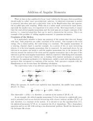
•Let {ω 1 , ω 2 ,…, ω c } be the set of c states of 

nature (“categories”) 

•Let {α 1 , α 2 ,…, α a } be the set of possible actions 

•Let λ(α i | ω j ) be the loss incurred for taking 

action α i when the state of nature is ω j

14 



Introduction 

•Overall risk R = Sum of all R(α i | x) for i = 1,…,a 

•Minimizing R(α i | x) for i = 1,…, a 

j=c 

( ) ∑ ( ) ( ) 

i i j j 

R α x = λαωP ω x 

j=1 

for i =1, L,a

15 



Introduction 

•Select the action α i for which R(α i | x) is 

minimum 

R is minimum and R in this case is called 

the Bayes risk = best performance that 

can be achieved.

16 



•Two-category classification 

• α 1 : deciding ω 1 

• α 2 : deciding ω 2 

Introduction 

• λ ij = λ(α i | ω j ) 

loss incurred for deciding ω i when the true state of 

nature is ω j 

•Conditional risk: 

•R(α 1 | x) = λ 11 P(ω 1 | x) + λ 12 P(ω 2 | x) 

•R(α 2 | x) = λ 21 P(ω 1 | x) + λ 22 P(ω 2 | x)

17 



Our rule is the following: 

if R(α 1 | x) < R(α 2 | x) 

action α 1 : “decide ω 1 ” is taken 

Introduction 

This results in the equivalent rule : 

decide ω 1 if: 

(λ 21 - λ 11 ) P(x | ω 1 ) P(ω 1 ) > (λ 12 - λ 22 ) P(x | ω 2 ) P(ω 2 ) 

and decide ω 2 otherwise

18 



•Likelihood ratio: 

Introduction 

The preceding rule is equivalent to the 

following rule: 

( ) 

( ) 

( ) 

( ) 

Pxω λ -λ P ω 

if > × 

Pxω 

λ -λ P ω 

1 12 22 

2 

2 

21 11 1 

•Then take action α 1 (decide ω 1 ) 

•Otherwise take action α 2 (decide ω 2 )

19 



•Optimal decision property 

Introduction 

• “If the likelihood ratio exceeds a threshold 

value independent of the input pattern x, we 

can take optimal actions”

20 


Introduction 

Minimum-Error-Rate Classification 

•Actions are decisions on classes 

•If action α i is taken and the true state of nature 

is ω j then: 

• the decision is correct if i = j and in error if i ≠ j 

•Seek a decision rule that minimizes the 

probability of error which is the error rate

21 


Introduction 


Introduction of the zero-one loss function: 

⎧0 

i= j 

λ( α i,ω j) 

= ⎨ i,j=1, L ,c 

⎩ 1 i ≠ j 

•Therefore, the conditional risk is: 

j=c 

( ) ( ) ( ) 

i i j j 

∑ 

R α x = λαω P ω x 

j=1 

∑ 

ji ≠ 

( ) ( ) 

j i 

= P ω x =1-P ω x 

•“The risk corresponding to this loss function 

is the average probability error”

22 


Introduction 


• Minimizing the risk requires maximizing 

P(ω i | x) (since R(α i | x) = 1 – P(ω i | x)) 

• For Minimum error rate 

Decide ω i if P (ω i | x) > P(ω j | x) ∀j ≠ i

23 


Introduction 


•Investigate the loss function: 

( 2) 

( ) 

( 1) 

( ) 

λ12 -λ P ω 

Pxω 

22 

Let θ = × = then decide ω if: >θ 

λ -λ P ω Pxω 

λ 1 λ 

21 11 1 2 

If λ is the zero-one loss function which means: 

λ = 

⎛ 0 

⎜ 

⎝ 1 

1 ⎞ 

⎟ 

0 ⎠ 

then θ = 

P 

P 

ω 

ω 

= θ 

( 2 ) 

( ) 

λ a 

1 

( 2 ) 

( ) 

⎛ 0 2 ⎞ 

2P ω 

if λ = ⎜ ⎟ then θ = = θ 

⎝ 1 0 ⎠ 

P ω 

1 

λ b

24 


Introduction 

Decision Regions: Effect of Loss Functions

25 


Introduction 

Classifiers, Discriminant 

Functions and Decision Surfaces 

THE MULTICATEGORY CASE 

Set of discriminant functions 

g i(x), i = 1,…, c 

The classifier assigns a feature 

vector x to class ω i 

if: g i(x) > g j(x) ∀j ≠ i

26 


Introduction 



•Let g i(x) = - R(α i | x) 

(max. discriminant corresponds to min. risk) 

•For the minimum error rate, we take 

g i(x) = P(ω i | x) 

(max. discrimination corresponds to max. posterior) 

In this case, we can also write: 

g i(x) = P(x | ω i) P(ω i) or 

g i(x) = ln P(x | ω i) + ln P(ω i) (ln: natural logarithm)

27 


Introduction 

General Statistical Classifier

28 


Introduction 



• Feature space divided into c decision regions 

if g i (x) > g j (x) ∀j ≠ i then x is in R i 

R i means assign x to ω i 

• The two-category case: 

• A classifier is a dichotomizer with two 

discriminant functions g 1 and g 2 

• Let g(x) ≡ g 1 (x) – g 2 (x) 

• Decide ω 1 if g(x) > 0; 

• Otherwise decide ω 2

29 


Introduction 



•The computation of g(x) 

( ) ( ) 

g(x) = P ω x -P ω x 

1 2 

( ) 

( ) 

P x ω P ω 

=ln +ln 

P x ω 

P ω 

( ) 

1 1 

2 

( ) 

2

30 


Introduction 


Functions and Decision Surfaces

31 


The Normal Density 

Introduction 

Univariate density 

-Density which is analytically tractable 

-Continuous density 

-A lot of processes are asymptotically Gaussian 

-Handwritten characters, speech sounds are 

examples or prototypes corrupted by 

random process (central limit theorem) 

1 

p ( x ) = 

e 

σ 2 π 

Where: µ = mean or expected value of x 

σ 2 = the variance of x 

− 

1 

2 

⎛ 

⎜ 

⎝ 

x − µ ⎞ 

⎟ 

σ 

⎠ 

2

32 



Introduction

33 



Introduction 

•Multivariate density 

•Multivariate normal density in d dimensions is: 

1 ⎡ 1 t -1 ⎤ 

P(x) = exp 

⎢ 

- d/2 1/2 ( x -µ ) Σ ( x-µ ) 

⎣ 

⎥ 

2π Σ 

2 

⎦ 

( ) 

where: x = (x 1 , x 2 , …, x d ) t 

µ = (µ 1 , µ 2 , …, µ d ) t mean vector 

Σ = d*d covariance matrix 

|Σ| and Σ -1 are the determinant 

and inverse, 

respectively

34 


Introduction 

Discriminant Functions for the Normal 

Density 

•We saw that the minimum error-rate 

classification can be achieved by the 

discriminant function 

g i (x) = ln P(x | ω i ) + ln P(ω i ) 

•Case of multivariate normal distribution 

1 d 1 

g(x)=- x-µ x-µ - ln2π- In Σ +InP ω 

2 2 2 

∑ -1 

i i i 

i i i 

( ) ( ) ( ) 

t

35 


Introduction 

Discrimination and Classification for 

Different Cases 

∑ 2 

i 

Case = σ I 

g (x) = w x + w (linear discriminant function) 

i 

t 

i i0 

where : 

(w is called the threshold for the ith 

i0 

category!) 

µ i 1 t 

w= i ;w 2 i0 =- µµ+lnP(ω 2 i i i) 

σ 2σ

36 


Introduction 



–A classifier that uses linear discriminant 

functions is called “a linear machine” 

–The decision surfaces for a linear machine are 

pieces of hyperplanes defined by: g i (x) = g j (x)

37 


Equal Covariances 

Introduction

38 


Introduction 



•The hyperplane separating R i and R j 

( ) 

2 

1 σ P ω 

x = ( µ +µ ) - ln µ -µ 

2 µ-µ P ω 

i ( ) 

( ) j 

0 i j 2 

i j 

i j 

• Always orthogonal to the line linking the means 

1 

if P ω =P ω then x = µ +µ 

2 

( ) ( ) ( ) 

i j 0 i j

39 


Shift in Priors 

Introduction

40 


Shift in Priors 

Introduction

41 


Introduction 



Case Σ i = Σ (covariance of all classes are 

identical but arbitrary) 

Hyperplane separating R i and R j 

ln ⎡ ( ) ( ) ⎤ 

⎣ 

P ωi P ωj 

⎦ 

( i 

t 

j) -1 ( i j) 

1 

x = ( µ +µ ) - × µ -µ 

2 µ-µ Σ µ-µ 

( ) 

0 i j i j 

(the hyperplane separating R i and R j is 

generally not orthogonal to the line 

between the means)

42 


Decision Surfaces 

Introduction

43 


Decision Surfaces 

Introduction

44 


Introduction 



Case Σ i = arbitrary 

– The covariance matrices are different for each category 

where : 

( ) 

g x = x Wx + wx+ 

w 

t 

t 

i i i i0 

1 

W=- 

2 

∑ 

∑ 

i i 

-1 

w = µ 

-1 

i i i 

1 t -1 1 

w i0 = - µ i ∑ µ i - ln ∑ + lnP( ωi 

) 

i i 

2 2 

(Hyperquadratics which are: hyperplanes, pairs of hyperplanes, 

hyperspheres, hyperellipsoids, hyperparaboloids, etc.)

45 


Decision Boundaries 

Introduction

46 



Introduction

47 



Introduction

48 


Introduction 

Bayesian Decision Theory – Discrete 

Features 

Components of x are binary or integer valued, x 

can take only one of m discrete values 

v 1 , v 2 , …, v m 

Case of independent binary features in 2 category 

problem 

Let x = (x 1 , x 2 , …, x d ) t where each x i is either 0 or 1, 

with probabilities: 

p i = P(x i = 1 | ω 1 ) 

q i = P(x i = 1 | ω 2 )

49 


Introduction 

Bayesian Decision Theory – Discrete 

Features 

The discriminant function in this case is: 

d 

∑ 

g(x) = w x + w 

where 

and 

i=1 

i i 0 

( ) 

( ) 

p i 1- q i 

w i = ln i = 1, L ,d 

q 1-p 

i i 

1-p 

( 1 ) 

( ) 

P ω 

d 

i 

w 0 = ∑ ln + ln 

i=1 1-qi P ω 2 

decide ω if g(x) > 0 and ω if g (x) ≤ 0 

1 2

Chapter 2

Create successful ePaper yourself

Delete template?

Save as template?