JavaPsi - Simulating and Visualizing Quantum Mechanics (english)

3 SOLVING SCHRÖDINGER’S EQUATION 10
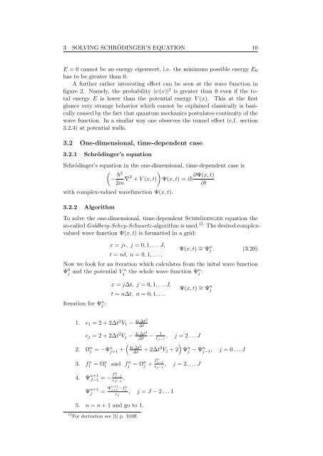
E = 0 cannot be an energy eigenwert, i.e. the minimum possible energy E0
has to be greater than 0.
A further rather interesting effect can be seen at the wave function in
figure 2. Namely, the probability |ψ(x)| 2 is greater than 0 even if the total
energy E is lower than the potential energy V (x). This at the first
glance very strange behavior which cannot be explained classically is basically
caused by the fact that quantum mechanics postulates continuity of the
wave function. In a similar way one observes the tunnel effect (c.f. section
3.2.4) at potential walls.
3.2 One-dimensional, time-dependent case
3.2.1 Schrödinger’s equation
Schrödinger’s equation in the one-dimensional, time-dependent case is
− 2
2m ∇2
∂Ψ(x, t)
+ V (x, t) Ψ(x, t) = i
∂t
with complex-valued wavefunction Ψ(x, t).
3.2.2 Algorithm
To solve the one-dimensional, time-dependent Schrödinger equation the
so-called Goldberg-Schey-Schwartz-algorithm is used. 15 The desired complexvalued
wave function Ψ(x, t) is formatted in a grid:
x = jɛ, j = 0, 1, . . . J,
t = nδ, n = 0, 1, . . . ,
Ψ(x, t) ∼ = Ψ n j . (3.20)
Now we look for an iteration which calculates from the inital wave function
Ψ 0 j
and the potential V n
j the whole wave function Ψn j :
Iteration for Ψ n j :
1. e1 = 2 + 2∆t 2 V1 −
ej = 2 + 2∆t 2 Vj −
2. Ω n j = −Ψn j+1 +
x = j∆t, j = 0, 1, . . . J,
t = n∆t, n = 0, 1, . . .
4i ∆t2
∆t
4i ∆t2
∆t
Ψ(x, t) ∼ = Ψ n j
1 − , j = 2 . . . J
ej−1
4i ∆t 2
∆t + 2∆t2 Vj + 2
3. f n 1 = Ωn1 and f n j = Ωnj + f n j−1
, j = 2, . . . J
ej−1
4. Ψ n+1
J−1 = − f n J−1
eJ−1 ,
Ψ n+1
j
Ψn+1
j+1
= −f n j
, j = J − 2 . . . 1
ej
5. n = n + 1 and go to 1.
15 For derivation see [5] p. 103ff.
Ψn j − Ψnj−1 , j = 0 . . . J