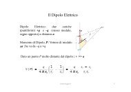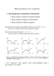
Untitled - Cdm.unimo.it

190 Polynomial Approximation of Differential Equations
Classical formulations are illustrated for instance in lions and magenes(1972). Alter-
native formulations, specifically addressed to applications in the field of spectral meth-
ods, are introduced in canuto and quarteroni(1981), maday and quarteroni(1981),
canuto and quarteroni(1982b). Following these papers, we present several useful
results. Let us begin by examining the Dirichlet problem (9.1.4). Without loss of
generality, we can assume that σ1 = σ2 = 0 (homogeneous boundary conditions). Ac-
tually, solutions corresponding to non-homogeneous boundary conditions are obtained
by adding to U the function r(x) := 1
2 (1 − x)σ1 + 1
2 (1 + x)σ2, x ∈ Ī.
Let X be a suitable functional space, for now the space C ∞ 0 (I) (see section 5.4).
Recall that φ ∈ X satisfies φ(±1) = 0. Thus, one obtains the identity
(9.3.1)
U ′ (φw) ′
dx = fφw dx, ∀φ ∈ X.
I
I
The above relation is obtained by multiplying both sides of equation (9.1.4) by φw and
integrating in I. The final form follows after integration by parts using the condition
φ(±1) = 0. In this context, φ is called a test function. It is an easy exercise to check
that, due to the freedom to choose the test functions, we start from (9.3.1) and deduce
the original equation (9.1.4). Thus, one concludes that, when U is solution to (9.3.1)
with U(±1) = 0, then it is also solution to (9.1.4) with σ1 = σ2 = 0.
The advantage of replacing (9.1.4) with (9.3.1) is that the new formulation can be
suitably generalized by weakening the hypotheses on the data and the solution. To this
end, we note that, according to (9.3.1), U is not required to have a second derivative.
This regularity assumption is substituted by appropriate integrability conditions on
U ′ and φ ′ . In order to proceed with our investigation, we need to use the functional
spaces introduced in section 5.7. Henceforth, w will be the Jacobi weight function in
the ultraspherical case, where ν := α = β satisfies −1 < ν < 1. We shall seek the
solution U in the space H 1 0,w(I) (see (5.7.6)), which is also a natural choice for the
space of test functions. Therefore, we set X ≡ H 1 0,w(I). Finally, we take f ∈ L 2 w(I)
(see (5.2.1)). As we will see, these assumptions are sufficient to guarantee the existence
of the integrals in (9.3.1), which are now considered in the Lebesgue sense.
The next step is to insure that, in spite of such generalizations, problem (9.3.1) is still