I. FOURIER SERIES, FOURIER TRANSFORM.

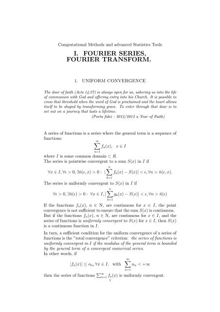
Computational Methods and advanced Statistics Tools
I. FOURIER SERIES,
FOURIER TRANSFORM.
1. UNIFORM CONVERGENCE
The door of faith (Acts 14:27) is always open for us, ushering us into the life
of communion with God and offering entry into his Church. It is possible to
cross that threshold when the word of God is proclaimed and the heart allows
itself to be shaped by transforming grace. To enter through that door is to
set out on a journey that lasts a lifetime.
(Porta fidei - 2012/2013 a Year of Faith)
A series of functions is a series where the general term is a sequence of
functions:
∞
fn(x), x 2 I
n=1
where I is some common domain ½ R.
The series is pointwise convergent to a sum S(x) in I if
n
8x 2 I, 8ǫ > 0, 9¯n(ǫ, x) > 0 : j fk(x) ¡ S(x)j < ǫ, 8n > ¯n(ǫ, x).
The series is uniformly convergent to S(x) in I if
n
8ǫ > 0, 9¯n(ǫ) > 0 : 8x 2 I, j gk(x) ¡ S(x)j < ǫ, 8n > ¯n(ǫ)
k=1
k=1
If the functions fn(x), n 2 N, are continuous for x 2 I, the point
convergence is not sufficient to ensure that the sum S(x) is continuous.
But if the functions fn(x), n 2 N, are continuous for x 2 I, and the
series of functions is uniformly convergent to S(x) for x 2 I, then S(x)
is a continuous function in I.
In turn, a sufficient condition for the uniform convergence of a series of
functions is the ”total convergence” criterion: the series of functions is
uniformly convergent in I if the modulus of the general term is bounded
by the general term of a convergent numerical series.
In other words, if
∞
jfn(x)j · αn, 8x 2 I, with αn < +1
then the series of functions ∞
n=1 fn(x) is uniformly convergent.
1
n=1

2
When such a condition is satisfied one can prove that:
i) the sum of the series of function S(x) is continuous in I;
ii) the definite integral on [a, b] ½ I of the sum of the series is equal to
the sum of the integrals of fn(x);
iii) if, moreover, the general term fn(x) is differentiable and, in the
interval I, jf ′ n (x)j is bounded by the general term of convergent numer-
ical series, the sum S(x) of the series of functions is differentiable and
the sum of the derivatives converges to S ′ (x).
For example, since
n
1
j sin(nx)j ·
n3 n
1
< +1 and
n3 n
1
jn cos(nx)j ·
n3 n
1
< +1
n2 the sum S(x) of
n sin(nx)/n3 exists, it is continuous, it admits a continuous
derivative S ′ (x), which is the sum of the series of the derivatives
8x 2 R. In such a case we say that the series can be derived term by
term. Besides, for any finite a, b with a < b,
b b
fn(x)dx = fn(x)dx
n
a
for fn(x) = sin(nx)/n 3 , as well as for fn(x) = cos(nx)/n 2 . In such
cases we say that the series can be integrated term by term.
2. FOURIER SERIES
And that [the unheard-of precision of the processes associated with the ”Big-
Bang”] is supposed to have happened by chance?! What an absurd idea!
(Walter Thirring, b.1927, physicist)
A function f is said to be periodic if it is defined for all real x and if
there is a positive number T such that
(1)
f(x + T ) = f(x), 8x
According to this definition, a constant function is periodic with arbitrary
period. Trigonometric functions, such as sin x, sin 2x, ..., sin nx,
or cos x, ..., cos nx, are periodic with period 2π. If T is a period for f
then f(x + nT ) = f(x), 8n 2 N, so that f is periodic with periods
2T, 3T, ..., too. A trigonometric polynomial is a finite sum of the form
(2)
a◦
2 +
k
(an cos nx + bn sin nx)
n=1
Any trigonometric polynomial is periodic with period 2π.
a
n

Let us assume that f(x) is a periodic function with period 2π that can
be represented by a trigonometric series,
f(x) = a◦
2 +
∞
(3)
(an cos nx + bn sin nx)
−π
−π
n=1
that is, we assume that this series converges and has f(x) as its sum.
Given such a function f(x), we want to determine the cifoefficients an
and bn of the corresponding series (3). We first determine a◦. Integrating
on both sides of (3) from ¡π to π, and assuming that term-by
term integration of the series is allowed, we have
π
f(x) dx = a◦
π ∞
π
π
dx+ an cos nx dx + bn sin nx dx .
2
n=1
The first term on the right equals πa◦. All the other integrals on the
right are zero, as can be readily seen by performing the integrations.
Hence our first result is
(4)
a◦
2
−π
π
1
= f(x) dx.
2π −π
We now determine a1, a2, ... by a similar procedure. We multiply (3) by
cos mx, where m is any fixed positive integer, and integrate from ¡π
to π term by term, we see that π
f(x) cos mx dx becomes:
−π
π
a◦
cos mx dx+
2
(5)
+
∞
·
n=1
an
−π
π
π
cos nx cos mx dx + bn
−π
−π
−π
sin nx cos mx dx .
The first integral is zero. Now by the trigonometric identities
cos α cos β = 1
[cos(α + β) + cos(α ¡ β)]
2
sin α cos β = 1
[sin(α + β) + sin(α ¡ β)]
2
we obtain
π
cos nx cos mx dx =
−π
1
π
cos(n + m)x dx +
2 −π
1
π
cos(n ¡ m)x dx,
2 −π
π
sin nx cos mx dx =
−π
1
π
sin(n + m)x dx +
2 −π
1
π
sin(n ¡ m)x dx.
2 −π
Integration shows that the four terms on the right are zero, except for
the last term in the first line, which equals π when n = m. Since in (5)
this term is multiplied by am, the whole of (5) is equal to amπ, and our
second result is
am = 1
π
(6)
f(x) cos mx dx, m = 1, 2, ...
π
−π
3

4
We finally determine b1, b2, ... in (3). If we multiply (3) by sin mx,
where m 2 N, and then integrate from ¡π to π, we have
π
π
a◦
f(x) sin mx dx =
2 +
∞
(7)
(an cos nx + bn sin nx) sin mx dx
−π
−π
1
Integrating term by term, we see that the right hand side becomes
π
∞
· π
a◦
sin mx dx+ an
2
π
cos nx sin mx dx + bn sin nx sin mx dx
−π
1
−π
The first integral is zero. The next integral is of the type considered
before, and we know that it is zero for all n 2 N. For the last integral
we need the identity
we obtain
π
sin nx sin mx dx = 1
π
2
−π
−π
sin α sin β = ¡ 1
[cos(α + β) ¡ cos(α ¡ β)]
2
−π
cos(n ¡ m)x dx ¡ 1
π
cos(n + m)x dx,
2 −π
The last term is zero. The first term on the right is zero when n 6= m
and is π when n = m. Since in (7) this term is multiplied by bm, the
right hand side in (7) is equal to bmπ, and our last result is
(8)
bm = 1
π
π
f(x) sin mx dx, m 2 N.
−π
The above calculation can be performed for a periodic function with
any period T > 0, (f(x) = f(x + T ), 8x 2 R). Besides, since the
integrals (4,6, 8) exist under wide conditions (e.g. if f is piecewise
continuous), we give the following definition:
DEF. 2.A (Fourier series) If f(x) is a piecewse continuous, periodic
function with period 2π, the Fourier series associated with f(x) is the
(formal) series
(9)
f(x) » a◦
2 +
∞
(an cos nx + bn sin nx)
n=1
where the Fourier coefficients an, bn are given by:
an = 1
π
(10)
f(x) cos nx dx, n = 0, 1, 2, ...
π
(11)
−π
bn = 1
π
f(x) sin nx dx, n = 1, 2, ...
π −π

More generally, for a piecewise continuous, periodic function with period
T , the associated Fourier series is
f(x) » a◦
2 +
∞
·
an cos( 2π
T nx) + bn sin( 2π
T nx)
(12)
n=1
with Fourier coefficients:
an = 2
(13)
T
T/2
(14)
4
bn = 2
T
−T/2
T/2
−T/2
f(x) cos( 2π
nx) dx, n 2 N◦
T
f(x) sin( 2π
nx) dx, n 2 N
T
REMARK 2.B - a) An equivalent choice is to express the coefficients
by integrals from 0 to T , by virtue of periodicity of the function f:
an = 2
T
f(x) cos(
T 0
2π
(15)
nx) dx, n 2 N◦
T
bn = 2
T
f(x) sin(
T 0
2π
nx) dx, n 2 N
T (16)
Actually the same numbers are obtained by integrating on any interval
[c, c + T ], with fixed c 2 R.
b) The symbol » reminds that the trigonometric expansion is still
formal: by that symbol nothing is said about convergence, and, if the
series is convergent, the sum is not necessarily f(x).
c) The constant term in (12), i.e. a◦/2 = 1
T
f(x) dx, is the mean
T 0
value of f in one period.
REMARK 2.C - Coefficients of the Fourier series in exponential form.
- If the Fourier series of a T ¡ periodic function f(x) is in exponential
form, i.e.
then the coefficients are
f(x) »
cn = 1
T
T
0
+∞
n=−∞
2π
i
cne T nx
2π
−i
f(x)e T nx dx
The exponential Fourier series is equivalent to the trigonometric Fourier
series.
Proof. Take, for simplicity, T = 2π. As above, integrating term by
term 2π
f(x)dx = 2πc◦ +
[ einx
0 = 2πc◦
0
n=0
in ]2π
5

6
so that c◦ is the mean of the periodic function.
Multiplying both sides by e−imx , m 6= 0, and integrating we find:
2π
f(x)e −imx dx = e
[cn
i(n−m)x
i(n ¡ m) ]2π 0 + 2πcm
0
n=m
so that cm = (2π) −1 2π
0 f(x)e−imx dx as stated.
Of course the equivalence depends on the Euler identity: e inx =
cos(nx) + i sin(nx). 4
3. THEOREMS ON FOURIER SERIES
[God] desires all men to be saved and come to the knowledge of the truth.
( 1 Tim 2:4 )
THEOREM 3.A (A priori bound on Fourier coefficients)
If the periodic function f admits continuous r¡th derivative in [0, T ]
with r ¸ 1, then the coefficients of the Fourier exponential series satisfy
jcnj · cjnj −r , 8n 2 Z,
where the constant c is independent of n. Similarly, janj · ˜cn −r , jbnj ·
˜cn −r , if an, bn are the coefficients of the trigonometric series.
Proof. - Let f 2 Cr ([0, T ]). The derivative of a periodic function is
still periodic, so integrating by parts r times the expression (?? )
cn = 1
·
f(x)
T
T
2π
e−i T
¡i2πn nx
T T
¡ f ′ (x) T
2π
e−i T
¡i2πn nx
dx
= + 1
T
Therefore
where
T
T
f
i2πn 0
′ 2π
−i
(x)e T nx dx = + 1
T
jcnj · 1
T
0
0
· T
i2πn
r T
·
T
r T
2πjnj 0
· 1
T jnjr · r T
T
jf
2π 0
(r) (x)j dx · c
jnjr c =
· r T
2π
jf (r) 2π
−i
(x)jje T nx j dx
max
x∈[0,T ] jf (r) (x)j.
0
f (r) 2π
−i
(x)e T nx dx.
Since an ¡ ibn = 2cn, choosing ˜c = 2c the proof is complete. 4

Def. A function f(x) is said piecewise continuous in (a, b) ½ R if f
is defined and continuous except in a finite number of points xj 2 (a, b),
j = 1, ..., N, where there exist the finite limits:
f(xj + 0) = limx→xj+(x), f(xj ¡ 0) = limx→xj−f(x).
Such type of regularity is part of the Dirichlet condition, assumed in
the most usual convergence result, that we state without proof:
THEOREM 3.B (Dirichlet’s Criterion) Let the function f(x) be periodic
(with period T ). Let both f(x) and f ′ (x) be piecewise continuous.
Then the trigonometric series associated with f is convergent to f(x)
in each point where f is continuous; while in each point x◦ where f is
discontinuous, the series is convergent to the half-sum
f(x◦ + 0) + f(x◦ ¡ 0)
.
2
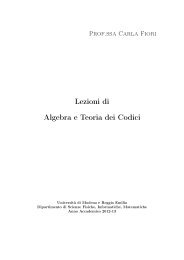
EXAMPLE 3.C (Fourier expansion of a periodic step function) - Let
1 x 2 [2nπ, (2n + 1)π]
f(x) =
0 elsewhere.
which satisfies the Dirichlet conditions, with period T = 2π. The
Fourier coefficients a◦, an, bn are directly calculated:
π
a◦ 1
= f(x) dx =
2 2π
1
π
1 dx =
2π
1
2 .
−π
For n 2 N,
an = 1
π
f(x) cos(nx) dx =
π −π
1
π
cos(nx) dx =
π 0
1
· π sin(nx)
= 0,
π n 0
bn = 1
π
f(x) sin(nx) dx =
π −π
1
π
sin(nx) dx =
π 0
1
·
¡
π
cos(nx)
π =
n 0
= 1
nπ [1 ¡ (¡1)n
0, n even
] = 2 , n odd .
nπ
Thus bn vanishes for even n, it equals 2
nπ
is:
1
2 +
∞
[an cos(nx) + bn sin(nx)] = 1
2 +
n=1
0
for odd n. The Fourier series
∞
n=0
2
sin [(2n + 1)x] .
(2n + 1)π
REMARK 3.D - (On the computation of Fourier coefficients)
7

8
0.0 0.2 0.4 0.6 0.8 1.0
−5 0 5
Figure 1. Graph of the Fourier series calculated by the
first 25 harmonics, i.e. for n from 0 to 12.
a) In order to compute the coefficients of the Fourier series, several
remarks are useful.
A function f(x) is said to be even if f(¡x) = f(x), 8x; it is odd if
f(¡x) = ¡f(x), 8x. If the function f(x) is even, then all the Fourier
coefficients bn vanish: indeed, under a substitution y = ¡x,
bn = 2
T
T 0
T/2
2
f(¡y) sin(¡
T
2π
2
ny) dy = ¡
T T
−T/2
f(x) sin( 2π 2
nx) dx =
T T
x
T/2
−T/2
T/2
−T/2
f(x) sin( 2π
nx) dx =
T
f(y) sin( 2π
ny) dy = ¡bn
T
Thus 2bn = 0, so that bn = 0. Similarly, it turns out that a◦ = an = 0
if the function is odd.
b) Therefore an even periodic function admits a series expansion with
only cosine terms; while an odd periodic function admits a series
expansion with only sine terms. The next remark regards an arbitrary
function f(x), defined in some interval, for example in (0, π). We can
extend it both to an even function and to an odd function. Indeed,
we can define it in the interval (¡π, 0) so that it becomes even:
⎧
⎤
⎨ f(x), x 2 (0, π)
f◦(x) = limx→0+ f(x), x = 0 ⎦
⎩
f(¡x), x 2 (¡π, 0)
Another choice is to define an odd extension of f(x):
⎧
⎤
⎨ f(x), x 2 (0, π)
f1(x) = 0, x = 0 ⎦
⎩
¡f(¡x), x 2 (¡π, 0)

Finally, one can extend the functions f◦(x) and f1(x) to the whole of
R, so that the resulting function is periodic with period 2π. Assuming
the Dirichlet conditions to hold, it follows that
(17)
where
and
(18)
f◦(x) = 1
2 a◦ +
∞
an cos(nx)
n=1
an = 1
π
f◦(x) cos(nx) dx =
π −π
2
π
f(x) cos(nx) dx
π 0
f1(x) =
∞
bn sin(nx)
n=1
where
bn = 1
π
f1(x) sin(nx) dx =
π −π
2
π
f(x) sin(nx) dx
π 0
(indeed f1(x)sin(nx) is even, as a product of two odd functions). Now
under a restriction of (17), (18) to the interval (0, π), it follows that a
function with domain (0, π) can be expanded in a cosine-series as well
as in a sine-series.
4. APPLICATION OF THE FOURIER SERIES TO
DIFFERENTIAL EQUATIONS
To believe in a God means to realize that the facts of the world are not the
whole story. To believe in a God means to realize that life has a meaning.
(Ludwig Wittgenstein, 1889-1951)
EX. 4.A - The damped harmonic oscillator with a periodic force
Let us compute a particular solution of the damped harmonic oscillator
with a forcing term
(19)
¨x + µ ˙x + ω 2 x = f(t)
when f(t) is a real valued periodic function with period T . Although
not real-valued, it is convenient first to consider
where Ω = 2π
T
f(t) = ρ ¢ e iΩt
is the pulsation of the forcing term. In this case a
particular solution in the form const. ¢ eiΩt is easily found:
x ∗ (t) =
ρe iΩt
ω 2 ¡ Ω 2 + iΩµ
9

10
As a second step let us consider f(t) given by a finite Fourier expansion
in exponential form:
N
f(t) = cne iΩnt
n=−N
where cn = ¯c−n since f(t) is real valued. A particular solution with
period T is given by
x ∗ (t) =
N
x ∗ n(t), x ∗ n(t) =
n=−N
cne iΩnt
ω 2 ¡ n 2 Ω 2 + inΩµ
Notice that x∗ is real since the addends of the sum with opposite indices
n, ¡n are complex conjugate. Moreover x∗ n (t) is a particular solution
of the differential equation
¨x + µ ˙x + ω 2 x = cne iΩnt .
Thus we can immediately verify:
¨x ∗ + µ ˙x ∗ + ω 2 x ∗ N
= (¨x ∗ n + µ ˙x ∗ n + ω 2 x ∗ n) =
n=−N
N
n=−N
cne iΩnt = f(t).
Finally, let f(t) admit a Fourier expansion with infinitely many nonzero
coefficients:
f(t) =
∞
n=−∞
cne iΩnt
A particular solution is looked for in the form:
x ∗ (t) =
∞ cn
ω2 ¡ n2Ω2 + inΩµ eiΩnt
(20)
n=−∞
To this end we have to check the convergence of (20); then, provided
its convergence, to check whether is it a solution of the differential
equation. Now a sufficient condition to derive k times term by term
is the convergence of the series of the k¡th order derivatives:
(21)
∞
n=−∞
cn(iΩn) k
ω 2 ¡ n 2 Ω 2 + inΩµ eiΩnt
uniformly with respect to t. On the other hand we know that f 2 C r
implies the bound on the Fourier coefficients jcnj · cn −r . Therefore
the general term of (23) is bounded by
cΩ k
n k
nr (ω2 ¡ n2Ω2 ) 2 + n2 µ 2 · Cnk−r−2
Ω2 for some constant C > 0 independent of n. So the series (23) is uniformly
convergent with respect to t if
r + 2 ¡ k > 1;

In particular, the series (20) is a solution of the differential equation if
r + 2 ¡ 2 > 1 (k = 2), i.e. if the function f(t) is at least in C 2 .
Notice: for µ small enough, the particular solution x ∗ (t) amplifies the
harmonics n = §[ω/Ω], (where [¢] denotes the integral part), of the
function f(t) for which ω 2 ¡n 2 Ω 2 attains its minimum, while the other
harmonics are damped.
EXAMPLE 4.B Let us consider the one-dimensional heat equation
with boundary and initial conditions:
⎧
∂u ⎨ ∂t
⎩
= 2 ∂2u ∂x2 (22) u(0, t) = u(3, t) = 0,
u(x, 0) = 5 sin(4πx) ¡ 3 sin(8πx) + 2 sin(10πx),
⎤
8t ¸ 0 ⎦
x 2 [0, 3].
Besides, the solution is required to remain bounded 8(x, t) 2 [0, 3]£R + .
Let us solve the equation by separation of variables. By such a method,
we look for a solution (if possible) of the form
u(x, t) = f(x)g(t)
. Then the equation reads f(x) ˙g(t) = 2f ′′ (x)g(t). After separating
variables,
2 ¢ f ′′ (x) ˙g(t)
=
f(x) g(t) .
Since the left hand side depends only on x, the right hand side depends
only on t, and the equation holds for all (x, t) where x, t are independent
variables,
9λ 2 R : 2 f ′′ (x) ˙g(t)
= 2λ =
f(x) g(t) .
Therefore we obtain two ordinary differential equations depending on
an arbitrary parameter λ:
with general solutions
(23)
f ′′ = λf, ˙g = 2λg
f(x) = c1e √ λx + c2e −√ λx , g(t) = ce 2λt
if λ 6= 0
f(x) = c1x + c2, g(t) = c if λ = 0.
Now, the boundedness requirement 8t 2 R + implies λ < 0. Therefore,
setting λ = ¡ω2 and c1 = 1
2 (a + ib = ¯c2, the general solutions (23) can
be written:
f(x) = a cos(ωx) + b sin(ωx), g(t) = ce −2ω2 t .
Hence a solution of the heat equation turns out to be
u(x, t) = f(x)g(t) = ce −2ω2 t [a cos(ωx) + b sin(ωx)] =
= e −2ω2 t [A cos(ωx) + B sin(ωx)]
11

12
u(x,t)
−5 0 5
0.0 0.5 1.0 1.5 2.0 2.5 3.0
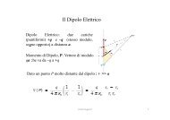
Figure 2. Graph of the function u(x, t) for some values of
t: t = 0 (continuous line), t = 0.001 and t = 0.01
with constants A, B, ω to be determined by using the boundary conditions
in (??):
u(0, t) = 0 =) A = 0, i.e. u(x, t) = e −2ω2 t B sin(ωx)
u(3, t) = 0 =) B sin(3ω) = 0
This last equality, in turn, implies
either B = 0, arbitrary ω, or arbitrary B, ω = nπ/3, n 2 Z.
Now B = 0 is immediately rejected since it gives an identically vanishing
solution. Therefore a nontrivial solution of the diffusion equation
in (??) with zero boundary condition has the form:
u(x, t) = Be −2n2π2t/9 nπ
sin( x), n 2 N
3 (24)
By the superposition principle (which holds for linear differential equations),
the sum of solutions of a homogeneous differential equation is
still a solution; so for any choice of n1, n2, n3 2 N the function
B1e −2n2 1π2t/9 n1π
sin(
3 x)+B2e −2n2 2π2t/9 n2π
sin(
3 x)+B3e −2n2 3π2t/9 n3π
sin(
3 x)
is still a solution of the equation in (??). By comparing this type of
solution with the initial condition in (??) we find:
B1 = 5, n1π/3 = 4π, B2 = ¡3, n2π/3 = 8π, B3 = 2, n3π/3 = 10π
i.e. n1 = 12, n2 = 24, n3 = 30. Thus the unique (bounded) solution
of the diffusion problem (??) is
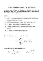
u(x, t) = 5e −32π2 t sin(4πx) ¡ 3e −128π 2 t sin(8πx) + 2e −200π 2 t sin(10πx)
x

u(x,t)
5
0
−5
0.0
0.5
1.0
1.5
x
2.0
2.5
3.0
0.000
0.002
0.006
t
0.004
0.010
0.008
Figure 3. Graph of the function u(x, t), for (x, t) 2 (0, 3) £ (0, 0.01)
EXAMPLE 4.C - We solve the same diffusion equation with a different
initial value function:
⎧
⎨
⎩
∂u
∂t = 2 ∂2u ∂x2 u(0, t) = u(3, t) = 0, 8t ¸ 0
u(x, 0) = 25x(3 ¡ x), x 2 [0, 3]
Again by separation of variables we obtain a solution of the heat equation,
but it is no more sufficient to make a finite superposition of such
functions to solve the problem. We try by a superposition of infinitely
many functions:
u(x, t) =
∞
n=1
Bne −2n2 π 2 t/9 sin(n π
3 x),
where we require u(x, 0) = 25x(3 ¡ x), that is
25x(3 ¡ x) =
∞
n=1
⎤
⎦
Bn sin(n π
x), x 2 (0, 3).
3
This amounts to expand in a sine Fourier series the function 25x(3¡x).
According to Remarks 2 (b), this is possible if we regard the function
as a restriction of an odd periodic function defined for all x 2 R, with
period 6:
⎧
⎤
⎨ 25x(3 ¡ x), x 2 (0, 3)
f2(x) = 25x(3 + x), x 2 (¡3, 0) ⎦
⎩
... and so on.
13

14
u(x,t)
0 10 20 30 40 50
0.0 0.5 1.0 1.5 2.0 2.5 3.0
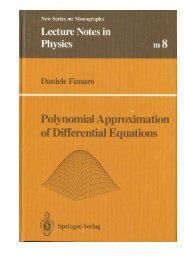
Figure 4. For initial shape u(x, 0) = 25x(3 ¡ x), graph of
the solution u(x, t) when t = 0, t = 0.01, t = 0.1
Then we have the usual Fourier coefficients for an odd function of
period T :
Bn = 2
T/2
f2(x) sin(n
T −T/2
2π
T/2
4
x) dx = f2(x) sin(n
T T 0
2π
x) dx =
T
= 2
3
25x(3 ¡ x) sin(nπx/3) dx =
3 0
900
n3π3 [1 ¡ (¡1)n ]
Finally
u(x, t) 1800
π3 ∞
(2m + 1) −3 e −2(2m+1)2π2 t/9
sin((2m + 1)πx/3).
m=0
The graph of u(x, t) is first represented for some values of t (Fig. 4),
then for (x, t) 2 (0, 3) £ (0, 1) (Fig. 5).
5. FOURIER TRANSFORM
Mans’s unique grandeur is ultimately based on his capacity to know the truth.
And human beings desire to know the truth.
Yet truth can only be attained in freedom. This is the case for all truth,
as is clear from the history of science; but it is eminently the case with
those truths in which man himself, man as such, is at stake, the truths of
the spirit, the truths about good and evil, about the great goals and horizons
of life, about our relationship with God. These truths cannot be attained
without profound consequences for the way we live our lives.
(Benedict XVI)
x

u(x,t)
t
Figure 5. For initial shape u(x, 0) = 25x(3 ¡ x), graph of
the solution u(x, t), (x, t) 2 (0, 3) £ (0, 1)
DEFINITION 5.A (Direct Fourier transform) Let the function f(t) be
given for any t 2 R. If the integral
∞
0
f(t)e −iωt dt
exists 8ω 2 R, then f(t) is said to admit the Fourier transform ˆ f(ω) :
F (f) = ˆ +∞
f(ω) = f(t)e −iωt (25)
dt.
−∞
The operator F , which transforms f(t) into ˆ f(ω), is said ”Fourier
transform”.
Usually the variable t is a time variable, in which case the variable ω is
a frequency. The Fourier transform ˆ f(ω) is a complex valued function
that can be written in exponential notation as
ˆf(ω) = A(ω)e iφ(ω)
where the real function A(ω) is said Fourier spectrum, A 2 (ω) is the
power spectrum, and φ(ω) is the phase angle.
REMARK 5.B The complex conjugate of ˆ f(ω) is equal to the Fourier
transform of the conjugate of f calculated in ¡ω:
+∞
¯ˆf(ω) = ( f(t)e −iωt dt) ¯ +∞
= ¯f(t)e iωt dt = ˆ¯ f(¡ω).
−∞
In particular, if f(t) is a real valued function, then A(ω) = A(¡ω), i.e.
A(ω) is an even function.
−∞
x
15

16
p_a(x)
0.0 0.2 0.4 0.6 0.8 1.0
indicatore di [−a,a]
−a a
Figure 6. Graph of pa(t).
EXAMPLE 5.C We want to determine the Fourier transform of the
indicator function of the interval [¡a, a],
1, t 2 [¡a, a]
(26)
pa(t) =
0, jtj > a
where a > 0 is fixed. In this case the Fourier transform (25) reduces
to the integral
a
ˆpa(ω) = e −iωt · −iωt a
e
dt =
¡iω
= eiωa ¡ e−iωa sin ωa
= 2
iω ω
−a
for ω 6= 0 (while ˆpa(0) = 2a). Fig. 6 and Fig. 7 show pa(t) and ˆpa(ω),
respectively.
EXAMPLE 5.D No sufficient condition for the existence of the Fourier
transform has yet been stated. The expression (25) easily suggests that
if the function f(t) is absolutely integrable on R, that is
(27)
∞
−∞
−a
jf(t)j dt < +1,
then ˆ f(ω) exists for any ω 2 R. In other words, under this assumption
the integral (25) exists and is finite. Such a condition is sufficient but
not necessary. Indeed there exist functions, such as sin(ω◦t)/ω, for
which the Fourier transform exists, but the property (27) does not
hold.
The following is a regularity property.

Trasf. di Fourier di p_a(t)
2a
p ^ (ω)
Figure 7. Graph of ˆpa(ω).
THEOREM 5.E - If f(t) is absolutely integrable, and let ˆ f(ω) be its
Fourier transform. Then
i) limω→±∞ ˆ f(ω) = 0 (Riemann’s lemma)
ii) ˆ f(ω) is continuous on R.
Proof. We omit the proof of the first assertion, which is known as
”Riemann’s lemma”.
As for continuity, let ω◦ 2 R be fixed, and let
∆ ˆ f = ˆ f(ω) ¡ ˆ +∞
f(ω◦) = f(t)[e −iωt ¡ e −iω◦t ] dt =
We need to prove that
−∞
+∞
= f(t)e −iω◦t [e −i(ω−ω◦)t ¡ 1] dt.
−∞
8ǫ > 0, 9δ(ǫ) > 0 : jω ¡ ω◦j < δ =) j∆ ˆ fj < ǫ.
Since f(t) is absolutely integrable, there is R = R(ǫ) > 0 such that
−R +∞
jf(t)jdt + jf(t)jdt · 1
4 ǫ.
−∞
Besides, for such R = R(ǫ) we choose δ(R(ǫ)) such that
max
t∈[−R,R] ¢je−iδt ¡ 1j · 1
2 ǫ
+∞
jf(t)jdt
Now using
and
R
−∞
je −i(ω−ω◦)t ¡ 1j · je −i(ω−ω◦)t j + 1 = 2
−1
je −i(ω−ω◦)t ¡ 1j · je −iδt ¡ 1j, for jω ¡ ω◦j · δ, δt · π/2,
17

18
it follows that
j∆ ˆ · −R +∞ R
fj · 2 jf(t)jdt + jf(t)jdt + jf(t)jje
−∞
R
−R
−i(ω−ω◦)t ¡ 1jdt
· 1 1
ǫ + ǫ = ǫ
2 2
whenever jω ¡ ω◦j · δ. 4
Now let us consider the inversion problem, assuming f(t) absolutely integrable
on R. If ˆ f(ω) = F (f), the problem is how to reconstruct f(t)
starting from ˆ f(ω). The following inversion theorem is stated without
proof.
PROPOSITION 5.F (Inverse Fourier transform) - Let the function f(t)
be absolutely integrable on R and let f(t), f ′ (t) be piecewise continuous
in any bounded interval. Then the inversion formula
(28)
f(t) = 1
2π P
+∞
−∞
ˆf(ω)e iωt dω = 1
2π lim
R→+∞
+R
−R
ˆf(ω)e iωt dω
holds in all points t where f(t) is continuous, while the formula
1
2 [f(t◦ + 0) + f(t◦ ¡ 0)] = 1
2π P
+∞
ˆf(ω)e iωt (29)
dω
holds in all discontinuity points t◦. The operator F −1 trasforming ˆ f(ω)
into f(t) (at least where f is continuous) is said the inverse Fourier
transform. 4
REMARK 5.G - The integral in (28)is computed as a Cauchy principal
value. The integral
is convergent as a Cauchy Principal Value if
+R
the limit limR→+∞ (...) exists and is finite. Recall that the usual
−R
generalized integral of a function g(t) is convergent if the double limit
R
lim g(t) dt
R,S→+∞
−S
exists and is finite with R, S diverging to +1 independently of each
other. Of course if the integral is convergent in the generalized sense,
then it is convergent in the sense of the Cauchy principal value. But
the opposite implication is not true in general. An example is the
function g(t) = t, which is integrable in the Cauchy principal value
sense:
+∞
+R
P
−∞
t dt = lim
R→+∞
−R
t dt = 0.
The same function is not integrable in the generalized sense, since many
different values are attained by the double limit prescription: for example
R
−2R tdt ! ¡1, while 2R
tdt ! +1. A similar situation regards
−R
any odd, piecewise continuous function.
−∞

REMARK 5.H In some textbooks the direct ad the inverse Fourier
transforms are defined in a slightly different way, attributing to both
the same coefficient 1/ p 2π (instead of 1 and 1/2π, respectively). Actually
any other choice is good, provided that the product of the two
coefficients is 1/2π.
REMARK 5.I - (Symmetry property) If ˆ f(ω) is the Fourier transform
of f(t) (and if both satisfy the hypotheses of Theorem 5.3) then the
Fourier transform of ˆ f(t) is 2πf(¡ω), at least in the points in which f
is continuous. Indeed
F ( ˆ +∞
f) = ˆf(t)e −iωt dt = 2π 1
+∞
ˆf(t)e
2π
−iωt dt = 2πf(¡ω).
−∞
−∞
EX. 5.L Compute the Fourier transform of
f(t) = sin(ω◦t)
.
t
By Example 5.C, the indicator function pa(t) of the interval (¡a, a),
admits Fourier transform
ˆpa(ω) = 2 sin(ωa)
.
ω
Hence the given function f(t) can be seen as a Fourier transform:
f(t) = sin(ω◦t)
=
t
1
2 ˆpω◦(t),
where pω◦ is the indicator function of (¡ω◦, ω◦). Finally, by the symmetry
property
ˆf(ω) ´ 1
2 F [ˆpω◦](ω) = 2π 1
2 pω◦(¡ω)
at least in the points where pω◦ is continuous. Explicitly the result is:
(30)
(31)
if f(t) = sin(ω◦t)
,
t
then
⎧
⎨ π,
ˆf(ω)
1
= π,
⎩ 2
0,
⎤
jωj < ω◦
ω = §ω◦ ⎦
jωj > ω◦
EX. 5.M - Compute: a) the Gauss integral +∞
−∞ e−αt2dt
; b) the
Fourier transform of the Gauss function e−αt2 (α > 0).
a) Let I = +∞
−∞ e−αx2dx.
By Fubini’s theorem
2 I 2 · +∞
=
−∞
e −αx2
dx
+∞
=
−∞
e −αx2
dx
+∞
−∞
e −αy2
dy
19

20
+∞ +∞
=
−∞
−∞
e −α(x2 +y 2 ) dxdy
Under a change of variables from cartesian to polar coordinates,
x = r cos θ
y = r sin θ
, dxdy ! rdrdθ
the integral becomes
I 2 2π +∞
=
So I = π/α.
b)
0
0
e −αr2
rdrdθ = 2π[e −αr2
/(¡2α)] +∞ π
0 =
α .
F [e −αt2
] = e
R
−iωt e −αt2
dt = e
R
−(√αt+ iω
2 √ α )2 ω2
−
¢ e 4α dt
Now by Cauchy’s theorem of complex analysis, the integral performed
on the line R + iω
2 √ (parallel to the real line in the complex plane) is
α
equal to the integral performed on the real line, which is π
α :
= e −(√αt) 2 ω2
−
¢ e 4α dt =
R
π ω2
e− 4α .
α
Therefore, up to a coefficient, the Fourier transform of a Gauss function
is still a Gauss function, with α replaced by ¡1/(4α).
6. PROPERTIES OF THE FOURIER TRANSFORM
Revelation means that God opens himself, shows himself, and speaks to the
world voluntarily.
”All that is said about God presupposes something said by God” (Edith Stein)
THEOREM 6.A (Linearity property) Let the functions f1, f2 admit
Fourier transform F (f1) = ˆ f1 and F (f2) = ˆ f2, respectively. Then for
arbitrary coefficients c1, c2 2 C there exists the Fourier transform of
c1f1(t) + c2f2(t) and
F (c1f1 + c2f2) = c1 ˆ f1 + c2 ˆ f2.
Proof. A straightforward consequence of the linearity property of the
integral. F and F −1 are linear operators, too. 4.
THEOREM 6.B (Frequency shifting) Let the function f(t) admit
Fourier transform ˆ f(ω). For any constant ω◦ 2 R,
F [e iω◦t f(t)] = ˆ f(ω ¡ ω◦).

Proof.
Trasf. di Fourier di p_a(t)cos(omega0 t)
Figure 8. Graph of the Fourier transform of the modulated
indicator function pa(t) cos(ω◦t), with ω◦ = 7, a = 5.
F [e iω◦t +∞
f] = f(t)e −i(ω−ω◦)t dt = ˆ f(ω ¡ ω◦) 4
−∞
EX. 6.C Compute the Fourier transform of the modulated indicator
function
f(t) = pa(t) cos(ω◦t),
where pa(t) is the indicator of (¡a, a) and ω◦ is real and fixed. By Euler’s
formula, linearity, frequency shifting and by the above examples,
ˆf(ω) = F [pa(t) cos(ω◦t)] = 1
2 [F (pa(t)e iω◦t
) + F (pa(t)e −iω◦t
)]
= 1
2 [ˆpa(ω ¡ ω◦) + ˆpa(ω + ω◦)]
= sin[a(ω ¡ ω◦)]
ω ¡ ω◦
+ sin[a(ω + ω◦)]
.
ω + ω◦
THEOREM 6.D (Time shifting) Let the function f(t) admit Fourier
transform ˆ f(ω). Then
Proof.
F [f(t ¡ t◦)] = e −iωt◦ ˆ f(ω).
+∞
F [f(t ¡ t◦)] = f(t ¡ t◦)e −iωt dt
−∞
= e −iωt◦
+∞
f(t ¡ t◦)e −iω(t−t◦) dt
−∞
21

22
= e −iωt◦
+∞
f(t)e −iωt dt = e −iωt◦ ˆ f(ω). 4
−∞
THM. 6.E (Time scaling) Let the function f(t) admit Fourier transform
ˆ f(ω) and let a 2 R ¡ f0g be fixed. Then
F [f(at)] = 1
jaj ˆ f( ω
a ).
Proof. If a < 0 the change of variable τ = at changes the extreme
value ¡1 into +1 and vice-versa, so that
+∞
F [f(at)] = f(at)e
−∞
−iωt +∞
dt = −∞ f(τ)e−iωτ/a dτ/a, a > 0
¡ +∞
−∞ f(τ)e−iωτ/a dτ/a, a < 0
= 1
+∞
f(τ)e
jaj
−iωτ/a dτ = 1
jaj ˆ f( ω
). 4
a
−∞
Let us prove that the Fourier operator transforms derivatives in the
time representation into multiplication by corresponding monomials in
the frequency representation, and vice-versa. This property makes the
Fourier transform able to solve differential equations.
THM. 6.F (Transformation of derivatives into multiplications and viceversa)
Let f 2 C n (R) and let f (r) (t) be absolutely integrable on R for
each r · n. Then
F [f (n) ] = (iω) n ˆ f(ω).
Similarly, assuming that t n f(t) is absolutely integrable,
F [(¡it) n f(t)] = dnf(ω) ˆ
.
dωn Proof. The proof is based on integration by parts and the fact that
(32)
lim
t→±∞ f (r) (t) = 0, r = 0, 1, ..., n ¡ 1
since f (r) (t), r = 0, 1, . . . , n is absolutely integrable on R. We can
realize this fact by writing
f (r) (t) = f (r) t
(0) + f (r+1) (τ)dτ.
Since f (r+1) (τ) is absolutely integrable, then the following limit exists
and is finite:
L = lim
t→+∞ f (r) (t) = f (r) +∞
(0) + f (r+1) (τ)dτ.
Now, either L = 0 or L 6= 0 : we prove that the second case is impossible.
Ab absurdo, let L 6= 0. Then there is an interval [T, +1) in which
0
0

jf (r) (t)j > L/2, so that f (r) (t) cannot be absolutely integrable. Thus
(32) is proved. Consider
F (f (n) +∞
)(ω) = f (n) (t)e −iωt dt
−∞
= f (n−1) (t)e −iωt+∞
+ iω
−∞
+∞
f (n−1) (t)e −iωt dt
−∞
= iω F (f (n−1) )(ω)
since limt→±∞ f (n−1) (t) = 0. By iterating such relation the statement
follows. Finally, by direct inspection the trasform of (¡it)f(t) is equal
to d ˆ f(ω)/dω, and the iteration on n concludes the proof. 4
7. CONVOLUTION PRODUCT
That is one of the reasons why I believe Christianity: it is a religion that no
one could have thought up.
(C.S.Lewis, 1898-1963)
DEFINITION 7.A -(Convolution product) The convolution product of two
functions f1(t), f2(t) defined for t 2 R, is the generalized integral (provided
it exists)
+∞
(33)
(f1 ¤ f2)(t) = f1(x)f2(t ¡ x)dx.
−∞
REMARK 7.B - For the convolution product the usual associative and distributive
(with respect to sum) properties hold. Moreover, the commutative
property can be easily proved: by a change of variable t ¡ x = y,
+∞
+∞
f1 ¤ f2(t) = f1(x)f2(t ¡ x)dx = f1(t ¡ y)f2(y)dy = f2 ¤ f1(t).
−∞
THM. 7.C - (Convolution theorem in time domain, convolution theorem in
frequency domain)
If the functions f1, f2 are sufficiently regular 1 then
(34)
(35)
Scheme of proof.
−∞
F (f1 ¤ f2)(ω) = ˆ f1(ω) ¢ ˆ f2(ω)
F −1 ( ˆ f1 ¤ ˆ f2)(t) = (f1 ¤ f2)(t).
1 A generic assumption of regularity so as to ensure the existence of the Fourier
transforms, the change in the order of integration, etc.
23

24
Let us consider the fourier transfor of a convolution product:
+∞
F (f1 ¤ f2)(ω) = e −iωt +∞
dt f1(x)f2(t ¡ x)dx
−∞
−∞
+∞ +∞
=
e −iωt f1(x)f2(t ¡ x)dt dx
−∞
−∞
By the change of variables (t, x) ! (y, x), where x = x and y = t ¡ x, we
obtain
+∞ +∞
F (f1 ¤ f2)(ω) =
e −iω(x+y) f1(x)f2(y)dy dx
−∞
and vice-versa
−∞
−∞
+∞
= e −iωx +∞
f1(x) dx e −iωy f2(y) dy = ˆ f1(ω) ¢ ˆ f2(ω)
F −1 ˆ f1 ¢ ˆ f2
−∞
(t) = (f1 ¤ f2) (t) 4
EXAMPLE 7.D - (The diffusion equation on a line) Consider the heat
equation with initial condidion f(x) for 2 R:
⎧
⎨ ∂u
∂t = k
⎩
∂2u ∂x2 ⎤
u(x, 0) = f(x), ¡1 < x < +1 ⎦
ju(x, t)j < M, ¡1 < x < +1, t > 0
In this problem it is useful to consider the Fourier transform of both sides
with respect to x, so that the second order derivative (with respect to x)
is transformed into a multiplication by the square of the conjugate variable
(Thm. 6.5). Denoting p the Fourier variable conjugate with x, we obtain:
dF [u]
dt = ¡kp2 ¢ F [u]
where the Fourier transform of u is denoted by F [u]. Here we deal with a
first order ordinary differential equation, since the unknown function F [u]
no more depends on x. The general solution of such ordinary equation is:
(36)
Setting t = 0 in (36) we see that
F [u(x, t)] = Ce −kp2 t
F [u(x, 0)] = F [f(x)] = C
so that
F [u] = ˆ f(p) ¢ e −kp2t .
Now we can apply the convolution theorem (Thm. 7.1):
u(x, t) = f(x) ¤ F −1 [e −kp2
t
]
From (??) we know that
F [e −αx2
] =
With α = 1/4kt, it implies
π
α e−p2 /4α , or F −1 [e −p 2 /(4α) ] =
F −1 [e −kp2 t ] =
1
4kπt e−x2 /4kt .
α
π e−αx2

u(x,t)
0.0 0.2 0.4 0.6 0.8 1.0
u(x,t) per t=0.01,t=1,t=10
t=0.01
t=1
t=10
−10 −5 0 5 10 15 20
Figure 9. Graph of the solution of the heat equation, starting
from an initial function u(x, 0) with compact support,
the indicator of (0, 10). Its diffusion is represented at times
t = 0.01, t = 1, t = 10.
Then the solution is the convolution product
1
u(x, t) = f(x) ¤ p4πkt e −x2 +∞
/4kt
1
= f(z) p e
4πkt −(x−z)2 /4kt
dz.
Notice that in this formula the well known ”heat kernel” appears:
G(z; t) =
x
−∞
1
p 4πkt e −z2 /4kt
which coincides with a Gaussian probability density with mean zero and
variance 2kt. So we have three facts: a) the diffusion equation on the line
with initial condition u(x, 0) = f(x) is solvable with a known explicit kernel:
+∞
u(x, t) = f(z)G(x ¡ z; t)dz.
−∞
b) The physical interpretation of u(x, t) as the temperature at time t suggests
that a choice of a compact support initial temperature f(x) gives rise to a
temperature which is at once everywhere nonzero (!): u(x, t) 6= 0 8x 2 R,
8t > 0. An instantaneous diffusion to all points of space takes place. Setting
σ2 = 2kt, the convolution of any function f(x) with the probability density
is convergent to f as σ ! 0.
1
σ √ 2π e−z2 /2σ2 25

26
u(x,t)
0.0 0.2 0.4 0.6 0.8 1.0
u(x,t) per t=0.01,t=1,t=10
t=0.01
t=1
t=10
−10 −5 0 5 10 15 20
Figure 10. Graph of the solution of the heat equation,
starting from an initial function u(x, 0) with compact support,
the indicator of (0, 10). Evidence of its ”diffusion” is
given at times t = 0.01, t = 1, t = 10.
8. THE SPACE OF DISTRIBUTIONS AND DIRAC’S DELTA
We read that man cannot exist ”alone” (Gen 2:18); he can exist only as
”unity of the two”, and therefore in relation to anther human person. It is a
question of mutual relationship: man to woman and woman to man. Being
a person in the image and likeness of God thus also involves existing in a
relationship, in relation to the other ”I”. This is a prelude to the definitive
self-revelation of the Triune God: a living unity in the communion of the
Father, Son and Holy Spirit.
(John Paul II, 1920-2005)
Let φ be a function of one real variable. We recall that the support of a
function is the closure of the set where the function is nonzero: supp(ϕ) =
fx 2 R : ϕ(x) 6= 0g. Also, we recall that a compact subset of R is a closed
and bounded set.
Let Ω be any open subset of R; then the set of infinitely differentiable
functions with compact support in Ω is denoted C∞ ◦ (Ω). A compact support
is bounded and has a positive distance from the boundary of Ω.
DEFINITION 8.A - (The space of test functions) Let Ω be any open subset
of R. In the set C∞ ◦ (Ω), of infinitely differentiable functions with compact
support, a sequence fϕng is said to converge to ϕ 2 C∞ ◦ if
(i) there is a compact set K such that supp(ϕn) ½ K, 8n 2 N
(ii) the sequence fϕ (k)
n gn∈N of the k¡th order derivatives is uniformly convergent
to ϕ (k) as n ! 1, for k = 0, 1, 2... The vector space C∞ ◦ (Ω), when
x

endowed with such notion of convergence, is said ”the space of test functions”’
and is denoted by D(Ω).
Notice that the space D(Ω) is not normalizable, i.e. it is impossible to
introduce a norm compatible with the above type of convergence.
DEF. 8.B - Such functions do exist: an example is
exp(¡1/(1 ¡ jxj2 ), jxj < 1
ϕ(x) =
0, jxj ¸ 1.
It is easily seen that ϕ 2 D(R) and that supp(ϕ) = fx 2 Rn : jxj · 1g =
B1(0), i.e. the support is the unitary ball centered at the origin. Setting
ρ(x) = ϕ(x)/
R ϕ(x)dx, again ρ 2 D(R) and supp(ρ) = B1(0). Now for any
ǫ > 0 and x◦ 2 R we define
ρǫ,x◦(x) = ǫ −n x ¡ x◦
ρ( ).
ǫ
Then
(i) ρǫ,x◦ 2 D(R)
(ii) supp(ρǫ,x◦) = fx 2 R : jx ¡ x◦j · ǫg = Bǫ(x◦)
(iii) ρǫ,x◦(x) ¸ 0, 8x 2 R,
and ρǫ,x◦(x) > 0 () jx ¡ x◦j < ǫ
(iv) ρǫ,x◦(x)dx = 1.
R
Therefore for any open set Ω ½ R, there always exist functions of the type
ρǫ,x◦(x) with the property ρǫ,x◦ 2 D(Ω): indeed it is enough to choose
x◦ 2 Ω and ǫ sufficiently small.
DEF. 8.C - (The space of distributions) Let Ω be an open set and let D(Ω) be
the space of test functions on Ω. T : D(Ω) ! R is said a linear functional
if
< T, (λ1ϕ1 + λ2ϕ2) > = λ1 < T, ϕ1 > +λ2 < T, ϕ2 > .
T is continuous if
ϕn ! ϕ in D(Ω), =) < T, ϕn >!< T, ϕ > in R.
The space D ∗ (Ω) of linear and continuous functionals on D(Ω) is said the
”space of distributions” and each element T 2 D ∗ (Ω) is said a ”distribution”.
D ∗ (Ω) is endowed with a topology by means of the notion of weak convergence:
DEF. 8.D - (The convergence of distributions)
A sequence of distributions fTngn∈N ½ D ∗ (Ω) is convergent to a distribution
T 2 D ∗ (Ω) if and only if
lim
n→∞ < Tn, ϕ > = < T, ϕ >, 8ϕ 2 D(Ω).
27

28
EXAMPLE 8.E - Let Ω be an open set of R and let f be a ”locally integrable”’
real function on Ω:
f 2 L 1
loc (Ω), i.e. 9 jf(x)j dx < +1, 8 compact K ½ Ω.
The map Tf : D(Ω) ! R is defined by
< Tf, ϕ >= f ¢ ϕ dx, ϕ 2 D(Ω).
K
Ω
Such a map is well defined since ϕ has compact support in Ω. Moreover Tf
is linear and continuous: indeed, if ϕn ! ϕ in D(Ω, there exists a compact
K ½ Ω such that all ϕn vanish out of K. Since the convergence is uniform
in K,
j < Tf , ϕn > ¡ < Tf, ϕ > j = j (fϕn ¡ fϕ)dxj · ǫ jfjdx
Ω
K
if only n is larger than some nǫ. Therefore < Tf, ϕn >!< Tf, ϕ >, i.e. Tf
is continuous. Therefore Tf is a distribution, Tf 2 D∗ (Ω). Distributions of
this kind are said ”regular”. All the remaining distributions, which do not
admit a representation by means of L1 loc functions, are said ”singular”.
DEFINITION 8.F - Dirac’s delta distribution -
Let Ω be an open set of R and a 2 Ω. For any ϕ 2 D(Ω), Dirac’s delta in
a acts the following way:
δa(ϕ) = ϕ(a).
Such a linear functional on D(Ω) is a distribution in the sense of Def. 8.C.
Indeed it is continuous:
δa(ϕn) = ϕn(a)toϕ(a) = δa(ϕ) as n ! 1.
In case a = 0, it is simply said ”Dirac’s delta”: < δ, ϕ >= ϕ(0), 8ϕ 2 D(Ω).
It is a singular distribution and, more precisely, it belongs to the class of
distributions called ”measures”. Dirac’s delta is usually written
∞
−∞
δ(x)ϕ(x)dx = ϕ(0)
just as if a ”function” would exist such that
Similarly,
δ(x) = 0, 8x 6= 0, δ(0) = +1,
∞
−∞
δ(x ¡ a)ϕ(x)dx = ϕ(a).
δ(x)dx = 1.
This notation can be understood in terms of sequences of ”approximants”:
THM. 8.G - Sequence of approximants of Dirac’s delta -
Let fn be a sequence of probability densities, i.e. fn 2 L1 loc , with fn ¸ 0,
and
R fn(x)dx = 1, 8n 2 N. Let, moreover, fn(x) ! 0 8x 6= 0. Then
lim
n→+∞
R
fn(x)ϕ(x)dx = ϕ(0), as n ! 1.

The same is true for other sequences, such as:
.
Proof.
fn = i e−inx
πx
For the proof, we restrict to a simple example of approximants:
fn(x) = n
2 I
n2 , x 2 [¡
[−1/n,1/n](x) =
1 n , 1 n ]
0, elsewhere.
Indeed
min
[− 1
n
,+ 1
n ]
where, by continuity in 0,
ϕ(x) = mn · n
1
+ n
2 − 1
n
whence the formula. 4
ϕ(x)dx · Mn = max
lim
n→∞ mn = ϕ(0), lim
n→+∞ Mn = ϕ(0),
[− 1 1
,+ n n ]
ϕ(x)
In order to understand how to generate a derivative of a distribution, let us
consider the simple case of a differentiable function f, at least with continuous
derivative in an open connected set Ω. For any ϕ 2 D(Ω) we consider
the distribution Tf ′ associated with f ′ (x). Integrating by parts we obtain:
< Tf ′, ϕ >=
Ω
f ′ (x)ϕ(x) dx = [f(x)ϕ(x)] b a ¡
b
f(x)ϕ ′ (x) dx
Taking into account that ϕ ′ 2 D(Ω), it follows that
< Tf ′, ϕ > = ¡ < f, ϕ′ >
is the distribution which is determined by f ′ .
DEFINITION 8.H- The derivative of a distribution. -
Let Ω be an open set of R and let r 2 N. The linear map from D ∗ (Ω) to
D ∗ (Ω) defined by
T ! D r T, with < D r T, ϕ, >= (¡1) r < T, D r ϕ >
is said derivative, and D r T is said the r-th order derivative of the distribution
T.
EXAMPLE 8.I- The derivatives of the Heaviside function, of δ and δ ′ . -
Let us consider the Heaviside function
1, x > 0
H(x) =
0, elsewhere.
The corrspoinding distribution
has the derivative:
< Tf, ϕ >=
< DTf, ϕ >= ¡ < Tf, ϕ ′ >= ¡
∞
0
∞
0
ϕ(x) dx
a
ϕ ′ (x) dx = ϕ(0) =< δ, ϕ >
29

30
Therefore the derivative of the Heaviside function is the Dirac’s delta distribution.
The derivative of δ is given by:
The second derivative of delta is:
< Dδ, ϕ >= ¡ < δ, ϕ ′ >= ¡ϕ ′ (0).
< D 2 δ, ϕ >= (¡1) 2 < δ, ϕ ′′ >= ϕ ′′ (0).
and so on.
Notice that Dirac’s δ is still a ”measure”, and in particular, a discrete measure
2 All derivatives of δ are more singular distributions.
An example of distributional, non-classical derivative which is still a function:
the absolute value function
x, x > 0
f(x) = jxj =
¡x, elsewhere.
admits a distributional derivative given by:
¡1, x < 0
sign(x) =
1 x > 0.
EX. 8.L- Let f : R ! R be continuous except in the points a1 < a2 < ... <
an. For sake of simplicity, fix ideas with n = 2. Let f admit a continuous
derivative in the intervals (¡1, a1), (a1, a2), (a2, +1). Let, moreover,
exists the finite limits f(a − 1 ), f(a+ 1 ), f(a−2 ), f(a+ 2 ). f is locally integrable,
so the distribution Tf makes sense:
s
ak+1
< Tf, ϕ >= f(x)ϕ(x) dx = f(x)ϕ(x) dx
The derivative is:
< DTf , ϕ >= ¡ < Tf, ϕ ′ a1
>= ¡
= ¡[fϕ] a1
−∞ +
a1
R−{a1,a2}
−∞
R
−∞
k=0
ak
fϕ ′ a2
¡ fϕ
a1
′ ¡
ϕf ′ ¡ [fϕ] a2
a1 +
a2
ϕf
a1
′ ¡ [fϕ] +∞
a2 +
∞
fϕ ′
a2
+∞
ϕf ′ =
ϕf ′ dx + ϕ(a1)[f(a + 1 ) ¡ f(a− 1 )] + ϕ(a2)[f(a + 2 ) ¡ f(a− 2 )].
2 In the general framework of measure theory and integration theory - which goes
far beyond our aims - discrete measures correspond with discrete distributions (and
variables) of probability theory. Indeed, setting
we have
µ(A) =
1, if 0 2 A
0, if 0 /2 A.
ϕ(x) µ(dx) = ϕ(0)µ(f0g) = ϕ(0) ´< δ, ϕ >
On the contrary, there is no measure µ such that ϕ dµ = ¡ϕ ′ (0).
a2

Therefore
d
dx Tf = Tf ′ +
n
[f(a + k ) ¡ f(a−)]δak k .
k=1
In probability, for example, this means that the derivative of a discrete
distribution function F (x) is a ”probability density” in the distributional
sense:
d
dx F (x) = F ′ (x) ¢ I R−{a1,...,an} +
n
P (X = ak) ¢ δ(x ¡ ak).
To conclude, let us see some Fourier transforms involving Dirac’s Delta.
k=1
REMARK 8.M - As an immediate cosequence of the definition
e −iωt δ(t)dt = 1, F −1 (1) = δ.
R
By virtue of the symmetry property
e −iωt dt ´ F [1] = 2πδ(ω), F −1 [2πδ(ω)] = 1.
R
Similarly,
F [e iω◦t
] =
and
R
e −i(ω−ω◦)t dt ´ F [1](ω ¡ ω◦) = 2πδ(ω ¡ ω◦)
F [δa] = e −iωa and F −1 (e −iωa = δa(t) = δ(t ¡ a).
REMARK 8.N - Let us compute the Fourier transform of the function
cos(ω◦t). From Euler’s formulas, from linearity property, and from the
above transforms we obtain
F [cos(ω◦t)] = 1
2 F (eiω◦t 1
) +
2 F (e−iω◦t )
= π[δ(ω ¡ ω◦) + δ(ω + ω◦)].
REMARK 8.O - Compute the Fourier transform of the Heaviside function
H(t)
0, t < 0
H(t) = I [0,∞)(t) =
+1 t ¸ 0.
Notice that
+∞
F (H) =
−∞
= lim
R→+∞
H(t)e −iωt +R
dt = lim
R→+∞
R
0
−R
e −iωt ·
e−iωt dt = lim
R→+∞ ¡iω
= 1
+ lim
iω R→+∞ fR(ω)
H(t)e −iωt dt
R
0
31

32
where fR(ω) = i
ω e−iωR . By Thm. 8.G, since i e−int
πt converges to δ(t) as
n ! 1 in the distributional sense,
F (H) = πδ(ω) + 1
iω .
f(t)
ˆ f(ω)
c1f1(t) + c2f2(t) c1 ˆ f1(ω) + c2 ˆ f2(ω)
f ′ (t) iω ˆ f(ω)
f (n) (t) (iω) n ˆ f(ω)
t n f(t) i n d n ˆ f(ω)
dω n
f(t ¡ t◦) e −iωt◦ ˆ f(ω)
e iω◦t f(t)
(f1 ¤ f2)(t)
f1 ¢ f2
ˆ f(ω ¡ ω◦)
ˆ f1(ω) ¢ ˆ f2(ω)
1
2π ( ˆ f1 ¤ ˆ f2)(ω)
pa(t) = I (−a,a)(t) 2 sin(aω)/ω
sin(ω◦t)/t
e −αt2
δ(t) 1
ˆ f(ω) = π ¢ I(−ω◦,ω◦)(ω)
π
α e−ω2 /(4α)
1 2πδ(ω)
δ(t ¡ a) e −iωa
e iω◦t 2πδ(ω ¡ ω◦)
e −iω◦t 2πδ(ω + ω◦)
cos(ω◦t) π[δ(ω ¡ ω◦) + δ(ω + ω◦)]
H(t) = I (0,∞)(t) πδ(t) + 1/(iω)