II. FINITE DIFFERENCE METHOD 1 Difference formulae

Computational Methods and advanced Statistics Tools
II. FINITE DIFFERENCE METHOD
1 Difference formulae
”God whispers in our joys; he speaks in our conscience. But in our sorrows he
shouts. They are the megaphone with which he awakens a deaf world”.
(Clive Staples Lewis, 1898-1963)
Finite difference formulae are the basis of methods for the numerical solution
of differential equations. Assuming that the function f(x) is known in the
points x ¡ h and x + h, we can estimate f ′ (x), that is the angular coefficient
of the curve y = f(x) in the point x, by means of the angular coefficients of
different lines.
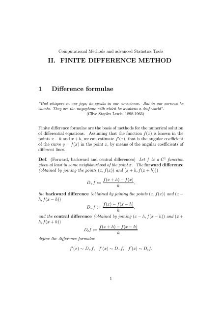
Def. (Forward, backward and central differences) Let f be a C 1 function
given al least in some neighbourhood of the point x. The forward difference
(obtained by joining the points (x, f(x)) and (x + h, f(x + h)))
D+f :=
f(x + h) ¡ f(x)
,
h
the backward difference (obtained by joining the points (x, f(x)) and (x ¡
h, f(x ¡ h))
f(x) ¡ f(x ¡ h)
D−f := ,
h
and the central difference (obtained by joining (x ¡ h, f(x ¡ h)) and (x +
h, f(x + h))
f(x + h) ¡ f(x ¡ h)
Dcf :=
h
define the difference formulae
f ′ (x) » D+f, f ′ (x) » D−f, f ′ (x) » Dcf.
1

By proceeding in analogous way, higher order derivatives can be approximated.
For example, approximating the function f by a second degree polynomial
through the points (x ¡ h, f(x ¡ h)), (x, f(x)) and (x + h, f(x + h)),
it turns out that D+(D−f) is a central difference approximation of f ′′ (x) :
= 1
h
[ 1
h
D+(D−f) = ( D−f(x + h) ¡ D−f(x)
h
1
(f(x + h) ¡ f(x)) ¡ (f(x) ¡ f(x ¡ h))] =
h
= 1
h 2 [f(x + h) ¡ 2f(x) + f(x ¡ h)] » f ′′ (x).
The study of the truncation error can be introduced by an example: if the
first derivative of the function e x is approximated by the forward (central)
difference operator in the point x = 1, the truncation errors D+e x ¡ e x ,
(Dce x ¡ e x ) for increments h, h/2, h/4,... are written in the following table.
The ratio between an approximation and the subsequent one is represented
by r:
h D+e x ¡ e x r Dce x ¡ e x r
0.4 0.624013 2.14 0.0730696 4.02
0.2 0.290893 2.06 0.0181581 4.00
0.1 0.140560 2.03 0.0045327 4.00
0.05 0.069103 2.01 0.0011327 4.00
0.025 0.034263 0.0002831
If the forward difference operator is applied, the error is approximately
halved when the increment is halved. If the case of central difference, the
error is approximately reduced by a factor 4 when h is halved. Such results
suggest that the errors behave linearly as h ! 0 in the first case, and
quadratically, O(h 2 ), in the other case.
Thm. II.1.1 (On truncation error)Let f be sufficiently regular and let ET
be its truncation error. Then ET = O(h) in case of a forward difference,
ET = O(h 2 ) in case of a central difference, as h ! 0. Besides, for the central
difference D+(D−) approximating f ′′ (x), the truncation error is O(h 2 ) as
h ! 0.
PROOF.
2

Let us apply Taylor’s formula. 1 If the function is twice continuously derivable,
ET :=
f(x + h) ¡ f(x)
h
¡ f ′ (x)
= 1
h (f(x) + hf ′ (x) + h2
2 f ′′ (ξ) ¡ f(x)) ¡ f ′ (x) = h
2 f ′′ (ξ)
where ξ is a suitable point of (x, x + h). If the function is C (3) then the
central difference approximation gives the truncation error
ET = 1
2h [f(x + h) ¡ f(x ¡ h)] ¡ f ′ (x)
= 1
2h [f(x)+hf ′ (x)+ h2
2 f ′′ (x)+ h3
6 f ′′′ (ξ1)¡f(x)+hf ′ (x)¡ h2
2 f ′′ (x)+ h3
6 f ′′′ (ξ2) ]
= 1
2h [h3
6 f ′′′ (ξ1) + h3
Finally, if f 2 C4 , we have
6 f ′′′ (ξ2)] = O(h 2 ). 4
D+(D−f) = 1
[f(x + h) ¡ 2f(x) + f(x ¡ h)]
h2 = 1
h 2 [f(x) + hf ′ (x) + h2
2 f ′′ (x) + h3
6 f (3) (x)+
+O(h 4 ) ¡ 2f(x) + f(x) ¡ hf ′ (x) + h2
2 f ′′ (x) ¡ h3
6 f (3) (x) + O(h 4 )] =
= 1 h2
[(h2 +
h2 2 2 )f ′′ (x) + O(h 4 )] = f ′′ (x) + O(h 2 ). 4
The influence of rounding errors in difference formulae for derivatives is
described in the following table, where each central difference is computed
for the function e x in x = 1. Computations were performed with precision
1 Recall Taylor’s formula: if f is C r+1 in some neighbourhod of x then the r¡th re-
mainder satisfies
f(x + h) ¡ [f(x) + hf ′ (x) + h2
2 f ′′ (x) + . . . + hr
r! f (r) (x)] = O(h r+1 ), as h ! 0.
Here the Landau’s symbol O(h m ) as h ! 0 denotes any infinitesimal fuction S(h) such
that S(h)/h m stays bounded as h ! 0. There are several explicit expression of the
remainder: for example if f 2 C r+1 there is ξ 2 [x, x + h], such that the r-th remainder
is equal to hr+1
(r+1)! f (r+1) (ξ) (if, say, h > 0).
3

ǫ = 2.22 £ 10 −16 . As h decreases, the global error is reduced till a certain
value of h, then it increases. Such a behaviour is due to the fact that the
values of e 1±h are computed approximately, and for small h cancellations take
place.
h Dce x ¡ e x
10 −1 0.004532
10 −2 0.000453
10 −3 0.0000000453
10 −4 0.00000000453
10 −8 -0.0000000165
10 −9 0.0000000740
10 −10 0.000000224
10¡14 -0.002172
Remark II.1A Let us denote by ˜ f(x§h) the approximate values of f(x§h)
and let us suppose that
j ˜ f(x § h) ¡ f(x § h)j · ǫ
where ǫ only depends on the precision of the used machine. Then, denoting
˜Dc the numerically computed central difference,
j ˜ Dcf(x) ¡ f ′ (x)j · j ˜ Dcf(x) ¡ Dcf(x)j + jDcf(x) ¡ f ′ (x)j · ǫ h2
+
h 6 f (3) (ξ)
The bound describes the real situation, there is a divergent component of
the error as h ! 0. In other words, for decreasing h rounding errors can
prevail on truncation error, with unreliable results. The situation is described
in Figure II.1. An optimal choice of h corresponds to the minimum of the
function ǫ
h
+ h2
6 max jf (3) j.
2 Finite difference method
Does science make the Creator superfluous? No. The sentence ”God created the
world” is not an outmoded scientific statement. It is a theological statement that is
concerned with the relation of the world to God. Being created is a lasting quality
in things and a fundamental truth about them. (YouCat 41)
4

errore(h)
errore totale
h
errore di troncamento
errore di arrotondamento
Figure 1: Rounding error and truncation error in the approximation of the derivative
by central differences
The difference method is based on the choice of subintervals [xi, xi+1] of
[a, b] and the approximation of derivatives by suitable difference operators.
We take equal intervals with length h = (b ¡ a)/n, so the subdivision points
are given by
xi = a + ih, i = 0, 1, ..., n
We denote f¯yi, i = 1, ..., ng the discrete approximation of the values y(xi)
of the continuos variable solution. Let us analyze the method in the case of
the linear problem
′′ ¡y (x) + q(x)y(x) = f(x), a < x < b
(1)
y(a) = α, y(b) = β
where q(x), f(x) are assigned functions, continuous in the interval [a, b].
Under the hypothesis
q(x) ¸ 0 (2)
existence and uniqueness of the solution can be proved for the problem (1).
Moreover, the solution is C 2 and any further regularity assumption on data
q(x), f(x) implies further regularity of the solution: for example, if f(x), q(x)
admit second derivative, the solution has the fourth derivative. At each node
xi, the derivative is discretized by means of the difference operator
y ′′ (xi) » y(xi+1) ¡ 2y(xi) + y(x(xi−1)
h2 .
5

Inserting such approximation in the equation (1) for i = 1, 2, . . . , n ¡ 1 and
replacing y(xi) by ¯yi, we obtain the following linear equations
or
¡ ¯yi+1 ¡ 2¯yi + ¯yi−1
h 2 + q(xi)¯yi = f(xi), i = 1, 2, . . . , n ¡ 1
¡¯yi+1 + ¯yi(2 + h 2 qi) ¡ ¯yi−1 = h 2 fi, i = 1, 2, . . . , n ¡ 1 (3)
where qi = q(xi), fi = f(xi). In particular, for i = 1 ad i = n ¡ 1, taking
into account the boundary conditions, we have the equations
for i = 1, (2 + h 2 q1)¯y1 ¡ ¯y2 = α + h 2 f1 (4)
for i = n ¡ 1, (2 + h 2 qn−1)¯yn−1 ¡ ¯yn−2 = β + h 2 fn−1 (5)
Thm. II.2.1 (Existence and uniqueness of the numerical solution)The difference
method applied to the problem (1) leads to a discrete problem which
is the linear system of n ¡ 1 equations
where
and
A =
⎛
⎜
⎝
A¯y = b (6)
¯y = (¯y1, . . . , ¯yn−2, ¯yn−1) T ,
(2 + h 2 q1) ¡1 0
¡1 (2 + h 2 q2) ¡1
.
.
.
¡1 (2 + h 2 qn−2) ¡1
0 ¡1 (2 + h 2 qn−1)
b = (h 2 f1 + α, h 2 f2, ..., h 2 fn−2, h 2 fn−1 + β) T .
Under the hypothesis q(x) ¸ 0 such a system admits a unique solution.
PROOF
Equations (3), (4), (5) can be written in vector form as stated. Now from
linear algebra
A is non-singular () z T Az 6= 0, 8z 6= (0, ..., 0).
6
.
.
⎞
⎟
⎠

By hypothesis (2), A satisfies:
z T Az ¸ (z1, ..., zn−1)
⎛
⎜
⎝
= (z1, ..., zn−1)
2 ¡1 0
¡1 2 ¡1
. . . . .
¡1 2 ¡1
0 ¡1 2
⎛
⎜
⎝
2z1 ¡ z2
¡z1 + 2z2 ¡ z3
.
¡zj−1 + 2zj ¡ zj+1
.
¡zn−2 + 2zn−1
⎞
⎟ ⎛ ⎞
⎟ z1 ⎟ ⎜ ⎟
⎟ ⎜ ⎟
⎟ ⎝ . ⎠
⎟
⎠ zn−1
= 2z 2 1 ¡ z1z2 ¡ z1z2 + 2z 2 2 ¡ z2z3 + ... ¡ zn−2zn−1 + 2z 2 n−1
⎞
⎟
⎠
= z 2 1 + (z1 ¡ z2) 2 + ... + (zn−2 ¡ zn−1) 2 + z 2 n−1
for any (z1, ..., zn−1) 6= (0, ..., 0). Thus A is positive definite, hence nonsingular:
then the discrete model is solvable under the same hypothesis of
the continuous variable one, and the statement is proved. 4
The discrete solution ¯yi, i = 0, 1, ..., n, depends on the discretization gauge h.
Then an important question is about the convergence problem as h ! 0:
is it possible to approximate the continuous solution, acording to a fixed
precision, for sufficiently small h? The approximation should be pointwise,
since the solution of the boundary value problem is continuous. The study
of convergence is introduced by the following example.
Example II.2A Let us consider the problem
¡y ′′ (x) + y(x) = 0, y(0) = 0, y(1) = sinh(1)
which admits tha analytic solution y(x) = sinh(x). For n = 4, i.e. h = 0.25,
the discrete problem consists in solving the system A¯y = b with unknown
(¯y1, ¯y2, ¯y3) and
A =
⎛
⎜
⎝
(2 + h 2 ) ¡1 0
¡1 (2 + h 2 ) ¡1
0 ¡1 (2 + h 2 )
7
⎞
⎟
⎠ ; b =
⎛
⎜
⎝
> 0
0
0
sinh(1)
⎞
⎟
⎠

The numerical computation can be performed by a program of the following
type (the language and environment R can be taken from CRAN, or www.Rproject.org)
programma

y
5 10 15 20 25
y’’+y=x^2, y(−1)=3, y(1)=5
−1.0 −0.5 0.0 0.5 1.0
Figure 2: The difference method applied to a problem y ′′ (x) + y(x) = x 2 , with
Dirichlet conditions y(a) = α, y(b) = β.
EX. II.2B - Let us consider the Dirichlet problem
y ′′ (x) + x 2 y(x) = sin(x)
y(¡4π) = 0, y(4π) = 0
It is solved by a difference scheme, building an R function with output in
Figure 4.
As the above table suggests, the following theorem shows that, if the solution
is sufficiently regular, the truncation error of the solution is O(h 2 ).
Thm. II.2.2 (Convergence) Let y(x) be the solution of the problem with
Dirichlet conditions
¡y ′′ (x) + q(x)y(x) = f(x), y(a) = α, y(b) = β
with q(x) and f(x) continuous functions on [a, b] and q(x) ¸ 0. Assume,
moreover, that the function y(x) has bounded fourth derivative, jy (4) (x)j · M
for any x 2 [a, b]. If the approximation of y(xi) obtained by the difference
method is denoted by ¯yi, then for some C independent of h,
jy(xi) ¡ ¯yij · Ch 2 , i = 1, 2, ..., n ¡ 1
9
x

y
0.0 0.1 0.2 0.3 0.4 0.5
−y’’+(x^2−1)y=0, y(−3)=e^(−9/2),y(−3)=e^(−9/2)
−3 −2 −1 0 1 2 3
Figure 3: The difference method applied to the harmonic oscillator ¡y ′′ (x)+(x 2 ¡
1)y(x) = 0 with Dirichlet conditions y(¡3) = y(3) = e −4.5 .
y
−0.3 −0.2 −0.1 0.0 0.1 0.2 0.3
x
y’’(x)+x^2y(x)=sin(x), y(−4*pi)=0, y(4*pi)=0
−10 −5 0 5 10
Figure 4: The difference method applied to the forced harmonic oscillator y ′′ (x)+
x 2 y(x) = sin(x) with Dirichlet conditions y(¡4π) = 0 , y(4π) = 0.
x
10

i.e. the method satisfies a convergence of order 2.
Concepts of the PROOF
Although we don’t give a complete proof, we can distingish two components
of the concept of convergence: consistence and stability. On one hand,
the quantity
τi = ¡ 1
h 2 [ u(xi+1) ¡ 2u(xi) + u(xi−1 ] + q(xi)y(xi) ¡ f(xi) (7)
is introduced. It represents the local discretization error: the error committed
in the node xi by the true solution when inserted in the discrete scheme.
By introducing the appropriate Taylor’s expansions, as in the proof of Thm.
II.1.1, we see that for some ξ
k τi k=k u ′′ (xi) + h2
12 u(4) (ξ) + q(xi)u(xi) ¡ f(xi) k=k h2
12 u(4) (ξ) k· Mh 2 /12. (8)
On the other hand, denoting by uh the vector of the approximation ( ¯yi ),
and by u the vector of the true values of the solution, the convegence regards
just the global error of the solution E := u ¡ uh. Now by the method uh
obeys the linear system
Auh = b.
Hence
Au ¡ Auh = Au ¡ b.
Now, the right hand side is just τ, the vector of local discretization errors τi
in (7), so that
A(u ¡ uh) = τ.
11

Since A is invertible, the error of the solution can be evaluated 2 in norm:
k E k=k A −1 τ k·k A −1 kk τ k (9)
To ensure convergence two facts have to be verified:
1) k τ k ! 0, for some norm: this property is the consistence of the
numerical method
2) k A −1 k· C, with C independent of h: this property is the stability
of the numerical method, it is verified if the matrix A −1 is not divergent in
norm as h ! 0.
If we choose, for example, the norm k w k:= maxi jwij, we have
k τ k= max jτij · Mh
i
2 /12 to 0 as h ! 0
by (8), whence consistence is proved. For what concerns stability, one must
prove that A is nonsingular uniformly with respect to h, for example by
showing that the lowest eigenvalue is larger than a positive constant independent
of h. That can be proved, the stability property holds, and the
convergence of the method follows. 4
3 Further applications of the difference method
The creation of the world is, so to speak, a ”community project” of the Trinitarian
God. The Father is the Creator, the Almighty, The Son is the meaning and heart of
2
In these evaluations, the norm of a vector can be the usual Euclidean norm (k w k=
w2 1 + . . . + w2 n ), or the simpler (and topologically equivalent) maximum norm: k w k:=
maxi jwij. The norm of a matrix is induced by the choice of the vector norm by the
definition
k Bv k
k B k:= sup
v=0 k v k .
If, for example, the maximum norm for vectors is chosen, the induced norm of a matrix
turns out to be the maximum among the sum of rows (in absolute value):
k B k= max
i
n
jbijj.
In any case, after choosing a vector norm and the induced matrix norm, it is guaranteed
that
k Bv k·k B k ¢ k v k, 8v.
12
j=1

the world: ”All things were created through him and for him” (Col 1:16). We find
out that the world is good for only when we come to know Christ and understand
that the world is heading for a destination: the truth, goodness and beauty of the
Lord. The Holy Spirit holds everything together: he is the one ”that gives life” (Jn
6,63).
Let us analyze the finite difference method applied to convection-diffusion
problems.
Ex.II.3A (Convection-diffusion problems with Dirichlet conditions)
¡y ′′ (x) + p(x)y ′ (x) + q(x)y(x) = f(x), a < x < b
y(a) = α, y(b) = β
where p(x), q(x), f(x) are continuous functions on [a, b] with q(x) ¸ 0. The
analytical problem turns out to admit a unique solution in the the class C 2 .
Setting h = (b¡a)/n, for given n 2 N, let us consider the following difference
scheme obained by use of central difference operators:
¡ ¯yi+1 ¡ 2¯yi + ¯yi−1
h2 + p(xi) ¯yi+1 ¡ ¯yi−1
+ q(xi)¯yi = f(xi)
2h
for i = 1, . . . , n ¡ 1. The boundary conditions are: ¯y◦ = α, ¯yn = β. The
discrete problem is equivalent to a linear system A¯y = f with a tridiagonal
coefficient matrix:
A =
⎛
⎜
⎝
(2 + h 2 q1) ¡1 + h
2 p1
.
.
Under the following hypothesis
.
.
¡1 ¡ h
2 pi (2 + h 2 qi) ¡1 + h
2 pi
.
.
.
.
¡1 ¡ h
2 pn−1 (2 + h 2 qn−1)
h
2 jp(xi)j < 1, i = 1, 2, ..., n ¡ 1 (10)
then the lower and upper diagonals are strictly less, in absolute value, than
the principal diagonal. Proceeding as in the proof of Thm. II.2.1, setting for
convenience 2+ǫ and ¡2 the diagonal and off-diagonal elements of a suitable
comparison matrix
⎛
z T Az ¸ z T
⎜
⎝
2 + ǫ ¡2
.
.
. . .
¡2 2 + ǫ ¡2
.
13
.
.
. .
¡2 2 + ǫ
⎞
⎟
⎠
z
.
.
⎞
⎟
⎠

y
0.0 0.1 0.2 0.3 0.4 0.5 0.6 0.7
y’’(x)+(3*x−2)*y’(x)+(x^2+1)*y(x)=cos(x/2), y(−6*pi)=0, y(6*pi)=0
−20 −10 0 10 20
Figure 5: The difference method applied to the the convection-diffusion problem
¡y ′′ (x)+(3x¡2)y ′ (x)+(x 2 +1)y(x) = cos(x/2) with Dirichlet conditions y(¡6π) =
0 , y(6π) = 0.
¸ ǫz 2 1 + (p 2z1 ¡ p 2z2) 2 + . . . + ( p 2zn−2 ¡ p 2zn−1) 2 + ǫz 2 n−1 ,
which is > 0 for any nonzero z 2 R n−1 . Hence we have the following result.
Thm. II.3.1 (Existence and uniqueness of solution of the discretized problem)
The discretized version of the convection-diffusion problem above described
admits a unique solution if h = (b ¡ a)/n is chosen sufficiently small
with respect to the convection term p(x), as in (10).
Ex.II.3B (Alternative discretizations are possible) The restriction (10) can
be eliminated by discretizing in another way the term p(x)y ′ . More precisely,
we set
¡ ¯yi+1 ¡ 2¯yi + ¯yi−1
h 2
¡ ¯yi+1 ¡ 2¯yi + ¯yi−1
h 2
+ p(xi) ¯yi+1 ¡ ¯yi
h
+ p(xi) ¯yi ¡ ¯yi−1
h
x
14
+ q(xi)¯yi = f(xi), if p(xi) · 0
+ q(xi)¯yi = f(xi), if p(xi) > 0

This scheme, which is known as upwind difference method, , may be written
in the form
¡ ¯yi+1 ¡ 2¯yi + ¯yi−1
h 2
¡ (jpij ¡ pi)¯yi+1 ¡ 2jpij¯yi + (jpij + pi)¯yi−1
2h
+ qi¯yi = fi
The upwind scheme is less accurate than the preceding one, but it is solvable
without restrictions on the choice of h. Indeed, the matrix of the corresponding
linear system turns out to be with diagonal predominance.
II.3.C NEWTON’S METHOD
In the scalar case with f 2 C (1) , f ′ (x) 6= 0, the solution of the equation
f(x) = 0 is approximated by a sequence xn starting from a (sufficiently
near) point x◦. The idea, at the k¡th step, is to replace the curve f by the
tangent line at xk, i.e. to solve the linear equation 0 = f(xk)+f ′ (xk)(x¡xk):
xk+1 = xk ¡ [f ′ (xk)] −1 f(xk).
In several dimensions suppose that f is regular with a non singular Jacobian
matrix :
f : R m ! R m , f 2 C 1 , J non singular.
Let us take an initial point x◦ sufficiently near the true solution of the equation
f(x) = 0.
At the k¡th step, the idea is to replace the function y = f(x) by its Taylor’s
formula at the first order, i.e. to solve the linear system 0 = f(xk)+J(xk)(x¡
xk), where J is the Jacobian:
xk+1 = xk ¡ [J(xk)] −1 f(xk).
Ex.II.3D (The difference method applied to a nonlinear problem)
y ′′ (x) = 1
2 (1 + x + y)3 , x 2 (0, 1)
y(0) = y(1) = 0
Setting f(x, y) := 1
2 (1 + x + y)3 , let’s notice that
∂f
∂y
= 3
2 (1 + x + y)2 ¸ 0
Then it can be shown that such a boundary value problem admits a unique
solution. Let us discretize the interval (0, 1) by the points xi = ih, with
15

h = 1/(n + 1) and i = 0, 1, ..., n + 1. Let us denote by ¯yi the values of
the approximated solution in the points xi. By discretizing y ′′ by means f
central differences, the following nonlinear system is got:
¯y◦ = 0, ¯yn+1 = 0
¡ ¯yi+1−2¯yi+¯yi−1
h 2
+ 1
2 (1 + xi + ¯yi) 3 = 0, (1 · i · n)
Eliminating the variables ¯y◦, ¯yn+1, the system can be written in the following
matrix form
with ¯y = (¯y1, ..., ¯yn) T and
A =
⎛
⎜
⎝
2 ¡1
¡1 2 ¡1
.
.
. . .
¡1 2 ¡1
¡1 2
A¯y + h 2 B(¯y) = 0 (11)
⎞
⎟
⎠
, B(¯y) = diag(f(xi, ¯yi)), i = 1, 2, ..., n
The nonlinear system (11) can be solved, for example, by Newton’s method.
Indeed, the Jacobian matrix of the system is given by
J = A + h 2 By
(12)
By virtue of the property fy ¸ 0, such a Jacobian turns out to be a matrix
with diagonal predominance and positive definite. Therefore the Newton’s
method is convergent if the initial values are chosen sufficiently near the
solution. The implementation of Newton’s method is the following. A
plausible initial point ¯y (◦) is chosen, the (r+1)¡th iterated vector is obtained
by solving the linear system
A + h 2
By
and setting
v = ¡A¯y (r) ¡ h 2 B(¯y (r) )
¯y (r+1) = ¯y (r) + v.
As it is easily verified, the exact solution of the continuous problem is y(x) =
¡ x ¡ 1.
2
2−x
By a program of the following type we obtain y (1) from an initial vector,
y (◦) = 0. By the same program we obtain y (2) from y (1) = 0... and so on:
16

iterabile

above consistence and stability, and using the fact that the nonlinear term
f(x, y) is monotonic.
Ex.II.3E (The difference method applied to a partial differential equation
) We already showed the solution of the heat equation on the line ¡1 <
x < +1 by using the convolution properties of the Fourier transform. Let
us show how to solve numerically the heat equation for x in some bouded
interval: the mixed problem (initial value and boundary value problem)
⎧
⎪⎨
⎪⎩
ut ¡ D uxx = 0
u(x, 0) = f(x)
u(0, t) = g1(t), u(0, t) = g2(t), 0 < t < T
(13)
where D is the diffusion coefficient, and f(x), g1(t), g2(t) are given functions.
Let us consider a discretization with nodes (xj, tn) , with xj = jh, tn = nk
and h = L/J, k = T/N. Let us denote by ūj,n the numeric solution in the
node (xj, tn). By the above initial condition
while the boundary conditions imply
ūj,0 = f(xj), j = 0, 1, ..., J
ū0,n = g1(tn), ūJ,n = g2(tn).
For 0 < j < J, n > 0 a possible discretization of (13) in the point (xj, tn) is
got by means of a forward difference for the derivative ut and by a central
difference for the second derivative uxx:
ut » ūj,n+1 ¡ ūj,n
, uxx »
k
ūj+1,n ¡ 2ūj,n + ūj−1,n
h2 By substituting in (13), we obtain the following relation for j = 1, ..., J ¡ 1,
and n = 0, ..., N ¡ 1
where
ūj,n+1 = (1 ¡ 2r)ūj,n + r(ūj+1,n + ūj−1,n
(14)
r = Dk/h 2 . (15)
The method is explicit: in xj the numerical solution ū at time tn+1 is
obtained from ū in the three points xj−1, xj, xj+1 at time tn, by an explicit
formula and not by solving a system. Hence in this case the existence of the
18

u
t
Figure 6: The explicit method (??) applied to the the diffusion mixed problem
(13). Here D=0.45, and L = T = J = N = 20, so Dk/h 2 · 1/2 and the explicit
method is convergent
u
t
Figure 7: The explicit method (14) applied to the the diffusion mixed problem
(13). Here D=0.55, and L = T = J = N = 20, so Dk/h 2 > 1/2 and the explicit
method is unstable.
19
x
x

u
x
Figure 8: The implicit method (18) applied to the the diffusion mixed problem
(13). Here D = 1, L = 80, T = 160, J = 40, N = 40. Athough Dk/h 2 > 1/2, the
implicit method is convergent.
numerical solution is obvious. However the convergence of ū to the analytic
solution u as h, k ! 0 is not always true. Indeed, in Figures II.6 and II.7,
with slightly different choice of parameters, we see different behaviours of the
numerical solution. Such a numerical example shows the importance of the
quantity (15). Actually one can prove that the condition
r = Dk/h 2 · 1
2
t
(16)
is a necessary condition for stability of the explicit numerical method. In
practice, it ensures a sufficiently high velocity of propagation of the discrete
signal. As for convergence, it is sufficient to remark that the explicit scheme
is consistent. More precisely, one can prove that, for a sufficiently regular
function, the local discretization error behaves like O(k + h 2 ). This implies
that the the scheme (14) is convergent (since it is stable and consistent) under
the condition (16). It is an example of conditionally convergent scheme.
Unconditionally convergent methods can be obtained using implicit schemes
where a linear system has to be solved at each time level tn. Such a scheme
can be obtained by using a backward difference, instead of a forward difference,
to approximate the derivatie ut. This way the differental equation (13)
20

is transformed into the difference equation:
whence
1
k (ūj,n ¡ ūj,n−1) ¡ D 1
h2 (ūj+1,n ¡ 2ūj,n + ūj−1,n) = 0 (17)
¡rūj−1,n + (1 + 2r)ūj,n ¡ rūj+1,n = ūj,n−1
(18)
for n = 1, 2, ..., Nad j = 1, 2, ..., J ¡ 1. Since the values ū0,n and ūJ,n are
determined by the boundary conditions, (18) is a system of equations in the
J ¡ 1 unknowns ū1,n, . . . , ūJ−1,n. The matrix of the system
⎛
⎜
⎝
1 + 2r ¡r . . . . . . . . .
. . . ¡r 1 + 2r ¡r . . .
. . . . . . . . . ¡r 1 + 2r
is symmetric and with diagonal predominance, as in the above discussed onedimensional
boundary problems. Therefore the matrix is positive definite
and the numerical solution exists.
The convergence problem, as usual, consists of two parts: consistence and
stability. The local discretization error τj,n is defined by the following relation
τj,n := ut(xj, t ¡ n) ¡ Duxx(xj, tn) ¡
ūj,n ¡ ūj,n−1
Thus by Taylor’s formula (Section I on difference formulae)
k
⎞
⎟
⎠
τj,n = 1
2 utt(xj, ¯tn)k ¡ D
12 uxxxx(¯xj, tn)h 2
¡ D ūj+1,n ¡ 2ūj,n + ūj−1,n
h2
.(19)
where ¯tn is a suitable point of the interval (tn−1, tn), and ¯xj 2 (xj−1, xj+1).
Therefore, if a solution is sufficiently regular,
τj,n = O(k) + O(h 2 ).
As for stability, defining the global error ej,n := uj,n ¡ ūj,n, one can prove
that
(1 + 2r)ej,n = ej,n−1 + r(ej+1,n + ej−1,n) ¡ kτj,n
Setting En = max0·j·J jej,nj and ˆτ = maxj,n jτj,nj, the global error can be
bounded by the following steps:
(1 + 2r)jej,nj · En−1 + 2rEn + kˆτ
21

Taking the maximum over 0 · j · J
wence, by recurrence
This last inequality says that
En · En−1 + kˆτ
En · E◦ + nkˆτ · T ˆτ.
juj,n ¡ ūj,nj · T ˆτ
that is the implicit scheme is stable. Then convergence follows from consistence.
4
4 The elements of R
Apart from the Cross there is no other ladder by which we may get to heaven.
(St. Rose of Lima, 1586-1617)
> x x
[1] 4
>
> y y
[1] 2 7 4 1 (lo scrive cosi’, ma e’ un vettore colonna)
> ls() elenca tutti gli oggetti nel workspace
[1] "x" "y"
> x*y prodotto elemento per elemento
[1] 8 28 16 4
> y*y prodotto elemento per elemento
[1] 4 49 16 1
> y^2 elevamento al quadrato el. per el.
[1] 4 49 16 1
22

t(y) trasposta del vettore colonna y
[,1] [,2] [,3] [,4]
[1,] 2 7 4 1
> t(y)%*%y %*% e’ il prodotto righe per colonne
[,1] (in questo caso: prodotto scalare)
[1,] 70
> y%*%t(y) -> z prodotto righe per colonne
> z
[,1] [,2] [,3] [,4]
[1,] 4 14 8 2
[2,] 14 49 28 7
[3,] 8 28 16 4
[4,] 2 7 4 1
> a a
[,1] [,2] [,3] [,4] [,5]
[1,] -5 -1 3 7 11
[2,] -4 0 4 8 12
[3,] -3 1 5 9 13
[4,] -2 2 6 10 14 (nota: assegna per colonne)
> t(a) trasposta
[,1] [,2] [,3] [,4]
[1,] -5 -4 -3 -2
[2,] -1 0 1 2
[3,] 3 4 5 6
[4,] 7 8 9 10
[5,] 11 12 13 14 (cosi’ ha assegnato per righe)
>
> u u
[1] 2 5 3
> sum(u)/length(u) media camponaria di u
[1] 3.333333
23

mean(u) media campionaria di u
[1] 3.333333
> sum((u-mean(u))^2)/(length(u)-1) varianza campionaria di u
[1] 2.333333
> var(u) varianza campionaria di u
[1] 2.333333
> v u sum((u-mean(u))*(v-mean(v))/(length(u)-1)) covarianza di u,v
[1] 5
> cov(u,v) covarianza di u,v
[1] 5
> zz zz
[1] 1.00 1.33 1.66 1.99 2.32 2.65 2.98 3.31 3.64 3.97
> n for (i in 1:n)
+ for (j in 1:n)
+ if (i==j) if(condizione) esegui else esegui
+ A[i,j] A
[,1] [,2] [,3] [,4] [,5]
[1,] 1 0 0 0 0
[2,] 0 1 0 0 0
[3,] 0 0 1 0 0
[4,] 0 0 0 1 0
[5,] 0 0 0 0 1
> getwd() di’qual e’ il work directory
[1] "C:/Programmi/R/R-2.3.1"
Nel direttorio di lavoro, con l’editor semplice
di "blocco note" scriviamo il file codice
chiamandolo "sinusoide,txt":
24

sinusoide source("sinusoide.txt")
> x plot(x,sinusoide(x,4),ty="l")
in blocco note scrivo "tabella.txt"
peso altezza cibo
1 20 70 10
2 15 60 5
3 17 50 8
4 23 67 12
5 25 58 18
> read.table("tabella.txt")
peso altezza cibo
1 20 70 10
2 15 60 5
3 17 50 8
4 23 67 12
5 25 58 18
in workspace la leggo con "read.table"
> T x y z M M (3 colonne: cioe’ 3 variabili)
[,1] [,2] [,3] (5 righe: cioe’ 5 unita’ osservate)
25

[1,] 20 70 10
[2,] 15 60 5
[3,] 17 50 8
[4,] 23 67 12
[5,] 25 58 18
> media media
[1] 20.0 61.0 10.6
> var(M) matrice di covarianza
[,1] [,2] [,3] dei dati campionari della matrice M
[1,] 17.00 10.25 19.25 cioe’: cov(colonna i di M, colonna j di M)
[2,] 10.25 62.00 3.75 per i,j = 1,2,3
[3,] 19.25 3.75 23.80
> pnorm(2.3, mean=0, sd=1) funz. distribuzione N(0;1) in 2.3
[1] 0.9892759
> pnorm(5.8, mean=2, sd=3) funz. distribuzione N(2;9) in 5.8
[1] 0.8973627
> qnorm(0.897,mean=2, sd=3) quantile 0.897 di N(2;9)
[1] 5.793923
> dnorm(2.7,mean=0,sd=5) funz.densita’ N(0;25) in 2.7
[1] 0.0689636
> x hist(x) istogramma dei dati campionari x
> dbinom(10,size=22,prob=3/7) funzione di probabilita’, calcolata in 10,
[1] 0.1638484 di Binomiale (n=22, p=3/7)
> pbinom(10,size=22,prob=3/7) funzione distribuzione, calcolata in 10,
[1] 0.6802406 della stessa Binomiale
> qbinom(0.68,size=22,prob=3/7) quantile 0.68 di Binomiale (n=22, p=3/7)
[1] 10
> qt(0.95,df=13) quantile 0.95 di "t" di Student
[1] 1.770933 (con 13 gradi di liberta’)
26

qchisq(0.99,df=10) quantile 0.99 di "chi quadro"
[1] 23.20925 (con 10 gradi di liberta’)
-----------------------------------------
# codice di -y’’(x)+y(x)=0, y(a)=ya,y(b)=yb, con n passi
finite

finiteconvdiff

______________________________________________________
# codice di figura II6 (con D=0.45, L=T=J=N=20) schema alle differenze esplicito sta
# e di figura II7 (con D=0.55,L=T=J=N=20) schema esplicito instabile perche Dk/h^2 >
pdeII7

for (ii in 1:J-1)
for (jj in 1:J-1)
{
if (ii==jj)
A[ii,jj]