Windows QTL Cartographer 2.5 - FTP Directory Listing

Windows QTL Cartographer 2.5 

User Manual 

© 2010 N.C. State University, Bioinformatics Research Center

I 


Table of Contents 

About Windows QTL Cartographer 1 

WinQTLCart ................................................................................................................................... features 

1 

Compatible ................................................................................................................................... programs and formats 

1 

System ................................................................................................................................... requirements 

2 

Installing, ................................................................................................................................... uninstalling, upgrading 

2 

Using WinQTL - a high-level overview 2 

When to ................................................................................................................................... use WinQTLCart 

4 

WinQTLCart Windows & Menus 4 

Main window ................................................................................................................................... - Menus 

4 

Main w indow - .......................................................................................................................................................... Menus - File 

4 

Main w indow - .......................................................................................................................................................... Menus - Edit 

5 

Main w indow - .......................................................................................................................................................... Menus - View 

5 

Main w indow - .......................................................................................................................................................... Menus - Method 

5 

Main w indow - .......................................................................................................................................................... Menus - Tools 

6 

Main w indow - .......................................................................................................................................................... Menus - Help 

7 

Chromosome ................................................................................................................................... graph display - Menus 

7 

Chromosome .......................................................................................................................................................... graph - Menus - File 

7 

Chromosome .......................................................................................................................................................... graph - Menus - View 

7 

Chromosome .......................................................................................................................................................... graph - Menus - Setting 

8 

Main window ................................................................................................................................... tour 

9 

Main w indow .......................................................................................................................................................... - Tree Pane 

10 

Main w indow .......................................................................................................................................................... - Form Pane 

12 

Main w indow .......................................................................................................................................................... - Data Pane 

12 

Graph ................................................................................................................................... window - Menus 

12 

Graph w indow .......................................................................................................................................................... - Menus - File 

13 

Graph w indow .......................................................................................................................................................... - Menus - Chrom 

13 

Graph w indow .......................................................................................................................................................... - Menus - Traits 

14 

Graph w indow .......................................................................................................................................................... - Menus - Effects 

14 

Graph w indow .......................................................................................................................................................... - Menus - Tools 

15 

Graph w indow .......................................................................................................................................................... - Menus - Setting 

15 

One-page ................................................................................................................................... display window - Menus 

16 

One-Page w indow .......................................................................................................................................................... - Menus - File 

16 

One-Page w indow .......................................................................................................................................................... - Menus - View 

16 

One-Page w indow .......................................................................................................................................................... - Menus - Setting 

17 

Graph ................................................................................................................................... window - Procedures 

17 

Tracing coordinates .......................................................................................................................................................... on the graph 

19 

Selecting traits .......................................................................................................................................................... for graph display 

20 

Selecting chromosomes .......................................................................................................................................................... for graph display 

21 

Setting display .......................................................................................................................................................... parameters 

21 

Setting a test .......................................................................................................................................................... hypothesis 

23 

Show ing QTL .......................................................................................................................................................... information 

24 


Contents 

WinQTLCart Procedures 25 

Setting ................................................................................................................................... the working directory 

25 

Importing ................................................................................................................................... and exporting 

25 

Importing files .......................................................................................................................................................... 25 

Exporting source .......................................................................................................................................................... data and results 

29 

Exporting source ......................................................................................................................................................... data to QTL Cartographer 

30 

Exporting source ......................................................................................................................................................... data to an MCD file 

30 

Exporting results ......................................................................................................................................................... from the Graph w indow 

31 

Working ................................................................................................................................... with source data files 

31 

Opening source .......................................................................................................................................................... data files 

32 

Working w ith .......................................................................................................................................................... a source file's marker genotype data 

32 

Working w ith .......................................................................................................................................................... a source file's traits values 

33 

Working w ith .......................................................................................................................................................... a source file's basic information 

34 

Working w ith .......................................................................................................................................................... source file's individual information 

35 

Working w ith .......................................................................................................................................................... source file's chromosome information 

37 

Working w ith .......................................................................................................................................................... source file's trait information 

38 

Working w ith .......................................................................................................................................................... source file's other trait information 

39 

MCD file format .......................................................................................................................................................... 39 

Creating ................................................................................................................................... a new source data file from raw data 

44 

Creating ................................................................................................................................... simulation data 

51 

Single-marker ................................................................................................................................... analysis 

55 

Setting ................................................................................................................................... threshold levels (IM & CIM) 

56 

Setting threshold .......................................................................................................................................................... levels manually 

57 

Setting threshold .......................................................................................................................................................... levels via permutations 

57 

Interval ................................................................................................................................... Mapping 

58 

Running interval .......................................................................................................................................................... mapping analysis 

58 

Composite ................................................................................................................................... Interval Mapping 

60 

Running composite .......................................................................................................................................................... interval mapping analysis 

60 

Multiple ................................................................................................................................... Interval Mapping 

63 

About the MIM .......................................................................................................................................................... form 

63 

Creating MIM .......................................................................................................................................................... initial model 

65 

Regression ......................................................................................................................................................... options 

66 

CIM search ......................................................................................................................................................... option 

68 

MIM search ......................................................................................................................................................... option 

69 

Refining the MIM .......................................................................................................................................................... model 

70 

Multiple-trait ................................................................................................................................... MIM 

72 

About the Mt-MIM .......................................................................................................................................................... form 

72 

Mt-MIM Control .......................................................................................................................................................... File 

74 

Mt-MIM Functions .......................................................................................................................................................... 75 

Bayesian ................................................................................................................................... Interval Mapping 

76 

Running Bayesian .......................................................................................................................................................... interval mapping analysis 

77 

Multiple-trait ................................................................................................................................... analysis 

78 

Drawing ................................................................................................................................... a chromosome tree 

78 

Adding QTL positions .......................................................................................................................................................... to the chromosome graphics 

80 

Tutorials 81 

Import ................................................................................................................................... data files 

81 

© 2010 N.C. State University, Bioinformatics Research Center 

II 

II

III 


Import data - INP .......................................................................................................................................................... format 

81 

Using Emap function .......................................................................................................................................................... 81 

Import data - OUT .......................................................................................................................................................... format 

81 

Import data - MapMaker .......................................................................................................................................................... format 

82 

Import data - Excel .......................................................................................................................................................... format 

82 

Import data - CSV .......................................................................................................................................................... format 

82 

Simulation ................................................................................................................................... source data file 

82 

Create ................................................................................................................................... new source data file 

83 

Single ................................................................................................................................... marker analysis 

83 

Interval ................................................................................................................................... mapping 

84 

Composite ................................................................................................................................... interval mapping 

84 

Multiple-trait ................................................................................................................................... analysis 

84 

Multiple ................................................................................................................................... Interval Mapping 

84 

Bayesian ................................................................................................................................... interval mapping 

85 

Result ................................................................................................................................... manipulation 

85 

Technical notes 85 

Troubleshooting ................................................................................................................................... 85 

1. Errors even .......................................................................................................................................................... to run Single Marker Analysis 

85 

2. Why my trait .......................................................................................................................................................... values are truncated into integers 

86 

3. WinQTLCart .......................................................................................................................................................... cannot import Map information from selected file 

86 

4. Invalid file or .......................................................................................................................................................... w rong format messages 

86 

5. Failures w hen .......................................................................................................................................................... I try to creat MCD file from text files 

86 

Technical ................................................................................................................................... Support 

86 

Credits ................................................................................................................................... & acknowledgements 

87 

Index 88 


About Windows QTL Cartographer 

WinQTLCart features 


About Windows QTL Cartographer 1 

Windows QTL Cartographer maps quantitative trait loci (QTL) in cross populations from inbred lines. 

WinQTLCart includes a powerful graphic tool for presenting mapping results and can import and export 

data in a variety of formats. 

WinQTLCart incorporates many of the modules found in its command-line sibling, QTL Cartographer, and 

provides a graphical interface to many of QTL Cartographer's features. 

WinQTLCart implements the following statistical methods: 

Single-marker analysis 55 

Interval mapping 58 

Composite interval mapping 60 

Bayesian interval mapping 76 

Multiple interval mapping 63 

Multiple trait analysis 78 

Multiple trait MIM analysis 78 

Features 

Supports various QTL mapping methods 

View, copy, and print graphs 

Includes an interface to help you build a source data file that WinQTLCart can use for analysis 

Import 25 data from Mapmaker / QTL and Microsoft Excel and CSV formats 

Export 29 graph data to Windows Excel format 

View, copy, and print chromosome information 78 graphically 

Produce a simulation 51 

data file 

Compatible programs and formats 

WinQTLCart can import and export data files in a variety of formats. 

Import success depends on the data file's format. Some data may need to be formatted manually before 

WinQTLCart can import it. 

Applications Formats Supported Import Export 

MapMaker/QTL .MAP – Map file 

.MPS – Map file 

.RAW – Cross data file 

Microsoft Excel .XLS X X 

Microsoft CSV .CSV X 

QTL Cartographer .INP – Map and Cross data files 

.MAP – Map file 

.CRO – Cross data file 

X 

X X 

WinQTLCart .MCD – Source data file X X

2 


Related topics 

Creating a new source data file 44 

Troubleshooting import errors 86 

Importing files 25 

Exporting source data and results 

System requirements 

WinQTLCart can run on the following operating systems: Windows 95, 98, ME, NT, 2000, XP and 

Windows 7. 

Because some WinQTLCart windows are quite large, the suggested minimum monitor resolution is 

1024x768. 

20MB free disk space for program files. 

512MB RAM. 

Any mouse or pointing device supported by Windows. 

Installing, uninstalling, upgrading 

Installing 

To install, double-click the WQTLSetup.exe file and follow the prompts. The default install directory is C: 

\NCSU\WinQTLCart2.5, though you can specify a different directory. 

The installer places a shortcut to the Windows QTL Cartographer program on your PC's Desktop, 

labeled WinQTLCart. Double-click the icon to run the program. 

Uninstalling 

To uninstall, run the Add/Remove Programs control panel and select Windows QTL Cartographer from 

the installed programs list. 

Upgrading 

If you have a prior version of WinQTLCart already on your PC, simply run the installer program. 

Upgrading to a new version of WinQTLCart does not overwrite your working files. However, the upgrade 

will replace the sample files that are part of the WinQTLCart distribution. 

Note 

You should close current running version of WinQTLCart first before installing the upgrading version. 

Using WinQTL - a high-level overview 

29 

Your goals in using WinQTLCart may include preparing data for publication or continued research into 

possible QTL sites. 

Step 1—Preparing your source data 

Your data files may come from another program or they may exist as raw data files. For WinQTLCart to 

work with your files, they need to conform to the program's .MCD file format 39 

. Review that file, as well 

as the other files included in the WinQTLCart distribution, such as the .QRT, .QPE, and other files. 


These are all text files that you can view in any text editor. 


Using WinQTL - a high-level overview 3 

Or, you may not have any data files or any data ready for import. You may instead want to use 

WinQTLCart to create simulation data to try out some hypotheses to view potential results. 

See these topics for more information: MCD file format 39 , Creating a new source data file from raw 

data 44 , Creating simulation data 51 

Step 2—Bringing data into WinQTLCart 

WinQTLCart can import map and cross data files from MapMaker/QTL, QTL Cartographer, and Microsoft 

Excel. As part of the import, WinQTLCart runs verification checks against the data. If the data does not 

conform to the accepted format, WinQTLCart displays an error message that should indicate the source 

of the problem. 

See these topics for more information: Importing files 25 , WinQTLCart cannot import Map information 

from selected file 86 , Invalid file or wrong format messages 86 

Your source data may not have come from another program, but may instead exist as raw source files. 

In that case, using WinQTLCart's Create a New Source File command steps you through all of the steps 

needed to translate the raw data into a readable form. The new source file will conform to WinQTLCart's 

MCD file format. 

See these topics for more information: Creating a new source data file from raw data 44 , MCD file 

format 39 

Step 3—Analyzing data using QTL Mapping Methods 

With WinQTLCart able to view the data, you can then select any of seven different analysis methods. 

The end result for some of these methods is another MCD file, but in most cases the process will create 

a .QRT result file that WinQTLCart can use to graph QTL information. 

See these topics for more information: Single-marker analysis 55 , Interval Mapping 58 , Composite 

Interval Mapping 60 , Multiple Interval Mapping 63 , Bayesian Interval Mapping 76 , Multiple-trait 

Analysis 63 , Multiple-trait MIM. 

Step 4—Viewing results and graphs 

WinQTLCart can present your data in graphics suitable for publication. You can show all chromosomes 

and their intervals in one display, while the Graph window display offers many parameters to help you 

fine-tune the visualization. 

See these topics for more information: Drawing a chromosome tree , Graph Window tour 

78 17 

Step 5—Saving and exporting results 

You can save your source data in .MCD format and your results files in .QRT format so you can work 

with them later in WinQTLCart. You can also export your results to other selected formats. 

See these topics for more information: Exporting source data and results 29 , Exporting results from the 

Graph window 31 , Exporting source data to an MCD file 30 , Exporting source data to QTL Cartographer 

30

4 


When to use WinQTLCart 

You can use WinQTLCart for any kind of data that is cross populations from inbred lines. WinQTLCart is 

a particularly powerful tool when you want to explore your results graphically. 

Prior to doing experiments, you could use WinQTLCart to explore some "what-if" scenarios in planning 

your experimental design. In WinQTLCart, you can create simulation data and then vary parameters 

setting to explore various QTL models. 

However, if you're working on a repetitive task that would be better off scripted, you may want to turn to 

QTL Cartographer, WinQTLCart's command-line sibling. For example, if you have expression data with 

thousands of features, you might want to run interval mapping on each feature, which would take a long 

time. This task can be automated via a shell script and made to run overnight. The results can then be 

imported into WinQTLCart and its graphs charted. 

WinQTLCart Windows & Menus 

Main window - Menus 

Menus in Main window include File 4 , Edit 5 , View 5 , Method 5 , Tools 6 , and Help 7 . 

Main window - Menus - File 

Icon Command Shortcut Key Function 

New... Ctrl + N Create a new source data file from raw text files. 

See Creating a new source data file 44 

Open... Ctrl + O Open a data file, result file or text file. 

Source data files you can open in WinQTLCart have the . 

MCD extension. Results files have the .QRT extension. 

Files with any other extension are opened as text files. 

Close Close the currently selected file. (The currently selected . 

MCD file's name is in the title bar and highlighted in the 

Tree pane). 

Save As... Save the currently active source data to a file with mcd 

format or a file with Microsoft Excel format. 

Import... Ctrl + I Import files in a variety of formats. See the importing files 

25 topic 

Simulation... Opens the Simulate Data dialog. See creating a 

simulation data file 51 

Export... Export the selected file to a different format. See Exporting 

source data and results 29 




Print... Ctrl + P Print the selected file in data pane. 

Print Setup... Opens Windows' Print Setup dialog box. 

Recently used 

files 

Main window - Menus - Edit 

WinQTLCart displays the last 6 data files you've worked 

with. 

Exit Closes WinQTLCart. 

If you have unsaved data, you'll be prompted to save it. 

Command Shortcut Key Function 

Copy Ctrl + C Copy selected text in Data pane 12 to the Windows clipboard. 

Select All Ctrl + A Click in the Data pane 12 and then choose this command to select all text 

in the data pane. Enables you to easily select and copy the text to a 

separate file. 

Main window - Menus - View 

Icon Command Shortcut Key Function 

Main window - Menus - Method 

Data Summary Summarizes statistical information of active source 

data file and displays in Text window. 

Result Graph... Ctrl + G View result file in the Graph window. See Graph Window 

tour 17 

Toolbar Select to toggle the Toolbar display. 

Status bar Select to toggle the Status bar display. 

Icon Command Function 

Single Marker Analysis... Displays the Single Marker Analysis 55 

form.

6 


Main window - Menus - Tools 

Interval Mapping... Displays the Interval Mapping 58 form. 

Composite Interval Mapping... Displays the Composite Interval Mapping form 60 . 

Multiple Interval Mapping... Displays the Multiple Interval Mapping 63 form. 

Click "OK" button to start MIM analysis and click 

"MtMIM" button to choose multiple-trait MIM 

analysis. 

Multiple Trait MIM Analysis... Display the Multiple Trait MIM Analysis form. 

Multiple Traits IM-CIM Analysis... Displays the Multiple Trait Analysis 78 form. 

Category Trait Analysis... Displays the Category Trait Analysis form. 

Bayesian Interval Mapping... Displays the Bayesian Interval Mapping 76 form. 

eQTL MIM Analysis... Displays the eQTL MIM Analysis form. 

Icon Command Shortcut 

Key 

Function 

Set Working directory... Set the default working directory. See Setting the 

working directory 25 

Draw chromosome graph... Show and print graphic displays of chromosomes 

from the Current active .MCD file. See Drawing a 

chromosome tree 78 

Copy between trait and 

otrait... 

Delete markers of same 

position... 

Notepad... Ctrl + Shift + 

N 

Calculator... Ctrl + Shift + 

C 

Copy normal trait to Other trait (category trait) or vise 

verse. 

Delete markers that have the same position in a 

chromosome and only keep one marker. 

Opens Notepad. Use Notepad as a convenient text 

editor to help format source data files. 

Open the Windows Calculator accessory. 


Main window - Menus - Help 

Icon Command Function 



About WinQTLCart Display About dialog of WinQTLCart. You can open 

WinQTLCart upgrade site in this dialog. 

Chromosome graph display - Menus 

Open a mcd source data file. From the Main window, select Tools>DrawChrom or click to draw 

the trees of chromosome graph 78 and markers in a single large window that is suitable for copying to 

an image program for later editing or printing and publication. 

Menus in Chromosome graph display window include File 

that will Copy content in window to the clipboard. 

7 , View 7 , Setting 8 

, and Copy_Graph 

Chromosome graph - Menus - File 

Command Function 

Copy to Clipboard Copies content in window to the clipboard. 

Print Graph… Print the graph. 

Exit Close the window and return to the Main window. 

Chromosome graph - Menus - View 


Proportion of Marker Number Show length of chromosome graph in proportion of marker number 

Proportion of Chromosome 

Len 

Show length of chromosome graph in proportion of chromosome length 

in cM 

Next Page >> Show next page of the graph if there are multiple pages. 

First Page Show First page of the graph. 

Add QTL Positions... Display QTL positions in the graph.

8 


Chromosome graph - Menus - Setting 


Select Chromosomes Select chromosomes to be showed in graph. 

Show Chromosome Name Toggle display between chromosome names or chromosome 

labels produced by WinQTLCart. 

Font Size >> Increase font size of graph. 

Font Size > Increase space between chromosomes. 

Space Between > Increase font size of chromosome names. 

Chromosome Name > Increase the number of chromosome displayed horizontally. 

Column Number

Main window tour 



When you start up Windows QTL cartographer, the program's Main window displays. 

From top to bottom, here's what you see: 

1. Title bar. Shows the name of the selected source data file. 

2. Menu bar 4 . 

3. Toolbar with one-click access to the program's major functions. Hover the pointer over a button to 

see a brief description of that command. The button's function is also described in the Status bar at 

the bottom of the window. 

4. Tree pane 10 for file management. Lists open files and organizes files under various category 

names (Source Files, Text Files, Results Files). 

5. Form pane 12 for displaying and controlling analysis of source data files. The form pane contents 

change based on the analysis method you select. 

6. Data pane 12 

for displaying data of currently selected file. 

7. The Status bar displays a variety of system messages; select View>Status bar to toggle its 

display. Click on each node in the tree pane or hover the pointer over a toolbar button or menu 

command to see the displayed message. The right area of the status bar also displays the current 

date and time, and also displays CAP, NUM, or SCRL if the Caps Lock, Num Lock, or Scroll Lock 

keys have been pressed. 

Double-click on a category name in the Tree pane to open files of that type. 

Left-click on a .MCD filename to make that the active source data file on which to run an

10 


Main window - Tree Pane 

analysis. 

Right-click on a filename to see appropriate commands for that file. 

The Main Window's Tree pane allows you to manage open files. The following table describes the many 

different options available via left-click, right-click, and double-click operations. 

Source file selected with right-click options displayed 

Tree Item Action Function 

Message window Left-click Displays WinQTLCart startup message in the data 

pane. 


Source files root Double-click Open a source data file (.MCD) 

Right-click>Open a File Open a source data file (.MCD) 


Result files root Double-click Open a result file (.QRT) 

Right-click>Open File Open a result file 


Text files root Double-click Open a text file (.TXT). 

Right-click>Open File Open a text file 





.MCD file Left-click Show file contents in the Data pane and set as current 

working .MCD file 

Double-click Open the .MCD file in Notepad 

Right-click options… 

>Open File Open a new source data file 

>Open with Notepad Open the .MCD file in Notepad 

>Refresh Re-load the file after modification 

>Single Marker Start single marker analysis 

>Interval Mapping Start interval mapping 

>Composite IM Start composite interval mapping 

>Multiple Traits Start multiple traits analysis 

>Multiple IM Start multiple interval mapping 

>Bayesian IM Start Bayesian interval mapping 


.QRT file Left-click Show this result file in text format via the Data pane 12 . 

Double-click Open the QRT file in the Graph window 


>Open File Open a new result file 

>Open with Notepad Open the .QRT file with Notepad 


>Close File Close the result file 

>Graphic Dialog Open the .QRT file in the Graph window 


.TXT file Left-click Show this text file in the Data pane 

Double-click Open the text file with Notepad 


>Open File Open a new text file 

>Open with Notepad Open the .TXT file with Notepad 


>Close File Close the text file. 

12 

17

12 


Main window - Form Pane 

The Form pane is the control panel you use to analyze your source data. It serves as a dashboard that 

presents a lot of information about your source data file at a glance. (The Form pane is keyed to the . 

MCD source data file only; it does not show information for any other file format.) 

This "control panel" changes based on the analysis method you select. For each analysis method, 

WinQTLCart displays different parameters and controls that help you control the analysis. 

When you first open WinQTLCart, you see the standard Source Data File Information form. Most of the 

options are disabled because no source data file has been loaded. Select an analysis method from the 

drop down list in the Analysis box on the right to begin working with the data. 

When you have opened a file, WinQTLCart enables the buttons and controls on the Source Data File 

Information form. These enable you to perform some basic manipulations to the source data (such as 

add traits, map information, etc.) 

Forms and disabled commands 

When you select an analysis method, WinQTLCart assumes you want to keep working with that method 

until you save your data or cancel the analysis. If you select the Interval Mapping (IM) method, 

WinQTLCart disables several toolbar and menu commands (such as the other analysis methods, setting 

the working directory, and so on). You need to either save your data or press the Cancel button on the 

IM form to leave the IM analysis mode. Leaving an analysis method re-displays the Source Data File 

Information pane. 

See the Source data file information 31 topic and the topics for each analysis method for the appropriate 

screen shot relevant to that method. 

Main window - Data Pane 

The large pane under the Form pane 12 displays the content of the active data or results file in text 

format. You cannot edit the displayed information from this pane. However, you can select the text with 

your cursor and copy the selected text to the clipboard. 

For .MCD source data files, WinQTLCart color-codes the data so you can easily determine what are 

comments, labels, headers, and so on. 

Graph window - Menus 

From the Main window, select View>Visualize Result to display the result file (*.qrt) in result graph 

window. 

Menus in Graph window include File 13 , Chrom 13 , Traits 14 , Effects 14 , Tools 15 , and Setting 15 

. 

In addition to the toolbar and menu commands, some functions are available by right-clicking on the 

graph. 


Graph window - Menus - File 




Open QTL Result File... Open a result file. Files with the .QRT extension are considered result 

files. 

Add QTL Result Graph... Adds a new graph to the current display. Files with the .QRT extension are 

considered result files. 

Note: The added result file should have same chromosome number and 

marker number as original one. You could add more than one new graph. 

Copy Graphic to 

Clipboard 

Copies the graph to the Windows clipboard. 

Save As New Name... Save the file under a different name in .QRT format. You may want to do 

this if you plan to work with the results in a later WinQTLCart session. 

Save As Text File... Save the results as a text file. You may want to do this if you plan to use 

the text file in another program. 

Save As Excel File... Save the data as an Excel file. Use Excel's charting capabilities to draw 

the graph. 

Save As EQTL File.. Save the data as the EQTL format that is used on Command-line version 

of QTL Cartographer. 

Print Graph... Print the graph to a selected printer. 

Exit Closes the Graph window. If you have unsaved data, you'll be prompted to 

save it. 

Graph window - Menus - Chrom

14 



Next Chrom >> Display the next chromosome in the file. 

Prev Chrom > Display the next trait in the file. 

Prev Trait

Graph window - Menus - Tools 




Display One Page Format... Show the graph information in a smaller, one-page format, for 

publication purposes. See One-page display window - Menus 

16 for more information. 

Show QTLs information... Display QTL information from a simulation parameter file or 

summary QTL peaks. See Showing QTL information 24 . 

Graph window - Menus - Setting 


Set Display Parameters… Allows you to customize the graph display. See Setting display 

parameters 21 . 

Set Test Hypothesis… Display result of different tests, such as H1:H3. See Setting a test 

hypothesis. 23 

Show Graph in LR/LOD 

Scale 

Show Black and White 

Graph 

Toggles between LR and LOD scale displays. Look for LR or LOD at 

the top of the y-axis line. 

Toggle between color and black-and-white display. Use black-andwhite 

graphs for publication. 

Show Colorful Background Activate a color or white background; might be useful for printing or to 

provide better contrast for color graph lines. 

Hide/Show Threshold Lines Toggle display. 

Show Horizontal Grids Toggle display. 

Show Vertical Grids Toggle display. 

Show Trait Names or 

Legend 

Show Marker Names Toggle display. 

Show Chromosome Names Toggle display. 

Toggle display. If traits are present, WinQTLCart defaults to showing 

legends on the right side of the graph. Use Set Display Parameters 

21 

to switch the legends to above the graph. 

Turn the trait name display on when you're loading more than one 

result file into a graph.

16 


Trace Coordinate in Graph Provides coordinates for a specific point on the graph. See Tracing 

coordinates on the graph 19 . 

One-page display window - Menus 

From the Graph window, select Tools>Display One Page Format to display the graphs in a single, large, 

scrolling window that is suitable for copying to an image program for later editing or printing for 

publication. 

The chromosomes and traits shown in the one-page display depends on the Select Chroms 21 and 

Select Traits 20 settings in the Graph window. 

Menus in One-page display window include File 16 , View 16 , Setting 17 

, and Copy_Graph that will 

Copy content in window to the clipboard. 

One-Page window - Menus - File 


Copy to Clipboard Copies content in window to the clipboard. 

Print Graph… Print the graph. 

Quit Close the window and return to the Graph window. 

One-Page window - Menus - View 


Show Frame Puts a border around the graph(s). 

LR Proportion Graph heights according to LR values. 

Show Color Graphic Toggle display of colors (axis lines remain black). 

Show Threshold Line Toggle display of threshold line. 

Show Marker Number Toggle display of marker numbers. 

Row Number>> Increase graph number in a row by 1. 


Row Number> Increase graph number in a column by 1. 

Column Number> Increase horizontal space between chromosomes. 

HSpace Between > Increase vertical space between chromosomes. 

VSpace Between > Increase title size. 

Title Font Size

18 


From top to bottom, here's what you see: 

1. Title bar. Shows the name of the selected results data file. You can have multiple results files 

loaded and multiple Graph windows open at a time. 

2. Menu bar 

12 

3. Toolbar with one-click access to the program's major functions. Hover the pointer over a button to 

see a brief description of that command. 

4. The large graph charts the data as a LOD (or LR) score profile. The higher the LOD, the greater the 

evidence for a QTL. 

5. The smaller graph at the bottom is the QTL effects window, showing additive or dominant effects or 

R2 or TR2 or S values. 

Graph window tips 

You can add several result files so they display at the same time on the current graph. You might 

want to run your data through the IM, CIM, and MIM analysis methods, for example, and then pull 

them all into the same graph to see how they compare. 

Peaks above the threshold line indicate a QTL. 

A high LOD value on the graph indicates a good QTL candidate. 

Right-click on the graph to see appropriate commands. (Commands described in the Graph window- 

Menus 12 

topic.) 

You can minimize the Graph window to the bottom of the Main window; a small bit of the title bar is 

visible. 

You can have the same result file open in several windows at the same time. This might be useful if 

you're testing various viewing parameters. To do this, minimize the current Graph window, go back 

to the Main window, ensure the result file is still active, and click the Graph toolbar button. 



Graph Window - Menus 12 

Tracing coordinates on the graph 19 

Selecting traits for graph display 20 

Selecting chromosomes for graph display 

Setting display parameters 

Setting a test hypothesis 

Showing QTL information 

Tracing coordinates on the graph 



Select Settings>Trace Coordinate in Graphic or click . As you move the cursor around the screen, 

note that the graph coordinates are displayed in the graph's upper right corner. 

Double-click a point on the graph; WinQTLCart marks that point with a dot and displays the coordinates. 

Take the following coordinates as an example: 

23 

24 

21 

(1, 46.7, 3.0) 

1=the chromosome number 

21

20 


46.7=the cM location along the chromosome 

3.0=the LOD score 

After marking one or more points, copy the graphic to the clipboard (File>Copy to Clipboard) for use in 

another application or for publication. 

Re-select the command to toggle the coordinate display; WinQTLCart also clears from the display the 

coordinate points you selected. 



21 

Selecting traits for graph display 

Select Traits>Select Trait(s)… or click when you want to focus the graph on only a few traits, 

rather than all of the traits in the data. Selecting the command displays the Select Traits dialog. 

Click anywhere in a column to toggle display of the trait in the Graph window. 

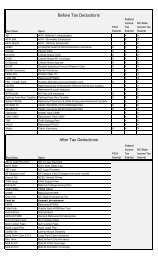
In the screen shot above, the Trait 1 Deletion cell is cleared, meaning this trait will be displayed. An 

asterisk in the Deletion cell a trait means it will not be displayed. 

Click Select All to show all the traits. 

Click Select First to show only the first trait. 

Click Help to display help text for this dialog. 

Note You cannot change the display order of traits. However, you can change the display order of 

chromosomes. 


Selecting chromosomes for graph display 



Select Chrom>Select Chroms… or click when you want to focus the graph on only a few 

chromosomes, rather than all of the chromosomes in the data. Selecting the command displays the 

Select Chromosomes dialog. Use this dialog both to select chromosomes for display and to juggle their 

display order. 

The lower text field shows the chromosomes and the order in which they will be displayed. 

To delete a chromosome from the graph display, click the cell in the Delete row below that 

chromosome. An asterisk in a field means the chromosome will not be displayed; a clear field 

means the chromosome will be displayed. Click the Deletion cell to toggle display on and off. 

In the screen shot above, the Deletion cells for 1, 2, 3, and 6 are cleared, meaning those 

chromosomes will be displayed. When a chromosome is removed from the display, its number 

disappears from the lower text field, also. In the box above, clicking the empty cell under "3" would 

remove chromosome chromo3 from the graph display. 

To reorder chromosomes, click on a number in the Chromosomes row. It swaps places with the 

next displayed cell to its right. Clicking the last displayed cell swaps it with the first displayed cell. 

Example: In the screen shot above, clicking 1 will swap 1 and 2, and the display order will be 2 1 3 

6. Clicking 3 will swap 3 and 6, so the display order would be 1 2 6 3. Clicking 6 will swap 6 and 1, 

so the display order would be 6 2 3 1. 

Click Select All to show all the chromosomes. 

Click Select First to show only the first chromosome. 

Click Help to display help text for this dialog. 


Select Settings>Display Parameters or click from the toolbar to display the Set Graph Display 

Parameters dialog. Use this dialog to refine the display, change font sizes and colors used, and so on.

22 


Show LOD profile as block graph view. Check to show color block for LOD / LR profile instead of line 

curve. Use continuously or block radio button to set the total colors in color block display. 

Ratio between effect window size and LOD window size. Use the spin dials to affect the display 

ratio. You can choose, for example, to make the LOD window the same size as the effect window by 

selecting 1:1. By default, the LOD window is 3 times the effects window size. 

Title. Enter a title for the graph display. Use the X and Y coordinate boxes and the Font size box to 

precisely place the title so it looks as you want. 

Show QTL info. Check to toggle display of QTL information. See Showing QTL information 24 

for more 

information. 

No LOD window. Check to suppress display of the LOD / LR graph window (upper window) and only 

show the effect window. 

No LOD line. Check to suppress display of the LOD / LR line curve in upper window. 




Legend on right. Check to show the legends to the right of the graphs. Uncheck to show the legends 

above the graphs. 

Show trace hairs. By default, WinQTLCart will not show X and Y cross hairs when you select use the 

Trace Position command. Check this box if you do want to see the cross hairs. 

Number of scale lines for X axis. Specify the number of hash marks spread across the cM scale of 

the graph. 

Number of scale lines for Y (LOD) axis. Specify the number of hash marks spread along the LOD 

scale. 

Number of scale lines for Y (effect) axis. Specify the number of hash marks spread along the effect 

scale of the graph. 

Space between two chromosomes. Specify a distance as a percentage of the graph scale to 

separate the chromosomes in the graph. (Put in about 5 or 10 to see the effect.) 

Threshold value for traits. Select a trait from the drop down list and enter a number to set as that 

trait's threshold value. Click the Set all traits with this value button to impose a consistent threshold on 

all displayed traits. 

Trait color and line styles. Select a trait from the drop down list. Press the Color button to select its 

color; select a Line Style from the drop down list to further differentiate it from other traits in the display. 

Maximum LR value in graph. Check and input a value to limit the max LR (not LOD) value into the 

value for the LOD / LR curve line, default value is max LR value in the selected chromosomes and traits. 

Minimum LR value in graph. Check and input a value to set the minimum LR (not LOD) value into the 

value at Y-axis, default value is 8.0. 

Marker label font size. To adjust marker label's font size after selecting showing marker label in LOD / 

LR window. 

Setting a test hypothesis 

Select Setting>Test Hypothesis to play with the results further by trying out different LOD / LR and 

effects (additive, dominant, R2, TR2, S) settings on the displayed results. 

Note: This option is only for crosses with three kinds of genotype such as SF2.

24 


This dialog is fairly self-explanatory. The Hypothesis definitions box describes the conditions for each 

hypothesis, with a=additive and d=dominant. The LR setting box describes pre-set likelihood ratio 

hypotheses. 

Click OK to apply the selected hypotheses options to your display. 


Select Effects>Show QTL Information… or click on the toolbar to display the Show QTL Information 

dialog. From here, you can show QTLs from a simulation parameter file or show summary QTL 

information from the likelihood ratio graph peaks. 

Select the Open QTL information file option and then the Browse… button to select a file that has the 

QTL positions and effects settings you want to use for the display. 

Select the Show one or two LOD interval options, as desired, to show empiric QTL confidence 

intervals—95 percent is one LOD and 99 percent is two LOD. 

Select the Automatically locate QTLs option to specify parameters WinQTLCart will use to find QTLs 

in the results. Use the spin dials to specify the minimum acceptable cM range that defines a QTL peak; 

if the peak's distance is less than this value, then the highest peak will be considered a QTL. The 

minimum acceptable LOD scale as measured by the highest and lowest points of a QTL peak on the 

graph. Both of these requirements must be met for a peak to be considered a QTL. 



Creating simulation data 

WinQTLCart Procedures 

Setting the working directory 



By default, WinQTLCart looks for data files and other working files in its home directory (typically C: 

\NCSU\WinQTLCart) or directory of last opened source data (mcd) file. WinQTLCart saves all files it 

creates to the current working directory. 

But if your data files reside in another directory or on a network drive, you can tell WinQTLCart to look for 

and save its files there. 

1. Select Tools>Set Working Directory to display the Set Working Directory dialog. 

2. To change the directory, click Modify…, navigate to the directory you want, and click OK. The 

new directory appears in the Set Working Directory dialog. 

3. Click Set. 

Importing and exporting 

Importing files 

Unless the files you're working on have already been saved as WinQTLCart mapping source data files 

(files with a .MCD extension) or are already in the .MCD format 39 

, then you need to import them into 

WinQTLCart. WinQTLCart will read in the files, verify the data formatting, and save the files in .MCD 

format automatically. 

WinQTLCart can import files from the following applications: 

Application Formats supported 

MapMaker/QTL .MAP – Map file 

.MPS – Map file 

.RAW – Cross data file 

51 

QTL Cartographer .INP – Map and Cross data files

26 


Microsoft Excel .XLS 

.CSV 

.MAP – Map file 


Note If WinQTLCart displays an error message saying the file format is invalid or can't be recognized, 

then the extension may be wrong or the file's formatting renders it unusable in WinQTLCart. Open 

the file in Notepad and compare it to one of the sample files in the WinQTLCart directory. 

Importing source data files 

1. Select File>Import. The Source Data Import dialog appears. 

2. Select the import option you want. The first extension listed for each option is for the Map file, the 

second extension for the Cross Data file. After clicking Next, the second import dialog appears. 




3. For the MapMaker/QTL and QTL Cartographer options, you need to locate and select the Map 

and Cross Data files by clicking the buttons. For Excel spreadsheets, you only need to specify 

one spreadsheet (WinQTLCart disables the Cross Data button for Excel imports). 

4. By check "Infer map information from cross data file", WinQTLCart will infer map information from 

cross data file by using Emap function. 

5. Enter a file name for the source data file that WinQTLCart will create. You don't need to specify an 

extension—WinQTLCart will take care of that. 

6. Click the Finish button.

28 


7. Emap parameters setting dialog will pop-out if you use Emap function to infer map information. 

Click the button to change random seed for Emap function. 

Linkage map method can take value 10, 11, 12, or 13. 

Segregation test size can be 0.01 to 0.20. 

Linkage test size can be 0.15 to 0.49. 

Now, permutaion function is not active. 

Map function can be Haldane or Kosambi. 

Objuective function can be SAL or SAR. 

8. Set anchor markers by using control group of Anchor marker setting . 

Click to select anchor marker number. 

Click button parameter to open window of Anchor marker parameters set 

Select marker label, chromosome and position on chromosome for each marker (Current 

anchor marker). 

Click button OK to finish parameters set. 


Note: 



If the import was successful, you'll see a dialog saying the files were successfully imported and 

the source data file has been saved. 

If the import didn't work, the reason is likely that the files' formatting does not conform to a 

standard WinQTLCart expects. To troubleshoot 86 this problem, open one of WinQTLCart's 

sample files in Notepad and compare it to the file you specified. (The topic MCD file format 39 

in this manual also describes the file format.) Correct any formatting problems in your specified 

file and try importing again. If you're still unsuccessful, please contact WinQTLCart tech support 

86 . 

More detail help for Emap function, see QTL Cartograhper's manul. 

Notes 

WinQTLCart includes sample source data files for import. Run some tests using these files or open 

them up to see the kind of data formatting WinQTLCart expects to see. 

For Excel worksheets, WinQTLCart expects to see the following worksheet names in the file: 

BasDat, ChrDat, and CroDat. WinQTLCart includes a sample file, NewMcd.xls, that demonstrates 

the formatting it expects to see. (If you want, you can make a copy of NewMcd.xls and modify it for 

your data.) 

For INP format, one cross data file is needed if you use Emap to infer map information. 



Exporting source data and results 

The following table summarizes WinQTLCart's export options: 

1 

Export … …from the… …to… …in these formats… 

Source data Main window QTL Cartographer .INP – Map and cross data files 

Source data Main window QTL Cartographer .MAP – Map file 

30 


30

30 


Source data (minus 

individuals with certain 

OTrait values) 

Source data (one or more 

chromosome(s) with 

reverse marker position) 

Source data (with certain 

selected traits) 

Main window WinQTLCart 30 .MCD (with option to delete 

individuals with a certain OTrait 

value) 

Main window WinQTLCart 30 .MCD (with reverse marker 

position in some chromosomes) 

Main window WinQTLCart 30 .MCD (with some selected traits) 

Source data Main window Microsoft Excel 31 .XLS 

Results Graph window Microsoft Excel 31 .XLS 

Results Graph window Text .TXT (tab-delimited) 

Notes Files are exported to the current working directory 25 . 

Exporting source data to QTL Cartographer 

1. With the source data displayed in the Main window's Data pane, select File>Export. 

2. In the Export Source Data dialog, select one of the following options: 

Select this… …to output these files 

QTL Cartographer INP format .INP files for both the map and cross data 

QTL Cartographer OUT format .MAP for the map file 

.CRO for the dross data file 

3. Edit the Map or Cross filenames, as needed. 

4. Click OK. WinQTLCart exports the files to the current working directory. 

Exporting source data to an MCD file 

Although WinQTLCart saves source data to its own .MCD format, you can use the export dialog to strip 

an .MCD file of individuals with OTrait values. You would do this when you want to analyze the data 

separate from the traits. 

A. MCD file (delete individuals with a certain OTrait value) 

1. With the source data displayed in the Main window's Data pane, select File>Export 

2. In the Export Source Data dialog, select MCD file (delete individuals with a certain OTrait value). 

3. Edit the source file name, as needed. The file will be saved to the current working directory 25 . 

4. From the OTrait Value pull-down menu, select the trait to be stripped from the MCD file. 

5. Click OK. WinQTLCart exports the file to the current working directory 25 . 

B. MCD file (reverse one or several chromosomes) 


2. In the Export Source Data dialog, select MCD file (reverse one or several chromosomes). 


4. From the Chrom. Number Edit Box, type in chromosome numbers separated by comma. 

5. Click OK. WinQTLCart exports the file to the current working directory 25 

. 


C. MCD file (only selected traits are included) 




2. In the Export Source Data dialog, select MCD file (only selected traits are included). 


4. From the Trait Number Edit Box, type in trait numbers separated by comma or hyphen. 

5. Click OK. WinQTLCart exports the file to the current working directory 25 . 

Exporting results from the Graph window 

The Graph window doesn't export results, per se (there's no Export menu), but you can save the results 

in these formats: 

WinQTLCart mapping result file (.QRT). 

Excel file (.XLS), LR/LOD values to a worksheet labeled "LR", QTL information to a worksheet 

labeled "QTLs", and points obtained through graph trace function to a worksheet labeled "Points". 

Text file (.TXT), in a tab-delimited format. 

Simply select the appropriate command from the Graph window's File menu, specify the directory and 

filename in the Save As dialog, and click OK. WinQTLCart will display a confirmation dialog that the file 

has been created. 

Working with source data files 

WinQTLCart's source data files have a .MCD extension. A .MCD file is a text file that adheres to a 

specific format 39 that includes all the information WinQTLCart needs for QTL mapping analysis. 

When you open a source data file 32 , WinQTLCart verifies the file's formatting and displays its basic 

information in the Main window's Form pane. 

Note Although you can open other text and result files in WinQTLCart, only .MCD file information is 

displayed in the Form pane. WinQTLCart will continue showing the last .MCD file you viewed in 

the Form pane, even if you open or switch to text or result files. 

The Summary Information box tells you the basics on the selected source data file. From here, you can 

go ahead and select an analysis method, if you wish. 

However, the form's buttons and pull-down lists let you look at the source data file in more detail and 

also perform the following actions: 

View information of markers, traits and other traits (also called categorical traits) in a formatted 

way. 

Add/edit/delete marker genotype data 32 

for each chromosome in the file, including adding or

32 


deleting individuals 

Add/edit/delete trait values 33 and other traits 

Edit map 34 and cross 35 information 

Add new experimental data (individuals) 

Try out different data configurations, such as retaining certain individuals' chromosomes 

You may find that you need to add, edit, or delete data due to import errors. Some errors can be caused 

by mistaking cross data for map data, and vice versa. 

WinQTLCart's tools for editing marker, trait, and other information offer a safer and more organized 

approach than if you were to do the same thing by hand in a text editor. If you need to alter the source 

data's information in any way, it is highly recommended you use WinQTLCart. 

Opening source data files 

There are several ways to open a prepared source data file from the Main window. 

Select File>Open 

Click the Open button on the toolbar 

Use the keyboard command Ctrl+O 

Double-click or right-click on the Source Files node in the Tree pane 10 

Any of these methods opens the standard Windows Open dialog box. The dialog defaults to the current 

working directory 25 

. If you open an .MCD file from a different directory, WinQTLCart will save the 

mapping result files to that location. 

Also you can double click a .MCD file in Windows File Explorer to open the source data file 

automatically. 

Working with a source file's marker genotype data 

At the Source data view and modify pane on the Main window, select the chromosome you want to work 

with from the pull-down list and click Markers button to open the Marker Information dialog. 

At the Marker Information dialog, Marker Labels are the column headings, Individuals are the rows. You 

can enlarge the dialog by dragging its border toward or away from the center of the screen. (The pointer 

is a two-headed arrow when it is in the correct position.) 


Changing a cell's contents 



For modifying a cell's value, click in the cell and type in a new value. (Or, click in a cell and enter the 

value in the Edit selected cell value field.) 

You can change as many cells as you like. Click Update Cell to save your changes as you go. you can 

click OK to save all changes and close the dialog. 

Click Cancel to close the dialog without saving any of your changes (including any changes saved with 

the Update Cell button). 

Working with a source file's traits values 

Traits: At the Trait values pane on the Main window, click the Trait View button to open the Trait 

Information dialog. 

Other Traits: If the source data file contains other traits, then click the OTrait View button to open the 

Other Trait Information Dialog. 

For more information on working with this dialog, and on modifying values, see the following topics: 

Working with a source file's marker genotype data 32

34 


Working with a source file's basic information 

At the Source data manipulations pane on the Main window, click the Basic Info button to open the 

Manipulation of Basic Information dialog. 

Symbol for missing trait value. Enter a symbol to use for missing traits value, based on your trait 

data. 

Marker translation table. Edit or add symbols you want to use for these genotype markers; you can 

enter any alphanumeric character(s) as a symbol. These translations apply to the experimental design 

you selected at the left of the dialog. 

Note WinQTLCart assumes that the A allele is diagnostic for the High (parental 1) line and the a 

allele is diagnostic for the Low (parental 2) line. A minus sign (-) means the allele is unknown. 

WinQTLCart uses the numbers (2, 1, 0, 12, 10, -1) to determine how to encode the output of 

the genotypes. The alphanumeric tokens you enter here indicate how you have coded the 

markers in the source data. 

Cross Information 

Select the experimental design option based on your data. You can select only one option. 

B1. Backcross, with 1=parental line to which the F1 line was crossed. 


Ri0. Recombinant inbred line, derived by doubled haploid lines. 

Ri1. Recombinant inbred line, derived by selfing. 

Ri2. Recombinant inbred line, derived by sib mating. 

SF. Selfed intercross line. Enter an integer indicating the generation. Limit of 2. 

RF. Randomly mated intercross line. Enter an integer indicating the generation. 




T(B1)SF. Test cross, with genotyping done on an intercross (SF) and phenotyping on a cross (B1) 

derived from that intercross. Enter an integer indicating the generation. 

T(B1)RF. Test cross, with genotyping done on an intercross (RF) and phenotyping on a cross (B1) 


T(B2)SF. Test cross, with genotyping done on an intercross (SF) and phenotyping on a cross (B2) 


T(B2)RF. Test cross, with genotyping done on an intercross (RF) and phenotyping on a cross (B2) 


Map Function 

A map function is a mathematical relationship between recombination probabilities and map distances. 

Select the function you want, based on the interference to be assumed. 

Haldane. The default option. Assumes no crossover interference. 

Kosambi. Assumes some interference. 

Fixed. The Morgan mapping function. Assumes complete interference. 

Note These mapping functions, among others, are discussed at length in Ben Lui's book, 

Statistical Genomics: Linkage, Mapping and QTL Analysis (1998). 

Distance type 

Position. Indicates that the numbers indicate positions from the left telomere of the current 

chromosome. This means the numbers should be in increasing order. 

Interval. Indicates that the numbers are for the interval distance after a marker. This means that 

the last number, and the last number only, should be zero. 

Distance units 

centiMorgan (cM). Very small. 100 centiMorgans=1 Morgan. 

Morgan. The distance over which, on average, one crossover occurs per meiosis. 

Recombination. Percentage of crossover events that occur between two markers. 

Related Topics 

MCD file format 

39 

Working with source file's individual information 

At the Source data manipulations pane on the Main window, click the Individual button to open the Add 

or Delete Individuals dialog.

36 


Append and Delete. Click Append radio button to add individual(s) into active source data and click 

Delete radio button to delete one or more individual from active source data. 

1. Append individual(s) 

WinQTLCart can read the individual information through a properly formatted text file (data separated by 

spaces, not commas) and click Filename button to indicate the filename. (Use the Notepad button to 

call up an empty text file if you need to do impromptu editing.) To check From Clipboard button if the 

individual information is already in Windows clipboard. Please check the Data include individual label(s) 

button if the individual data include individual label. Click OK button to append the individual(s) after set 

the correct Total (individual) number. 

There are two ways to read data. 

If your data is... Then click... Comments 

In a text file Filename… to display the 

Open dialog box. 

On the Windows clipboard Data from clipboard check 

it to transfer the data to the 

edit window. 

2. Delete individual(s) 

In the Open dialog, select the 

text file that has the values you 

want to add and click OK. 

You should select and copy 

the data in other text editor 

such as Windows notepad. 

In the Individual Number text edit box, enter the individual(s) you want to delete, separated by commas 

or hyphen. Click OK button to finish. 


Working with source file's chromosome information 



At the Source data manipulations pane on the Main window, click the Chromosome button to open the 

Chromosome and Markers Manipulation dialog. 

Add and Delete. Click Add radio button to add a chromosome or a marker into active source data and 

click Delete radio button to delete current chromosome or marker(s) in current chromosome from active 

source data. 

Select chromosome. Select one chromosome from the pull-down menu as the current chromosome. 

1. Insert one marker in current chromosome 

WinQTLCart can read the marker information through a properly formatted text file and click Filename 

button to indicate the filename. To check From Clipboard button if the marker information is already in 

Windows clipboard. 

2. Insert one chromosome 

WinQTLCart can read the chromosome information through a properly formatted text file and click 

Filename button to indicate the filename. To check From Clipboard button if the chromosome information 

is already in Windows clipboard.

38 


3. Delete current chromosome 

Click Delete current chromosome radio button and click OK button. 

4. Delete marker(s) in current chromosome 

Click Delete markers radio button and in the Marker Number text edit box, enter the marker(s) you want 

to delete, separated by commas or hyphen. 

Working with source file's trait information 

At the Source data manipulations pane on the Main window, click the Trait button to open the Add or 

Delete Traits dialog. 

Add and Append. Click Append radio button to append trait(s) into active source data and click Delete 

radio button to delete trait(s) from active source data. 

1. Append trait(s) 

WinQTLCart can read the trait information through a properly formatted text file and click Filename 

button to indicate the filename. To check From Clipboard button if the trait information is already in 

Windows clipboard. Please check the Data include trait label(s) button if the trait data include trait label. 

Click OK button to append the trait(s) after set the correct Total (trait) number. 

2. Delete trait(s) 

In the Trait Number text edit box, enter the Trait(s) you want to delete, separated by commas or 

hyphen. 


Working with source file's other trait information 



At the Source data manipulations pane on the Main window, click the OTrait button to open the Add or 

Delete Other Traits dialog. 

Add and Append. Click Append radio button to append other trait(s) into active source data and click 

Delete radio button to delete other trait(s) from active source data. 

1. Append other trait(s) 

WinQTLCart can read the other trait information through a properly formatted text file and click Filename 

button to indicate the filename. To check From Clipboard button if the other trait information is already in 

Windows clipboard. Please check the Data include otrait label(s) button if the other trait data include 

label. Click OK button to append the other trait(s) after set the correct Total (other trait) number. 

2. Delete other trait(s) 

In the OTrait Number text edit box, enter the Other Trait(s) you want to delete, separated by commas or 

hyphen. 

MCD file format 

WinQTLCart .MCD source data files use tokens to indicate the meaning of data. This topic describes 

valid tokens used in .MCD source data files. 

The line numbers in this topic refer to the sample .MCD file, "NewMcd.mcd," which is included as part of 

the WinQTLCart distribution. 

Token #FileID (line 1)

40 


File's ID number; usually a 10-digit number. 

Token /* and */ (Lines 2 – 5) 

Insert multiple-line comments between these tokens. 

Token #bychromosome (Line 6) 

Indicates start of chromosome information. 

Token // (Lines 6 – 10) 

Insert one-line comments after the double-slash. 

Token –type (Line 7) 

Indicates how marker positions are numbered along the chromosome. It takes one parameter that can 

be either "position" or "interval". 

Position indicates that the numbers are positions from the left telomere of the current chromosome. 

So numbers should be in increasing order. 

Interval indicates that the numbers are the interval distance after a marker. So the last number 

and only the last number in the series should be zero. 

-type 

position 0.0 9.3 17.2 29.9 38.7 52.8 57.8 72.4 76.6 93.2 97.0 115.5 

116.5 

interval 9.3 7.9 12.7 8.8 14.1 5.0 14.6 4.2 16.6 3.8 18.5 1.0 0.0 

Token –function (Line 8) 

Indicates which map function is used to transfer recombination frequency (r) between markers to 

distance in Morgan (M). The parameter can be an integer from 1 – 8. Haldane and Kosambi are the two 

most useful map functions. 

Code Reference Note 

1 Haldane (1919) Default 

2 Kosambi (1944) 

3 Morgan (1994) "Fixed" 

4 Carter and Falconer (1951) 

5 Rao et al. (1979) 0 £ p £ 1 

6 Sturt (1976) L 

7 Felsenstein (1979) -¥ < K < ¥, K ¹ 2 

8 Karlin (1984) Binomial, N > 0 

The following Haldane and Kosambi formula can be used to convert marker distance from r to M or vice 

versa. 

------------------------------ 

Haldane: dM = -0.5ln(1-2r) r = 0.5(1-exp(-2dM) 

Kosambi: dM = 0.25ln((1+2r)/(1-2r)) r = (1-exp(-4dM))/(2(1+exp(-4dM))) 

------------------------------ 

Token –Units (Line 9) 

Indicates unit of marker positions. There are three choices: 

cM (centiMorgan) 

M (Morgan) 




r (Recombination frequency) - If you choose this parameter, then token -function should be 3 

(Morgan) 

Token –chromosome (Line 10) 

Indicates total number of chromosomes for source data. 

Token –maximum (Line 11) 

Indicates the maximum number of markers for a chromosome for all of the source data. 

Token –named (Line 12) 

Either yes or no. 

Yes means markers have names 

No means markers will not have names. 

Token –start and –end (Line 13 and Line 55) 

Use these tokens to start and end the marker position data of all chromosomes. 

Token –Chromosome (Line 14, 28, and 41) 

Indicates chromosome name. The marker position data for this chromosome will start with the next line. 

Token #bycross (Line 56) 

Indicates that cross information is to begin. 

Token –SampleSize (Line 57) 

Indicates sample size or individual number. 

Token –Cross (Line 58) 

Indicates codes for crosstype mating design (see the following table). 

Code Design Examples 

Bi Backcross to Pi B1, B2 

Bij Backcross j times to Pi B13, B25 

SFi Selfed generation i intercross SF2, SF6 

RFi Randomly mated generation i intercross RF2, RF3 

RI0 Doubled haploid RI0 

RI1 Recombinant inbred via selfing RI1 

RI2 Recombinant inbred via sib mating RI2 

T(Bi)SFj Testcross of SFi to Pj T(B1)SF3 

T(SFi+j)SFi Testcross of SFi for j generations T(SF4)SF3 

T(Bj)RFi Testcross of RFi to Pj T(B1)RF3 

T(D3)SFi Design III T(D3)SF5 

Token –traits (Line 59) 

Indicates trait number of source data. 

Token –otraits (Line 60) 

Indicates other trait number of source data. Other trait (also called a categorical trait) is the trait with 

qualitative or categorical values, such as sex; color, and so on. Other traits can be used as factors that 

can be "regressed out" in regression analysis. This means a regression of the quantitative trait of 

interest on the categorical trait will have been performed and the residuals used as the phenotypes in the 

analysis.

42 


Token –missingtrait (Line 61) 

Indicates the symbol for missing trait value. 

Token –case (Line 62) 

Either yes or no. 

Yes means all comparisons are case dependent. 

No means all names of individuals, markers and traits are converted to lower case to make 

comparisons. 

Token –TranslationTable (Line 62) 

The token with the table (next 6 lines of data) will define how marker genotype data are translated. There 

are six rows and three columns (18 positions) in the table. Here is the default translation table: 

-TranslationTable 

AA 2 2 

Aa 1 1 

aa 0 0 

A- 12 12 

a- 10 10 

-- -1 -1 

The first column is the genotype. The program assumes that the A allele is diagnostic for the High 

(parental 1) line and the a allele is diagnostic for the Low (parental 2) line. A minus sign (-) means 

the allele is unknown (missing). Dominant as well as co-dominant markers can be encoded. 

The middle column is how the output of these genotypes will be encoded. 

The third column is how you will code the marker genotype data in this source data file. Just about 

any set of tokens can be used for the third column (corresponding to your dataset), but DO NOT 

change the first two columns. 

The above TranslationTable maps 2 to 2, 1 to 1, 0 to 0, etc. Just about any set of tokens 

can be used for the third column, but DO NOT change the first two columns. If you encoded 

your P1 homozygotes as BB, heterozygotes as Bb, etc, your translation table might appear as: 

-TranslationTable 

AA 2 BB 

Aa 1 Bb 

aa 0 bb 

A- 12 B 

a- 10 b- 

-- -1 -- 

Anything in the data file that is not recognized (doesn't match something in 

column 3) will become unknown (-1) in the output. 

Important: You need all 18 tokens following the -TranslationTable token and the 

first two columns can't be altered. You should only alter the last column. 

Token –start markers and –stop markers (Line 70 and Line 109) 

Use these tokens to start and end the marker genotype data of all chromosomes. Please keep the 

same chromosome and marker order as the data between token –start and token -end above. 

You can organize the data by marker or individual: 

Order by marker: For each marker, you provide the genotype data for all individuals. The order of the 




individuals must be the same for each marker. 

Order by individuals: For each individual, you provide the genotype data for all markers (all 

chromosomes). The order of chromosomes and markers has to be the same. 

-start individuals markers 

Ind1 2 2 1 1 2 2 2 2 2 

Ind2 2 2 2 1 2 1 2 2 1 

Ind3 2 2 2 2 2 1 2 1 1 

Ind4 2 1 2 2 2 2 1 1 1 

Ind5 2 1 2 2 2 2 1 1 1 

-stop individuals markers 

Note that the tokens are different and the first column is the individual's label. 

Token –start traits and –stop traits (Line 110 and Line 114) 

Use these tokens to start and end the trait values. The data should be organized by the trait's order for 

the trait value. That is, for each trait, you give the trait value of all individuals. If organized by the 

individual, then for each individual, you provide the trait value of all traits. 

-start individuals traits 2 Trait_1 Trait_2 named 

Ind1 5.0 15.0 

Ind2 5.3 15.3 

Ind3 6.2 16.2 

Ind4 4.1 24.1 

Ind5 5.5 25.5 

-stop individuals traits 

Note that the tokens are different and there are trait number and trait labels after the token -start 

individuals traits. The label "named" means data has trait names. 

Token –start otraits and –stop otraits (Line 115 and Line 118) 

Use these tokens to start and end the other trait values. The data must be organized by the other trait's 

order; that is, for each other trait, you give the other trait value of all individuals. If you order by 

individuals, then for each individual, you give the other trait value of all other traits. 

Example: 

-start individuals otraits 2 sex brood named 

Ind1 M 1 

Ind2 F 1 

Ind3 M 0 

Ind4 M 1 

Ind5 M 1 

-stop individuals otraits 

Please notice that the tokens are different and there are other trait numbers and other trait labels after 

the token -start individuals otraits. Label "named" means data has other trait names. 

Token –quit and –end (Line 119 and Line 120) 

Indicate the end of the source data file. 

Token -population 

Indicate the population number and the rest of .MCD filename. 

Please notice that you should build one .MCD file for each population. 

Example:

44 


-population 4 env2-jun3.mcd env3-jun3.mcd env4-jun3.mcd 

There are totally 4 populations and the 4 .MCD files include current file, and file "env2-jun3.mcd", file 

"env3-jun3.mcd" and file "env4-jun3.mcd". All .MCD files should be in same directory. 

Token -xchromosome 

Indicate the X chromosome number and cross type that will not be the same as rest of chromosomes. 

Creating a new source data file from raw data 

WinQTLCart can help you convert your raw source data (including map and cross information) into 

formatted MCD files. WinQTLCart can run analysis methods only on MCD files. 

The goal of this process is to create a file that looks like the MCD data file (described in the MCD data 

file format 39 

topic). Although WinQTLCart can't automate this process for you, it does provide you with 

tools to make a clean transition from raw source data to rigorously formatted data file. 

The easiest way to work with this function is to have individual, properly formatted text files for each data 

type (marker genotype, individuals, etc.). Individual files are quicker to select and import. Otherwise, you 

do have to do a lot of copy and paste. 

Here's a checklist of files you should have on hand, along with sample files in the WinQTLCart2.5\Add- 

New directory you can use to create your own files. 

Chromosome labels and number. See 201-chlab-mknum.txt 

Marker labels. See 301-mklab.txt that shows one file for all chromosomes. 

Marker positions. See 302-mkpos.txt that shows one file for all chromosomes. 

Marker genotypes. One file for all chromosomes and there are 4 different cases: 

Case 1: Individual order with individual label, See 521-mkgen-ind-lab.txt 

Case 2: Individual order without individual label, See 521-mkgen-ind-nolab.txt 

Case 3: Marker order with marker label, See 541-mkgen-mk-lab.txt 

Case 4: Marker order without marker label, See 541-mkgen-mk-nolab.txt 

Trait values and labels. One file for all traits: 

Case 1: Individual order with trait label, See 522-tt-ind-lab.txt 

Case 2: Individual order without trait label, See 522-tt-ind-nolab.txt 

Case 3: Trait order with trait label, See 542-tt-tt-lab.txt 

Case 4: Trait order without trait label, See 542-tt-tt-nolab.txt 

Other trait values and labels. One file for all other traits: 

Case 1: Individual order with other trait label, See 523-ot-ind-lab.txt 

Case 2: Individual order without other trait label, See 523-ot-ind-nolab.txt 

Case 3: other trait order with other trait label, See 543-ot-ot-lab.txt 

Case 4: other trait order without other trait label, See 543-ot-ot-nolab.txt 

An alternative to use separate files is to create a single file holding marker genotype, trait, and other trait 

information. But the data must be in individual order: 

Case 1: has individual label, See 511-mkttot-lab.txt 

Case 2: has not individual label See 511-mkttot-nolab.txt 

1. Select File>New to open the Create New Source File – Step 1 of 6 dialog box. 


Fill in the dialog based on your source data. 



Basic information group box 

Chromosome number. Enter the number of chromosomes in the source data. 

Trait number. Enter the number of traits in the source data. 

Other trait number. Enter the number of other traits in the source data. ("Other traits" are 

also known as categorical traits.) 

Individual number. Enter the number of individuals in the source data. 

Symbol for missing trait value. Enter a symbol to use for missing traits, based on your trait 

data. 

Crossing type. Select the correct cross type for your data: 



Ri0. Recombinant inbred line, derived by doubled haploid lines. 

Ri1. Recombinant inbred line, derived by selfing. 

Ri2. Recombinant inbred line, derived by sib mating. 

SF. Selfed intercross line. Enter an integer indicating the generation. Limit of 2. 

RF. Randomly mated intercross line. Enter an integer indicating the generation. 

T(B1)SF. Test cross, with genotyping done on an intercross (SF) and phenotyping on a 

cross (B1) derived from that intercross. Enter an integer indicating the generation. 

T(B1)RF. Test cross, with genotyping done on an intercross (RF) and phenotyping on a 


T(B2)SF. Test cross, with genotyping done on an intercross (SF) and phenotyping on a 


T(B2)RF. Test cross, with genotyping done on an intercross (RF) and phenotyping on a 

cross (B2) derived from that intercross. Enter an integer indicating the generation.

46 


Marker genotype table. Edit or add tokens you want to use for these genotype markers; you 

can enter any alphanumeric character(s) as a token. These translations apply to the Crossing 

type you selected from the drop down. You must ensure that the chosen symbols in this 

translation table match those in your marker genotype data file. 

Note WinQTLCart assumes that the A allele is diagnostic for the High (parental 1) line and 

the a allele is diagnostic for the Low (parental 2) line. A minus sign (-) means the allele 

is unknown. WinQTLCart uses the numbers (2, 1, 0, 12, 10, -1) to determine how to 

encode the output of the genotypes. The alphanumeric tokens you enter here indicate 

how you have coded the markers in your source data. 

Source data file stem name. Enter a name for your source data file. As WinQTLCart creates 

new source data files, WinQTLCart will append extensions to this stem. 

2. Click Next button to accept the values. The Create New Source File – Step 2 of 6 appears. 

Fill in the dialog based on your source data. 

Map function. A map function is a mathematical relationship between recombination probabilities 

and map distances. Select the function you want, based on the interference to be assumed. 

Haldane. The default option. Assumes no crossover interference. 

Kosambi. Assumes some interference. 

Fixed. The Morgan mapping function. Assumes complete interference. 

Position type 






Interval. Indicates that the numbers are for the interval distance after a marker. This means 

that the last number, and the last number only, should be zero. 

Position units 

centiMorgans (cM). Very small. 100 centiMorgans=1 Morgan. 

Morgan. The distance over which, on average, one crossover occurs per meiosis. 

Recombination. Percentage of crossover events that occur between two markers. 

Data-window. All the numbers you see here are place holders, waiting for you to input the real 

data. 

Edit window. Data from your raw data file (or in Windows clipboard) is copied to this window 

first. You can edit data in this window. 

Browse Displays Windows Open dialog so you can select the data file. Selecting the file copies 

its contents to the Edit window. 

Clipboard. Paste contents of Windows clipboard to Edit window. 

Send Data. Check Include label if necessary, then click Send Data to update the data-window. 

Notepad. Open a blank Notepad file, for use as a holding area for data, provide an editing 

scratchpad, and so on. 

3. Click Next button to accept the values. The Create New Source File – Step 3 of 6 appears.

48 


Click radio button Labels to input and send marker label information and click radio button Positions to 

input and send marker positions information. Other operation is similar to above step 2. 



First to specify raw data file's number by click one of the radio button. 

1. All data in one file 



Use one file that includes marker genotype, trait, and other trait information. Select Data format 1 

in Select data format of one raw file situation group box if the data include individual label. Otherwise 

select Data format 2. All data must arrange according to individual order. 

2. Data in three files 

Use three files for marker genotype data, trait data, and other trait data. For each file, you can 

choose arrange according to individual or according to marker (trait, or other trait) in Select data 

format of three raw files situation group box. To check corresponding box if there are labels in file. 

5. Click Next button to accept the values. The Create New Source File – Step 5 of 6 appears.

50 


Please notice that the buttons in this dialog is depend on the selections of previous dialog. 

For marker genotype information, use Browse button to indicate the filename and Send Data button to 

update the Data-Window. It is same for the trait value also. The Browse and Send Data button will be 

disabled if there is no other trait, Otherwise, you can do the same as trait value. 

Only one set of Browse and Send data button will be enabled if you choose one data file format in the 

previous dialog. 

Note: The Data file's format should be comparable with the setting of previous dialog. For example, if 

there is no individual label in the genotype data file and you check the include individual labels button 

in previous dialog. Then a warning message box will pop-out when you click the Send Data button in 

Marker genotype filename group. 





This is the data summary dialog. The up window is map information and lower window is cross 

information. Click Back button to do the modification if the information is not right. After you check all 

the necessary data, click Finish button WinQTLCart will: 

Verify the data and display error messages if the data file is incomplete or formatted 

incorrectly. 

Create the .MCD file using the filename stem you entered at the first Create New Source File 

dialog. 

Show a create .MCD file successful dialog, click OK button to the dialog and display the 

Main window, with the MCD file you just created loaded into the Source Data form. 

Where to go from here 

Select an analysis method 

Creating simulation data 

2 

To use WinQTLCart's results graphing abilities, you need data for it to work on. If you haven't collected 

any data, though, you can still simulate a dataset that WinQTLCart can work with. 

To create a data simulation file, select File>Simulation. This displays the Create Simulation Data series 

of dialogs.

52 


Fill in the blanks for yourself, or accept the defaults. 

Random seed. Click the button to generate a new random seed. 

Replications. Produce a file with many replications of simulation data with the same parameter setting. 

The filename look like ***SimuRep-1.dat and the ***.mcd is the simulation .MCD file. 

Sample size. Individual number. 

Map function. Haldane (assumes no crossover interference) or Kosambi (assumes some crossover 

interference). 

Total Trait. Indicate how many traits in the simulation data. 

Current Trait. You can change the current trait and set parameter of Trait mean. 

Cross Information. Select an experimental design option. You can select only one option to modify at a 

time. (At this time, only the three options below are available for selection.) 



SF2. Selfed intercross line, generation 2. 

Translation table. Edit or add tokens you want to use for these genotype markers; you can enter any 

alphanumeric character(s) as a token. 

Note WinQTLCart assumes that the A allele is diagnostic for the High (parental 1) line and the a 

allele is diagnostic for the Low (parental 2) line. A minus sign (-) means the allele is unknown. 




WinQTLCart uses the numbers (2, 1, 0, 12, 10, -1) to determine how to encode the output of 

the genotypes. The alphanumeric tokens you enter here indicate how you have coded the 

markers in the source data. See the topic MCD file format 39 

for more information. 

Chromosome and marker information 

Total chromosome number. The total number of chromosomes. Click the spin dial to the 

right of this field to select more or fewer. 

Current chromosome. Shows the active chromosome you're working on. Click the spin dial to 

the right of this field to select a new chromosome. You'll see the new chromosome's 

information in the Distance and Label boxes to the right. 

Markers for chromosome. Total number of markers for this chromosome. 

Average space between markers (cM). Produces marker positions randomly. 

Variations of the marker positions (%). How many deviations are allowed, on average 

Check Read marker positions from a text file and click Browse to select a text file 

containing that information. Also, select a marker distance type. 



Interval. Indicates that the numbers are for the interval distance after a marker. This means 

that the last number, and the last number only, should be zero. 

From QSI file. To produce the simulation data by loading a QSI file alone. In Step 3, you can save all 

simulation parameters into a QSI file. 

Filename. The file name of the MCD file that will be created. 

Directory. The directory that the simulated MCD file will be created.

54 


Next Trait. Click this button to reach each trait and you can set following parameters. 

QTL numbers. Set the number of QTLs to appear in the file. 

Heritability. Requires a value in the range 0.0 to 1.0. Default is 0.8. 

Vd/Va. Dominant variance/Additive variance 

Vi/Va. Epistatic variance/Additive variance 

For the Additive, Dominant, and Epistatic effects you want to see in the simulation, you can select 

the following: 

Effects direction 

Same—All values are positive 

Both—Values are positive and negative 

Sign's Ratio—Ratio of negative:positive. 

Effects distribution 

Equal—All effects have the same value 

Normal—Values derive from normal distribution 

Gamma—Values derive from gamma distribution 

Parameter—Value for gamma distribution 

Note For more information on effects distribution and the additive, dominant, and epistatic effects, 

please refer to the QTL Cartographer's manual. 

After inputting the parameters in the previous two dialogs, the final dialog presents the data simulation 

model you have built. Click in any cell to see that cell's values represented in the fields below. 

Next Trait (or First Trait). Click this button to reach each trait. 

Use the fields to edit a cell's contents. Click the Update button to write the change to the model. 

Click Save to save your model to a .QSI (QTL Simulation Information) file. The current working 




directory is selected as the default. (Click the X in the dialog's upper right corner to close without 

saving.) 

Click Load to load a .QSI file to this window. The file's values replace the values you see in the 

current window. 

Click Adjustment to adjust values for the entire genome. 

Click OK to produce the simulation data file. You can then use that file for analysis. 



Single-marker analysis 

24 

When to use 

For quick scanning of the entire genome (all chromosomes) to find best possible QTLs and identify 

missing (or incorrectly formatted) data. Use single-marker analysis first to ensure your data file is clean; 

then move on more sophisticated analysis methods, such as Interval Mapping 58 and Composite Interval 

Mapping 60 

. 

How it works 

Single-marker analysis is based on the idea that if there is an association between a marker genotype 

and trait value, it is likely that a QTL is close to that marker locus. 

Comments 

Single-marker analysis can be somewhat useful for a quick look at data, but it has been superceded by 

Interval Mapping and Composite Interval Mapping. IM and CIM are more thorough and accurate indicators 

of QTL. The prime value of WinQTLCart's single-marker analysis is its identification of missing data that 

could affect later analysis. 

Running a single-marker analysis 

1. Open a mapping source data file (an .MCD file) into the WinQTLCart main window. 

2. Select Method>Single-Marker Analysis. WinQTLCart analyzes the data and displays the singlemarker 

analysis controls in the form pane. The information pane on the right includes the analysis 

results. 

3. Select a trait for display from the Trait Selection pull-down list. All the traits present in the file will 

be on the list. 

4. For each trait, the information pane on the right displays WinQTLCart's statistical summary of the

56 


file. (You can view this summary in a larger window by clicking the Result button in the Statistical 

Summary group box, just to the left of the information pane.) 

5. In the Single Marker Analysis group box, click Result to view the analysis result for the selected 

trait. You can change the font used by the display window to make the results easier to read. 

Click the Save… button in this group to save the marker analysis results to a text file. 

6. In the Statistical Summary group box, click Result to view the summary in a larger display 

window. Click the Save… button to save the statistical results to a text file. 

The statistical summary includes: 

Basic summary of the data 

A histogram for the quantitative trait 

WinQTLCart's summary of missing individuals that should be present, as indicated by the 

data. If markers show 0% data, there was likely an import problem. 

Summary of marker segregation 

Combines LR map QTL and Q stats 

7. Click the Graphic File… button to save the results to a QTL mapping result file (*.QRT). You can 

open this .QRT file later to view the results as a graph. 

8. Click Close to end the single-marker analysis session and return to the Form View of Source 

Data. 

Qstats show some important results: 

Tells you that the data were imported correctly. If a marker has 0% data, that indicates a problem 

(likely an import problem). For example, the original marker may be *Marker_1, but QTL sees 

that as *Marker-1, and the values won't match. 

Tests for segregation distortion 

Setting threshold levels (IM & CIM) 

Both Interval Mapping 58 and Composite Interval Mapping 60 use threshold values to determine QTLs. If 

you don't know the threshold value for a trait, you can have WinQTLCart find them out and use them as 

inputs for the QTL search. 

The threshold levels control the rate of Type 1 errors (false positives). A lower threshold value means 

more false positives; but a higher value means you may miss more QTLs. 

When you look at a result graph 17 

, the horizontal line you see running across the graph is the 

threshold level. When the graph peaks over the threshold level, that is good evidence for a QTL. So, 

setting the threshold level in this form controls how high or low that line will sit on the graph. Too high 

and you'll see no QTLs; too low and you'll see too many. (The threshold value can be changed later in 

the Graph window.) 

Getting a very accurate threshold level may take a long time. Recommendations are included in the 

threshold procedures. 

1. Follow the instructions for the form you're working with (either IM or CIM). Be sure to select a trait 

or all traits for which you want to set a threshold level. 

2. The Threshold group box on the right of the form controls inputting or obtaining mapping threshold 




values for each trait. Select a different trait number to see the threshold value of that trait. 

3. Select whether you want to set the threshold levels manually or have WinQTLCart determine the 

threshold via permutations. 

If you... Do this... Comments 

Know the threshold values you 

want to use 

Don't know the threshold values 

you want to use 

Setting threshold levels manually 

Input them into the Manual Input 

57 box 

Select By Permutations 57 

to have 

WinQTLCart calculate them. 

This analysis occurs before you start the QTL analysis. 

Permutations take a long time to 

run. If 1 permutation runs for 10 

seconds, than 1000 permutations 

will take 2-3 hours. 

Use this procedure to set the threshold for each trait manually. This is useful if you know the value for 

each trait. Alternatively, select All Traits and apply this threshold setting to all the traits. 

1. From the Trait Selection pull-down, select a trait to find the threshold value for that trait. (The All 

Traits selection is available for permutations only.) 

2. Click the By Manual Input option. 

3. Input a threshold value into the box. 

4. Optional: Click Set as Default if you want to assign the threshold value you entered to all traits. 

Setting threshold levels via permutations 

This analysis occurs before you start the QTL analysis. 

Setting values via permutations allows WinQTLCart to empirically estimate the genome-wide significance 

threshold. Use this procedure if you don't know the value and you want WinQTLCart to find the optimal 

threshold. 

Threshold values will be filled in automatically for every trait according to significance level. 

Following threshold analysis, WinQTLCart will display the results in the Data pane and save them in a 

text file. The text file's name is displayed in the form after the analysis completes. 

1. From the Trait Selection pull-down, do one of the following: 

Select one trait to find the threshold value for that trait. 

Select All Traits to find threshold values for all traits. 

2. Click the By Permutations option. 

3. Enter a value for Permutation Times to set the permutation repeating times. 

Note If you want a quick run, use the default value of 300. But if you're going to publish, use 

the 1000 value; this will take several hours to run but will yield very precise results. We 

recommend starting this analysis before you leave for the day and letting it run 

overnight. 

4. Enter a value for Significance Level. 

5. Click OK to begin threshold analysis.

58 


Note You cannot update the All Traits checkbox. WinQTLCart checks or clears this box based on 

whether you select one or all traits from the drop down list. 

After you click OK, WinQTLCart displays a countdown showing its progress through the file. When the 

threshold analysis is complete, WinQTLCart will display the results in the Data pane and display the 

results file's name. (WinQTLCart saves the file to the current working directory 25 .) 

After setting the threshold value, move on to finish the IM 58 or CIM 60 analysis procedure. 

Interval Mapping 

What it is 

Interval mapping (IM) is an extension of single-marker analysis 55 . In single-marker analysis, only one 

marker is used in QTL mapping but effects are underestimated and the QTL position cannot be 

determined. Interval mapping provides a systematic way to scan the whole genome for evidence of QTL. 

IM uses two observable flanking markers to construct an interval within which to search for QTL. A map 

function (either Haldane or Kosambi) is used to translate from recombination frequency to distance or 

vice visa. Then, a LOD score is calculated at each increment (walking step) in the interval. Finally, the 

LOD score profile is calculated for the whole genome. When a peak has exceeded the threshold value, 

we declare that a QTL have been found at that location. 

When to use it 

IM is a good general standard to use for all datasets. 

Use it in combination with or as part of a process including 

You may wish to start with a single-marker analysis 55 and then run IM to further refine the analysis. 

High-level process 

Here's a quick overview of how to use WinQTLCart's IM implementation. The first few times you run this 

analysis, go with the WinQTLCart default values for the form's parameters. The defaults provide the best 

all-around parameter settings, especially for initial analysis sessions. 

1. Select the IM analysis method. 

2. Select the chromosome(s) and trait(s) you want to analyze. 

3. Select a threshold level to apply to the selected trait(s). Select either By manual input 57 (the 

WinQTLCart default) or By permutations 57 (to have WinQTLCart determine an optimum 

threshold). See Setting the threshold level 56 for more information on the impact of each of 

these choices. 

4. Click OK to start the calculations for the threshold level. 

5. Following threshold calculation, set IM form parameters 58 

. Select a walk speed in cM. It's 

recommended you use the same walk speed for your entire dataset. Don't reset the walk speed 

between runs or your results will not be comparable. 

6. Click Start to begin the analysis. 

Running interval mapping analysis 

WinQTLCart provides default values for the parameters in this form. The defaults provide the best allaround 

parameter settings, especially for initial analysis sessions. 




Interval mapping analysis uses WinQTLCart mapping source data files (.MCD files). Use WinQTLCart's 

import commands to move your source data files from text to .MCD format. 

1. Open a source data file into the WinQTLCart main window. 

2. Select Method>Interval Mapping. WinQTLCart displays the interval mapping analysis controls in 

the form pane. 

3. Click Result File… to select the location of and to name the .QRT file that will be created when 

the analysis is complete. 

4. Click the OTraits… button to enter other trait numbers or number ranges. WinQTLCart will use 

these as a co-factor in the analysis. (WinQTLCart's default is no OTraits.) 

Note OTraits is another term for "categorical traits." Use OTraits for background control as 

nuisance factors we want to account for. 

5. The Walk speed (cM) is the genome scan interval. and the default is 2. Click the spin dial beside 

the Walk speed value to increase or decrease the walk speed by .5 increments. 

Increasing the walk speed (greater than 2) means less precision but the analysis takes 

less time. 

Decreasing the walk speed (less than 2) yields a more precise result but will take more 

time. 

You should set the walk speed value once for the entire dataset. A single walk speed establishes 

a consistent norm against which the data can be graphed. If you change the walk speed between 

mapping runs, the graph displays will be skewed. (If you want to check your data against a 

different walk speed, create a separate directory for your data files, and then run the new walk 

speed against those files.) 

6. Select one or all chromosomes to include in the analysis. 

7. Select one or all traits to include in the analysis. The Traits you select may change the value of 

the Threshold controls on the right side of the form. 

8. Set the threshold level via either manual input or permutations. For more information, see Setting 

threshold levels (IM & CIM) 56 

. 

9. Click Start to begin QTL mapping analysis. 

Following the analysis, WinQTLCart will:

60 


Create a QTL mapping result file (*.QRT) and open it in the Graph window 

Create a QTL summary information file using the EQTL function. 

Display a confirmation box asking if you want to display QTL summary information in the Main 

window's Data pane. 

Composite Interval Mapping 

What it is 

Composite interval mapping (CIM) adds background loci to simple interval mapping 58 (IM). CIM fits 

parameters for a target QTL in one interval while simultaneously fitting partial regression coefficients for 

"background markers" to account for variance caused by non-target QTL. 

"In theory, CIM gives more power and precision than simple IM because the effects of other QTL are not 

present as residual variance. Furthermore, CIM can remove the bias that would normally be caused by 

QTL that are linked to the position being tested." 

Background markers are usually 20-40cM apart. 

High-level workflow 

Here's a quick overview of how to use WinQTLCart's CIM implementation. The first few times you run this 

analysis, go with the WinQTLCart default values for the form's parameters. The defaults provide the best 

all-around parameter settings, especially for initial analysis sessions. 

1. Select the CIM analysis method. 


3. Select a threshold level to apply to the selected trait(s). Select either By manual input 57 

(the WinQTLCart default) or By permutations 57 (to have WinQTLCart determine an optimum 

threshold). See the Setting the threshold level 56 topic for more information on the impact of 

each of these choices. 

4. Click OK to start the calculations for the threshold level. This may take from several minutes 

to several hours to run. 

5. Following threshold calculation, set CIM form parameters 60 

. Select a walk speed in cM. It's 

recommended you use the same walk speed for your entire dataset. Don't reset the walk 

speed between runs or your results will not be comparable. 

6. Click Start to begin the analysis. The analysis may take from 20 minutes to several hours to 

run. 

Running composite interval mapping analysis 

WinQTLCart provides default values for the parameters in this form. The defaults provide the best allaround 

parameter settings, especially for initial analysis sessions. 

Composite interval mapping analysis uses WinQTLCart source data mapping files (.MCD files). Use 

WinQTLCart's import commands to move your source data files from text to .MCD format. 


2. Select Method>Composite Interval Mapping. WinQTLCart displays the CIM analysis controls in 

the form pane. 


3. Click Result File… to select the .QRT file you want to create. 

4. Click the Control… button to display the Set CIM Control Parameters dialog. 



4a. For the CIM Model field, specify the markers to be used as cofactors in the CIM analysis: 

Model 1: All Marker Control—Use all the markers to control for the genetic background. 

Model 2: Unlinked Marker Control—Use all unlinked markers to control for the genetic 

background. 

Model 6: Standard Model—The default model that selects certain markers as control 

markers by using additional parameters: control marker number and window size. 

Selecting this model requires you to fill in extra fields on the dialog: Control marker 

numbers, Window size (cM), and Regression method selection (all explained below). 

4b. Click Set control markers manually if you do not want WinQTLCart to automatically select 

the control markers. This will display a dialog box after you start the analysis so that you can

62 


manually select the control markers. Skip to step 10 for a description of this dialog box. 

The Background Controls group box specifies the number of background controls and regression 

type WinQTLCart should use in applying the selected CIM model. 

4c. Control marker numbers—Enter the number of markers to control for the genetic 

background. WinQTLCart will use up to the number of markers entered here. 

4d. Window size (cM)—Enter the window size in centiMorgans. The window size will block out 

a region of the genome on either side of the markers flanking the test site. Since these 

flanking regions are tightly linked to the testing site, if we were to use them as background 

markers we would then be eliminating the signal from the test site itself. 

If the control marker number is… And if the window size is… This is the result 

The total number of markers 0.0 Model 6 reduces to Model 1 

The total number of markers Large (such as the size of the 

largest chromosome) 

Model 2 

Zero N/a Model 3 

Recommendations 

Model 6 is good for starting an analysis. Start with the default values of 5 for control 

markers and 10 for window size. 

Increasing the number of control markers will allow better resolution for mapping linked 

QTLs. 

4e. Regression method selection—Select a method. 

1: Forward Regression 

2: Backward Regression 

3: Forward & Backward 

4f. Probability for into:, Probability for out: 

4g. If the OTrait number field is enabled, enter other trait numbers and their ranges to be included 

in the model. 

Note OTraits is another term for "categorical traits." Use QTraits for background control 

as nuisance factors we want to account for. 

4h. Click OK to close the dialog and return to the CIM analysis form. 

5. The Walk speed (cM) default is 2. The walk speed is the genome scan interval. Click the spin dial 

beside the Walk speed value to increase or decrease the walk speed by .5 increments. 

Increasing the walk speed (greater than 2) means less precision but the analysis takes 

less time. 

Decreasing the walk speed (less than 2) yields a more precise result but will take more 

time. 

You should set the walk speed value once for the entire dataset. A single walk speed establishes 

a consistent norm against which the data can be graphed. If you change the walk speed between 

runs, the graph displays will be skewed. (If you want to check your data against a different walk 

speed, create a separate directory for your data files, and then run the new walk speed against 

those files.) 


6. Select one or all chromosomes to include in the analysis. 



7. Select one or all traits to include in the analysis. The Traits you select may change the value of 

the Threshold controls on the right side of the form. 

8. Set the threshold level via either manual input or permutations. For more information, see Setting 

threshold levels (IM & CIM) 56 

. 

9. Click Start to begin QTL mapping analysis. WinQTLCart will open a Save As dialog for you to 

save the result file that will be created. 

10. If you selected Set control markers manually in step 4b, then WinQTLCart will display the 

Select CIM Control Markers dialog box. Enter or edit the marker numbers you want to using the 

text box; separate each number with a space. Click on the marker row's cells to toggle their 

display in the text box. 

When the analysis is complete 

WinQTLCart will 

Create a QTL mapping result file (*.QRT) and open it in the Graph window 

Create a QTL summary information file using the EQTL function. 

Display a confirmation box asking if you want to display QTL summary information in the Main 

window's Data pane. 

Multiple Interval Mapping 

What it is 

Multiple interval mapping (MIM) uses multiple marker intervals simultaneously to fit multiple putative QTL 

directly in the model for mapping QTL. The MIM model is based on Cockerham's model for interpreting 

genetic parameters and the method of maximum likelihood for estimating genetic parameters. MIM is 

well suited to the identification and estimation of genetic architecture parameters, including the number, 

genomic positions, effects and interactions of significant QTL and their contribution to the genetic 

variance. 

High-level process 

Here's a quick overview of how to use WinQTLCart's MIM implementation: 

About the MIM form 

1. Select the MIM analysis method. 

2. Pick a trait you want to work with. (MIM works with only one trait at a time.) 

3. Decide if you want to create a model using WinQTLCart's default search procedures or an 

alternative (such as Forward, Backward, or CIM). 

4. Run the analysis to generate the model. 

5. Refine the model as needed by editing individual cells in the model, adding or deleting QTL, 

searching and testing QTLs or epistatics, and re-estimating. This part of the analysis can 

iterate for as long as you want to search for QTLs. 

6. Save the model as a .MDS file (or as a result file using the Refine Model function). 

From the Source Data form, open a source data file and select Multiple Interval Mapping as the analysis 

method. If there is more than one trait in the dataset, the Select Trait for MIM Analysis dialog appears. 

Select a trait from the drop down list and Click MIM... button to open MIM form.

64 


The MIM form appears. Before you can use this form, you need to load or create a MIM analysis model. 

You can open existing files containing MIM model parameters or you can use WinQTLCart to create a 

model. The following screen shot shows the MIM form with a model loaded and analyzed. 

Model drop down list. Contains the list of MIM models to be used for the analysis. You can create or 

load several different models for selection. 

New Model / Add Model. Have WinQTLCart create a new inital MIM model or create additional MIM 

model for analysis. 

Save Model. Save the model you've created or modified to an .MDS file. 

Load Model. Load an existing MIM model parameters file (.MDS). Click the button to display an Open 

dialog; navigate to the .MDS file containing the parameters and click OK. 

Summary. Click to create a text summary file and a graph result file (.QRT). At the prompts, confirm 

you want to create the files. WinQTLCart by default saves them to the current working directory 25 

, but 

you can specify a different location and filename. 

Note The summary file information includes position, likelihood ratio and effect of each QTL, 

epistatic effects of QTL, partition of the variance explained by QTL (main and interaction 

effects), and estimates of genotypic value of individuals based on the model. 

Parameters for current model 

QTLs. Number of QTLs in model 


Epistasis. Number of epistatic genes in model 

L(k). Likelihood of the mode, k is the QTL number. 

BIC. Bayesian Information Criteria (BIC) value of the mode. 



QTL Effects. Click to test additive, dominant and epistatic effects. The data pane under the form will 

show the test results. You can select the text and then Edit>Copy to copy it to the clipboard. 

Refine Model…. Select an option and click OK to refine the model 70 

's parameters. 

Add QTL. Adds a QTL to the model. 

Del QTL. Select a QTL column and click Del QTL to delete that QTL from the model. 

Cell Edit / Cell Update. Click on a cell in the model to select it and then update its value in this field. 

Click the Cell Update button to write the value to the cell. 

Close. Close the MIM form and return to the Source Data form. If you have not saved your work, you can 

save your work at this time. 

The Model. Occupies the right half of the form. Click the blue cell to re-display the MIM form. 

Creating MIM initial model 

Click the New Model (or Add Model) button on the MIM form. The following Create New MIM Model 

dialog appears. At the Create New MIM Model dialog, select an enabled option from the Initial MIM 

model selection method group box.

66 


Regression options 

CIM search option 

MIM search option 

Regression forward selection on markers. Enables the Criterion… button 

Regression backward selection on markers. Enables the Criterion… button 

Forward and backward selection on markers. Enables the Criterion… button 

Scan through composite interval mapping. Enables the Control… and From File… buttons. 

(From File… displays only after you select this option.) 

MIM forward search method. Enables the OK button 

After finishing the initial model creation, the MIM form redisplays with the buttons enabled, the 

Parameters group fields populated, the new model available in the drop down list, and the model values 

on the right . The Parameters fields are now populated. 

Note To see the entire model without scrolling, click the blue button. 


From here, you can refine the MIM model 70 , manually edit the model by clicking the Add QTL and Del 

QTL buttons, or click in the model field to change the value of Position, Chromosome, Additive, or 

epistatic values. Click Save Model… to save the model as a .MDS file. 


About the MIM form 63 

Refining the MIM model 

Regression options 

68 

66 

69 

70 

In the Create New MIM Model dialog: If enabled, click the Criterion… button to display the Set Criterion 

dialog box. 




Select the BIC-related criteria option and select a criterion from the drop down list. Use the 

spin dial to select an appropriate X Value. The Help button displays a message box 

explaining the meanings of the BIC-related criteria. 

Select the Probability of partial R^2 and select a significance level from the drop down list. 

1. Specify a QTL number range using the spin dials and click OK. The dialog closes and 

you're returned to the Create New MIM Model dialog. 

2. Click Start to begin the search. You may see the WinQTLCart Main window's status bar 

underneath the dialog begin filling in as the search progresses. When the search is 

complete, the model is presented in the cells. 

3. To manually edit the model: 

Click Add QTL or Del QTL 

Click on a cell and enter a new value in the Cell editing box. Click the Cell Update 

button to enter the new value. 

4. Click OK to accept the parameters, close the dialog and return to the MIM form. The 

model you created is now displayed in the form. 








70

68 

CIM search option 


In the Create New MIM Model dialog: If enabled, click the Criterion… button to display the Set 

Composite Interval Mapping Control Parameters dialog box. 

1. For the CIM Model field, specify the markers to be used as cofactors in the CIM analysis: 

Model 1: All Marker Control. Use all the markers to control for the genetic background. 

Model 2: Unlinked Marker Control. Use all unlinked markers to control for the genetic 

background. 

Model 6: Standard Model. The default model that selects certain markers as control markers 

by using additional parameters: control marker number and window size. Selecting this model 

requires you to fill in extra fields on the dialog: Control marker numbers, Window size (cM), and 

Regression method selection (all explained below). 

2. Click Set control markers manually if you do not want WinQTLCart to calculate the number 

of control markers. This will display a dialog box after you start the analysis so that you can 

manually select the control markers. Skip to the end of this topic for a description of this dialog 

box. 

3. Control marker numbers. Enter the number of markers to control for the genetic background. 

WinQTLCart will use up to the number of markers entered here. 

4. Window size (cM). Enter the window size in centiMorgans. The window size will block out a 

region of the genome on either side of the markers flanking the test site. Since these flanking 

regions are tightly linked to the testing site, if we were to use them as background markers we 

would then be eliminating the signal from the test site itself. 

If the control marker number 

is… 

And if the window size is… This is the result 

The total number of markers 0.0 Model 6 reduces to Model 1 

The total number of markers Large (such as the size of the 

largest chromosome) 

Model 2 

Zero N/a Model 3 

Recommendations 

Model 6 is good for starting an analysis. 

The default values of 5 for control markers and 10 for window size should be good starting 

points for Model 6. 

Increasing the number of control markers will allow better resolution for mapping linked 

QTLs. 

5. Regression method selection. Select a method: 

1: Forward Regression 

2: Backward Regression 

3: Forward & Backward 

6. Probability for into:, Probability for out:. 

7. If the trait number field is enabled, enter trait numbers and their ranges to be included in the 

model. 

8. Click OK to close the dialog and return to the Create New MIM dialog. 




9. Click the Criterion button. The Set Threshold dialog appears. Enter a threshold value or click 

Default to accept the default value (recommended). Click OK to accept the value and close the 

dialog and return to the Create New MIM dialog. 

10. Click the Start button to begin the search. The CIM form may display during the calculations. 

When the search is complete, the model is presented in the cells. 

11. To manually edit the model: 

Click Add QTL or Del QTL 

Click on a cell and enter a new value in the Cell editing box. Click the Cell Update button 

to enter the new value. 

12. Click OK to accept the parameters, close the dialog and return to the MIM form. 

If you selected Set control markers manually in step 2, then WinQTLCart will display the Select CIM 

Control Markers dialog box. Enter or edit the marker numbers you want to using the text box; separate 

each number with a space. Click on the marker row's cells to toggle their display in the text box. 








MIM search option 

70 

1. At the Select Parameters dialog, select a model selection criteria from the drop down list: 

BIC-M0 ---> c(n) = ln(n)

70 


AIC ---> c(n) = 2 

BIC-M1 ---> c(n) = 2ln(ln(n)) 

BIC-M2 ---> c(n) = 2ln(n) 

BIC-M3 ---> c(n) = 3ln(n) 

BIC-X ---> c(n) = 10*X*ln(n) 

Score - 0.05 significant level 



Score - X significant level 

Note: The first 6 options are BIC search criteria. BIC = n*ln(Q*Q)+p*c(n) 

n: sample size, Q*Q: residula varance of model, p: regressor (marker) number 

Choose last 4 options (Score), WinQTLCart will use score statistics (not LR) to do the forward 

search for both main and epistatic QTLs as initial MIM model. 

2. Click the spin dial beside MIM walk speed in cM to select the walk speed. The smaller the 

number, the more precise the model, but the longer the analysis will take. (We recommend 

accepting the default value.) 

3. Click OK. WinQTLCart builds the model based on the trait and the model parameters you 

selected. Under the Cancel button in the form, WinQTLCart displays its progress as it works 

through the file. The process may take several minutes or several hours, depending on your data. 

You can safely minimize the WinQTLCart window and work on other apps in the foreground. 

4. The MIM form redisplays with the buttons enabled, the Parameters group fields populated, the 

new model available in the drop down list, and the model values on the right . The Parameters 

fields are now populated. 

Note To see the entire model without scrolling, click the blue button. 









70 

After you've specified the model and criteria for the search, the model and its values are loaded into the 

MIM form. At this point, you can further refine the model. From the MIM form, click Refine Model to 

display the Refine MIM Model dialog. 




At the refine MIM model dialog, select a model selection criteria from the drop down list. Choose the first 

6 options, WinQTLCart will do search, test, or optimizing in the principle of LR test and use BIC as 

criteria. By select the last 4 options, WinQTLCart will use score statistics test and certain significant 

level as search, test and optimizing criteria. 

1. Optimizing QTL positions 

Move main QTLs one by one along the chromosome to maximize LR or Score statistics (choose the 

first 6 options is LR and otherwise is score statistics). Check box Test both main and epistatic 

effects is only worked in score statistics testing. By check this check box, both main QTL and its 

interaction with other QTL(s) are considered in score statistics calculation. 

2. Searching for new QTLs 

Main QTLs - Search for new main QTL(s) using LR or Score statistics test. 

QTL interactions: 

Interaction between Identified QTLs - Try to find more interaction among existing main QTLs. 

1D Scan of 1 new QTL and Interactions - Search one new main QTL plus interaction between the 

new QTL and QTL in the model by test the interaction 

effect only. Aavailable in Score statistics test 

situation. 

2D Scan of 2 new QTL and Interaction - Search two new main QTLs plus interaction between 

them by test the interaction effect only. Aavailable in 

Score statistics test situation. 

3. Testing existing QTLs 

Main QTLs - Test each main QTL to see it is significant or not. The QTL will be deleted from the MIM 

model if it's not significant. 

In Score statistics test, to check Only QTLs without interaction check box will do test

72 


only on those main QTL(s) that have no interaction with other main QTL(s). The reason is 

that WinQTLCart is allow existing of main QTL that has no (very little) effect but has 

strong interaction effect in score statistics test situation. 

QTL Interactions - Test each QTL interaction to see it's significant or not. 

Clicking Start returns you to a slightly modified MIM model, where the operation will continue until the 

result is obtained. 

Note To create a MIM results file in .QRT format, select the MIM model summary option. 

Multiple-trait MIM 

Multiple QTL Mapping (MIM) for multiple-trait or multiple-environment in multiple-population . 

About the Mt-MIM form 

From the Source Data form, open a source data file and select Multiple Interval Mapping as the analysis 

method. If there is more than one trait in the dataset, the Select Trait for MIM Analysis dialog appears. 

Click Mt-MIM button to open MT-MIM Parameters and Analysis Dialog. 

Result File. Click Result File button change the result filename and click + button to open the result 


file with Windows notepad. 



Control File. Click Control File button to change the control filename and click + button to open the 

control file with Windows notepad. The control file includes all initial parameters setting in the dialog, 

detail please to see Mt-MIM Control File 74 . 

Population Group. Total population refers to the total population number in the source data. 

Selected number indicates how many populations will be in the QTL mapping model. To use Index 

edit box to indicate the index of selected populations comparing to all populations in original source 

data. 

Parameter setting for current population Group. Click the spin dial beside the Current population 

value to set current population number first. Then to fill other parameters in the rest of group. 

Note: The current population number depends on selected population number only. For example, if the 

selected population number is 3, then the current population will be 1, 2, and 3 despite where these 

population is located in source data file. 

For each current population: 

Total traits in current population. The number refers to the total traits (or environments) in the source 

data. 

Selected traits in current population. The number indicates that how many traits will be in the QTL 

mapping model. 

index. The number string indicates the index of selected traits. 

Selected QTLs in current population. Click the spin dial to set the QTL number for current 

population. 

Chromosome String. Chromosome number for QTL1, QTL2, ... 

Position (cM) String. Positions for QTL1, QTL2, ... 

Selected Epistasis in current population. Click the spin dial to set the QTL interaction terms for 

current population. 

QTL-1. QTL number list. They are the first QTL number between two QTL interaction. 

QTL-2. QTL number list. They are the second QTL number between two QTL interaction. 

Pleiotropy vs. Close Linkage Test Group. The purpose of the test is to see that two or more QTL is 

the same or not statistically. The QTL number list is in QTL Number String edit box. Please notice that 

you can do the test for one or more population all together. 

Genome wide test of QTL effects. The purpose of the test is to see that two group of QTL effects (QTL 

main effect or epistatic effect) are the same or not statistically. Effect number is the QTL effect 

numbers in a effect group. Effect1 and Effect2 indicate group 1 effects and group 2 effect respectively. 

Each QTL effect includes three number that are population number, trait number and QTL effect number. 

Trait Pair wise Test. Click Trait Pair wise Test button to open the control file and click + button to 

open the control file with Windows notepad. 

Refine Model Group. Click the pull-down menu to select a function (please to see Mt-MIM Functions 

75 

) and click Go button to start calculation. Modifying Step Edit Box to indicate the walk step in cM 

while searching through chromosomes. 

Update. Click the button after changing parameters setting. 

Finish. Click the button to finish Mt-MIM analysis and the software will remind you to save the 

parameters setting into a new control file.

74 

Mt-MIM Control File 


The following is a example of control file used for source data file env1-jun3.mcd, env2-jun3.mcd, env3jun3.mcd, 

and env4-jun3.mcd. There are totally 4 populations in the source data. 

-populations 3 1 3 4 line 1 

#population-1# line 2 

-traits 3 1 2 3 line 3 

-qtls 4 1 46.09 2 155.23 3 60.09 3 172.53 line 4 

-epis 2 1 2 2 3 line 5 


-traits 2 2 3 line 7 

-qtls 3 1 46.09 2 155.23 3 60.09 line 8 

-epis 1 1 3 line 9 


-traits 2 1 3 line 11 

-qtls 3 1 46.09 3 60.09 3 172.53 line 12 

-epis 0 line 13 

-pvsltest 2 line 14 

-p 1 2 3 4 line 15 

-p 3 2 2 3 line 16 

-gqtltest 2 line 17 

-str1 1 1 1 1 1 2 line 18 

-str2 2 1 1 2 1 2 line 19 

-end line 20 

Token -populations. (line 1) The first number indicates how many populations will be in the QTL 

mapping model. The rest number(s) is/are selected population(s). (using index of selected populations 

comparing to all populations in original source data.) 

Token #population. (line 2, 6, 10) This is the star line of parameters setting for each selected 

population. 

Token -trait. (line 3, 7, 11) The first number is the total trait number for current population and the rest is/ 

are selected trait index. 

Token -qtls. (line 4, 8, 12) The first number is the total QTL number and the rest are chromosome 

number and position in cM for each QTL. 

Token -epis. (line 5, 9, 13) The first number is the total QTL interaction number. Then, for each QTL 

epistasis, there are two numbers that indicate which two QTLs that are interacted. 

Token -pvsltest. (line 14) Pleiotropy vs. close linkage test. The number after the token is how many 

populations that are in the test. 

Token -p. (line 15, 16) One line started with -p token for each population of pleiotropy vs. close linkage 

test. The first number indicates which population. Then the total QTL number to be test and followed by 

the QTL indexes. 

For example. -p 1 2 3 4, Population 1, to test QTL 3 and QTL 4 are actually one QTL or are two 

different QTLs. 




Token -gqtltest. (line 17) To test two sets of QTL effects (see token -str1 and -str2) have the same 

effects or not. The number followed by the token is the QTL effect number of each set. 

Token -str1 and -str2. (line 18, 19) Every three numbers (population, trait, and QTL) indicate a QTL 

effect. 

For example. 

-gqtltest 2 

-str1 1 1 1 1 1 2 

-str2 2 1 1 2 1 2 

This is to test the following assumption: population 1, trait 1, QTL effect 1 equal to population 2, trait 1, 

QTL effect 1 as well as population 1, trait 1, QTL effect 2 equal to population 2, trait 1, QTL effect 2. or 

not. 

Token -end. (line 20) End of Mt-MIM Control File. 

Mt-MIM Functions 

In the Refine Model Group, you can select one of following functions from the pull-down menu. 

1. Model parameter estimation 

To do the parameters estimation for current model. The likelihood value is displayed in information 

window on the bottom and the detailed result is in the result file. You can compare the likelihood values 

between two QTL models (likelihood test) to do certain decision, such as the new QTL is significant or 

not, The two QTL is the same or not etc. 

2. Test all QTL effects 

To test the value is zero or not for each of the QTL effects (additive, dominant, and epistasis). 

3. Optimize QTL positions 

To go through whole genome (you can set the walk speed, such 1.0 cM), find best position for each 

QTL. 

4. Search main QTL(s) 

If you do not know the new QTL's chromosome and position, then to assign value -1 to the 

chromosome string and WinQTLCart will search the best chromosome number and position for you 

automatically. 

5. Search epistasis interaction(s) 

If you want to find the best QTL interaction, then assign value -1 to QTL-1 and QTL-2 and WinQTLCart 

will find out the best QTL number 1 and QTL number 2 for you automatically. 

6. Graphic and summary result 

To obtain the graph result file and text summary file. 

7. Test Pleiotropy in current population

76 


To do the pleiotropy vs. close linkage test according to above parameter setting. 

8. Genome wide test of QTL effects 

To do the QTL effect(s) equality test according to above parameter setting. 

9. Trait pairwise co-relation in current population 

To calculate QTL co-relation between pairs of traits according to a control file (TPControl.txt). 

Example of TPControl file: 

#begin 

1 gene_563 gene_2694 3 3 54.6 15 52.5 13 288.1 

2 gene_563 gene_4898 2 3 54.6 15 52.5 

3 gene_563 gene_5323 2 3 54.6 15 52.5 

#end 

The control file start with line of #begin and end with line of #end. For each line between is the 

information for a pair of traits. The first number is the numbering, and second and third are the marker 

labels for the first and second trait. After that is the total QTL number follow by chromosome number and 

position for each QTL. 

Bayesian Interval Mapping 

WinQTLCart's Bayesian interval mapping (BIM) module is an implementation of the command-line BIM 

library, provided courtesy of the R Project for Statistical Computing. 

What it is 

Bayesian interval mapping library R/bim provides Bayesian analysis of multiple quantitative trait loci 

models. This includes posterior estimates of the number and location of QTL and of their effects. 

Bayesian interval mapping for controlled experiment provides a nice complement to the classical 

analysis for mapping QTLs. It is recommended that the standard IM, CIM, MIM, etc. analyses be run 

first. The Bmapqtl implements Bayesian analysis for either a fixed or random number of QTLs. 

(WinQTLCart's default is random.) 

The program generates a random sample from the joint posterior of QTL and effects. Note that the BIM 

estimates should generally agree with those of MIM, and should be similar to those from CIM. 

BIM allows one to look deeper at the properties of those estimates, such as how effects estimates are 

related to loci estimates. It also provides handy tools to explore research questions, such as the 

posterior chance of multiple QTL in an interval. 

How to use 

The defaults are quite robust, and it is recommended you use them during your first BIM runs. 

For more information on the BIM parameters 

Please refer to the R implementation, particularly the function bmapqtl.options(). The best way to get 

library(bim) is to already have R 1.9.0 installed on your PC. 

1. If you don't have R 1.9.0 installed on your computer, go to http://cran.r-project.org/ 

2. Download the precompiled binary distribution of R (Linux or Windows is preferred.) Follow 




instructions for installation and run R. 

3. While connected to the Internet, select R's Packages menu and select Install packages from 

Bioconductor. 

4. Scroll down to the "bim" package and click on it. 

5. Use the R Help to get HTML Help. 

6. Select Packages and click BIM from the list. There is an overview document but the options 

are explained in detail in bmapqtl.options. 

Note Pre-1.9.0 releases of R can get the bmapqtl package from the CRAN website cited above. 

Bioconductor is a companion project to CRAN focused on biological applications. Brian 

A quick summary of BIM implementation in a previous version of QTL Cartographer can be found at 

http://www.cs.wisc.edu/~yandell/qtl/software/Bmapqtl/Bmapqtl.pdf. 

High-level workflow 

The first few times you run this analysis, go with the WinQTLCart default values for the form's 

parameters. The defaults provide the best all-around parameter settings, especially for initial analysis 

sessions. 

1. Select the BIM analysis method. 


3. Click New Seed to select a new random seed. 

4. Click Parameters… and set the BIM parameters of interest to you. 

5. Click Start to begin the analysis. 

Running Bayesian interval mapping analysis 


2. Select Method>Bayesian Interval Mapping. WinQTLCart displays the BIM analysis controls in the 

form pane. 

3. Click Result File… to name the .QRT file you want to create and to specify its location. 

4. Click New Seed to generate a new random seed number. 

5. Select one or all chromosomes from the Chromosome Selection drop down to include in the 

analysis. 

6. Select one or all traits from the Trait Selection drop down to include in the analysis. 

7. Click the Parameters… button to display the Set BIM Parameters dialog. 

For more information on each of these parameters, please refer to the R bmapqtl documentation 

cited in the topic, "Bayesian Interval Mapping 76 

". 

8. Click Start to begin QTL mapping analysis.

78 


Multiple-trait analysis 

Most of the analysis methods in WinQTLCart work on traits one by one. The multiple trait analysis lets 

you pick and choose the traits you want to work with jointly. This allows you to perhaps derive and 

correlate structures from among many separate traits. 

1. Open a source data file in WinQTLCart. If the data contains multiple traits, WinQTLCart enables 

the Method menu's Multiple Traits Analysis command. 

2. Select Method>Multiple Traits Analysis. The Multiple Traits Analysis dialog appears. 

WinQTLCart disables portions of the dialog box that cannot support analysis of the selected data 

file. 

B1 crosstype has additive effects and enables only method selection 

F2 crosstype has dominant effects and enables hypothesis test selection (open the 

WinQTLCart sample file "cod.mcd" for an example) 

3. Select the analysis method you want to use, IM or CIM. 

4. Select the traits you want to use in the analysis. Click the Trait List button to see available traits 

for selection. In the Trait selection text box, enter the traits you want to use, separated by 

commas. 

So, if you want to use traits 1, 4, and 5, you would enter "1, 4, 5" (without the quote marks). 

5. Click OK. The form pane takes on the standard IM/CIM look and function, but the countdown pane 

prefixes the method with "Multiple Traits." 

6. For permutation procedure, check Independent check box to randomize each trait independently. 

Otherwise to keep the co-relationship among traits when doing randomization. 

Refer to the IM 58 and CIM 60 

procedures in this manual for more information on using the form. 

Drawing a chromosome tree 

You may need to use chromosome graphics when it's time to write an article on your research. 

WinQTLCart displays all the source data file's chromosomes, including each chromosome's markers 

and intervals, in a single display window that you can copy to the Windows clipboard. 

From the Main window, with a source data file loaded, select Tools>DrawChrom to show the 

Chromosome Graphic Display window. 




This sample graphic shows you the chromosome names, the markers on the chromosomes, and their 

distances. 

Chromosome Graphic Display menus 

File menu 


Copy to Clipboard Copies the graphs to the Windows clipboard. 

Print Graphic Print the graphic to a selected printer. 

Exit Closes the window. If you have unsaved data, you'll be prompted to save it. 

View menu 


Proportion of Marker Number Show length of chromosome graph in proportion of marker number 

Proportion of Chromosome Len Show length of chromosome graph in proportion of chromosome length 

in cM 

Next Page >> If there are lots of chromosomes, displays the next group of graphs 

First Page If there are more than one screen of chromosomes, return to the first 

page. 

Add QTL positions… Mark a QTL position on the chromosome. See Adding QTL positions to the 

chromosome graphics 80 

for more information.

80 


Setting menu 


Select Chromosomes… Select the chromosomes you want displayed in the graphic. 

Show Chromosome Name Toggle between showing the chromosome name or its label 

Font Size >> Increase font size for graph 

Font Size > Increase the space between markers (graph gets longer) 

Space Between > Go to the next chromosome in the series 

Chromosome Name> Increase number of graphics displayed in a column 

Column Number Add QTL Positions to display the Add QTL 

Positions dialog box. 

1. Click the spin dial in the Total QTL number dialog to select the number of QTLs you want to add 

to a graphic. 

2. If you're placing more than one QTL in the Current QTL number box, use the spin dial to select 

which QTL you want to place. 

3. For the In which chromosome field, use the spin dial to select the chromosome that will hold the 

QTL. 

4. In the QTL position (cM) field, enter the position of the current QTL, in centiMorgans. 

5. Click OK. WinQTLCart places a band over the chromosome graphic indicating the QTL location. 


Tutorials 

A chromosome graphic before adding QTL positions... 

...and after adding QTL positions 

Import data files 

Create source data file (*.mcd) by using different formats of data file(s). 

Import data - INP format 

1. Start WinQTLCart and select menu item File>Import or click . 

2. Select QTL cartographer INP format and click Next button. 

3. Click button Map File to select file "wqcart-map.inp". 

4. Click button Cross Data to select file "wqcart-cro.inp". 

5. Enter file name "wqcart_inp_In" in edit box and click button Finish. 

Using Emap function 


2. Select QTL cartographer INP format and click Next button. 

3. Check "Infer map information from cross data file". 

4. Click button Cross Data to select file "Csamp0.inp". 

5. Enter file name "Csamp0_inp_In" in edit box and click button Finish. 

Import data - OUT format 


2. Select QTL cartographer OUT format and click Next button. 

3. Click button Map File to select file "wqcart.map". 

4. Click button Cross Data to select file "wqcart.cro". 

5. Enter file name "wqcart_out_In" in edit box and click button Finish. 


WinQTLCart Procedures 81

82 


Import data - MapMaker format 


2. Select Mapmaker/QTL format and click Next button. 

3. Click button Map File to select file "mapmaker-samp.map". 

4. Click button Cross Data to select file "mapmaker-samp". 

5. Enter file name "mapmaker-samp_In" in edit box and click button Finish. 

Import data - Excel format 


2. Select Microsoft Excel format and click Next button. 

3. Click button Excel File to select file "wqcart-samp.xls". 

4. Enter file name "wqcart-samp_xls_In" in edit box and click button Finish. 

Import data - CSV format 


2. Select Microsoft CSV format and click Next button. 

3. Click button CSV File to select file "NSimuB1-01-OnePop.csv". 

4. Enter file name "NSimuB1-01-OnePop_in" in edit box and click button Finish. 

Simulation source data file 

1. Start WinQTLCart and select menu item File>Simulation or click . 

2. In step 1/3, set parameters as: 

Sample size: 200 

Trait mean: 15.85 

Random seed: any 

Map function: Haldane 

Cross type: B1 

Translation table: AA>2, Aa>1, A>* 

Total chromosome number: 3 

3. Set The current chromosome as 1, Markers for chromosome 1 as 15, Average space 

between marker as 9, Variations of the marker position as 10%. Click button Set as 

default for all chromosomes to set parameter for other chromosome. Click button Next to step 

2/3 dialog window. 

4. In step 2/3, set parameters as: 

QTL numbers: 7 

Heritability: 0.82 

Additive effect: Effects direction>Same 

Effects distribution>Normal 

Epistatic effect: None by uncheck the check box 

Filename: "Nsimu-01" 

Click button OK to step 3/3 dialog window. 

5. In step 3/3, Click button Adjustment to adjust all parameters. Click button Save to save the 

parameter setting to file "Nsimu-01.qpe". Click button OK to finish. 


Create new source data file 


Tutorials 83 

1. Start WinQTLCart and select menu item File>New or click . 

2. Set parameters in step 1 of 2 as: 

Chromosome number: 2 

Trait number: 2 

Other trait number: 1 

Individual number: 125 

Symbol of missing trait: . 

Crossing type: B1 

File stem name: Test 

AA 2 

Aa 1 

Aa * 

3. Click OK to step 2 of 2. 

4. Click button Notepad to open file "Text.txt" in default directory (C:\NCSU\WinQTLCart). 

5. In Notepad, select chromosome label (CHROM-1, CHROM-2) and copy to Windows clipboard. 

Minimize Notepad. 

6. Back to Create New Source File – Step 2 0f 2. Click button Paste to show chromosome labels 

in Edit Window. Select Chromosome Labels in Data Type Selection. Click button Send 

Data to input chromosome labels. 

7. Select and copy Marker Number in Notepad. Click button Paste, click Marker numbers in 

Data Type Selection and click button Send Data to input marker numbers. 

8. Select and copy Marker Label and Position in Notepad. Click button Paste, Select Marker 

positions in Data Type Selection and click button Send Data. Answer "Y" in the dialog to 

input marker labels and positions. 

9. Select and copy Marker Genotype and paste. Click Marker genotypes and click button 

Send Data . Answer "Y" to input marker genotype data. 

10. Select, copy and Paste Trait Value. Select Trait Values and click button Send Data. Answer 

"Y" to input trait values. 

11. Select, copy and Paste Other Trait Value. Select OTrait Values and click button Send Data. 

Answer "Y" to input other trait values. 

12. Click button OK to create source data file (Test.mcd). 

Single marker analysis 

1. Select Menu Item File>Open or click to open source data file "wqcart-samp0.mcd". 

2. Select Menu Item Method>Single Marker Analysis to open the Form of single analysis. 

3. Use the poll-down menu to select a trait. Click button Result to show information of single 

marker analysis or statistical summary. 

4. Click button Graph File to produce result file and show in graph dialog. 

5. Click button OK to finish single marker analysis.

84 


Interval mapping 

1. Select Menu Item File>Open or click to open source data file "mouse.mcd". 

2. Select Menu Item Method>Interval Mapping or click to open the Form of IM analysis. 

3. Select By Permutation and click button OK to start threshold value calculation. 

4. Click button Start to start IM analysis. 

5. Click "Y" to show QTL summary in Text Window. 

Composite interval mapping 

1. Select Menu Item File>Open or click to open source data file "wqcart-samp0.mcd". You 

can just click the tree item if the file has already been opened. 

2. Select Menu Item Method>Composite Interval Mapping or click to open the Form of 

CIM. 

3. Click button Control to set the parameter. Set Control marker number as 8, Window size as 

15.0, Other trait as 1,2 and click button OK to back. 

4. Select All traits in trait selection pull-down menu. 

5. Click button Start to begin CIM analysis. 

Multiple-trait analysis 


2. Select Menu Item Method>Multiple Traits Analysis. 

3. Select IM Method and input 1,3 in edit box for Multiple Traits Setting Dialog. 

4. Click button Start to begin multiple traits analysis. 

Multiple Interval Mapping 


2. Select Menu Item Method>Multiple Interval Mapping or click and select trait MECIAIA to 

enter the Form of MIM. 

3. Click button New Model, click "Y", and click button OK to obtain an initial MIM model. 

4. Click button Refine Model. Select Optimizing position and click button OK. 

5. Click button Start to start QTL position optimization procedure. 

6. Click button Save Model to save the QTL model. 

7. Click button Refine Model. Select Searching for new QTLs and click button OK. 

8. Select Search for QTLs and click button Start for searching for more QTL. 

9. Click button Refine Model and optimize QTL position again. 

10. Click button Test All to see LR values for each QTL in Text window. 

11. Click button Save Model to save the QTL model again. You may change filename if you want to 

keep the previous QTL model. 



Tutorials 85 

12. Click button Refine Model. Select Searching for new QTLs and click button OK. Select 

Search for Epistasis and click button Start for searching for QTL interact (epistasis). Answer "Y" 

to add the epistatic effect. 

13. click button Refine Model. Select MIM Model Summary and click button OK. 

14. Select Graphic Result File and click Start to produce result file and show it in graph dialog. 

15. click button Refine Model. Select MIM Model Summary and click button OK. Select Model 

Summary File and click Start to produce MIM summary information. 

16. In tree pane, you can click to show information of breed value, QTL information, R2 partition, and 

variance and co-variance table. 

17. Click button Finish and button Save to finish the MIM session. 

Bayesian interval mapping 


2. Select Menu Item Method>Bayesian Interval Mapping to enter the Form of BIM. 

3. You can click button Parameter to set the BIM parameters. 

4. Click button Start to begin CIM analysis. 

Result manipulation 

1. Start WinQTLCart and select menu item View>Visualize Result or click to open result 

file "wqcart-samp0-C.qrt". 

2. Use menu item Chrom to select and show one chromosome, all chromosomes, and any number 

of chromosomes with different order. 

3. Use menu item Traits to select and show any number of traits. 

4. Select menu item Tools>Display one page format or click to show graph in different 

format. 

5. Select menu item Setting>set display parameters or click to adjust parameter of graph. 

6. Select menu item Tools>Show QTL information or click to obtain the QTL summary 

information from the graph or open a QTL summary file (*.qtl). 

7. you can trace on graph by selecting menu item Setting>Trace coordinate in graph or click 

. Double click to show the coordinate numbers in graph. 

8. You can combine two graphs into one by selecting menu item File>Add QTL result file. 

Technical notes 

Troubleshooting 

1. Errors even to run Single Marker Analysis 

WinQTLCart has problem to deal with complex folder and file name. To avoid this problem, please try put 

your MCD file in a simple folder such \NCSU\Work1\ and only letter and digital are in file name.

86 


2. Why my trait values are truncated into integers 

Correct Windows setting by Control Panel - Regional and Language - Regional Options. Make sure that 

the Number format is 123,456,789.00 

3. WinQTLCart cannot import Map information from selected file 

The Map file you've selected doesn't have a format that WinQTLCart recognizes. Open your file in 

Notepad and compare its format to one of the sample MAP or CRO files in the WinQTLCart directory. 

Problems also occur when a map file is selected as the cross file, or a cross file is selected as the map 

file. 



4. Invalid file or wrong format messages 

You may see WinQTLCart error messages complaining that a file you're opening or importing is invalid, 

is in the wrong format, cannot be recognized, and so on. 

The file's data may not be in a format WinQTLCart recognizes or the file may have been formatted 

incorrectly or its extension might have changed. Open up the file in Notepad and compare it to a sample 

file of the same extension in the WinQTLCart directory. 



5. Failures when I try to creat MCD file from text files 

The easiest way to create a MCD file is by using method of Import - CSV format. You can use the 

sample file "NSimuB1-01-OnePop.csv" as a model to create your own CSV data file. 

Technical Support 

1 

1 

Ensure you have the latest release 

1. Select Help>About WinQTLCart and look at the software release date. Click on the Update Site link 

to go to http://statgen.ncsu.edu/qtlcart/WQTLCart.htm, the WinQTLCart release page. 

2. If the date on the page is more recent, then scroll down to the Downloads section and get the latest 

copy. 

3. Upgrading to a new version of WinQTLCart does not overwrite your working files. However, the 

upgrade will replace the sample files that are part of the WinQTLCart distribution. 

If you have questions 

Send an email to WinQTLCart Tech Support at . Please include the following details in your mail: 

WinQTLCart version you're using 

Describe the task you're trying to accomplish, what you expected to see, and what WinQTLCart 

actually did 

Please describe the error message you received (if any) 


Credits & acknowledgements 


Technical notes 87 

Windows QTL Cartographer was created by Shengchu Wang, C.J. Basten, and Z.-B. Zeng. 

Thanks to P. Gaffney, Sara Via, Ann Stapleton, Heike Kross, and Janice Cuthbert. 

This file was originally written by Michael E. Brown and was produced using EC Software's Help & 

Manual. Site: http://www.helpandmanual.com

88 

Index 


analysis methods 

Bayesian interval mapping 76 

composite interval mapping 60 

interval mapping 58 

multiple interval mapping 63 

multiple-trait 78 

single-marker 55, 58 

bayesian 85 

Bayesian interval mapping 76, 77 

R Project for Statistical Computing 76 

BIM 85 

chromosome graphics display 78 

adding QTL positions 80 

CIM 84 

composite interval mapping 60, 78, 84 

setting threshold levels 57 

threshold levels 56 

current working directory 29, 30, 32 

data pane 9 

copying data from 12 

source files color-coded in 12 

Emap 25 

Excel 82 

exporting 29 

results 31 

source data 30 

file formats 

import and export 1 

form pane 9, 31 

disabled commands 12 

leaving analysis modes 12 

Graph window 

display parameters 21 

exporting results 29, 31 

menus 12 

one-page display of graphics 16 

selecting chromosomes for display 21 

selecting traits for display 20 

showing QTL Information 24 

test hypothesis 23 

tracing coordinates 19 

IM 84 

importing 25 

INP 81 

interval mapping 58, 78, 84 

setting threshold levels 57 


likelihood ratio 24 

LOD 12, 19, 21, 24 

LR 12, 21 

Main window 

components of 9 

data pane 12 

form pane 12 

status bar 9 

tree pane 9, 10 

MapMaker 82 

MapMaker/QTL 1 

importing 25 

Microsoft Excel 1 

expected worksheet names for importing 25 

exporting results to 29, 31 

MIM 84 

mulitple-trait 84 

multiple interval mapping 63, 84 

form pane 63 

refining MIM model 70 

summary files in tree pane 10 

multiple-trait analysis 78 

new source data 83 

one marker 83 

other traits 33 

deleting an OTrait during export 29 

deleting during export 30 

OUT 81 

QRT 85 

Qstats 55 

QTL Cartographer 1, 4 


QTL Cartographer 1, 4 

export formats 30 

exporting to 29 

importing 25 

refine the model's parameters 63 

result 85 

results files 32 

setting the working directory 25 

setting threshold levels 

manually 57 

permutations 57 

simulation 82 

simulation data file 24 

creating 51 

single marker 83 

single-marker analysis 55, 58 

source data files 31 

checklist for creating 44 

creating from raw data 44 

cross information 31, 35 

format of 39 

map information 31, 34 

marker genotype data 31, 32 

opening 32 

trait values 31, 33 

status bar 9 


traits 33 

tree pane 9, 32 

mouse click options in 10 

troubleshooting 86 

troubleshooting import errors 1 

WinQTLCart 

compatible programs 1 

exporting 29 

features 1 

high-level overview 2 

installing 2 

source data files 31 

system requirements 2 

technical support 86 

uninstalling 2 

upgrading 2 


when to use 4 

working directory 

setting 25 

Index 89

Windows QTL Cartographer 2.5 - FTP Directory Listing

Create successful ePaper yourself

Delete template?

Save as template?