HAMILTONIAN CHAOS and STATISTICAL MECHANICS

Nonlinear Science
HAMILTONIAN
CHAOS and
STATISTICAL
MECHANICS
The specific examples of chaotic systems
discussed in the main text—the logistic
map, the damped, driven pendulum,
and the Lorenz equations—are all
dissipative. It is important to recognize
that nondissipative Hamiltonian systems
can also exhibit chaos; indeed, Poincare
made his prescient statement concerning
sensitive dependence on initial conditions
in the context of the few-body Hamiltonian
problems he was studying. Here
we examine briefly the many subtleties
of Hamiltonian chaos and, as an illustration
of its importance, discuss how it is
closely tied to long-standing problems in
the foundations of statistical mechanics.
We choose to introduce Hamiltonian
chaos in one of its simplest incarnations,
a two-dimensional discrete model called
the standard map. Since this map preserves
phase-space volume (actually area
because there are only two dimensions)
it indeed corresponds to a discrete version
of a Hamiltonian system. Like the
discrete logistic map for dissipative systems,
this map represents an archetype for
Hamiltonian chaos.
The equations defining the standard
map are
is the analogue of the coordinate, and
the discrete index n plays the role of
torus, periodic in both p and q. For any
value of k, the map preserves the area
in the (p, q) plane, since the Jacobian
The preservation of phase-space volume
for Hamiltonian systems has the very
important consequence that there can be
no attractors, that is, no subregions of
lower phase-space dimension to which
the motion is confined asymptotically.
Any initial point (p O, q o) will lie on some
particular orbit, and the image of all
possible initial points—that is, the unit
square itself—is again the unit square. In
contrast, dissipative systems have phasespace
volumes that shrink. For example,
the logistic map (Fig. 5 in the main text)
terval (O, 1) attracted to just two points.
Clearly, for k = O the standard map
time (n) as it should for free motion. The
orbits are thus just straight lines wrapping
around the torus in the q direction.
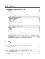
For k = 1.1 the map produces the orbits
shown in Figs. la-d. The most immediately
striking feature of this set of figures
is the existence of nontrivial structure on
all scales. Thus, like dissipative systems,
Hamiltonian chaos generates strange fractal
sets (albeit “fat” fractals, as discussed
below). On all scales one observes “islands,”
analogues in this discrete case of
the periodic orbits in the phase plane of
the simple pendulum (Fig. 2 in the main
text). In addition, however, and again on
all scales, there are swarms of dots coming
from individual chaotic orbits that undergo
nonperiodic motion and eventually
fill a finite region in phase space. In these
chaotic regions the motion is “sensitively
dependent on initial conditions.”
Figure 2 shows, in the full phase space,
a plot of a single chaotic orbit followed
through 100 million iterations (again, for
k = 1.1). This object differs from the
strange sets seen in dissipative systems in
that it occupies a finite fraction of the full
phase space: specifically, the orbit shown
takes up 56 per cent of the unit area that
represents the full phase space of the map.
Hence the “dimension” of the orbit is the
same as that of the full phase space, and
calculating the fractal dimension by the
standard method gives d f = 2. However,
the orbit differs from a conventional
area in that it contains holes on all scales.
As a consequence, the measured value of
the area occupied by the orbit depends
on the resolution with which this area is
measured—for example, the size of the
boxes in the box-counting method—and
the approach to the finite value at infinitely
fine resolution has definite scaling
properties. This set is thus appropriately
called a “fat fractal,” For our later discussion
it is important to note that the
holes—representing periodic, nonchaotic
motion—also occupy a finite fraction of
the phase space.
To develop a more intuitive feel for fat
fractals, note that a very simple example
can be constructed by using a slight
modification of the Cantor-set technique
242 Los Alamos Science Special Issue 1987

P
1.0
0.5
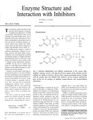
THE STANDARD MAP
Fig. 1. Shown here are the discrete orbits of
the standard map (for k = 1.1 in Eq. 1) with
different colors used to distinguish one orbit
from another. increasingly magnified regions
of the phase space are shown, starting with the
full phase space (a). The white box in (a) is the
region magnified in (b), and so forth. Nontrivial
structure, including “’islands” and swarms of
dots that represent regions of chaotic, nonperiodic
motion, are obvious on all scales. (Figure
courtesy of James Kadtke and David Umberger,
Los Alamos National Laboratory.)
0.744
P
0.719
0.4501 0.4532
0.7320
0.7289
0.694
(a)
.74
Nonlinear Science
62
0.31 0.43 0.55
0.410 0.435 0,460
q
243

Nonlinear Science
described in the main text. Instead of
deleting the middle one-third of each interval
at every scale, one deletes the mid-
sulting set is topologically the same as
the original Cantor set, a calculation of
its dimension yields d f = 1; it has the
same dimension as the full unit interval.
Further, this fat Cantor set occupies a finite
fraction-amusingly but accidentally
also about 56 per cent-of the unit interval,
with the remainder occupied by the
“holes” in the set.
To what extent does chaos exist in the
more conventional Hamiltonian systems
described by differential equations? A
full answer to this question would require
a highly technical summary of more than
eight decades of investigations by mathematical
physicists. Thus we will have
to be content with a superficial overview
that captures, at best, the flavor of these
investigations.
To begin, we note that completely integrable
systems can never exhibit chaos,
independent of the number of degrees of
freedom N. In these systems all bounded
motions are quasiperiodic and occur on
hypertori, with the N frequencies (possibly
all distinct) determined by the values
of the conservation laws. Thus there
cannot be any aperiodic motion. Further,
since all Hamiltonian systems with
N = 1 are completely integrable, chaos
cannot occur for one-degree-of-freedom
problems.
For N =2, non-integrable systems can
exhibit chaos; however, it is not trivial
to determine in which systems chaos can
occur; that :
is, it is in general not obvious
whether a given system is integrable
or not. Consider, for example, two very
similar N = 2 nonlinear Hamiltonian systems
with equation of motion given by:
244
and
d2x
Equation 2 describes the famous Henon-
Heiles system, which is non-integrable
and has become a classic example of a
simple (astro-) physically relevant Hamiltonian
system exhibiting chaos. On the
other hand, Eq. 3 can be separated into
two independent N = 1 systems (by a
tegrable.
Although there exist explicit calculational
methods for testing for integrability,
these are highly technical and generally
difficult to apply for large N. Fortunately,
two theorems provide general
guidance. First, Siegel’s Theorem considers
the space of Hamiltonians analytic
in their variables: non-integrable Hamiltonians
are dense in this space, whereas
integrable Hamiltonians are not. Second,
Nekhoroshev’s Theorem leads to the
fact that all non-integrable systems have a
phase space that contains chaotic regions.
Out observations concerning the standard
map immediately suggest an essential
question: What is the extent of the
chaotic regions and can they, under some
circumstances, cover the whole phase
space? The best way to answer this question
is to search for nonchaotic regions.
Consider, for example, a completely integrable
N-degree-of-freedom Hamiltonian
system disturbed by a generic non-integrable
perturbation. The famous KAM
(for Kolmogorov, Arnold, and Moser)
theorem shows that, for this case, there
are regions of finite measure in phase
space that retain the smoothness associated
with motion on the hypertori of the
integrable system. These regions are the
analogues of the “holes” in the standard
map. Hence, for a typical Hamiltonian
system with N degrees of freedom, the
chaotic regions do not fill all of phase
space: a finite fraction is occupied by “invariant
KAM tori.”
At a conceptual level, then, the KAM
theorem explains the nonchaotic behavior
and recurrences that so puzzled Fermi,
Pasta, and Ulam (see “The Fermi, Pasta,
and Ulam Problem: Excerpts from ‘Studies
of Nonlinear Problems’ “). Although
the FPU chain had many (64) nonlinearly
coupled degrees of freedom, it was close
enough (for the parameter ranges studied)
to an integrable system that the invariant
KAM tori and resulting pseudo-integrable
properties dominated the behavior over
the times of measurement.
There is yet another level of subtlety
to chaos in Hamiltonian systems: namely,
the structure of the phase space. For nonintegrable
systems, within every regular
KAM region there are chaotic regions.
Within these chaotic regions there are, in
turn, regular regions, and so forth. For
all non-integrable systems with N > 3,
an orbit can move (albeit on very long
time scales) among the various chaotic
regions via a process known as “Arnold
diffusion.” Thus, in general, phase space
is permeated by an Arnold web that links
together the chaotic regions on all scales.
Intuitively, these observations concerning
Hamiltonian chaos hint strongly at a
connection to statistical mechanics. As
Fig. 1 illustrates, the chaotic orbits in
Hamiltonian systems form very complicated
“Cantor dusts,” which are nonperiodic,
never-repeating motions that wander
through volumes of the phase space,
apparently constrained only by conservation
of total energy. In addition, in
these regions the sensitive dependence
implies a rapid loss of information about
the initial conditions and hence an effective
irreversibility of the motion. Clearly,
such wandering motion and effective irreversibility
suggest a possible approach
to the following fundamental question of
statistical mechanics: How can one derive
the irreversible, ergodic, thermal-
Los Alamos Science Special Issue 1987

equilibrium motion assumed in statistical
mechanics from a reversible, Hamiltonian
microscopic dynamics?
Historically, the fundamental assumption
that has linked dynamics and statistical
mechanics is the ergodic hypothesis,
which asserts that time averages over actual
dynamical motions are equal to ensemble
averages over many different but
equivalent systems. Loosely speaking,
this hypothesis assumes that all regions
of phase space allowed by energy conservation
are equally accessed by almost
all dynamical motions.
What evidence do we have that the ergodic
hypothesis actually holds for realistic
Hamiltonian systems? For systems
with finite degrees of freedom, the
KAM theorem shows that, in addition
to chaotic regions of phase space, there
are nonchaotic regions of finite measure.
These invariant tori imply that ergodicity
does not hold for most finite-dimensional
Hamiltonian sytems. Importantly, the
few Hamiltonian systems for which the
KAM theorem does not apply, and for
which one can prove ergodicity and the
approach to thermal equilibrium, involve
“hard spheres” and consequently contain
non-analytic interactions that are not realistic
from a physicist’s perspective.
For many years, most researchers believed
that these subtleties become irrelevant
in the thermodynamic limit, that is,
the limit in which the number of degrees
of freedom (N) and the energy (E) go to
infinity in such a way that E/N remains
a nonzero constant. For instance, the
KAM regions of invariant tori may approach
zero measure in this limit. However,
recent evidence suggests that nontrivial
counterexamples to this belief may
exist. Given the increasing sophistication
of our analytic understanding of Hamiltonian
chaos and the growing ability to simulate
systems with large N numerically,
the time seems ripe for quantitative investigations
that can establish (or disprove!)
this belief. (For additional discussion of
Los Alamos Science Special Issue 1987
1.0
P
0.0
0.0 1.0
this topic, see “The Ergodic Hypothesis:
A Complicated Problem of Mathematics
and Physics.”)
Among the specific issues that should
be addressed in a variety of physically
realistic models are the following.
● How does the measure of phase space
occupied by KAM tori depend on N ?
Is there a class of models with realistic
interactions for which this measure goes
to O? Are there non-integrable models
for which a finite measure is retained by
the KAM regions? If so, what are the
characteristics that cause this behavior?
● How does the rate of Arnold diffusion
depend on N in a broad class of models?
What is the structure of important
features—such as the Arnold web-in the
phase space as N approaches infinity?
● If there is an approach to equilibrium,
how does the time-scale for this approach
depend on N? Is it less than the age of
the universe?
● Is ergodicity necessary (or merely sufficient)
for most of the features we associate
with statistical mechanics? Can a
less stringent requirement, consistent with
the behaviour observed in analytic Hamiltonian
systems, be formulated?
Clearly, these are some of the most challenging,
and profound, questions currently
confronting nonlinear scientists. ■
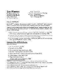
A “FAT” FRACTAL
Nonlinear Science
Fig. 2. A singles chaotic orbit of the standard
map for k = 1.1. The picture was made by dividing
the energy surface Into a 512 by 512 grid
and iterating the initial condition 10 8
times.
The squares visited by this orbit are shown
in black. Gaps in the phase space represent
portions of the energy surface unavailable to
the chaotic orbit because of various quasiperiodic
orbits confined to tori, as seen In Fig. 1.
(Figure courtesy of J. Doyne Farmer and David
Umberger, Los Alamos National Laboratory.)
245