SOLUTION FOR HOMEWORK 3, STAT 4352 Welcome to your third ...

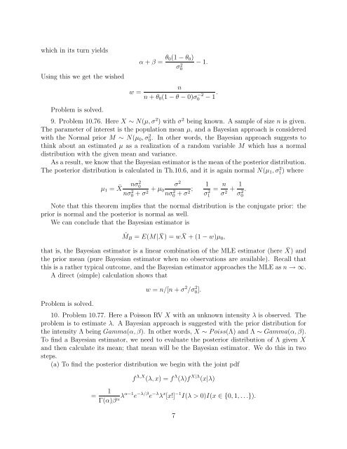
which in its turn yields
Using this we get the wished
Problem is solved.
w =
α + β = θ0(1 − θ0)
σ 2 0
− 1.
n
n + θ0(1 − θ − 0)σ −2
0 − 1 .
9. Problem 10.76. Here X ∼ N(µ, σ 2 ) with σ 2 being known. A sample of size n is given.
The parameter of interest is the population mean µ, and a Bayesian approach is considered
with the Normal prior M ∼ N(µ0, σ 2 0. In other words, the Bayesian approach suggests to
think about an estimated µ as a realization of a random variable M which has a normal
distribution with the given mean and variance.
As a result, we know that the Bayesian estimator is the mean of the posterior distribution.
The posterior distribution is calculated in Th.10.6, and it is again normal N(µ1, σ2 1 ) where
µ1 = ¯ X nσ2 0
nσ2 + µ0
0 + σ2 σ2 nσ2 0 + σ2; 1
σ 2 1
= n 1
+
σ2 σ2. 0
Note that this theorem implies that the normal distribution is the conjugate prior: the
prior is normal and the posterior is normal as well.
We can conclude that the Bayesian estimator is
ˆMB = E(M| ¯ X) = w ¯ X + (1 − w)µ0,
that is, the Bayesian estimator is a linear combination of the MLE estimator (here ¯ X) and
the prior mean (pure Bayesian estimator when no observations are available). Recall that
this is a rather typical outcome, and the Bayesian estimator approaches the MLE as n → ∞.
A direct (simple) calculation shows that
Problem is solved.
w = n/[n + σ 2 /σ 2 0 ].
10. Problem 10.77. Here a Poisson RV X with an unknown intensity λ is observed. The
problem is to estimate λ. A Bayesian approach is suggested with the prior distribution for
the intensity Λ being Gamma(α, β). In other words, X ∼ Poiss(Λ) and Λ ∼ Gamma(α, β).
To find a Bayesian estimator, we need to evaluate the posterior distribution of Λ given X
and then calculate its mean; that mean will be the Bayesian estimator. We do this in two
steps.
(a) To find the posterior distribution we begin with the joint pdf
=
f Λ,X (λ, x) = f Λ (λ)f X|Λ (x|λ)
1
Γ(α)β αλα−1 e −λ/β e −λ λ x [x!] −1 I(λ > 0)I(x ∈ {0, 1, . . .}).
7