CALCULUS I

CALCULUS I
Paul Dawkins

Calculus I
Table of Contents
Preface ........................................................................................................................................... iii
Outline ........................................................................................................................................... iv
Review............................................................................................................................................. 2
Introduction .............................................................................................................................................. 2
Review : Functions ................................................................................................................................... 4
Review : Inverse Functions .................................................................................................................... 10
Review : Trig Functions ......................................................................................................................... 17
Review : Solving Trig Equations ............................................................................................................ 24
Review : Solving Trig Equations with Calculators, Part I .................................................................... 33
Review : Solving Trig Equations with Calculators, Part II ................................................................... 44
Review : Exponential Functions ............................................................................................................ 49
Review : Logarithm Functions ............................................................................................................... 52
Review : Exponential and Logarithm Equations .................................................................................. 58
Review : Common Graphs ...................................................................................................................... 64
Limits ............................................................................................................................................ 76
Introduction ............................................................................................................................................ 76
Rates of Change and Tangent Lines ...................................................................................................... 78
The Limit ................................................................................................................................................. 87
One‐Sided Limits .................................................................................................................................... 97
Limit Properties .....................................................................................................................................103
Computing Limits ..................................................................................................................................109
Infinite Limits ........................................................................................................................................117
Limits At Infinity, Part I .........................................................................................................................126
Limits At Infinity, Part II .......................................................................................................................135
Continuity ...............................................................................................................................................144
The Definition of the Limit ....................................................................................................................151
Derivatives .................................................................................................................................. 166
Introduction ...........................................................................................................................................166
The Definition of the Derivative ...........................................................................................................168
Interpretations of the Derivative .........................................................................................................174
Differentiation Formulas ......................................................................................................................179
Product and Quotient Rule ...................................................................................................................187
Derivatives of Trig Functions ...............................................................................................................193
Derivatives of Exponential and Logarithm Functions ........................................................................204
Derivatives of Inverse Trig Functions ..................................................................................................209
Derivatives of Hyperbolic Functions ....................................................................................................215
Chain Rule ..............................................................................................................................................217
Implicit Differentiation .........................................................................................................................227
Related Rates .........................................................................................................................................236
Higher Order Derivatives ......................................................................................................................250
Logarithmic Differentiation ..................................................................................................................255
Applications of Derivatives ....................................................................................................... 258
Introduction ...........................................................................................................................................258
Rates of Change......................................................................................................................................260
Critical Points .........................................................................................................................................263
Minimum and Maximum Values ...........................................................................................................269
Finding Absolute Extrema ....................................................................................................................277
The Shape of a Graph, Part I ..................................................................................................................283
The Shape of a Graph, Part II ................................................................................................................292
The Mean Value Theorem .....................................................................................................................301
Optimization ..........................................................................................................................................308
More Optimization Problems ...............................................................................................................322
© 2007 Paul Dawkins i http://tutorial.math.lamar.edu/terms.aspx

Calculus I
Indeterminate Forms and L’Hospital’s Rule ........................................................................................336
Linear Approximations .........................................................................................................................342
Differentials ...........................................................................................................................................345
Newton’s Method ...................................................................................................................................348
Business Applications ...........................................................................................................................353
Integrals ...................................................................................................................................... 359
Introduction ...........................................................................................................................................359
Indefinite Integrals ................................................................................................................................360
Computing Indefinite Integrals ............................................................................................................366
Substitution Rule for Indefinite Integrals ............................................................................................376
More Substitution Rule .........................................................................................................................389
Area Problem .........................................................................................................................................402
The Definition of the Definite Integral .................................................................................................412
Computing Definite Integrals ...............................................................................................................422
Substitution Rule for Definite Integrals ...............................................................................................434
Applications of Integrals ........................................................................................................... 445
Introduction ...........................................................................................................................................445
Average Function Value ........................................................................................................................446
Area Between Curves ............................................................................................................................449
Volumes of Solids of Revolution / Method of Rings ............................................................................460
Volumes of Solids of Revolution / Method of Cylinders .....................................................................470
Work .......................................................................................................................................................478
Extras .......................................................................................................................................... 482
Introduction ...........................................................................................................................................482
Proof of Various Limit Properties ........................................................................................................483
Proof of Various Derivative Facts/Formulas/Properties ...................................................................494
Proof of Trig Limits ...............................................................................................................................507
Proofs of Derivative Applications Facts/Formulas .............................................................................512
Proof of Various Integral Facts/Formulas/Properties .......................................................................523
Area and Volume Formulas ..................................................................................................................535
Types of Infinity .....................................................................................................................................539
Summation Notation .............................................................................................................................543
Constants of Integration .......................................................................................................................545
© 2007 Paul Dawkins ii http://tutorial.math.lamar.edu/terms.aspx

Preface
Calculus I
Here are my online notes for my Calculus I course that I teach here at Lamar University. Despite
the fact that these are my “class notes” they should be accessible to anyone wanting to learn
Calculus I or needing a refresher in some of the early topics in calculus.
I’ve tried to make these notes as self contained as possible and so all the information needed to
read through them is either from an Algebra or Trig class or contained in other sections of the
notes.
Here are a couple of warnings to my students who may be here to get a copy of what happened on
a day that you missed.
1. Because I wanted to make this a fairly complete set of notes for anyone wanting to learn
calculus I have included some material that I do not usually have time to cover in class
and because this changes from semester to semester it is not noted here. You will need to
find one of your fellow class mates to see if there is something in these notes that wasn’t
covered in class.
2. Because I want these notes to provide some more examples for you to read through, I
don’t always work the same problems in class as those given in the notes. Likewise, even
if I do work some of the problems in here I may work fewer problems in class than are
presented here.
3. Sometimes questions in class will lead down paths that are not covered here. I try to
anticipate as many of the questions as possible when writing these up, but the reality is
that I can’t anticipate all the questions. Sometimes a very good question gets asked in
class that leads to insights that I’ve not included here. You should always talk to
someone who was in class on the day you missed and compare these notes to their notes
and see what the differences are.
4. This is somewhat related to the previous three items, but is important enough to merit its
own item. THESE NOTES ARE NOT A SUBSTITUTE FOR ATTENDING CLASS!!
Using these notes as a substitute for class is liable to get you in trouble. As already noted
not everything in these notes is covered in class and often material or insights not in these
notes is covered in class.
© 2007 Paul Dawkins iii http://tutorial.math.lamar.edu/terms.aspx

Outline
Calculus I
Here is a listing and brief description of the material in this set of notes.
Review
Review : Functions – Here is a quick review of functions, function notation and
a couple of fairly important ideas about functions.
Review : Inverse Functions – A quick review of inverse functions and the
notation for inverse functions.
Review : Trig Functions – A review of trig functions, evaluation of trig
functions and the unit circle. This section usually gets a quick review in my
class.
Review : Solving Trig Equations – A reminder on how to solve trig equations.
This section is always covered in my class.
Review : Solving Trig Equations with Calculators, Part I – The previous
section worked problem whose answers were always the “standard” angles. In
this section we work some problems whose answers are not “standard” and so a
calculator is needed. This section is always covered in my class as most trig
equations in the remainder will need a calculator.
Review : Solving Trig Equations with Calculators, Part II – Even more trig
equations requiring a calculator to solve.
Review : Exponential Functions – A review of exponential functions. This
section usually gets a quick review in my class.
Review : Logarithm Functions – A review of logarithm functions and
logarithm properties. This section usually gets a quick review in my class.
Review : Exponential and Logarithm Equations – How to solve exponential
and logarithm equations. This section is always covered in my class.
Review : Common Graphs – This section isn’t much. It’s mostly a collection
of graphs of many of the common functions that are liable to be seen in a
Calculus class.
Limits
Tangent Lines and Rates of Change – In this section we will take a look at two
problems that we will see time and again in this course. These problems will be
used to introduce the topic of limits.
The Limit – Here we will take a conceptual look at limits and try to get a grasp
on just what they are and what they can tell us.
One-Sided Limits – A brief introduction to one-sided limits.
Limit Properties – Properties of limits that we’ll need to use in computing
limits. We will also compute some basic limits in this section
© 2007 Paul Dawkins iv http://tutorial.math.lamar.edu/terms.aspx

Calculus I
Computing Limits – Many of the limits we’ll be asked to compute will not be
“simple” limits. In other words, we won’t be able to just apply the properties and
be done. In this section we will look at several types of limits that require some
work before we can use the limit properties to compute them.
Infinite Limits – Here we will take a look at limits that have a value of infinity
or negative infinity. We’ll also take a brief look at vertical asymptotes.
Limits At Infinity, Part I – In this section we’ll look at limits at infinity. In
other words, limits in which the variable gets very large in either the positive or
negative sense. We’ll also take a brief look at horizontal asymptotes in this
section. We’ll be concentrating on polynomials and rational expression
involving polynomials in this section.
Limits At Infinity, Part II – We’ll continue to look at limits at infinity in this
section, but this time we’ll be looking at exponential, logarithms and inverse
tangents.
Continuity – In this section we will introduce the concept of continuity and how
it relates to limits. We will also see the Mean Value Theorem in this section.
The Definition of the Limit – We will give the exact definition of several of the
limits covered in this section. We’ll also give the exact definition of continuity.
Derivatives
The Definition of the Derivative – In this section we will be looking at the
definition of the derivative.
Interpretation of the Derivative – Here we will take a quick look at some
interpretations of the derivative.
Differentiation Formulas – Here we will start introducing some of the
differentiation formulas used in a calculus course.
Product and Quotient Rule – In this section we will took at differentiating
products and quotients of functions.
Derivatives of Trig Functions – We’ll give the derivatives of the trig functions
in this section.
Derivatives of Exponential and Logarithm Functions – In this section we will
get the derivatives of the exponential and logarithm functions.
Derivatives of Inverse Trig Functions – Here we will look at the derivatives of
inverse trig functions.
Derivatives of Hyperbolic Functions – Here we will look at the derivatives of
hyperbolic functions.
Chain Rule – The Chain Rule is one of the more important differentiation rules
and will allow us to differentiate a wider variety of functions. In this section we
will take a look at it.
Implicit Differentiation – In this section we will be looking at implicit
differentiation. Without this we won’t be able to work some of the applications
of derivatives.
© 2007 Paul Dawkins v http://tutorial.math.lamar.edu/terms.aspx

Calculus I
Related Rates – In this section we will look at the lone application to derivatives
in this chapter. This topic is here rather than the next chapter because it will help
to cement in our minds one of the more important concepts about derivatives and
because it requires implicit differentiation.
Higher Order Derivatives – Here we will introduce the idea of higher order
derivatives.
Logarithmic Differentiation – The topic of logarithmic differentiation is not
always presented in a standard calculus course. It is presented here for those how
are interested in seeing how it is done and the types of functions on which it can
be used.
Applications of Derivatives
Rates of Change – The point of this section is to remind us of the
application/interpretation of derivatives that we were dealing with in the previous
chapter. Namely, rates of change.
Critical Points – In this section we will define critical points. Critical points
will show up in many of the sections in this chapter so it will be important to
understand them.
Minimum and Maximum Values – In this section we will take a look at some
of the basic definitions and facts involving minimum and maximum values of
functions.
Finding Absolute Extrema – Here is the first application of derivatives that
we’ll look at in this chapter. We will be determining the largest and smallest
value of a function on an interval.
The Shape of a Graph, Part I – We will start looking at the information that the
first derivatives can tell us about the graph of a function. We will be looking at
increasing/decreasing functions as well as the First Derivative Test.
The Shape of a Graph, Part II – In this section we will look at the information
about the graph of a function that the second derivatives can tell us. We will
look at inflection points, concavity, and the Second Derivative Test.
The Mean Value Theorem – Here we will take a look that the Mean Value
Theorem.
Optimization Problems – This is the second major application of derivatives in
this chapter. In this section we will look at optimizing a function, possible
subject to some constraint.
More Optimization Problems – Here are even more optimization problems.
L’Hospital’s Rule and Indeterminate Forms – This isn’t the first time that
we’ve looked at indeterminate forms. In this section we will take a look at
L’Hospital’s Rule. This rule will allow us to compute some limits that we
couldn’t do until this section.
Linear Approximations – Here we will use derivatives to compute a linear
approximation to a function. As we will see however, we’ve actually already
done this.
© 2007 Paul Dawkins vi http://tutorial.math.lamar.edu/terms.aspx

Calculus I
Differentials – We will look at differentials in this section as well as an
application for them.
Newton’s Method – With this application of derivatives we’ll see how to
approximate solutions to an equation.
Business Applications – Here we will take a quick look at some applications of
derivatives to the business field.
Integrals
Indefinite Integrals – In this section we will start with the definition of
indefinite integral. This section will be devoted mostly to the definition and
properties of indefinite integrals and we won’t be working many examples in this
section.
Computing Indefinite Integrals – In this section we will compute some
indefinite integrals and take a look at a quick application of indefinite integrals.
Substitution Rule for Indefinite Integrals – Here we will look at the
Substitution Rule as it applies to indefinite integrals. Many of the integrals that
we’ll be doing later on in the course and in later courses will require use of the
substitution rule.
More Substitution Rule – Even more substitution rule problems.
Area Problem – In this section we start off with the motivation for definite
integrals and give one of the interpretations of definite integrals.
Definition of the Definite Integral – We will formally define the definite
integral in this section and give many of its properties. We will also take a look
at the first part of the Fundamental Theorem of Calculus.
Computing Definite Integrals – We will take a look at the second part of the
Fundamental Theorem of Calculus in this section and start to compute definite
integrals.
Substitution Rule for Definite Integrals – In this section we will revisit the
substitution rule as it applies to definite integrals.
Applications of Integrals
Average Function Value – We can use integrals to determine the average value
of a function.
Area Between Two Curves – In this section we’ll take a look at determining the
area between two curves.
Volumes of Solids of Revolution / Method of Rings – This is the first of two
sections devoted to find the volume of a solid of revolution. In this section we
look that the method of rings/disks.
Volumes of Solids of Revolution / Method of Cylinders – This is the second
section devoted to finding the volume of a solid of revolution. Here we will look
at the method of cylinders.
Work – The final application we will look at is determining the amount of work
required to move an object.
© 2007 Paul Dawkins vii http://tutorial.math.lamar.edu/terms.aspx

Extras
Calculus I
Proof of Various Limit Properties – In we prove several of the limit properties
and facts that were given in various sections of the Limits chapter.
Proof of Various Derivative Facts/Formulas/Properties – In this section we
give the proof for several of the rules/formulas/properties of derivatives that we
saw in Derivatives Chapter. Included are multiple proofs of the Power Rule,
Product Rule, Quotient Rule and Chain Rule.
Proof of Trig Limits – Here we give proofs for the two limits that are needed to
find the derivative of the sine and cosine functions.
Proofs of Derivative Applications Facts/Formulas – We’ll give proofs of many
of the facts that we saw in the Applications of Derivatives chapter.
Proof of Various Integral Facts/Formulas/Properties – Here we will give the
proofs of some of the facts and formulas from the Integral Chapter as well as a
couple from the Applications of Integrals chapter.
Area and Volume Formulas – Here is the derivation of the formulas for finding
area between two curves and finding the volume of a solid of revolution.
Types of Infinity – This is a discussion on the types of infinity and how these
affect certain limits.
Summation Notation – Here is a quick review of summation notation.
Constant of Integration – This is a discussion on a couple of subtleties
involving constants of integration that many students don’t think about.
© 2007 Paul Dawkins viii http://tutorial.math.lamar.edu/terms.aspx

Calculus I
© 2007 Paul Dawkins 1 http://tutorial.math.lamar.edu/terms.aspx

Review
Introduction
Calculus I
Technically a student coming into a Calculus class is supposed to know both Algebra and
Trigonometry. The reality is often much different however. Most students enter a Calculus class
woefully unprepared for both the algebra and the trig that is in a Calculus class. This is very
unfortunate since good algebra skills are absolutely vital to successfully completing any Calculus
course and if your Calculus course includes trig (as this one does) good trig skills are also
important in many sections.
The intent of this chapter is to do a very cursory review of some algebra and trig skills that are
absolutely vital to a calculus course. This chapter is not inclusive in the algebra and trig skills
that are needed to be successful in a Calculus course. It only includes those topics that most
students are particularly deficient in. For instance factoring is also vital to completing a standard
calculus class but is not included here. For a more in depth review you should visit my
Algebra/Trig review or my full set of Algebra notes at http://tutorial.math.lamar.edu.
Note that even though these topics are very important to a Calculus class I rarely cover all of
these in the actual class itself. We simply don’t have the time to do that. I do cover certain
portions of this chapter in class, but for the most part I leave it to the students to read this chapter
on their own.
Here is a list of topics that are in this chapter. I’ve also denoted the sections that I typically cover
during the first couple of days of a Calculus class.
Review : Functions – Here is a quick review of functions, function notation and a couple of
fairly important ideas about functions.
Review : Inverse Functions – A quick review of inverse functions and the notation for inverse
functions.
Review : Trig Functions – A review of trig functions, evaluation of trig functions and the unit
circle. This section usually gets a quick review in my class.
Review : Solving Trig Equations – A reminder on how to solve trig equations. This section is
always covered in my class.
© 2007 Paul Dawkins 2 http://tutorial.math.lamar.edu/terms.aspx

Calculus I
Review : Solving Trig Equations with Calculators, Part I – The previous section worked
problem whose answers were always the “standard” angles. In this section we work some
problems whose answers are not “standard” and so a calculator is needed. This section is always
covered in my class as most trig equations in the remainder will need a calculator.
Review : Solving Trig Equations with Calculators, Part II – Even more trig equations
requiring a calculator to solve.
Review : Exponential Functions – A review of exponential functions. This section usually gets
a quick review in my class.
Review : Logarithm Functions – A review of logarithm functions and logarithm properties.
This section usually gets a quick review in my class.
Review : Exponential and Logarithm Equations – How to solve exponential and logarithm
equations. This section is always covered in my class.
Review : Common Graphs – This section isn’t much. It’s mostly a collection of graphs of many
of the common functions that are liable to be seen in a Calculus class.
© 2007 Paul Dawkins 3 http://tutorial.math.lamar.edu/terms.aspx

Review : Functions
Calculus I
In this section we’re going to make sure that you’re familiar with functions and function notation.
Both will appear in almost every section in a Calculus class and so you will need to be able to
deal with them.
First, what exactly is a function? An equation will be a function if for any x in the domain of the
equation (the domain is all the x’s that can be plugged into the equation) the equation will yield
exactly one value of y.
This is usually easier to understand with an example.
Example 1 Determine if each of the following are functions.
2
(a) y = x + 1
2
(b) y = x + 1
Solution
(a) This first one is a function. Given an x there is only one way to square it and then add 1 to the
result and so no matter what value of x you put into the equation there is only one possible value
of y.
(b) The only difference between this equation and the first is that we moved the exponent off the
x and onto the y. This small change is all that is required, in this case, to change the equation
from a function to something that isn’t a function.
To see that this isn’t a function is fairly simple. Choose a value of x, say x=3 and plug this into
the equation.
2
y = 3+ 1= 4
Now, there are two possible values of y that we could use here. We could use y = 2 or y =− 2 .
Since there are two possible values of y that we get from a single x this equation isn’t a function.
Note that this only needs to be the case for a single value of x to make an equation not be a
function. For instance we could have used x=-1 and in this case we would get a single y (y=0).
However, because of what happens at x=3 this equation will not be a function.
Next we need to take a quick look at function notation. Function notation is nothing more than a
fancy way of writing the y in a function that will allow us to simplify notation and some of our
work a little.
Let’s take a look at the following function.
2
y = 2x − 5x+ 3
Using function notation we can write this as any of the following.
© 2007 Paul Dawkins 4 http://tutorial.math.lamar.edu/terms.aspx

Calculus I
( ) ( )
( ) ( )
( ) ( )
f x = x − x+ g x = x − x+
2 2
2 5 3 2 5 3
h x = x − x+ R x = x − x+
2 2
2 5 3 2 5 3
w x = x − x+ y x = x − x+
2 2
2 5 3 2 5 3
Recall that this is NOT a letter times x, this is just a fancy way of writing y.
So, why is this useful? Well let’s take the function above and let’s get the value of the function at
x=-3. Using function notation we represent the value of the function at x=-3 as f(-3). Function
notation gives us a nice compact way of representing function values.
Now, how do we actually evaluate the function? That’s really simple. Everywhere we see an x
on the right side we will substitute whatever is in the parenthesis on the left side. For our
function this gives,
2
f ( − 3) = 2( −3) −5( − 3) + 3
= 29 ( ) + 15+ 3
= 36
Let’s take a look at some more function evaluation.
2
Example 2 Given f ( x) =− x + 6x− 11 find each of the following.
(a) f ( 2)
[Solution]
Solution
(b) f ( − 10)
[Solution]
(c) f () t [Solution]
(d) f ( t− 3)
[Solution]
(e) f ( x− 3)
[Solution]
(f) f ( 4x− 1)
[Solution]
(a) ( ) ( ) 2
f 2 =− 2 + 6(2) − 11 =− 3
2
(b) ( ) ( ) ( )
f − 10 =− − 10 + 6 −10 − 11 =−100 −60 − 11 =− 171
Be careful when squaring negative numbers!
2
(c) f () t =− t + 6t− 11
[Return to Problems]
[Return to Problems]
Remember that we substitute for the x’s WHATEVER is in the parenthesis on the left. Often this
will be something other than a number. So, in this case we put t’s in for all the x’s on the left.
[Return to Problems]
© 2007 Paul Dawkins 5 http://tutorial.math.lamar.edu/terms.aspx

2 2
(d) ( ) ( ) ( )
Calculus I
f t− 3 =− t− 3 + 6 t−3− 11 =− t + 12t− 38
Often instead of evaluating functions at numbers or single letters we will have some fairly
complex evaluations so make sure that you can do these kinds of evaluations.
[Return to Problems]
2 2
f x− 3 =− x− 3 + 6 x−3− 11 =− x + 12x− 38
The only difference between this one and the previous one is that I changed the t to an x. Other
than that there is absolutely no difference between the two! Don’t get excited if an x appears
inside the parenthesis on the left.
[Return to Problems]
(e) ( ) ( ) ( )
(f) ( ) ( ) ( )
2 2
f 4x− 1 =− 4x− 1 + 6 4x−1 − 11=− 16x + 32x− 18
This one is not much different from the previous part. All we did was change the equation that
we were plugging into function.
[Return to Problems]
All throughout a calculus course we will be finding roots of functions. A root of a function is
nothing more than a number for which the function is zero. In other words, finding the roots of a
function, g(x), is equivalent to solving
g( x ) = 0
Example 3 Determine all the roots of ( ) 3 2
Solution
So we will need to solve,
f t = 9t − 18t + 6t
3 2
9t − 18t + 6t = 0
First, we should factor the equation as much as possible. Doing this gives,
3t 2
3t − 6t+ 2 = 0
( )
Next recall that if a product of two things are zero then one (or both) of them had to be zero. This
means that,
3t= 0 OR,
2
3t − 6t+ 2= 0
From the first it’s clear that one of the roots must then be t=0. To get the remaining roots we will
need to use the quadratic formula on the second equation. Doing this gives,
© 2007 Paul Dawkins 6 http://tutorial.math.lamar.edu/terms.aspx

Calculus I
( 6) (
2
6) 4( 3)( 2)
23 ( )
− − ± − −
t =
6± 12
=
6
6± =
4
6
3
6± 2 3
=
6
3± 3
=
3
1
= 1± 3
3
= 1±
1
3
( )( )
In order to remind you how to simplify radicals we gave several forms of the answer.
To complete the problem, here is a complete list of all the roots of this function.
3+ 3 3− 3
t = 0, t = , t =
3 3
Note we didn’t use the final form for the roots from the quadratic. This is usually where we’ll
stop with the simplification for these kinds of roots. Also note that, for the sake of the practice,
we broke up the compact form for the two roots of the quadratic. You will need to be able to do
this so make sure that you can.
This example had a couple of points other than finding roots of functions.
The first was to remind you of the quadratic formula. This won’t be the first time that you’ll need
it in this class.
The second was to get you used to seeing “messy” answers. In fact, the answers in the above list
are not that messy. However, most students come out of an Algebra class very used to seeing
only integers and the occasional “nice” fraction as answers.
So, here is fair warning. In this class I often will intentionally make the answers look “messy”
just to get you out of the habit of always expecting “nice” answers. In “real life” (whatever that
is) the answer is rarely a simple integer such as two. In most problems the answer will be a
decimal that came about from a messy fraction and/or an answer that involved radicals.
© 2007 Paul Dawkins 7 http://tutorial.math.lamar.edu/terms.aspx

Calculus I
The next topic that we need to discuss here is that of function composition. The composition of
f(x) and g(x) is
( f g)( x) = f ( g( x)
)
In other words, compositions are evaluated by plugging the second function listed into the first
function listed. Note as well that order is important here. Interchanging the order will usually
result in a different answer.
Example 4 Given
2
f ( x) = 3x − x+
10 and ( ) 1 20
(a) ( f g)(
5)
[Solution]
Solution
f g
(a) ( )( 5)
(b) ( f g)( x)
[Solution]
(c) ( g f )( x)
[Solution]
(d) ( g g)( x)
[Solution]
g x = − x find each of the following.
In this case we’ve got a number instead of an x but it works in exactly the same way.
f g 5 = f g 5
(b) ( f g)( x)
( )
( )( ) ( )
f ( )
= − 99 = 29512
( f g)( x) = f ( g( x)
)
= f ( 1−20x) 2
( x) ( x)
= 31−20− 1− 20 + 10
2
( )
= 3 1− 40x+ 400x − 1+ 20x+ 10
[Return to Problems]
2
= 1200x − 100x+ 12
Compare this answer to the next part and notice that answers are NOT the same. The order in
which the functions are listed is important!
[Return to Problems]
(c) ( g f )( x)
( gf )( x) = g f ( x)
( )
( 3
2
10)
( 2
x x )
= g x − x+
= 1−20 3 − + 10
2
= − 60x + 20x −199
And just to make the point. This answer is different from the previous part. Order is important in
composition.
[Return to Problems]
© 2007 Paul Dawkins 8 http://tutorial.math.lamar.edu/terms.aspx

Calculus I
(d) ( g g)( x)
In this case do not get excited about the fact that it’s the same function. Composition still works
the same way.
gg x = g g x
( )
( )( ) ( )
= g( 1−20x) = 1−20( 1−20x) = 400x −19
Let’s work one more example that will lead us into the next section.
Example 5 Given f ( x) = 3x− 2 and ( )
(a) ( f g)( x)
(b) ( g f )( x)
Solution
(a)
(b)
1 2
g x = x+
find each of the following.
3 3
( )
( f g)( x) = f g( x)
⎛1 2⎞
= f ⎜ x+
⎟
⎝3 3⎠
⎛1 2⎞
= 3⎜ x + ⎟−2
⎝3 3⎠
= x + 2− 2=
x
( )
( gf )( x) = g f ( x)
= g( 3x−2) 1 2
= ( 3x− 2)
+
3 3
2 2
= x − + = x
3 3
[Return to Problems]
In this case the two compositions where the same and in fact the answer was very simple.
( f g)( x) = ( g f )( x) = x
This will usually not happen. However, when the two compositions are the same, or more
specifically when the two compositions are both x there is a very nice relationship between the
two functions. We will take a look at that relationship in the next section.
© 2007 Paul Dawkins 9 http://tutorial.math.lamar.edu/terms.aspx

Review : Inverse Functions
Calculus I
In the last example from the previous section we looked at the two functions f ( x) = 3x− 2 and
x 2
g( x ) = + and saw that
3 3
( f g)( x) = ( g f )( x) = x
and as noted in that section this means that there is a nice relationship between these two
functions. Let’s see just what that relationship is. Consider the following evaluations.
−5 2 −3
f ( −1)
= 3( −1) − 2=
−5 ⇒ g(
−5)
= + = = −1
3 3 3
2 2 4 ⎛4⎞ ⎛4⎞ g( 2) = + = ⇒ f ⎜ ⎟= 3⎜ ⎟−
2= 4− 2=
2
3 3 3 ⎝3⎠ ⎝3⎠
In the first case we plugged x =− 1 into f ( x ) and got a value of -5. We then turned around and
plugged x =− 5 into g( x ) and got a value of -1, the number that we started off with.
In the second case we did something similar. Here we plugged x = 2 into g( x ) and got a value
, we turned around and plugged this into f ( x ) and got a value of 2, which is again the
of 4
3
number that we started with.
Note that we really are doing some function composition here. The first case is really,
( g f )( − 1) = g⎡⎣f ( − 1) ⎤⎦
= g[
− 5] =−1
and the second case is really,
⎡4⎤ ( f g)( 2) = f ⎡⎣g( 2) ⎤⎦
= f
⎢
= 2
⎣3⎥ ⎦
Note as well that these both agree with the formula for the compositions that we found in the
previous section. We get back out of the function evaluation the number that we originally
plugged into the composition.
So, just what is going on here? In some way we can think of these two functions as undoing what
the other did to a number. In the first case we plugged x = − 1 into f ( x ) and then plugged the
result from this function evaluation back into g( x ) and in some way g( x ) undid what f ( x )
had done to x =− 1 and gave us back the original x that we started with.
© 2007 Paul Dawkins 10 http://tutorial.math.lamar.edu/terms.aspx

Calculus I
Function pairs that exhibit this behavior are called inverse functions. Before formally defining
inverse functions and the notation that we’re going to use for them we need to get a definition out
of the way.
A function is called one-to-one if no two values of x produce the same y. Mathematically this is
the same as saying,
f x ≠ f x whenever x ≠ x
( ) ( )
1 2 1 2
So, a function is one-to-one if whenever we plug different values into the function we get
different function values.
Sometimes it is easier to understand this definition if we see a function that isn’t one-to-one.
Let’s take a look at a function that isn’t one-to-one. The function
2
f ( x) = x is not one-to-one
because both f ( − 2) = 4 and ( 2) 4
f = . In other words there are two different values of x that
2
produce the same value of y. Note that we can turn f ( x) = x into a one-to-one function if we
restrict ourselves to 0 ≤ x

Calculus I
Now, be careful with the notation for inverses. The “-1” is NOT an exponent despite the fact that
is sure does look like one! When dealing with inverse functions we’ve got to remember that
−1
1
f ( x)
≠
f ( x)
This is one of the more common mistakes that students make when first studying inverse
functions.
The process for finding the inverse of a function is a fairly simple one although there are a couple
of steps that can on occasion be somewhat messy. Here is the process
Finding the Inverse of a Function
−1
Given the function f ( x ) we want to find the inverse function, f ( x)
.
1. First, replace f ( x ) with y. This is done to make the rest of the process easier.
2. Replace every x with a y and replace every y with an x.
3. Solve the equation from Step 2 for y. This is the step where mistakes are most often
made so be careful with this step.
−1
4. Replace y with f ( x)
. In other words, we’ve managed to find the inverse at this point!
−1
−1
5. Verify your work by checking that ( f f )( x) = x and ( f f )( x) = x are both
true. This work can sometimes be messy making it easy to make mistakes so again be
careful.
That’s the process. Most of the steps are not all that bad but as mentioned in the process there are
a couple of steps that we really need to be careful with since it is easy to make mistakes in those
steps.
−1
In the verification step we technically really do need to check that both ( f f )( x) = x and
−1
( )( )
f f x = x are true. For all the functions that we are going to be looking at in this course
if one is true then the other will also be true. However, there are functions (they are beyond the
scope of this course however) for which it is possible for only one of these to be true. This is
brought up because in all the problems here we will be just checking one of them. We just need
to always remember that technically we should check both.
Let’s work some examples.
−1
Example 1 Given f ( x) = 3x− 2 find f ( x)
Solution
Now, we already know what the inverse to this function is as we’ve already done some work with
it. However, it would be nice to actually start with this since we know what we should get. This
will work as a nice verification of the process.
© 2007 Paul Dawkins 12 http://tutorial.math.lamar.edu/terms.aspx
.

Calculus I
So, let’s get started. We’ll first replace f ( x ) with y.
y = 3x− 2
Next, replace all x’s with y and all y’s with x.
x= 3y− 2
Now, solve for y.
−1
Finally replace y with f ( x)
.
1
3
x + 2= 3y
( 2)
x + = y
x 2
+ = y
3 3
( )
−1
f x
x 2
= +
3 3
Now, we need to verify the results. We already took care of this in the previous section, however,
we really should follow the process so we’ll do that here. It doesn’t matter which of the two that
−1
we check we just need to check one of them. This time we’ll check that ( f f )( x) = x is
true.
−1 −1
( f f )( x) f f ( x)
−1
Example 2 Given g( x) = x−
3 find g ( x)
= ⎡
⎣
⎤
⎦
⎡ x 2⎤
= f
⎢
+
⎣ 3 3⎥
⎦
⎛ x 2 ⎞
= 3⎜ + ⎟−2
⎝3 3⎠
= x + 2−2 = x
Solution
The fact that we’re using g( x ) instead of f ( x ) doesn’t change how the process works. Here
are the first few steps.
© 2007 Paul Dawkins 13 http://tutorial.math.lamar.edu/terms.aspx
.
y = x−3
x= y−
3

Calculus I
Now, to solve for y we will need to first square both sides and then proceed as normal.
x= y−3
This inverse is then,
2
x y
2
x + 3 = y
( )
= −3
g x x
−1
2
= + 3
Finally let’s verify and this time we’ll use the other one just so we can say that we’ve gotten both
down somewhere in an example.
−1 −1
( g g)( x) g g( x)
= ⎡⎣ ⎤⎦
−1
g ( x 3)
( x
2
)
= −
= − 3 + 3
= x − 3+ 3
= x
So, we did the work correctly and we do indeed have the inverse.
The next example can be a little messy so be careful with the work here.
x + 4
−1
Example 3 Given h( x)
= find h ( x)
.
2x− 5
Solution
The first couple of steps are pretty much the same as the previous examples so here they are,
x + 4
y =
2x−5 y + 4
x =
2y−5 Now, be careful with the solution step. With this kind of problem it is very easy to make a
mistake here.
© 2007 Paul Dawkins 14 http://tutorial.math.lamar.edu/terms.aspx

Calculus I
( )
x 2y− 5 = y+
4
2xy − 5x= y + 4
2xy− y = 4+ 5x
( 2x− 1) y = 4+ 5x
4+ 5x
y =
2x−1 So, if we’ve done all of our work correctly the inverse should be,
− 1 4+ 5x
h ( x)
=
2x− 1
Finally we’ll need to do the verification. This is also a fairly messy process and it doesn’t really
matter which one we work with.
−1 −1
( hh )( x) = h⎡ ⎣h ( x)
⎤
⎦
⎡4+ 5x⎤
= h
⎢
⎣2x−1⎥ ⎦
4+ 5x
+ 4
= 2x−1 ⎛4+ 5x⎞
2⎜ ⎟−5
⎝ 2x−1⎠ Okay, this is a mess. Let’s simplify things up a little bit by multiplying the numerator and
denominator by 2x− 1.
4+ 5x
+ 4
−1
2x−1 ( hh )( x)
= 2x−1 2x−1 ⎛4+ 5x⎞
2⎜ ⎟−5
⎝ 2x−1⎠ ⎛4+ 5x
⎞
( 2x− 1) ⎜ + 4⎟
2x−1 =
⎝ ⎠
⎛ ⎛4+ 5x⎞
⎞
( 2x−1) ⎜2⎜ ⎟−5
2x1 ⎟
⎝ ⎝ − ⎠ ⎠
4+ 5x+ 4( 2x−1) =
2( 4+ 5x) −5( 2x−1) 4+ 5x+ 8x−4 =
8+ 10x− 10x+ 5
13x
= = x
13
Wow. That was a lot of work, but it all worked out in the end. We did all of our work correctly
and we do in fact have the inverse.
© 2007 Paul Dawkins 15 http://tutorial.math.lamar.edu/terms.aspx

Calculus I
There is one final topic that we need to address quickly before we leave this section. There is an
interesting relationship between the graph of a function and the graph of its inverse.
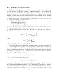
Here is the graph of the function and inverse from the first two examples.
In both cases we can see that the graph of the inverse is a reflection of the actual function about
the line y = x . This will always be the case with the graphs of a function and its inverse.
© 2007 Paul Dawkins 16 http://tutorial.math.lamar.edu/terms.aspx

Review : Trig Functions
Calculus I
The intent of this section is to remind you of some of the more important (from a Calculus
standpoint…) topics from a trig class. One of the most important (but not the first) of these topics
will be how to use the unit circle. We will actually leave the most important topic to the next
section.
First let’s start with the six trig functions and how they relate to each other.
( x) ( x)
( x) ( )
( )
( x)
cos sin
tan
sin
=
cos
x
x
cot
cos
=
sin
x
x
1
=
tan x
1
sec( x) =
cos x
1
csc(
x)
=
sin x
( )
( )
( ) ( )
Recall as well that all the trig functions can be defined in terms of a right triangle.
From this right triangle we get the following definitions of the six trig functions.
adjacent
cosθ
=
hypotenuse
opposite
tanθ
=
adjacent
hypotenuse
secθ
=
adjacent
© 2007 Paul Dawkins 17 http://tutorial.math.lamar.edu/terms.aspx
( )
opposite
sinθ
=
hypotenuse
adjacent
cotθ
=
opposite
hypotenuse
cscθ
=
opposite
Remembering both the relationship between all six of the trig functions and their right triangle
definitions will be useful in this course on occasion.
Next, we need to touch on radians. In most trig classes instructors tend to concentrate on doing
everything in terms of degrees (probably because it’s easier to visualize degrees). The same is

Calculus I
true in many science classes. However, in a calculus course almost everything is done in radians.
The following table gives some of the basic angles in both degrees and radians.
Degree 0 30 45 60 90 180 270 360
Radians 0
π
6
π
4
π
3
π
2
π
3π
2
2π
Know this table! We may not see these specific angles all that much when we get into the
Calculus portion of these notes, but knowing these can help us to visualize each angle. Now, one
more time just make sure this is clear.
Be forewarned, everything in most calculus classes will be done in radians!
Let’s next take a look at one of the most overlooked ideas from a trig class. The unit circle is one
of the more useful tools to come out of a trig class. Unfortunately, most people don’t learn it as
well as they should in their trig class.
Below is the unit circle with just the first quadrant filled in. The way the unit circle works is to
draw a line from the center of the circle outwards corresponding to a given angle. Then look at
the coordinates of the point where the line and the circle intersect. The first coordinate is the
cosine of that angle and the second coordinate is the sine of that angle. We’ve put some of the
basic angles along with the coordinates of their intersections on the unit circle. So, from the unit
⎛π⎞ 3 ⎛π⎞ 1
circle below we can see that cos⎜ ⎟=
and sin ⎜ ⎟=
.
⎝ 6 ⎠ 2 ⎝ 6 ⎠ 2
© 2007 Paul Dawkins 18 http://tutorial.math.lamar.edu/terms.aspx

Calculus I
Remember how the signs of angles work. If you rotate in a counter clockwise direction the angle
is positive and if you rotate in a clockwise direction the angle is negative.
Recall as well that one complete revolution is 2π , so the positive x-axis can correspond to either
an angle of 0 or 2π (or 4π , or 6π , or − 2π , or − 4π , etc. depending on the direction of
rotation). Likewise, the angle π
6 (to pick an angle completely at random) can also be any of the
following angles:
In fact 6
π 13π
π
+ 2π
= (start at then rotate once around counter clockwise)
6 6 6
π 25π
π
+ 4π
= (start at then rotate around twice counter clockwise)
6 6 6
π 11π
π
− 2π
=− (start at then rotate once around clockwise)
6 6 6
π 23π
π
− 4π
=− (start at then rotate around twice clockwise)
6 6 6
etc.
π can be any of the following angles 6 2 , 0, 1, 2, 3,
π π
+ n n=
± ± ± … In this case n is
the number of complete revolutions you make around the unit circle starting at π
6 . Positive
values of n correspond to counter clockwise rotations and negative values of n correspond to
clockwise rotations.
So, why did I only put in the first quadrant? The answer is simple. If you know the first quadrant
then you can get all the other quadrants from the first with a small application of geometry.
You’ll see how this is done in the following set of examples.
Example 1 Evaluate each of the following.
⎛2π⎞ (a) sin ⎜ ⎟
⎝ 3 ⎠ and
⎛ 2π
⎞
sin ⎜−⎟ ⎝ 3 ⎠ [Solution]
⎛7π⎞ (b) cos⎜
⎟
⎝ 6 ⎠ and
⎛ 7π
⎞
cos⎜−⎟
⎝ 6 ⎠ [Solution]
⎛ π ⎞
(c) tan ⎜−⎟ ⎝ 4 ⎠ and
⎛7π⎞ tan ⎜ ⎟
⎝ 4 ⎠ [Solution]
⎛25π ⎞
(d) sec⎜
⎟
⎝ 6 ⎠ [Solution]
© 2007 Paul Dawkins 19 http://tutorial.math.lamar.edu/terms.aspx

Calculus I
Solution
(a) The first evaluation in this part uses the angle 2π
. That’s not on our unit circle above,
3
however notice that 2π
π
= π − . So
3 3
2π
π
is found by rotating up from the negative x-axis.
3
3
This means that the line for 2π
π
will be a mirror image of the line for only in the second
3
3
quadrant. The coordinates for 2π
π
will be the coordinates for except the x coordinate will be
3
3
negative.
Likewise for 2π
− we can notice that
3
2π
π
− =− π + , so this angle can be found by rotating
3 3
π 2π
down from the negative x-axis. This means that the line for − will be a mirror image of
3
3
π
the line for only in the third quadrant and the coordinates will be the same as the coordinates
3
π
for except both will be negative.
3
Both of these angles along with their coordinates are shown on the following unit circle.
⎛2π⎞ 3 ⎛ 2π⎞ 3
From this unit circle we can see that sin ⎜ ⎟=
and sin ⎜− ⎟=−
.
⎝ 3 ⎠ 2 ⎝ 3 ⎠ 2
© 2007 Paul Dawkins 20 http://tutorial.math.lamar.edu/terms.aspx

Calculus I
This leads to a nice fact about the sine function. The sine function is called an odd function and
so for ANY angle we have
sin ( − θ ) =− sin ( θ )
[Return to Problems]
(b) For this example notice that 7π
π
π
= π + so this means we would rotate down from the
6 6
6
negative x-axis to get to this angle. Also 7π
π
π
− =−π − so this means we would rotate up
6 6
6
from the negative x-axis to get to this angle. So, as with the last part, both of these angles will be
π
mirror images of in the third and second quadrants respectively and we can use this to
6
determine the coordinates for both of these new angles.
Both of these angles are shown on the following unit circle along with appropriate coordinates for
the intersection points.
⎛7π⎞ From this unit circle we can see that cos⎜
⎟=−
⎝ 6 ⎠
3 ⎛ 7π⎞ and cos⎜−
⎟=−
2 ⎝ 6 ⎠
3
. In this case
2
the cosine function is called an even function and so for ANY angle we have
( θ ) ( θ )
cos − = cos .
[Return to Problems]
© 2007 Paul Dawkins 21 http://tutorial.math.lamar.edu/terms.aspx

Calculus I
(c) Here we should note that 7π
π
= 2π
− so
4 4
7π
π
and − are in fact the same angle! Also
4 4
π
note that this angle will be the mirror image of in the fourth quadrant. The unit circle for this
4
angle is
Now, if we remember that tan ( x)
tangent function. So,
( x)
( x)
sin
= we can use the unit circle to find the values the
cos
( π )
( −π
)
⎛7π ⎞ ⎛ π ⎞ sin − 4 − 2 2
tan ⎜ ⎟= tan ⎜− ⎟=
= =−1.
⎝ 4 ⎠ ⎝ 4 ⎠ cos 4 22
⎛π⎞ On a side note, notice that tan ⎜ ⎟=
1 and we can see that the tangent function is also called an
⎝ 4 ⎠
odd function and so for ANY angle we will have
( θ ) ( θ )
tan − =− tan .
[Return to Problems]
(d) Here we need to notice that 25π
π
π
= 4π
+ . In other words, we’ve started at and rotated
6 6
6
around twice to end back up at the same point on the unit circle. This means that
⎛25π ⎞ ⎛ π ⎞ ⎛π ⎞
sec⎜ ⎟= sec⎜4π+ ⎟= sec⎜
⎟
⎝ 6 ⎠ ⎝ 6 ⎠ ⎝ 6 ⎠
© 2007 Paul Dawkins 22 http://tutorial.math.lamar.edu/terms.aspx

Calculus I
Now, let’s also not get excited about the secant here. Just recall that
1
sec(
x)
=
cos ( x)
and so all we need to do here is evaluate a cosine! Therefore,
⎛25π ⎞ ⎛π ⎞ 1 1 2
sec⎜ ⎟= sec⎜
⎟=
= =
⎝ 6 ⎠ ⎝ 6 ⎠ ⎛π⎞ cos
3 3
⎜ ⎟
⎝ 6 ⎠
2
[Return to Problems]
So, in the last example we saw how the unit circle can be used to determine the value of the trig
functions at any of the “common” angles. It’s important to notice that all of these examples used
the fact that if you know the first quadrant of the unit circle and can relate all the other angles to
“mirror images” of one of the first quadrant angles you don’t really need to know whole unit
circle. If you’d like to see a complete unit circle I’ve got one on my Trig Cheat Sheet that is
available at http://tutorial.math.lamar.edu.
Another important idea from the last example is that when it comes to evaluating trig functions all
that you really need to know is how to evaluate sine and cosine. The other four trig functions are
defined in terms of these two so if you know how to evaluate sine and cosine you can also
evaluate the remaining four trig functions.
We’ve not covered many of the topics from a trig class in this section, but we did cover some of
the more important ones from a calculus standpoint. There are many important trig formulas that
you will use occasionally in a calculus class. Most notably are the half-angle and double-angle
formulas. If you need reminded of what these are, you might want to download my Trig Cheat
Sheet as most of the important facts and formulas from a trig class are listed there.
© 2007 Paul Dawkins 23 http://tutorial.math.lamar.edu/terms.aspx

Review : Solving Trig Equations
Calculus I
In this section we will take a look at solving trig equations. This is something that you will be
asked to do on a fairly regular basis in my class.
Let’s just jump into the examples and see how to solve trig equations.
Example 1 Solve 2cos() t = 3.
Solution
There’s really not a whole lot to do in solving this kind of trig equation. All we need to do is
divide both sides by 2 and the go to the unit circle.
2cos t = 3
cos
( )
() t
So, we are looking for all the values of t for which cosine will have the value of 3
. So, let’s
2
take a look at the following unit circle.
From quick inspection we can see that
© 2007 Paul Dawkins 24 http://tutorial.math.lamar.edu/terms.aspx
=
3
2
t
6
π
= is a solution. However, as I have shown on the unit

Calculus I
circle there is another angle which will also be a solution. We need to determine what this angle
is. When we look for these angles we typically want positive angles that lie between 0 and 2π .
This angle will not be the only possibility of course, but by convention we typically look for
angles that meet these conditions.
To find this angle for this problem all we need to do is use a little geometry. The angle in the first
π
quadrant makes an angle of with the positive x-axis, then so must the angle in the fourth
6
π
quadrant. So we could use − , but again, it’s more common to use positive angles so, we’ll use
6
π 11π
t = 2π
− = .
6 6
We aren’t done with this problem. As the discussion about finding the second angle has shown
π
there are many ways to write any given angle on the unit circle. Sometimes it will be − that
6
we want for the solution and sometimes we will want both (or neither) of the listed angles.
Therefore, since there isn’t anything in this problem (contrast this with the next problem) to tell
us which is the correct solution we will need to list ALL possible solutions.
This is very easy to do. Recall from the previous section and you’ll see there that I used
π
+ 2 π n, n=
0, ± 1, ± 2, ± 3, …
6
to represent all the possible angles that can end at the same location on the unit circle, i.e. angles
π π
that end at . Remember that all this says is that we start at then rotate around in the
6
6
counter-clockwise direction (n is positive) or clockwise direction (n is negative) for n complete
rotations. The same thing can be done for the second solution.
So, all together the complete solution to this problem is
π
+ 2 π n, n=
0, ± 1, ± 2, ± 3, …
6
11π
+ 2 π n, n=
0, ± 1, ± 2, ± 3, …
6
π
As a final thought, notice that we can get − by using n = − 1 in the second solution.
6
Now, in a calculus class this is not a typical trig equation that we’ll be asked to solve. A more
typical example is the next one.
© 2007 Paul Dawkins 25 http://tutorial.math.lamar.edu/terms.aspx

Calculus I
Example 2 Solve 2cos() t = 3 on [ − 2 π ,2 π ] .
Solution
In a calculus class we are often more interested in only the solutions to a trig equation that fall in
a certain interval. The first step in this kind of problem is to first find all possible solutions. We
did this in the first example.
π
+ 2 π n, n=
0, ± 1, ± 2, ± 3, …
6
11π
+ 2 π n, n=
0, ± 1, ± 2, ± 3, …
6
Now, to find the solutions in the interval all we need to do is start picking values of n, plugging
them in and getting the solutions that will fall into the interval that we’ve been given.
n=0.
π π
+ 2π( 0) = < 2π
6 6
11π 11π
+ 2π( 0) = < 2π
6 6
Now, notice that if we take any positive value of n we will be adding on positive multiples of 2π
onto a positive quantity and this will take us past the upper bound of our interval and so we don’t
need to take any positive value of n.
However, just because we aren’t going to take any positive value of n doesn’t mean that we
shouldn’t also look at negative values of n.
n=-1.
π 11π
+ 2π( − 1) =− >−2π
6 6
11π
π
+ 2π( − 1) =− >−2π
6 6
These are both greater than −2π and so are solutions, but if we subtract another 2π off (i.e use
n =− 2 ) we will once again be outside of the interval so we’ve found all the possible solutions
that lie inside the interval [ − 2 π ,2 π ] .
π 11π π 11π
So, the solutions are : , , − , − .
6 6 6 6
So, let’s see if you’ve got all this down.
© 2007 Paul Dawkins 26 http://tutorial.math.lamar.edu/terms.aspx

Example 3 Solve 2sin( 5 ) 3
Calculus I
x =− on [ − π ,2 π ]
Solution
This problem is very similar to the other problems in this section with a very important
difference. We’ll start this problem in exactly the same way. We first need to find all possible
solutions.
2sin(5 x)
=− 3
− 3
sin(5 x)
=
2
3
So, we are looking for angles that will give − out of the sine function. Let’s again go to our
2
trusty unit circle.
Now, there are no angles in the first quadrant for which sine has a value of −
3
. However,
2
there are two angles in the lower half of the unit circle for which sine will have a value of −
3
.
2
⎛π⎞ So, what are these angles? We’ll notice sin ⎜ ⎟=
⎝ 3⎠ 3
, so the angle in the third quadrant will be
2
© 2007 Paul Dawkins 27 http://tutorial.math.lamar.edu/terms.aspx

Calculus I
π π 4π
π
below the negative x-axis or π + = . Likewise, the angle in the fourth quadrant will
3
3 3
3
π 5π
below the positive x-axis or 2π
− = . Remember that we’re typically looking for positive
3 3
angles between 0 and 2π .
Now we come to the very important difference between this problem and the previous problems
in this section. The solution is NOT
4π
x= + 2 π n, 3
n=
0, ± 1, ± 2, …
5π
x= + 2 π n, 3
n=
0, ± 1, ± 2, …
This is not the set of solutions because we are NOT looking for values of x for which
sin ( x ) =−
3
, but instead we are looking for values of x for which sin ( 5x
) =−
2
3
. Note the
2
difference in the arguments of the sine function! One is x and the other is 5x . This makes all the
difference in the world in finding the solution! Therefore, the set of solutions is
4π
5x= + 2 π n, 3
n=
0, ± 1, ± 2, …
5π
5x= + 2 π n, n=
0, ± 1, ± 2, …
3
Well, actually, that’s not quite the solution. We are looking for values of x so divide everything
by 5 to get.
4π2πn x= + ,
15 5
n=
0, ± 1, ± 2, …
π 2πn
x= + ,
3 5
n=
0, ± 1, ± 2, …
Notice that we also divided the 2π n by 5 as well! This is important! If we don’t do that you
WILL miss solutions. For instance, take n = 1.
4π 2π 10π 2π x = + = =
15 5 15 3
⇒
⎛ ⎛2π ⎞⎞ ⎛10π ⎞
sin ⎜5⎜ ⎟ sin
3
⎟=
⎜ ⎟=−
⎝ ⎝ ⎠⎠ ⎝ 3 ⎠
3
2
π 2π 11π x = + =
3 5 15
⇒
⎛ ⎛11π ⎞⎞ ⎛11π ⎞
sin ⎜5⎜ ⎟ = sin =−
15
⎟ ⎜ ⎟
⎝ ⎝ ⎠⎠ ⎝ 3 ⎠
3
2
I’ll leave it to you to verify my work showing they are solutions. However it makes the point. If
you didn’t divided the 2π n by 5 you would have missed these solutions!
Okay, now that we’ve gotten all possible solutions it’s time to find the solutions on the given
interval. We’ll do this as we did in the previous problem. Pick values of n and get the solutions.
© 2007 Paul Dawkins 28 http://tutorial.math.lamar.edu/terms.aspx

n = 0.
n = 1.
n = 2.
n = 3.
n = 4.
n = 5.
Calculus I
( )
4π 2π0 4π
x = + = < 2π
15 5 15
π 2π( 0)
π
x = + = < 2π
3 5 3
( )
4π 2π1 2π
x = + = < 2π
15 5 3
π 2π() 1 11π
x = + = < 2π
3 5 15
( )
4π 2π2 16π
x = + = < 2π
15 5 15
π 2π( 2) 17π
x = + = < 2π
3 5 15
( )
4π 2π3 22π
x = + = < 2π
15 5 15
π 2π( 3) 23π
x = + = < 2π
3 5 15
( )
4π 2π4 28π
x = + = < 2π
15 5 15
π 2π( 4) 29π
x = + = < 2π
3 5 15
( )
4π 2π5 34π
x = + = > 2π
15 5 15
π 2π( 5) 35π
x = + = > 2π
3 5 15
Okay, so we finally got past the right endpoint of our interval so we don’t need any more positive
n. Now let’s take a look at the negative n and see what we’ve got.
n = –1 .
( − )
4π 2π1 2π
x = + =− >−π
15 5 15
π 2π( −1)
π
x = + =− >−π
3 5 15
© 2007 Paul Dawkins 29 http://tutorial.math.lamar.edu/terms.aspx

Calculus I
n = –2.
4π 2π( −2)
8π
x = + =− >−π
15 5 15
π 2π( −2)
7π
x = + =− >−π
3 5 15
n = –3.
4π 2π( −3)
14π
x = + =− >−π
15 5 15
π 2π( −3)
13π
x = + =− >−π
3 5 15
n = –4.
4π 2π( −4)
4π
x = + =−

Calculus I
Looking at our trusty unit circle it appears that the solutions will be,
3π
2x= + 2 π n, n=
0, ± 1, ± 2, …
4
7π
2x= + 2 π n, n=
0, ± 1, ± 2, …
4
Or, upon dividing by the 2 we get all possible solutions.
3π
x= + π n, n=
0, ± 1, ± 2, …
8
7π
x= + π n, n=
0, ± 1, ± 2, …
8
Now, let’s determine the solutions that lie in the given interval.
n = 0.
n = 1.
3π3π 3π
x = + π ( 0)
= <
8 8 2
7π7π 3π
x = + π ( 0)
= <
8 8 2
3π11π 3π
x = + π () 1 = <
8 8 2
7π15π 3π
x = + π () 1 = >
8 8 2
Unlike the previous example only one of these will be in the interval. This will happen
occasionally so don’t always expect both answers from a particular n to work. Also, we should
now check n=2 for the first to see if it will be in or out of the interval. I’ll leave it to you to check
that it’s out of the interval.
Now, let’s check the negative n.
n = –1.
n = –2.
3π5π 3π
x = + π ( − 1)
=− >−
8 8 2
7ππ 3π
x = + π ( − 1)
=− >−
8 8 2
3π13π 3π
x = + π ( − 2)
=− −
8 8 2
Again, only one will work here. I’ll leave it to you to verify that n = –3 will give two answers
© 2007 Paul Dawkins 31 http://tutorial.math.lamar.edu/terms.aspx

that are both out of the interval.
Calculus I
The complete list of solutions is then,
9π5π π 3π 7π 11π
− , − , − , , ,
8 8 8 8 8 8
Let’s work one more example so that I can make a point that needs to be understood when
solving some trig equations.
Example 5 Solve cos( 3x ) = 2 .
Solution
This example is designed to remind you of certain properties about sine and cosine. Recall that
1 cos θ 1 −1≤sin θ ≤ 1.
Therefore, since cosine will never be greater that 1 it
− ≤ ( ) ≤ and ( )
definitely can’t be 2. So THERE ARE NO SOLUTIONS to this equation!
It is important to remember that not all trig equations will have solutions.
In this section we solved some simple trig equations. There are more complicated trig equations
that we can solve so don’t leave this section with the feeling that there is nothing harder out there
in the world to solve. In fact, we’ll see at least one of the more complicated problems in the next
section. Also, every one of these problems came down to solutions involving one of the
“common” or “standard” angles. Most trig equations won’t come down to one of those and will
in fact need a calculator to solve. The next section is devoted to this kind of problem.
© 2007 Paul Dawkins 32 http://tutorial.math.lamar.edu/terms.aspx

Calculus I
Review : Solving Trig Equations with Calculators, Part I
In the previous section we started solving trig equations. The only problem with the equations we
solved in there is that they pretty much all had solutions that came from a handful of “standard”
angles and of course there are many equations out there that simply don’t. So, in this section we
are going to take a look at some more trig equations, the majority of which will require the use of
a calculator to solve (a couple won’t need a calculator).
The fact that we are using calculators in this section does not however mean that the problems in
the previous section aren’t important. It is going to be assumed in this section that the basic ideas
of solving trig equations are known and that we don’t need to go back over them here. In
particular, it is assumed that you can use a unit circle to help you find all answers to the equation
(although the process here is a little different as we’ll see) and it is assumed that you can find
answers in a given interval. If you are unfamiliar with these ideas you should first go to the
previous section and go over those problems.
Before proceeding with the problems we need to go over how our calculators work so that we can
get the correct answers. Calculators are great tools but if you don’t know how they work and
how to interpret their answers you can get in serious trouble.
First, as already pointed out in previous sections, everything we are going to be doing here will be
in radians so make sure that your calculator is set to radians before attempting the problems in
this section. Also, we are going to use 4 decimal places of accuracy in the work here. You can
use more if you want, but in this class we’ll always use at least 4 decimal places of accuracy.
Next, and somewhat more importantly, we need to understand how calculators give answers to
inverse trig functions. We didn’t cover inverse trig functions in this review, but they are just
inverse functions and we have talked a little bit about inverse functions in a review section. The
only real difference is that we are now using trig functions. We’ll only be looking at three of
them and they are:
( x) = ( x)
( x) = ( x)
( x) = ( x)
−1
Inverse Cosine : cos arccos
−1
Inverse Sine : sin arcsin
−1
Inverse Tangent : tan arctan
As shown there are two different notations that are commonly used. In these notes we’ll be using
the first form since it is a little more compact. Most calculators these days will have buttons on
them for these three so make sure that yours does as well.
We now need to deal with how calculators give answers to these. Let’s suppose, for example,
1
cos 3 −
. First, remember that what the calculator is
that we wanted our calculator to compute ( )
actually computing is the angle, let’s say x, that we would plug into cosine to get a value of 3
4 , or
© 2007 Paul Dawkins 33 http://tutorial.math.lamar.edu/terms.aspx
4

Calculus I
−1 ⎛3⎞ 3
x= cos ⎜ ⎟ ⇒ cos(
x)
=
⎝4⎠ 4
So, in other words, when we are using our calculator to compute an inverse trig function we are
really solving a simple trig equation.
1 3
Having our calculator compute cos ( ) −
4
3
and hence solve cos( x ) = 4 gives,
− ⎛ ⎞
x = cos ⎜ ⎟=
0.7227
⎝4⎠ 1 3
From the previous section we know that there should in fact be an infinite number of answers to
this including a second angle that is in the interval [ 0, 2π ] . However, our calculator only gave us
a single answer. How to determine what the other angles are will be covered in the following
examples so we won’t go into detail here about that. We did need to point out however, that the
calculators will only give a single answer and that we’re going to have more work to do than just
plugging a number into a calculator.
3
Since we know that there are supposed to be an infinite number of solutions to cos( x ) = 4 the
next question we should ask then is just how did the calculator decide to return the answer that it
did? Why this one and not one of the others? Will it give the same answer every time?
There are rules that determine just what answer the calculator gives. All calculators will give
answers in the following ranges.
−1 π −1 π π −1
π
0≤cos ( x) ≤π − ≤sin ( x) ≤ − < tan ( x)
<
2 2 2 2
If you think back to the unit circle and recall that we think of cosine as the horizontal axis the we
can see that we’ll cover all possible values of cosine in the upper half of the circle and this is
exactly the range give above for the inverse cosine. Likewise, since we think of sine as the
vertical axis in the unit circle we can see that we’ll cover all possible values of sine in the right
half of the unit circle and that is the range given above.
For the tangent range look back to the graph of the tangent function itself and we’ll see that one
branch of the tangent is covered in the range given above and so that is the range we’ll use for
inverse tangent. Note as well that we don’t include the endpoints in the range for inverse tangent
since tangent does not exist there.
So, if we can remember these rules we will be able to determine the remaining angle in [ ]
0, 2π
that also works for each solution.
© 2007 Paul Dawkins 34 http://tutorial.math.lamar.edu/terms.aspx

Calculus I
As a final quick topic let’s note that it will, on occasion, be useful to remember the decimal
representations of some basic angles. So here they are,
π 3π
= 1.5708 π = 3.1416 = 4.7124 2π = 6.2832
2 2
1 3
Using these we can quickly see that cos ( ) −
4
must be in the first quadrant since 0.7227 is
between 0 and 1.5708. This will be of great help when we go to determine the remaining angles
So, once again, we can’t stress enough that calculators are great tools that can be of tremendous
help to us, but it you don’t understand how they work you will often get the answers to problems
wrong.
So, with all that out of the way let’s take a look at our first problem.
Example 1 Solve 4cos() t = 3 on[-8,10].
Solution
Okay, the first step here is identical to the problems in the previous section. We first need to
isolate the cosine on one side by itself and then use our calculator to get the first answer.
3 −1 ⎛3⎞ cos() t = ⇒ t = cos ⎜ ⎟=
0.7227
4 ⎝4⎠ So, this is the one we were using above in the opening discussion of this section. At the time we
mentioned that there were infinite number of answers and that we’d be seeing how to find them
later. Well that time is now.
First, let’s take a quick look at a unit circle for this example.
The angle that we’ve found is shown on the circle as well as the other angle that we know should
also be an answer. Finding this angle here is just as easy as in the previous section. Since the
© 2007 Paul Dawkins 35 http://tutorial.math.lamar.edu/terms.aspx

Calculus I
line segment in the first quadrant forms an angle of 0.7227 radians with the positive x-axis then so
does the line segment in the fourth quadrant. This means that we can use either -0.7227 as the
second angle or 2π − 0.7227 = 5.5605 . Which you use depends on which you prefer. We’ll
pretty much always use the positive angle to avoid the possibility that we’ll lose the minus sign.
So, all possible solutions, ignoring the interval for a second, are then,
t = 0.7227 + 2π
n
t = 5.5605 + 2π
n
n = 0, ± 1, ± 2, …
Now, all we need to do is plug in values of n to determine the angle that are actually in the
interval. Here’s the work for that.
n=− 2 : t = −11.8437 and −7.0059
n=− 1 : t =−5.5605 and −0.7227
n= 0 : t = 0.7227 and 5.5605
n= 1 : t = 7.0059 and 11.8437
So, the solutions to this equation, in the given interval, are,
t =−7.0059, −5.5605, − 0.7227, 0.7227, 5.5605, 7.0059
Note that we had a choice of angles to use for the second angle in the previous example. The
choice of angles there will also affect the value(s) of n that we’ll need to use to get all the
solutions. In the end, regardless of the angle chosen, we’ll get the same list of solutions, but the
value(s) of n that give the solutions will be different depending on our choice.
Also, in the above example we put in a little more explanation than we’ll show in the remaining
examples in this section to remind you how these work.
Example 2 Solve ( t)
− 10cos 3 = 7 on [-2,5].
Solution
Okay, let’s first get the inverse cosine portion of this problem taken care of.
7
cos( 3t) =−
10
Don’t forget that we still need the “3”!
⇒
−1 ⎛ 7 ⎞
3t = cos ⎜− ⎟=
2.3462
⎝ 10 ⎠
Now, let’s look at a quick unit circle for this problem. As we can see the angle 2.3462 radians is
in the second quadrant and the other angle that we need is in the third quadrant. We can find this
second angle in exactly the same way we did in the previous example. We can use either -2.3462
© 2007 Paul Dawkins 36 http://tutorial.math.lamar.edu/terms.aspx

Calculus I
or we can use 2π − 2.3462 = 3.9370 . As with the previous example we’ll use the positive
choice, but that is purely a matter of preference. You could use the negative if you wanted to.
So, let’s now finish out the problem. First, let’s acknowledge that the values of 3t that we need
are,
3t = 2.3462 + 2π
n
n = 0, ± 1, ± 2, …
3t = 3.9370 + 2π
n
Now, we need to properly deal with the 3, so divide that out to get all the solutions to the trig
equation.
2π
n
t = 0.7821+
3
n = 0, ± 1, ± 2, …
2π
n
t = 1.3123 +
3
Finally, we need to get the values in the given interval.
n=− 2 : t = −3.4067 and −2.8765
n=− 1 : t =−1.3123 and −0.7821
n= 0 : t = 0.7821 and 1.3123
n= 1 : t = 2.8765 and 3.4067
n= 2 : t = 4.9709 and 5.5011
The solutions to this equation, in the given interval are then,
t =−1.3123, − 0.7821, 0.7821, 1.3123, 2.8765, 3.4067, 4.9709
We’ve done a couple of basic problems with cosines, now let’s take a look at how solving
equations with sines work.
© 2007 Paul Dawkins 37 http://tutorial.math.lamar.edu/terms.aspx

Calculus I
⎛ x ⎞
Example 3 Solve 6sin⎜ ⎟=
1 on [-20,30]
⎝2⎠ Solution
Let’s first get the calculator work out of the way since that isn’t where the difference comes into
play.
⎛ x⎞ 1 x −1
⎛1⎞ sin ⎜ ⎟= ⇒ = sin ⎜ ⎟=
0.1674
⎝2⎠ 6 2 ⎝6⎠ Here’s a unit circle for this example.
To find the second angle in this case we can notice that the line in the first quadrant makes an
angle of 0.1674 with the positive x-axis and so the angle in the second quadrant will then make an
angle of 0.1674 with the negative x-axis and so the angle that we’re after is then,
π − 0.1674 = 2.9742 .
Here’s the rest of the solution for this example. We’re going to assume from this point on that
you can do this work without much explanation.
x
= 0.1674 + 2π
n
2
x= 0.3348 + 4π
n
⇒ n = 0, ± 1, ± 2, …
x x= 5.9484 + 4π
n
= 2.9742 + 2π
n
2
n=− 1 : x=
−24.7980 and −19.1844
n= 0 : x=
0.3348 and 5.9484
n= 1 : x=
25.4676 and 31.0812
The solutions to this equation are then,
x =−
19.1844, 0.3348, 5.9484, 25.4676
© 2007 Paul Dawkins 38 http://tutorial.math.lamar.edu/terms.aspx

Example 4 Solve 3sin( 5z ) =− 2 on [0,1].
Calculus I
Solution
You should be getting pretty good at these by now, so we won’t be putting much explanation in
for this one. Here we go.
2 −1 ⎛ 2⎞
sin ( 5z) =− ⇒ 5z = sin ⎜− ⎟=−0.7297
3 ⎝ 3⎠
Okay, with this one we’re going to do a little more work than with the others. For the first angle
we could use the answer our calculator gave us. However, it’s easy to lose minus signs so we’ll
instead use 2π − 0.7297 = 5.5535 . Again, there is no reason to this other than a worry about
losing the minus sign in the calculator answer. If you’d like to use the calculator answer you are
more than welcome to. For the second angle we’ll note that the lines in the third and fourth
quadrant make an angle of 0.7297 with the x-axis and so the second angle is
π + 0.7297 = 3.8713.
Here’s the rest of the work for this example.
2π
n
z = 1.1107 +
5z = 5.5535 + 2π n
5
⇒ n = 0, ± 1, ± 2, …
5z = 3.8713+ 2πn 2πn
z = 0.7743 +
5
n=− 1 : x=
−0.1460 and −0.4823
n= 0 : x=
1.1107 and 0.7743
So, in this case we get a single solution of 0.7743.
Note that in the previous example we only got a single solution. This happens on occasion so
don’t get worried about it. Also, note that it was the second angle that gave this solution and so if
© 2007 Paul Dawkins 39 http://tutorial.math.lamar.edu/terms.aspx

Calculus I
we’d just relied on our calculator without worrying about other angles we would not have gotten
this solution. Again, it can’t be stressed enough that while calculators are a great tool if we don’t
understand how to correctly interpret/use the result we can (and often will) get the solution
wrong.
To this point we’ve only worked examples involving sine and cosine. Let’s no work a couple of
examples that involve other trig functions to see how they work.
Example 5 Solve 9sin( 2x) 5cos( 2x)
=− on[-10,0].
Solution
At first glance this problem seems to be at odds with the sentence preceding the example.
However, it really isn’t.
First, when we have more than one trig function in an equation we need a way to get equations
that only involve one trig function. There are many ways of doing this that depend on the type of
equation we’re starting with. In this case we can simply divide both sides by a cosine and we’ll
get a single tangent in the equation. We can now see that this really is an equation that doesn’t
involve a sine or a cosine.
So, let’s get started on this example.
sin ( 2x) 5
= tan ( 2x) =−
cos 2x 9
⇒
−1 ⎛ 5⎞
2x= tan ⎜− ⎟=−0.5071
⎝ 9 ⎠
( )
Now, the unit circle doesn’t involve tangents, however we can use it to illustrate the second angle
in the range [ 0, 2π ] .
The angles that we’re looking for here are those whose quotient of sine
is the same. The
cosine
second angle were we will get the same value of tangent will be exactly opposite of the given
point. For this angle the values of sine and cosine are the same except they will have opposite
signs. In the quotient however, the difference in signs will cancel out and we’ll get the same
© 2007 Paul Dawkins 40 http://tutorial.math.lamar.edu/terms.aspx

Calculus I
value of tangent. So, the second angle will always be the first angle plus π .
Before getting the second angle let’s also note that, like the previous example, we’ll use the
2π − 0.5071 = 5.7761 for the first angle. Again, this is only because of a concern about losing
track of the minus sign in our calculator answer. We could just as easily do the work with the
original angle our calculator gave us.
Now, this is where is seems like we’re just randomly making changes and doing things for no
reason. The second angle that we’re going to use is,
( )
π + − 0.5071 = π − 0.5071 = 2.6345
The fact that we used the calculator answer here seems to contradict the fact that we used a
different angle for the first above. The reason for doing this here is to give a second angle that is
in the range [ 0, 2π ] . Had we used 5.7761 to find the second angle we’d get
π + 5.7761 = 8.9177 . This is a perfectly acceptable answer, however it is larger than 2π
(6.2832) and the general rule of thumb is to keep the initial angles as small as possible.
Here are all the solutions to the equation.
2x= 5.7761+ 2π n x= 2.8881+
π n
⇒ n = 0, ± 1, ± 2, …
2x= 2.6345 + 2πn x= 1.3173 + πn
n=− 2 : x=−9.6783
and −11.2491
n=− 1 : x=−3.3951
and −4.9659
n= 0 : x=
2.8881 and 1.3173
The three solutions to this equation are then,
−3.3951, −4.9659, − 9.6783
Note as well that we didn’t need to do the n = 0 and computation since we could see from the
given interval that we only wanted negative answers and these would clearly give positive
answers.
Most calculators today can only do inverse sine, inverse cosine, and inverse tangent. So, let’s see
an example that uses one of the other trig functions.
© 2007 Paul Dawkins 41 http://tutorial.math.lamar.edu/terms.aspx

Example 6 Solve 7sec( 3t ) =− 10.
Calculus I
Solution
We’ll start this one in exactly the same way we’ve done all the others.
10 −1 ⎛ 10 ⎞
sec( 3t) =− ⇒ 3t = sec ⎜−⎟ 7 ⎝ 7 ⎠
Now we reach the problem. As noted above, most calculators can’t handle inverse secant so
we’re going to need a different solution method for this one. To finish the solution here we’ll
simply recall the definition of secant in terms of cosine and convert this into an equation
involving cosine instead and we already know how to solve those kinds of trig equations.
1 10 7
= sec( 3t) =− ⇒ cos( 3t)
=−
cos 3 7 10
( t )
Now, we solved this equation in the second example above so we won’t redo our work here. The
solution is,
2π
n
t = 0.7821+
3
n = 0, ± 1, ± 2, …
2π
n
t = 1.3123+
3
We weren’t given an interval in this problem so here is nothing else to do here.
For the remainder of the examples in this section we’re not going to be finding solutions in an
interval to save some space. If you followed the work from the first few examples in which we
were given intervals you should be able to do any of the remaining examples if given an interval.
Also, we will no longer be including sketches of unit circles in the remaining solutions. We are
going to assume that you can use the above sketches as guides for sketching unit circles to verify
our claims in the following examples.
The next three examples don’t require a calculator but are important enough or cause enough
problems for students to include in this section in case you run across them and haven’t seen them
anywhere else.
Example 7 Solve cos( 4θ ) =− 1.
Solution
There really isn’t too much to do with this problem. It is, however, different from all the others
© 2007 Paul Dawkins 42 http://tutorial.math.lamar.edu/terms.aspx

Calculus I
done to this point. All the others done to this point have had two angles in the interval [ ]
0, 2π
that were solutions to the equation. This only has one. Here is the solution to this equation.
π π n
4θ = π + 2πn ⇒ θ = + n=
0, ± 1, ± 2, …
4 2
⎛α⎞ Example 8 Solve sin ⎜ ⎟=
0 .
⎝ 7 ⎠
Solution
Again, not much to this problem. Using a unit circle it isn’t too hard to see that the solutions to
this equation are,
α
= 0+ 2πn
7
α = 14πn
⇒ n = 0, ± 1, ± 2, …
α α = 7π + 14πn
= π + 2πn
7
This next example has an important point that needs to be understood when solving some trig
equations.
Example 9 Solve sin ( 3t ) = 2 .
Solution
This example is designed to remind you of certain properties about sine and cosine. Recall that
1 sin θ 1 −1≤cos θ ≤ 1.
Therefore, since sine will never be greater that 1 it
− ≤ ( ) ≤ and ( )
definitely can’t be 2. So THERE ARE NO SOLUTIONS to this equation!
It is important to remember that not all trig equations will have solutions.
Because this document is also being prepared for viewing on the web we’re going to split this
section in two in order to keep the page size (and hence load time in a browser) to a minimum. In
the next section we’re going to take a look at some slightly more “complicated” equations.
Although, as you’ll see, they aren’t as complicated as they may at first seem.
© 2007 Paul Dawkins 43 http://tutorial.math.lamar.edu/terms.aspx

Calculus I
Review : Solving Trig Equations with Calculators, Part II
Because this document is also being prepared for viewing on the web we split this section into
two parts to keep the size of the pages to a minimum.
Also, as with the last few examples in the previous part of this section we are not going to be
looking for solutions in an interval in order to save space. The important part of these examples
is to find the solutions to the equation. If we’d been given an interval it would be easy enough to
find the solutions that actually fall in the interval.
α
In all the examples in the previous section all the arguments, the 3t , , etc., were fairly simple.
7
Let’s take a look at an example that has a slightly more complicated argument.
Example 1 Solve 5cos( 2x − 1) =− 3.
Solution
Note that the argument here is not really all that complicated but the addition of the “-1” often
seems to confuse people so we need to a quick example with this kind of argument. The solution
process is identical to all the problems we’ve done to this point so we won’t be putting in much
explanation. Here is the solution.
3 − ⎛ 3⎞
− =− ⇒ − = ⎜− ⎟=
5 ⎝ 5⎠
( )
1
cos 2x 1 2x 1 cos 2.2143
This angle is in the second quadrant and so we can use either -2.2143 or 2π − 2.2143 = 4.0689
for the second angle. As usual for these notes we’ll use the positive one. Therefore the two
angles are,
2x− 1 = 2.2143 + 2π
n
2x− 1 = 4.0689 + 2π
n
n = 0, ± 1, ± 2, …
Now, we still need to find the actual values of x that are the solutions. These are found in the
same manner as all the problems above. We’ll first add 1 to both sides and then divide by 2.
Doing this gives,
x= 1.6072 + π n
x= 2.5345 + π n
n = 0, ± 1, ± 2, …
So, in this example we saw an argument that was a little different from those seen previously, but
not all that different when it comes to working the problems so don’t get too excited about it.
© 2007 Paul Dawkins 44 http://tutorial.math.lamar.edu/terms.aspx

Calculus I
We now need to move into a different type of trig equation. All of the trig equations solved to
this point (the previous example as well as the previous section) were, in some way, more or less
the “standard” trig equation that is usually solved in a trig class. There are other types of
equations involving trig functions however that we need to take a quick look at. The remaining
examples show some of these different kinds of trig equations.
Example 2 Solve ( y) ( y) ( y)
2cos 6 + 11cos 6 sin 3 = 0 .
Solution
So, this definitely doesn’t look like any of the equations we’ve solved to this point and initially
the process is different as well. First, notice that there is a cos( 6y ) in each term, so let’s factor
that out and see what we have.
( y) ( ( y)
)
cos 6 2 + 11sin 3 = 0
We now have a product of two terms that is zero and so we know that we must have,
( y) ( y)
cos 6 = 0 OR 2 + 11sin 3 = 0
Now, at this point we have two trig equations to solve and each is identical to the type of equation
we were solving earlier. Because of this we won’t put in much detail about solving these two
equations.
First, solving cos( 6y ) = 0 gives,
π
π π n
6y = + 2πn
y = +
2
12 3
⇒ n = 0, ± 1, ± 2, …
3π
π πn
6y = + 2πn
y = +
2 4 3
Next, solving ( y)
2+ 11sin 3 = 0gives,
2π
n
y = 2.0335 +
3y = 6.1004 + 2π n
3
⇒ n = 0, ± 1, ± 2, …
3y = 3.3244 + 2πn 2πn
y = 1.1081+
3
Remember that in these notes we tend to take positive angles and so the first solution here is in
fact 2π − 0.1828 where our calculator gave us -0.1828 as the answer when using the inverse
sine function.
The solutions to this equation are then,
© 2007 Paul Dawkins 45 http://tutorial.math.lamar.edu/terms.aspx

π π n
y = +
12 3
π πn
y = +
4 3
2π
n
y = 2.0335 +
3
2π
n
y = 1.1081+
3
Calculus I
n = 0, ± 1, ± 2, …
This next example also involves “factoring” trig equations but in a slightly different manner than
the previous example.
2 ⎛t ⎞ ⎛t ⎞
Example 3 Solve 4sin ⎜ ⎟− 3sin⎜ ⎟=
1.
⎝3⎠ ⎝3⎠ Solution
Before solving this equation let’s solve an apparently unrelated equation.
( )( )
4x − 3x= 1 ⇒ 4x −3x− 1= 4x+ 1 x− 1 = 0 ⇒ x=−
,1
4
This is an easy (or at least I hope it’s easy as this point) equation to solve. The obvious question
then is, why did we do this? We’ll, if you compare the two equations you’ll see that the only real
difference is that the one we just solved has an x everywhere the equation we want to solve has a
sine. What this tells us is that we can work the two equations in exactly the same way.
2 2 1
We, will first “factor” the equation as follows,
2 ⎛t ⎞ ⎛t ⎞ ⎛ ⎛t ⎞ ⎞⎛ ⎛t ⎞ ⎞
4sin ⎜ ⎟−3sin ⎜ ⎟− 1 = 4sin + 1 sin − 1 = 0
3 3
⎜ ⎜ ⎟ ⎜ ⎟
3
⎟⎜
3
⎟
⎝ ⎠ ⎝ ⎠ ⎝ ⎝ ⎠ ⎠⎝ ⎝ ⎠ ⎠
Now, set each of the two factors equal to zero and solve for the sine,
⎛ t ⎞ 1
⎛ t ⎞
sin ⎜ ⎟= − sin ⎜ ⎟=
1
⎝3⎠ 4 ⎝3⎠ We now have two trig equations that we can easily (hopefully…) solve at this point. We’ll leave
the details to you to verify that the solutions to each of these and hence the solutions to the
original equation are,
t = 18.0915 + 6π
n
t = 10.1829 + 6π n n=
0, ± 1, ± 2, …
3π
t = + 6π
n
2
The first two solutions are from the first equation and the third solution is from the second
equation.
© 2007 Paul Dawkins 46 http://tutorial.math.lamar.edu/terms.aspx

Calculus I
Let’s work one more trig equation that involves solving a quadratic equation. However, this time,
unlike the previous example this one won’t factor and so we’ll need to use the quadratic formula.
2
Example 4 Solve ( x) ( x)
8cos 1− + 13cos 1− − 5 = 0 .
Solution
Now, as mentioned prior to starting the example this quadratic does not factor. However, that
doesn’t mean all is lost. We can solve the following equation with the quadratic formula (you do
remember this and how to use it right?),
2 − 13± 329
8t + 13t− 5 = 0 ⇒ t = = 0.3211, − 1.9461
16
So, if we can use the quadratic formula on this then we can also use it on the equation we’re
asked to solve. Doing this gives us,
( x) ( x)
cos 1− = 0.3211 OR cos 1− =− 1.9461
Now, recall Example 9 from the previous section. In that example we noted that
−1≤cos θ ≤ 1 and so the second equation will have no solutions. Therefore, the solutions to
( )
the first equation will yield the only solutions to our original equation. Solving this gives the
following set of solutions,
x=−0.2439 −2π
n
x=−4.0393−2π n
n = 0, ± 1, ± 2, …
Note that we did get some negative numbers here and that does seem to violate the general form
that we’ve been using in most of these examples. However, in this case the “-” are coming about
when we solved for x after computing the inverse cosine in our calculator.
There is one more example in this section that we need to work that illustrates another way in
which factoring can arise in solving trig equations. This equation is also the only one where the
variable appears both inside and outside of the trig equation. Not all equations in this form can be
easily solved, however some can so we want to do a quick example of one.
© 2007 Paul Dawkins 47 http://tutorial.math.lamar.edu/terms.aspx

Example 5 Solve ( )
5xtan 8x = 3x.
Calculus I
Solution
First, before we even start solving we need to make one thing clear. DO NOT CANCEL AN x
FROM BOTH SIDES!!! While this may seem like a natural thing to do it WILL cause us to
lose a solution here.
So, to solve this equation we’ll first get all the terms on one side of the equation and then factor
an x out of the equation. If we can cancel an x from all terms then it can be factored out. Doing
this gives,
( ) ( ( ) )
5xtan 8x − 3x= x 5tan 8x − 3 = 0
Upon factoring we can see that we must have either,
x= 0 OR
3
tan( 8x)
=
5
Note that if we’d canceled the x we would have missed the first solution. Now, we solved an
equation with a tangent in it in Example 5 of the previous section so we’ll not go into the details
of this solution here. Here is the solution to the trig equation.
π n
x = 0.0676 +
4
π n
x = 0.4603+
4
The complete set of solutions then to the original equation are,
x = 0
π n
x = 0.0676 +
4
π n
x = 0.4603 +
4
n = 0, ± 1, ± 2, …
n = 0, ± 1, ± 2, …
© 2007 Paul Dawkins 48 http://tutorial.math.lamar.edu/terms.aspx

Review : Exponential Functions
Calculus I
In this section we’re going to review one of the more common functions in both calculus and the
sciences. However, before getting to this function let’s take a much more general approach to
things.
Let’s start with b > 0 , b ≠ 1.
An exponential function is then a function in the form,
x
f ( x) = b
Note that we avoid b = 1 because that would give the constant function, f ( x ) = 1.
We avoid
b = 0 since this would also give a constant function and we avoid negative values of b for the
following reason. Let’s, for a second, suppose that we did allow b to be negative and look at the
following function.
( ) ( 4) x
g x = −
Let’s do some evaluation.
( ) ( ) ( ) 1
2
g 2 = − 4 = 16
⎛1⎞ g 4 2
⎜ ⎟=−
− =
⎝2⎠ − 4 = 2i
So, for some values of x we will get real numbers and for other values of x we well get complex
numbers. We want to avoid this and so if we require b > 0 this will not be a problem.
Let’s take a look at a couple of exponential functions.
Example 1 Sketch the graph of ( ) 2 x
f x = and g( x)
Solution
Let’s first get a table of values for these two functions.
⎛1⎞ = ⎜ ⎟
⎝2⎠ x f(x) g(x)
−2
1
-2 f ( − 2) = 2 = g ( )
−1
1
-1 f ( − 1) = 2 = g ( )
0
0 f ( 0) = 2 = 1 g ( )
4
2
© 2007 Paul Dawkins 49 http://tutorial.math.lamar.edu/terms.aspx
x
−2
⎛1⎞ − 2 = ⎜ ⎟ = 4
⎝2⎠ −1
⎛1⎞ − 1 = ⎜ ⎟ = 2
⎝2⎠ 0
⎛1⎞ = ⎜ ⎟
⎝2⎠ = 1
f =
1
g () 1 =
2
f =
1
g ( 2)
=
4
1 ( 1) 2
2 ( 2) 4
Here’s the sketch of both of these functions.
0

Calculus I
This graph illustrates some very nice properties about exponential functions in general.
x
Properties of f ( x) = b
1. f ( 0) = 1.
The function will always take the value of 1 at x = 0 .
2. f ( x) ≠ 0 . An exponential function will never be zero.
3. f ( x ) > 0 . An exponential function is always positive.
4. The previous two properties can be summarized by saying that the range of an
exponential function is( 0,∞ ) .
5. The domain of an exponential function is( −∞, ∞ ) . In other words, you can plug every x
into an exponential function.
6. If 0< b < 1 then,
a. f ( x) →0 as x→∞
b. f ( x) →∞ as x→−∞
7. If b > 1 then,
a. f ( x) →∞ as x→∞
b. f ( x) →0 as x→−∞
These will all be very useful properties to recall at times as we move throughout this course (and
later Calculus courses for that matter…).
There is a very important exponential function that arises naturally in many places. This function
is called the natural exponential function. However, for must people this is simply the
exponential function.
x
Definition : The natural exponential function is f ( x ) = e where,
e = 2.71828182845905….
© 2007 Paul Dawkins 50 http://tutorial.math.lamar.edu/terms.aspx

Calculus I
x
x
So, since e > 1 we also know that e →∞ as x →∞ and e →0 as x →−∞.
Let’s take a quick look at an example.
Example 2 Sketch the graph of ht () = 1−5e Solution
Let’s first get a table of values for this function.
Here is the sketch.
t
1− 2
t -2 -1 0 1 2 3
ht () -35.9453 -21.4084 -12.5914 -7.2436 -4 -2.0327
The main point behind this problem is to make sure you can do this type of evaluation so make
sure that you can get the values that we graphed in this example. You will be asked to do this
kind of evaluation on occasion in this class.
You will be seeing exponential functions in pretty much every chapter in this class so make sure
that you are comfortable with them.
© 2007 Paul Dawkins 51 http://tutorial.math.lamar.edu/terms.aspx

Review : Logarithm Functions
Calculus I
In this section we’ll take a look at a function that is related to the exponential functions we looked
at in the last section. We will look logarithms in this section. Logarithms are one of the
functions that students fear the most. The main reason for this seems to be that they simply have
never really had to work with them. Once they start working with them, students come to realize
that they aren’t as bad as they first thought.
We’ll start with b > 0 , b ≠ 1 just as we did in the last section. Then we have
y
y = logb x is equivalent to
x= b
The first is called logarithmic form and the second is called the exponential form. Remembering
this equivalence is the key to evaluating logarithms. The number, b, is called the base.
Example 1 Without a calculator give the exact value of each of the following logarithms.
(a) log2 16 [Solution]
(b) log4 16 [Solution]
(c) log5 625 [Solution]
1
log [Solution]
531441
(d) 9
(e) log 1 36 [Solution]
6
27
log [Solution]
8
(f) 3
2
Solution
To quickly evaluate logarithms the easiest thing to do is to convert the logarithm to exponential
form. So, let’s take a look at the first one.
(a) log2 16
First, let’s convert to exponential form.
log2 16 = ? is equivalent to
?
2 = 16
So, we’re really asking 2 raised to what gives 16. Since 2 raised to 4 is 16 we get,
log 16 = 4 because
4
2 = 16
2
We’ll not do the remaining parts in quite this detail, but they were all worked in this way.
[Return to Problems]
(b) log4 16
2
log4 16 = 2 because 4 = 16
Note the difference the first and second logarithm! The base is important! It can completely
change the answer.
[Return to Problems]
© 2007 Paul Dawkins 52 http://tutorial.math.lamar.edu/terms.aspx

Calculus I
4
(c) log 625 = 4 because 5 = 625
5
1 −6
1 1
(d) log9 =− 6 because 9 = = 6
531441 9 531441
⎛1⎞ 2
(e) log 36 =− 2 because ⎜ ⎟ = 6 = 36
⎝6⎠ 1
6
27 ⎛3⎞ 27
(f) log = 3 because
⎜ ⎟ =
8 ⎝2⎠ 8
3
2
There are a couple of special logarithms that arise in many places. These are,
ln x= loge x This log is called the natural logarithm
log x= log x This log is called the common logarithm
10
[Return to Problems]
[Return to Problems]
© 2007 Paul Dawkins 53 http://tutorial.math.lamar.edu/terms.aspx
−2
3
[Return to Problems]
[Return to Problems]
In the natural logarithm the base e is the same number as in the natural exponential logarithm that
we saw in the last section. Here is a sketch of both of these logarithms.
From this graph we can get a couple of very nice properties about the natural logarithm that we
will use many times in this and later Calculus courses.
ln x→∞ as x→∞
ln x→−∞ as x→ 0, x>
0

Calculus I
Let’s take a look at a couple of more logarithm evaluations. Some of which deal with the natural
or common logarithm and some of which don’t.
Example 2 Without a calculator give the exact value of each of the following logarithms.
3
(a) ln e
(b) log1000
(c) log16 16
(d) log231 7
(e) 2
log 32
Solution
These work exactly the same as previous example so we won’t put in too many details.
3 1
(a) ln e =
3
because
1
3 3
e = e
(b) log1000 = 3 because
3
10 = 1000
(c) log16 16 = 1 because
1
16 = 16
(d) log231 = 0 because
0
23 = 1
7 5
(e) log2 32 =
7
because
1
7 7 32 = 32
1 5
5 7 7 = ( 2 ) = 2
This last set of examples leads us to some of the basic properties of logarithms.
Properties
1. The domain of the logarithm function is ( 0,∞ ) . In other words, we can only plug
2.
positive numbers into a logarithm! We can’t plug in zero or a negative number.
logb b = 1
3. logb 1 0 =
4.
x
logb
b x =
5.
logb x
b = x
The last two properties will be especially useful in the next section. Notice as well that these last
two properties tell us that,
x
f x = b and g x = log x
are inverses of each other.
( ) ( )
Here are some more properties that are useful in the manipulation of logarithms.
© 2007 Paul Dawkins 54 http://tutorial.math.lamar.edu/terms.aspx
b

More Properties
6. logb xy = logb x+ logb
y
7.
⎛ x ⎞
logb⎜ ⎟=
logb x −logb
y
⎝ y ⎠
log
r
x = rlog x
8. ( )
b b
Calculus I
Note that there is no equivalent property to the first two for sums and differences. In other words,
logb( x + y) ≠ logb x+ logb
y
log x − y ≠logx−log y
( )
b b b
Example 3 Write each of the following in terms of simpler logarithms.
3 4 5
(a) ln x yz [Solution]
⎛ 4
9x
⎞
(b) log3
⎜ ⎟ [Solution]
⎜ y ⎟
⎝ ⎠
⎛ 2 2
x + y ⎞
(c) log ⎜ ⎟ [Solution]
3 ⎜( x−y) ⎟
⎝ ⎠
Solution
What the instructions really mean here is to use as many if the properties of logarithms as we can
to simplify things down as much as we can.
3 4 5
(a) ln x yz
Property 6 above can be extended to products of more than two functions. Once we’ve used
Property 6 we can then use Property 8.
3 4 5 3 4 5
ln x y z = ln x + ln y + ln z
= 3lnx + 4ln y+ 5lnz
[Return to Problems]
⎛ 4
9x
⎞
(b) log3
⎜
⎟
y ⎟
⎝ ⎠
When using property 7 above make sure that the logarithm that you subtract is the one that
contains the denominator as its argument. Also, note that that we’ll be converting the root to
fractional exponents in the first step.
4
1
⎛9x⎞ 4 2
log3⎜ = log39x −log3
y
⎜
⎟
y ⎟
⎝ ⎠
3
4
3 x
1
2
3 y
= log 9 + log −log
1
= 2+ 4log3 x − log3
y
2
[Return to Problems]
© 2007 Paul Dawkins 55 http://tutorial.math.lamar.edu/terms.aspx

Calculus I
⎛ 2 2
x + y ⎞
(c) log ⎜ ⎟ 3 ⎜( x−y) ⎟
⎝ ⎠
The point to this problem is mostly the correct use of property 8 above.
⎛ 2 2 ⎞
x + y
log ⎜ ⎟=
log + −log −
3 ⎜( x−y) ⎟
⎝ ⎠
2 2 ( x y ) ( x y)
2 2 ( x y ) ( x y)
= log + −3log −
You can use Property 8 on the second term because the WHOLE term was raised to the 3, but in
the first logarithm, only the individual terms were squared and not the term as a whole so the 2’s
must stay where they are!
[Return to Problems]
The last topic that we need to look at in this section is the change of base formula for logarithms.
The change of base formula is,
loga
x
logb
x =
log b
This is the most general change of base formula and will convert from base b to base a.
However, the usual reason for using the change of base formula is to compute the value of a
logarithm that is in a base that you can’t easily deal with. Using the change of base formula
means that you can write the logarithm in terms of a logarithm that you can deal with. The two
most common change of base formulas are
ln x log x
logb x= and logb
x=
ln b log b
In fact, often you will see one or the other listed as THE change of base formula!
In the first part of this section we computed the value of a few logarithms, but we could do these
without the change of base formula because all the arguments could be written in terms of the
base to a power. For instance,
2
log 49 = 2 because 7 = 49
7
However, this only works because 49 can be written as a power of 7! We would need the change
of base formula to compute log7 50 .
OR
ln 50 3.91202300543
log7 50 = = = 2.0103821378
ln 7 1.94591014906
log50 1.69897000434
log7 50 = = =
2.0103821378
log 7 0.845098040014
© 2007 Paul Dawkins 56 http://tutorial.math.lamar.edu/terms.aspx
a
3

Calculus I
So, it doesn’t matter which we use, we will get the same answer regardless of the logarithm that
we use in the change of base formula.
Note as well that we could use the change of base formula on log7 49 if we wanted to as well.
ln 49 3.89182029811
log7 49 = = = 2
ln 7 1.94591014906
This is a lot of work however, and is probably not the best way to deal with this.
So, in this section we saw how logarithms work and took a look at some of the properties of
logarithms. We will run into logarithms on occasion so make sure that you can deal with them
when we do run into them.
© 2007 Paul Dawkins 57 http://tutorial.math.lamar.edu/terms.aspx

Calculus I
Review : Exponential and Logarithm Equations
In this section we’ll take a look at solving equations with exponential functions or logarithms in
them.
We’ll start with equations that involve exponential functions. The main property that we’ll need
for these equations is,
x
log b x =
1−3z Example 1 Solve 7+ 15e = 10.
b
Solution
The first step is to get the exponential all by itself on one side of the equation with a coefficient of
one.
1−3z 7+ 15e= 10
1−3z 15e = 3
e
1−3z Now, we need to get the z out of the exponent so we can solve for it. To do this we will use the
property above. Since we have an e in the equation we’ll use the natural logarithm. First we take
the logarithm of both sides and then use the property to simplify the equation.
1−3z ⎛1⎞ ln ( e ) = ln ⎜ ⎟
⎝5⎠ ⎛1⎞ 1− 3z= ln⎜ ⎟
⎝5⎠ All we need to do now is solve this equation for z.
t − t
Example 2 Solve 10 = 100 .
2
⎛1⎞ 1− 3z= ln⎜ ⎟
⎝5⎠ ⎛1⎞ − 3z=− 1+ ln⎜ ⎟
⎝5⎠ © 2007 Paul Dawkins 58 http://tutorial.math.lamar.edu/terms.aspx
=
1
5
1⎛ ⎛1⎞⎞ z =− 1 ln 0.8698126372
3
⎜− + ⎜ ⎟ =
5
⎟
⎝ ⎝ ⎠⎠
Solution
Now, in this case it looks like the best logarithm to use is the common logarithm since left hand
side has a base of 10. There’s no initial simplification to do, so just take the log of both sides and
simplify.

Calculus I
2
t − t
=
log10 log100
2
t − t = 2
At this point, we’ve just got a quadratic that can be solved
2
t − t−
2= 0
( t− 2)( t+
1) = 0
So, it looks like the solutions in this case are t = 2 and t = − 1.
Now that we’ve seen a couple of equations where the variable only appears in the exponent we
need to see an example with variables both in the exponent and out of it.
Example 3 Solve
5x+ 2
x− xe
= 0 .
Solution
The first step is to factor an x out of both terms.
DO NOT DIVIDE AN x FROM BOTH TERMS!!!!
Note that it is very tempting to “simplify” the equation by dividing an x out of both terms.
However, if you do that you’ll miss a solution as we’ll see.
5x+ 2
x− xe
= 0
x 1− = 0
5x+ 2 ( e )
So, it’s now a little easier to deal with. From this we can see that we get one of two possibilities.
x = 0 OR
5x+ 2
1− e = 0
The first possibility has nothing more to do, except notice that if we had divided both sides by an
x we would have missed this one so be careful. In the second possibility we’ve got a little more
to do. This is an equation similar to the first two that we did in this section.
5x+ 2
e = 1
5x+ 2= ln1
5x+ 2= 0
Don’t forget that ln1 = 0 !
So, the two solutions are x = 0 and
2
x = − .
5
x = −
© 2007 Paul Dawkins 59 http://tutorial.math.lamar.edu/terms.aspx
2
5

Calculus I
The next equation is a more complicated (looking at least…) example similar to the previous one.
2 2 7−x
Example 4 Solve 5( x 4) ( x 4)
− = − e .
Solution
2
As with the previous problem do NOT divide an x − 4 out of both sides. Doing this will lose
solutions even though it “simplifies” the equation. Note however, that if you can divide a term
out then you can also factor it out if the equation is written properly.
So, the first step here is to move everything to one side of the equation and then to factor out the
2
x − 4 .
2 ( x ) 2 ( x
7−x
) e
2 ( x )( 7−x
e )
5 − 4 − − 4 = 0
− 4 5− = 0
At this point all we need to do is set each factor equal to zero and solve each.
x
2 7−x
− 4= 0 5− e = 0
x =± 2 7−x
e = 5
7− x = ln 5
( )
( )
The three solutions are then x =± 2 and x = 5.3906 .
x = 7 − ln 5 = 5.390562088
As a final example let’s take a look at an equation that contains two different logarithms.
Example 5 Solve
1+ 3x 5−2x 4 − 9 = 0
e e .
Solution
The first step here is to get one exponential on each side and then we’ll divide both sides by one
of them (which doesn’t matter for the most part) so we’ll have a quotient of two exponentials.
The quotient can then be simplified and we’ll finally get both coefficients on the other side.
Doing all of this gives,
1+ 3x 5−2x 4e = 9e
1+ 3x
e 9
= 5−2x e 4
1+ 3x−( 5−2x) 9
e = 4
5x−4 9 e
=
© 2007 Paul Dawkins 60 http://tutorial.math.lamar.edu/terms.aspx
4

Calculus I
Note that while we said that it doesn’t really matter which exponential we divide out by doing it
the way we did here we’ll avoid a negative coefficient on the x. Not a major issue, but those
minus signs on coefficients are really easy to lose on occasion.
This is now in a form that we can deal with so here’s the rest of the solution.
5x− 4 9 e = 4
9
5x− 4= ln(
4 )
9
5x= 4+ ln
( 4 )
9 ( )
( )
x = 4 + ln = 0.9621860432
1
5 4
This equation has a single solution of x = 0.9622 .
Now let’s take a look at some equations that involve logarithms. The main property that we’ll be
using to solve these kinds of equations is,
logb x
b = x
⎛ x ⎞
Example 6 Solve 3+ 2ln⎜ + 3⎟=−4. ⎝7⎠ Solution
This first step in this problem is to get the logarithm by itself on one side of the equation with a
coefficient of 1.
⎛ x ⎞
2ln⎜ + 3⎟=−7 ⎝7⎠ ⎛ x ⎞ 7
ln ⎜ + 3⎟=−
⎝7 ⎠ 2
Now, we need to get the x out of the logarithm and the best way to do that is to “exponentiate”
both sides using e. In other word,
⎛x⎞ ln 3
7
⎜ + ⎟ −
⎝7⎠ 2 =
e e
So using the property above with e, since there is a natural logarithm in the equation, we get,
x
+ 3 =e
7
Now all that we need to do is solve this for x.
© 2007 Paul Dawkins 61 http://tutorial.math.lamar.edu/terms.aspx
7
−
2
7
x −
2 + 3 = e
7
7
x
−
2 =− 3 + e
7
7
⎛ − ⎞
2
x = 7⎜− 3 + e
⎟=−20.78861832
⎝ ⎠

Calculus I
At this point we might be tempted to say that we’re done and move on. However, we do need to
be careful. Recall from the previous section that we can’t plug a negative number into a
logarithm. This, by itself, doesn’t mean that our answer won’t work since its negative. What we
x
need to do is plug it into the logarithm and make sure that + 3 will not be negative. I’ll leave it
7
to you to verify that this is in fact positive upon plugging our solution into the logarithm and so
x =− 20.78861832 is in fact a solution to the equation.
Let’s now take a look at a more complicated equation. Often there will be more than one
logarithm in the equation. When this happens we will need to use on or more of the following
properties to combine all the logarithms into a single logarithm. Once this has been done we can
proceed as we did in the previous example.
⎛ x ⎞
r
logb xy = logb x+ logb y logb⎜ ⎟=
logb x− logb y logb( x ) = rlogb x
⎝ y ⎠
Example 7 Solve ( x) ( x)
2ln −ln1− = 2.
Solution
First get the two logarithms combined into a single logarithm.
( x) ( x)
(
2
x) x
2ln − ln 1− = 2
( ) ( )
ln − ln 1− = 2
( x) ( x)
ln − ln 1− = 2
⎛ x ⎞
ln ⎜ ⎟=
2
⎝1−x⎠ Now, exponentiate both sides and solve for x.
x 2
= e
1−
x
2
x= e ( 1−x)
2 2
x= e −e
x
2 2
x(
1+
e ) = e
2
e
x = = 0.8807970780
2
1+
e
Finally, we just need to make sure that the solution, x = 0.8807970780 , doesn’t produce
negative numbers in both of the original logarithms. It doesn’t, so this is in fact our solution to
this problem.
Let’s take a look at one more example.
© 2007 Paul Dawkins 62 http://tutorial.math.lamar.edu/terms.aspx

Example 8 Solve x ( x )
log + log − 3 = 1.
Calculus I
Solution
As with the last example, first combine the logarithms into a single logarithm.
log x+ log x−
3 = 1
( )
( )
( x x )
log − 3 = 1
Now exponentiate, using 10 this time instead of e because we’ve got common logs in the
equation, both sides.
2
log( x −3x)
1
10 = 10
2
x − 3x= 10
2
x −3x− 10= 0
x− 5 x+
2 = 0
( )( )
So, potential solutions are x = 5 and x = − 2 . Note, however that if we plug x =− 2 into either
of the two original logarithms we would get negative numbers so this can’t be a solution. We can
however, use x = 5 .
Therefore, the solution to this equation is x = 5 .
When solving equations with logarithms it is important to check your potential solutions to make
sure that they don’t generate logarithms of negative numbers or zero. It is also important to make
sure that you do the checks in the original equation. If you check them in the second logarithm
above (after we’ve combined the two logs) both solutions will appear to work! This is because in
combining the two logarithms we’ve actually changed the problem. In fact, it is this change that
introduces the extra solution that we couldn’t use!
Also be careful in solving equations containing logarithms to not get locked into the idea that you
will get two potential solutions and only one of these will work. It is possible to have problems
where both are solutions and where neither are solutions.
© 2007 Paul Dawkins 63 http://tutorial.math.lamar.edu/terms.aspx

Review : Common Graphs
Calculus I
The purpose of this section is to make sure that you’re familiar with the graphs of many of the
basic functions that you’re liable to run across in a calculus class.
Example 1 Graph
2
y =− x+
3.
5
Solution
This is a line in the slope intercept form
y = mx + b
In this case the line has a y intercept of (0,b) and a slope of m. Recall that slope can be thought of
as
rise
m =
run
Note that if the slope is negative we tend to think of the rise as a fall.
The slope allows us to get a second point on the line. Once we have any point on the line and the
slope we move right by run and up/down by rise depending on the sign. This will be a second
point on the line.
In this case we know (0,3) is a point on the line and the slope is 2
− . So starting at (0,3) we’ll
5
move 5 to the right (i.e. 0→ 5)
and down 2 (i.e. 3→ 1)
to get (5,1) as a second point on the
line. Once we’ve got two points on a line all we need to do is plot the two points and connect
them with a line.
Here’s the sketch for this line.
© 2007 Paul Dawkins 64 http://tutorial.math.lamar.edu/terms.aspx

Example 2 Graph f ( x) = x
Calculus I
Solution
There really isn’t much to this problem outside of reminding ourselves of what absolute value is.
Recall that the absolute value function is defined as,
⎧x
if x≥0
x = ⎨
⎩−
x if x<
0
The graph is then,
Example 3 Graph ( ) 2
f x =− x + 2x+ 3.
Solution
This is a parabola in the general form.
2
f x = ax + bx+ c
( )
In this form, the x-coordinate of the vertex (the highest or lowest point on the parabola) is
b
⎛ b ⎞
x =− and we get the y-coordinate is y = f ⎜− ⎟.
So, for our parabola the coordinates of
2a
⎝ 2a
⎠
the vertex will be.
2
x =− = 1
2 −1
So, the vertex for this parabola is (1,4).
( )
2
() () ()
y = f 1 =− 1 + 2 1 + 3= 4
We can also determine which direction the parabola opens from the sign of a. If a is positive the
parabola opens up and if a is negative the parabola opens down. In our case the parabola opens
down.
© 2007 Paul Dawkins 65 http://tutorial.math.lamar.edu/terms.aspx

Calculus I
Now, because the vertex is above the x-axis and the parabola opens down we know that we’ll
have x-intercepts (i.e. values of x for which we’ll have f ( x ) = 0 ) on this graph. So, we’ll solve
the following.
2
− x + 2x+ 3= 0
2
x − 2x− 3= 0
( x− 3)( x+
1) = 0
So, we will have x-intercepts at x =− 1 and x = 3 . Notice that to make our life easier in the
solution process we multiplied everything by -1 to get the coefficient of the
made the factoring easier.
Here’s a sketch of this parabola.
2
Example 4 Graph f ( y) = y − 6y+ 5
2
x positive. This
Solution
Most people come out of an Algebra class capable of dealing with functions in the form
y = f( x)
. However, many functions that you will have to deal with in a Calculus class are in
the form x = f( y)
and can only be easily worked with in that form. So, you need to get used to
working with functions in this form.
The nice thing about these kinds of function is that if you can deal with functions in the form
y = f( x)
then you can deal with functions in the form x = f( y)
even if you aren’t that familiar
with them.
Let’s first consider the equation.
2
y = x − 6x+ 5
This is a parabola that opens up and has a vertex of (3,-4), as we know from our work in the
previous example.
© 2007 Paul Dawkins 66 http://tutorial.math.lamar.edu/terms.aspx

Calculus I
For our function we have essentially the same equation except the x and y’s are switched around.
In other words, we have a parabola in the form,
2
x = ay + by + c
This is the general form of this kind of parabola and this will be a parabola that opens left or right
b
depending on the sign of a. The y-coordinate of the vertex is given by y =− and we find the
2a
x-coordinate by plugging this into the equation. So, you can see that this is very similar to the
type of parabola that you’re already used to dealing with.
Now, let’s get back to the example. Our function is a parabola that opens to the right (a is
positive) and has a vertex at (-4,3). The vertex is to the left of the y-axis and opens to the right so
we’ll need the y-intercepts (i.e. values of y for which we’ll have f ( y ) = 0 )). We find these just
like we found x-intercepts in the previous problem.
2
y − 6y+ 5= 0
( y−5)( y−
1) = 0
So, our parabola will have y-intercepts at y = 1 and y = 5 . Here’s a sketch of the graph.
Example 5 Graph
2 2
x x y y
+ 2 + − 8 + 8= 0.
Solution
To determine just what kind of graph we’ve got here we need complete the square on both the x
and the y.
2 2
x + 2x+ y − 8y+ 8= 0
2 2
x + 2x+ 1− 1+ y − 8y+ 16 − 16 + 8 = 0
( x ) ( y )
2 2
+ 1 + − 4 = 9
Recall that to complete the square we take the half of the coefficient of the x (or the y), square this
© 2007 Paul Dawkins 67 http://tutorial.math.lamar.edu/terms.aspx

and then add and subtract it to the equation.
Calculus I
Upon doing this we see that we have a circle and it’s now written in standard form.
2 2 2
x − h + y− k = r
( ) ( )
When circles are in this form we can easily identify the center : (h, k) and radius : r. Once we
have these we can graph the circle simply by starting at the center and moving right, left, up and
down by r to get the rightmost, leftmost, top most and bottom most points respectively.
Our circle has a center at (-1, 4) and a radius of 3. Here’s a sketch of this circle.
Example 6 Graph
( x − 2)
9
2
( y )
+ 4 + 2 = 1
Solution
This is an ellipse. The standard form of the ellipse is
2
( x−h) ( y−k) 2 2
2 + 2 = 1
a b
This is an ellipse with center (h, k) and the right most and left most points are a distance of a
away from the center and the top most and bottom most points are a distance of b away from the
center.
The ellipse for this problem has center (2, -2) and has a = 3 and
we’re really rewriting the equation as,
2 2
( x− 2) ( y+
2)
+ = 1
9 1
4
to get it into standard from.
1
b = . Note that to get the b
2
© 2007 Paul Dawkins 68 http://tutorial.math.lamar.edu/terms.aspx

Here’s a sketch of the ellipse.
Example 7 Graph
( x+ 1) ( y−2)
2 2
− = 1
9 4
Calculus I
Solution
This is a hyperbola. There are actually two standard forms for a hyperbola. Here are the basics
for each form.
2 2
2 − 2 = 1
( x−h) ( y−k) Form
a b
( y−k) ( x−h) 2 2
2 − 2 = 1
b a
Center (h, k) (h, k)
Opens Opens right and left Opens up and down
Vertices
Slope of Asymptotes
a units right and left
of center.
b
±
a
b units up and down
from center.
So, what does all this mean? First, notice that one of the terms is positive and the other is
negative. This will determine which direction the two parts of the hyperbola open. If the x term
is positive the hyperbola opens left and right. Likewise, if the y term is positive the parabola
opens up and down.
Both have the same “center”. Note that hyperbolas don’t really have a center in the sense that
circles and ellipses have centers. The center is the starting point in graphing a hyperbola. It tells
up how to get to the vertices and how to get the asymptotes set up.
The asymptotes of a hyperbola are two lines that intersect at the center and have the slopes listed
© 2007 Paul Dawkins 69 http://tutorial.math.lamar.edu/terms.aspx
b
±
a

Calculus I
above. As you move farther out from the center the graph will get closer and closer to the
asymptotes.
For the equation listed here the hyperbola will open left and right. Its center is
(-1, 2). The two vertices are (-4, 2) and (2, 2). The asymptotes will have slopes 2
± .
3
Here is a sketch of this hyperbola. Note that the asymptotes are denoted by the two dashed lines.
x
−x
Example 8 Graph f ( x ) = e and g( x)
= e .
Solution
There really isn’t a lot to this problem other than making sure that both of these exponentials are
graphed somewhere.
These will both show up with some regularity in later sections and their behavior as x goes to
both plus and minus infinity will be needed and from this graph we can clearly see this behavior.
© 2007 Paul Dawkins 70 http://tutorial.math.lamar.edu/terms.aspx

Example 9 Graph f ( x) ln ( x)
= .
Calculus I
Solution
This has already been graphed once in this review, but this puts it here with all the other
“important” graphs.
© 2007 Paul Dawkins 71 http://tutorial.math.lamar.edu/terms.aspx

Example 10 Graph y = x .
Calculus I
Solution
This one is fairly simple, we just need to make sure that we can graph it when need be.
Remember that the domain of the square root function is x ≥ 0 .
Example 11 Graph
3
y = x
Solution
Again, there really isn’t much to this other than to make sure it’s been graphed somewhere so we
can say we’ve done it.
© 2007 Paul Dawkins 72 http://tutorial.math.lamar.edu/terms.aspx

Example 12 Graph y = cos(
x)
Calculus I
Solution
There really isn’t a whole lot to this one. Here’s the graph for −4π≤ x ≤ 4π.
Let’s also note here that we can put all values of x into cosine (which won’t be the case for most
of the trig functions) and so the domain is all real numbers. Also note that
−1≤cos( x)
≤ 1
It is important to notice that cosine will never be larger than 1 or smaller than -1. This will be
useful on occasion in a calculus class. In general we can say that
−R ≤ Rcos ω x ≤ R
Example 13 Graph y = sin ( x)
( )
Solution
As with the first problem in this section there really isn’t a lot to do other than graph it. Here is
the graph.
© 2007 Paul Dawkins 73 http://tutorial.math.lamar.edu/terms.aspx

Calculus I
From this graph we can see that sine has the same range that cosine does. In general
−R ≤ Rsin ( ω x) ≤ R
As with cosine, sine itself will never be larger than 1 and never smaller than -1. Also the domain
of sine is all real numbers.
Example 14 Graph y tan ( x)
= .
Solution
In the case of tangent we have to be careful when plugging x’s in since tangent doesn’t exist
sin x
wherever cosine is zero (remember that tan x = ). Tangent will not exist at
cos x
5π3π π π 3π 5π
x = , − , − , − , , , , …
2 2 2 2 2 2
and the graph will have asymptotes at these points. Here is the graph of tangent on the range
5π5π − < x < .
2 2
Example 15 Graph y = sec(
x)
Solution
As with tangent we will have to avoid x’s for which cosine is zero (remember that
1
sec x = ). Secant will not exist at
cos x
5π3π π π 3π 5π
x = , − , − , − , , , , …
2 2 2 2 2 2
and the graph will have asymptotes at these points. Here is the graph of secant on the range
5π5π − < x < .
2 2
© 2007 Paul Dawkins 74 http://tutorial.math.lamar.edu/terms.aspx

Calculus I
Notice that the graph is always greater than 1 and less than -1. This should not be terribly
−1≤cos x ≤ 1.
So, one divided by something less than one will be
surprising. Recall that ( )
greater than 1. Also, 1 1
1 =± and so we get the following ranges for secant.
±
sec ωx ≥1and sec ωx
≤−
1
( ) ( )
© 2007 Paul Dawkins 75 http://tutorial.math.lamar.edu/terms.aspx

Limits
Introduction
Calculus I
The topic that we will be examining in this chapter is that of Limits. This is the first of three
major topics that we will be covering in this course. While we will be spending the least amount
of time on limits in comparison to the other two topics limits are very important in the study of
Calculus. We will be seeing limits in a variety of places once we move out of this chapter. In
particular we will see that limits are part of the formal definition of the other two major topics.
Here is a quick listing of the material that will be covered in this chapter.
Tangent Lines and Rates of Change – In this section we will take a look at two problems that
we will see time and again in this course. These problems will be used to introduce the topic of
limits.
The Limit – Here we will take a conceptual look at limits and try to get a grasp on just what they
are and what they can tell us.
One-Sided Limits – A brief introduction to one-sided limits.
Limit Properties – Properties of limits that we’ll need to use in computing limits. We will also
compute some basic limits in this section
Computing Limits – Many of the limits we’ll be asked to compute will not be “simple” limits.
In other words, we won’t be able to just apply the properties and be done. In this section we will
look at several types of limits that require some work before we can use the limit properties to
compute them.
Infinite Limits – Here we will take a look at limits that have a value of infinity or negative
infinity. We’ll also take a brief look at vertical asymptotes.
Limits At Infinity, Part I – In this section we’ll look at limits at infinity. In other words, limits
in which the variable gets very large in either the positive or negative sense. We’ll also take a
brief look at horizontal asymptotes in this section. We’ll be concentrating on polynomials and
rational expression involving polynomials in this section.
Limits At Infinity, Part II – We’ll continue to look at limits at infinity in this section, but this
time we’ll be looking at exponential, logarithms and inverse tangents.
© 2007 Paul Dawkins 76 http://tutorial.math.lamar.edu/terms.aspx

Calculus I
Continuity – In this section we will introduce the concept of continuity and how it relates to
limits. We will also see the Mean Value Theorem in this section.
The Definition of the Limit – We will give the exact definition of several of the limits covered
in this section. We’ll also give the exact definition of continuity.
© 2007 Paul Dawkins 77 http://tutorial.math.lamar.edu/terms.aspx

Rates of Change and Tangent Lines
Calculus I
In this section we are going to take a look at two fairly important problems in the study of
calculus. There are two reasons for looking at these problems now.
First, both of these problems will lead us into the study of limits, which is the topic of this chapter
after all. Looking at these problems here will allow us to start to understand just what a limit is
and what it can tell us about a function.
Secondly, the rate of change problem that we’re going to be looking at is one of the most
important concepts that we’ll encounter in the second chapter of this course. In fact, it’s probably
one of the most important concepts that we’ll encounter in the whole course. So looking at it now
will get us to start thinking about it from the very beginning.
Tangent Lines
The first problem that we’re going to take a look at is the tangent line problem. Before getting
into this problem it would probably be best to define a tangent line.
A tangent line to the function f(x) at the point x = a is a line that just touches the graph of the
function at the point in question and is “parallel” (in some way) to the graph at that point. Take a
look at the graph below.
In this graph the line is a tangent line at the indicated point because it just touches the graph at
that point and is also “parallel” to the graph at that point. Likewise, at the second point shown,
the line does just touch the graph at that point, but it is not “parallel” to the graph at that point and
so it’s not a tangent line to the graph at that point.
At the second point shown (the point where the line isn’t a tangent line) we will sometimes call
the line a secant line.
We’ve used the word parallel a couple of times now and we should probably be a little careful
with it. In general, we will think of a line and a graph as being parallel at a point if they are both
© 2007 Paul Dawkins 78 http://tutorial.math.lamar.edu/terms.aspx

Calculus I
moving in the same direction at that point. So, in the first point above the graph and the line are
moving in the same direction and so we will say they are parallel at that point. At the second
point, on the other hand, the line and the graph are not moving in the same direction and so they
aren’t parallel at that point.
Okay, now that we’ve gotten the definition of a tangent line out of the way let’s move on to the
tangent line problem. That’s probably best done with an example.
Example 1 Find the tangent line to ( ) 2
f x = 15 − 2x
at x = 1.
Solution
We know from algebra that to find the equation of a line we need either two points on the line or
a single point on the line and the slope of the line. Since we know that we are after a tangent line
we do have a point that is on the line. The tangent line and the graph of the function must touch
at x = 1 so the point 1, f () 1 = 1,13 must be on the line.
( ) ( )
Now we reach the problem. This is all that we know about the tangent line. In order to find the
tangent line we need either a second point or the slope of the tangent line. Since the only reason
for needing a second point is to allow us to find the slope of the tangent line let’s just concentrate
on seeing if we can determine the slope of the tangent line.
At this point in time all that we’re going to be able to do is to get an estimate for the slope of the
tangent line, but if we do it correctly we should be able to get an estimate that is in fact the actual
slope of the tangent line. We’ll do this by starting with the point that we’re after, let’s call it
P = ( 1,13 ) . We will then pick another point that lies on the graph of the function, let’s call that
point Q ( x, f ( x)
)
= .
For the sake of argument let’s take choose 2
Q = 2,7 .
Below is a graph of the function, the tangent line and the secant line that connects P and Q.
x = and so the second point will be ( )
We can see from this graph that the secant and tangent lines are somewhat similar and so the
slope of the secant line should be somewhat close to the actual slope of the tangent line. So, as an
estimate of the slope of the tangent line we can use the slope of the secant line, let’s call it m PQ ,
which is,
m
PQ
( ) ( )
f 2 − f 1 7−13 = = =−6
2−1 1
© 2007 Paul Dawkins 79 http://tutorial.math.lamar.edu/terms.aspx

Calculus I
Now, if we weren’t too interested in accuracy we could say this is good enough and use this as an
estimate of the slope of the tangent line. However, we would like an estimate that is at least
somewhat close the actual value. So, to get a better estimate we can take an x that is closer to
x = 1 and redo the work above to get a new estimate on the slope. We could then take a third
value of x even closer yet and get an even better estimate.
In other words, as we take Q closer and closer to P the slope of the secant line connecting Q and
P should be getting closer and closer to the slope of the tangent line. If you are viewing this on
the web, the image below shows this process.
As you can see (if you’re reading this on the web) as we moved Q in closer and closer to P the
secant lines does start to look more and more like the tangent line and so the approximate slopes
(i.e. the slopes of the secant lines) are getting closer and closer to the exact slope. Also, do now
© 2007 Paul Dawkins 80 http://tutorial.math.lamar.edu/terms.aspx

Calculus I
worry about how I got the exact or approximate slopes. We’ll be computing the approximate
slopes shortly and we’ll be able to compute the exact slope in a few sections.
In this figure we only looked at Q’s that were to the right of P, but we could have just as easily
used Q’s that were to the left of P and we would have received the same results. In fact, we
should always take a look at Q’s that are on both sides of P. In this case the same thing is
happening on both sides of P. However, we will eventually see that doesn’t have to happen.
Therefore we should always take a look at what is happening on both sides of the point in
question when doing this kind of process.
So, let’s see if we can come up with the approximate slopes I showed above, and hence an
estimation of the slope of the tangent line. In order to simplify the process a little let’s get a
formula for the slope of the line between P and Q, m PQ , that will work for any x that we choose
to work with. We can get a formula by finding the slope between P and Q using the “general”
Q= x, f x .
form of ( ( ) )
m
PQ
2 2
( ) − ( 1) 15 −2−13 2 −2
f x f x x
= = =
x−1 x−1 x−1
Now, let’s pick some values of x getting closer and closer to x = 1,
plug in and get some
slopes.
x m x PQ
m PQ
2 -6 0 -2
1.5 -5 0.5 -3
1.1 -4.2 0.9 -3.8
1.01 -4.02 0.99 -3.98
1.001 -4.002 0.999 -3.998
1.0001 -4.0002 0.9999 -3.9998
So, if we take x’s to the right of 1 and move them in very close to 1 it appears that the slope of the
secant lines appears to be approaching -4. Likewise, if we take x’s to the left of 1 and move them
in very close to 1 the slope of the secant lines again appears to be approaching -4.
Based on this evidence it seems that the slopes of the secant lines are approaching -4 as we move
in towards x = 1,
so we will estimate that the slope of the tangent line is also -4. As noted above,
this is the correct value and we will be able to prove this eventually.
Now, the equation of the line that goes through ( , ( ) )
y = f ( a) + m( x− a)
a f a is given by
f x = 15 − 2x
at x = 1 is
Therefore, the equation of the tangent line to ( ) 2
( )
y = 13 −4x− 1 =− 4x+ 17
© 2007 Paul Dawkins 81 http://tutorial.math.lamar.edu/terms.aspx

Calculus I
There are a couple of important points to note about our work above. First, we looked at points
that were on both sides of x = 1.
In this kind of process it is important to never assume that what
is happening on one side of a point will also be happening on the other side as well. We should
always look at what is happening on both sides of the point. In this example we could sketch a
graph and from that guess that what is happening on one side will also be happening on the other,
but we will usually not have the graphs in front of us or be able to easily get them.
Next, notice that when we say we’re going to move in close to the point in question we do mean
that we’re going to move in very close and we also used more than just a couple of points. We
should never try to determine a trend based on a couple of points that aren’t really all that close to
the point in question.
The next thing to notice is really a warning more than anything. The values of m PQ in this
example were fairly “nice” and it was pretty clear what value they were approaching after a
couple of computations. In most cases this will not be the case. Most values will be far
“messier” and you’ll often need quite a few computations to be able to get an estimate.
Last, we were after something that was happening at x = 1and
we couldn’t actually plug x = 1
into our formula for the slope. Despite this limitation we were able to determine some
information about what was happening at x = 1 simply by looking at what was happening around
x = 1.
This is more important than you might at first realize and we will be discussing this point
in detail in later sections.
Before moving on let’s do a quick review of just what we did in the above example. We wanted
P = a, f a will be
the tangent line to f ( x ) at a point x = a . First, we know that the point ( ( ) )
on the tangent line. Next, we’ll take a second point that is on the graph of the function, call it
Q = x, f x and compute the slope of the line connecting P and Q as follows,
( ( ) )
m
PQ
( ) − ( )
f x f a
=
x−a We then take values of x that get closer and closer to x = a (making sure to look at x’s on both
sides of x = a and use this list of values to estimate the slope of the tangent line, m.
The tangent line will then be,
y = f ( a) + m( x− a)
Rates of Change
The next problem that we need to look at is the rate of change problem. This will turn out to be
one of the most important concepts that we will look at throughout this course.
© 2007 Paul Dawkins 82 http://tutorial.math.lamar.edu/terms.aspx

Calculus I
Here we are going to consider a function, f(x), that represents some quantity that varies as x
varies. For instance, maybe f(x) represents the amount of water in a holding tank after x minutes.
Or maybe f(x) is the distance traveled by a car after x hours. In both of these example we used x
to represent time. Of course x doesn’t have to represent time, but it makes for examples that are
easy to visualize.
What we want to do here is determine just how fast f(x) is changing at some point, say x = a .
This is called the instantaneous rate of change or sometimes just rate of change of f(x) at
x = a .
As with the tangent line problem all that we’re going to be able to do at this point is to estimate
the rate of change. So let’s continue with the examples above and think of f(x) as something that
is changing in time and x being the time measurement. Again x doesn’t have to represent time
but it will make the explanation a little easier. While we can’t compute the instantaneous rate of
change at this point we can find the average rate of change.
To compute the average rate of change of f(x) at x = a all we need to do is to choose another
point, say x, and then the average rate of change will be,
change in f ( x)
ARC . . . =
change in x
f ( x) − f ( a)
=
x−a Then to estimate the instantaneous rate of change at x = a all we need to do is to choose values of
x getting closer and closer to x = a (don’t forget to chose them on both sides of x = a ) and
compute values of A.R.C. We can then estimate the instantaneous rate of change form that.
Let’s take a look at an example.
Example 2 Suppose that the amount of air in a balloon after t hours is given by
3 2
V ( t) = t − 6t + 35
Estimate the instantaneous rate of change of the volume after 5 hours.
Solution
Okay. The first thing that we need to do is get a formula for the average rate of change of the
volume. In this case this is,
3 2 3 2
V () t −V( 5) t − 6t + 35−10 t − 6t + 25
ARC . . . = = =
t−5 t−5 t−5
To estimate the instantaneous rate of change of the volume at t = 5 we just need to pick values of
t that are getting closer and closer to t = 5 . Here is a table of values of t and the average rate of
change for those values.
© 2007 Paul Dawkins 83 http://tutorial.math.lamar.edu/terms.aspx

Calculus I
t A.R.C. t A.R.C.
6 25.0 4 7.0
5.5 19.75 4.5 10.75
5.1 15.91 4.9 14.11
5.01 15.0901 4.99 14.9101
5.001 15.009001 4.999 14.991001
5.0001 15.00090001 4.9999 14.99910001
So, from this table it looks like the average rate of change is approaching 15 and so we can
estimate that the instantaneous rate of change is 15 at this point.
So, just what does this tell us about the volume at this point? Let’s put some units on the answer
from above. This might help us to see what is happening to the volume at this point. Let’s
suppose that the units on the volume were in cm 3 . The units on the rate of change (both average
and instantaneous) are then cm 3 /hr.
We have estimated that at t = 5 the volume is changing at a rate of 15 cm 3 /hr. This means that
att = 5 the volume is changing in such a way that, if the rate were constant, then an hour later
there would be 15 cm 3 more air in the balloon than there was at t = 5 .
We do need to be careful here however. In reality there probably won’t be 15 cm 3 more air in the
balloon after an hour. The rate at which the volume is changing is generally not constant and so
we can’t make any real determination as to what the volume will be in another hour. What we
can say is that the volume is increasing, since the instantaneous rate of change is positive, and if
we had rates of change for other values of t we could compare the numbers and see if the rate of
change is faster or slower at the other points.
For instance, at t = 4 the instantaneous rate of change is 0 cm 3 /hr and at t = 3 the instantaneous
rate of change is -9 cm 3 /hr. I’ll leave it to you to check these rates of change. In fact, that would
be a good exercise to see if you can build a table of values that will support my claims on these
rates of change.
Anyway, back to the example. At t = 4 the rate of change is zero and so at this point in time the
volume is not changing at all. That doesn’t mean that it will not change in the future. It just
means that exactly at t = 4 the volume isn’t changing. Likewise at t = 3 the volume is
decreasing since the rate of change at that point is negative. We can also say that, regardless of
the increasing/decreasing aspects of the rate of change, the volume of the balloon is changing
faster at t = 5 than it is at t = 3 since 15 is larger than 9.
We will be talking a lot more about rates of change when we get into the next chapter.
© 2007 Paul Dawkins 84 http://tutorial.math.lamar.edu/terms.aspx

Calculus I
Velocity Problem
Let’s briefly look at the velocity problem. Many calculus books will treat this as its own
problem. I however, like to think of this as a special case of the rate of change problem. In the
velocity problem we are given a position function of an object, f(t), that gives the position of an
object at time t. Then to compute the instantaneous velocity of the object we just need to recall
that the velocity is nothing more than the rate at which the position is changing.
In other words, to estimate the instantaneous velocity we would first compute the average
velocity,
change in position
AV . . =
time traveled
f () t − f ( a)
=
t−a and then take values of t closer and closer to t = a and use these values to estimate the
instantaneous velocity.
Change of Notation
There is one last thing that we need to do in this section before we move on. The main point of
this section was to introduce us to a couple of key concepts and ideas that we will see throughout
the first portion of this course as well as get us started down the path towards limits.
Before we move into limits officially let’s go back and do a little work that will relate both (or all
three if you include velocity as a separate problem) problems to a more general concept.
First, notice that whether we wanted the tangent line, instantaneous rate of change, or
instantaneous velocity each of these came down to using exactly the same formula. Namely,
f ( x) − f ( a)
x−a This should suggest that all three of these problems are then really the same problem. In fact this
is the case as we will see in the next chapter. We are really working the same problem in each of
these cases the only difference is the interpretation of the results.
In preparation for the next section where we will discuss this in much more detail we need to do a
quick change of notation. It’s easier to do here since we’ve already invested a fair amount of
time into these problems.
In all of these problems we wanted to determine what was happening at x a
= . To do this we
chose another value of x and plugged into (1). For what we were doing here that is probably most
intuitive way of doing it. However, when we start looking at these problems as a single problem
(1) will not be the best formula to work with.
© 2007 Paul Dawkins 85 http://tutorial.math.lamar.edu/terms.aspx
(1)

Calculus I
What we’ll do instead is to first determine how far from x = a we want to move and then define
our new point based on that decision. So, if we want to move a distance of h from x = a the new
point would be x = a+ h.
As we saw in our work above it is important to take values of x that are both sides of x = a . This
way of choosing new value of x will do this for us. If h>0 we will get value of x that are to the
right of x = a and if h

The Limit
Calculus I
In the previous section we looked at a couple of problems and in both problems we had a function
(slope in the tangent problem case and average rate of change in the rate of change problem) and
we wanted to know how that function was behaving at some point x = a . At this stage of the
game we no longer care where the functions came from and we no longer care if we’re going to
see them down the road again or not. All that we need to know or worry about is that we’ve got
these functions and we want to know something about them.
To answer the questions in the last section we choose values of x that got closer and closer to
x = a and we plugged these into the function. We also made sure that we looked at values of x
that were on both the left and the right of x = a . Once we did this we looked at our table of
function values and saw what the function values were approaching as x got closer and closer to
x = a and used this to guess the value that we were after.
This process is called taking a limit and we have some notation for this. The limit notation for
the two problems from the last section is,
2 3 2
2−2x t − 6t + 25
lim =− 4 lim = 15
x→1 x−1 t→5
t−5
In this notation we will note that we always give the function that we’re working with and we
also give the value of x (or t) that we are moving in towards.
In this section we are going to take an intuitive approach to limits and try to get a feel for what
they are and what they can tell us about a function. With that goal in mind we are not going to
get into how we actually compute limits yet. We will instead rely on what we did in the previous
section as well as another approach to guess the value of the limits.
Both of the approaches that we are going to use in this section are designed to help us understand
just what limits are. In general we don’t typically use the methods in this section to compute
limits and in many cases can be very difficult to use to even estimate the value of a limit and/or
will give the wrong value on occasion. We will look at actually computing limits in a couple of
sections.
Let’s first start off with the following “definition” of a limit.
Definition
We say that the limit of f(x) is L as x approaches a and write this as
lim f ( x) = L
x→a provided we can make f(x) as close to L as we want for all x sufficiently close to a, from both
sides, without actually letting x be a.
© 2007 Paul Dawkins 87 http://tutorial.math.lamar.edu/terms.aspx

Calculus I
This is not the exact, precise definition of a limit. If you would like to see the more precise and
mathematical definition of a limit you should check out the The Definition of a Limit section at
the end of this chapter. The definition given above is more of a “working” definition. This
definition helps us to get an idea of just what limits are and what they can tell us about functions.
So just what does this definition mean? Well let’s suppose that we know that the limit does in
fact exist. According to our “working” definition we can then decide how close to L that we’d
like to make f(x). For sake of argument let’s suppose that we want to make f(x) no more that
0.001 away from L. This means that we want one of the following
( ) − <
( )
− ( ) <
( )
f x L 0.001 if f x is larger than L
L f x 0.001 if f x is smaller than L
Now according to the “working” definition this means that if we get x sufficiently close to we can
make one of the above true. However, it actually says a little more. It actually says that
somewhere out there in the world is a value of x, say X, so that for all x’s that are closer to a than
X then one of the above statements will be true.
This is actually a fairly important idea. There are many functions out there in the work that we
can make as close to L for specific values of x that are close to a, but there will other values of x
closer to a that give functions values that are nowhere near close to L. In order for a limit to exist
once we get f(x) as close to L as we want for some x then it will need to stay in that close to L (or
get closer) for all values of x that are closer to a. We’ll see an example of this later in this
section.
In somewhat simpler terms the definition says that as x gets closer and closer to x=a (from both
sides of course…) then f(x) must be getting closer and closer to L. Or, as we move in towards
x=a then f(x) must be moving in towards L.
It is important to note once again that we must look at values of x that are on both sides of x=a.
We should also note that we are not allowed to use x=a in the definition. We will often use the
information that limits give us to get some information about what is going on right at x=a, but
the limit itself is not concerned with what is actually going on at x=a. The limit is only
concerned with what is going on around the point x=a. This is an important concept about limits
that we need to keep in mind.
An alternative notation that we will occasionally use in denoting limits is
f ( x) →L as x→ a
How do we use this definition to help us estimate limits? We do exactly what we did in the
previous section. We take x’s on both sides of x=a that move in closer and closer to a and we
plug these into our function. We then look to see if we can determine what number the function
values are moving in towards and use this as our estimate.
© 2007 Paul Dawkins 88 http://tutorial.math.lamar.edu/terms.aspx

Let’s work an example.
Calculus I
Example 1 Estimate the value of the following limit.
2
x + 4x−12 lim
x→2
2
x − 2x
Solution
Notice that I did say estimate the value of the limit. Again, we are not going to directly compute
limits in this section. The point of this section is to give us a better idea of how limits work and
what they can tell us about the function.
So, with that in mind we are going to work this in pretty much the same way that we did in the
last section. We will choose values of x that get closer and closer to x=2 and plug these values
into the function. Doing this gives the following table of values.
x f(x) x f(x)
2.5 3.4 1.5 5.0
2.1 3.857142857 1.9 4.157894737
2.01 3.985074627 1.99 4.015075377
2.001 3.998500750 1.999 4.001500750
2.0001 3.999850007 1.9999 4.000150008
2.00001 3.999985000 1.99999 4.000015000
Note that we made sure and picked values of x that were on both sides of x = 2 and that
we moved in very close to x = 2 to make sure that any trends that we might be seeing are
in fact correct.
Also notice that we can’t actually plug in x = 2 into the function as this would give us a
division by zero error. This is not a problem since the limit doesn’t care what is
happening at the point in question.
From this table it appears that the function is going to 4 as x approaches 2, so
2
x + 4x−12 lim = 4 .
x→2
2
x − 2x
Let’s think a little bit more about what’s going on here. Let’s graph the function from the
last example. The graph of the function in the range of x’s that were interested in is
shown below.
First, notice that there is a rather large open dot at x = 2 . This is there to remind us that
the function (and hence the graph) doesn’t exist at x = 2 .
As we were plugging in values of x into the function we are in effect moving along the
graph in towards the point as x = 2 . This is shown in the graph by the two arrows on the
graph that are moving in towards the point.
© 2007 Paul Dawkins 89 http://tutorial.math.lamar.edu/terms.aspx

Calculus I
When we are computing limits the question that we are really asking is what y value is
our graph approaching as we move in towards x = a on our graph. We are NOT asking
what y value the graph takes at the point in question. In other words, we are asking what
the graph is doing around the point x = a . In our case we can see that as x moves in
towards 2 (from both sides) the function is approaching y = 4 even though the function
itself doesn’t even exist at x = 2 . Therefore we can say that the limit is in fact 4.
So what have we learned about limits? Limits are asking what the function is doing around
x = a and are not concerned with what the function is actually doing at x = a . This is a good
thing as many of the functions that we’ll be looking at won’t even exist at x = a as we saw in our
last example.
Let’s work another example to drive this point home.
Example 2 Estimate the value of the following limit.
2 ⎧ x + 4x−12 ⎪
if x ≠ 2
2
lim g( x) where, g( x) = ⎨ x − 2x
x→2
⎪
⎩6
if x = 2
Solution
The first thing to note here is that this is exactly the same function as the first example with the
exception that we’ve now given it a value for x = 2 . So, let’s first note that
g ( 2) = 6
As far as estimating the value of this limit goes, nothing has changed in comparison to the first
example. We could build up a table of values as we did in the first example or we could take a
quick look at the graph of the function. Either method will give us the value of the limit.
Lets’ first take a look at a table of values and see what that tells us. Notice that the presence of
the value for the function at x = 2 will not change our choices for x. We only choose values of x
© 2007 Paul Dawkins 90 http://tutorial.math.lamar.edu/terms.aspx

Calculus I
that are getting closer to x = 2 but we never take x = 2 . In other words the table of values that
we used in the first example will be exactly the same table that we’ll use here. So, since we’ve
already got it down once there is no reason to redo it here.
From this table it is again clear that the limit is,
lim g x = 4
x→2
( )
The limit is NOT 6! Remember from the discussion after the first example that limits do not care
what the function is actually doing at the point in question. Limits are only concerned with what
is going on around the point. Since the only thing about the function that we actually changed
was its behavior at x = 2 this will not change the limit.
Let’s also take a quick look at this functions graph to see if this says the same thing.
Again, we can see that as we move in towards x = 2 on our graph the function is still
approaching a y value of 4. Remember that we are only asking what the function is doing
around x = 2 and we don’t care what the function is actually doing at x = 2 . The graph then
also supports the conclusion that the limit is,
lim g x = 4
x→2
( )
Let’s make the point one more time just to make sure we’ve got it. Limits are not concerned with
what is going on at x = a . Limits are only concerned with what is going on around x = a . We
keep saying this, but it is a very important concept about limits that we must always keep in mind.
So, we will take every opportunity to remind ourselves of this idea.
Since limits aren’t concerned with what is actually happening at x a
= we will, on occasion, see
situations like the previous example where the limit at a point and the function value at a point are
different. This won’t always happen of course. There are times where the function value and the
limit at a point are the same and we will eventually see some examples of those. It is important
however, to not get excited about things when the function and the limit do not take the same
© 2007 Paul Dawkins 91 http://tutorial.math.lamar.edu/terms.aspx

Calculus I
value at a point. It happens sometimes and so we will need to be able to deal with those cases
when they arise.
Let’s take a look another example to try and beat this idea into the ground.
Example 3 Estimate the value of the following limit.
1−cos( θ )
lim
θ →0
θ
Solution
First don’t get excited about the θ in function. It’s just a letter, just like x is a letter! It’s a Greek
letter, but it’s a letter and you will be asked to deal with Greek letters on occasion so it’s a good
idea to start getting used to them at this point.
Now, also notice that if we plug in θ =0 that we will get division by zero and so the function
doesn’t exist at this point. Actually, we get 0/0 at this point, but because of the division by zero
this function does not exist at θ =0.
So, as we did in the first example let’s get a table of values and see what if we can guess what
value the function is heading in towards.
θ f ( θ ) θ f ( θ )
1 0.45969769 -1 -0.45969769
0.1 0.04995835 -0.1 -0.04995835
0.01 0.00499996 -0.01 -0.00499996
0.001 0.00049999 -0.001 -0.00049999
Okay, it looks like the function is moving in towards a value of zero as θ moves in towards 0,
from both sides of course.
Therefore, the we will guess that the limit has the value,
1−cos( θ )
lim = 0
θ →0
θ
So, once again, the limit had a value even though the function didn’t exist at the point we were
interested in.
It’s now time to work a couple of more examples that will lead us into the next idea about limits
that we’re going to want to discuss.
© 2007 Paul Dawkins 92 http://tutorial.math.lamar.edu/terms.aspx

Calculus I
Example 4 Estimate the value of the following limit.
⎛π⎞ lim cos ⎜ ⎟
t→0 ⎝ t ⎠
Solution
Let’s build up a table of values and see what’s going on with our function in this case.
t f(t) t f(t)
1 -1 -1 -1
0.1 1 -0.1 1
0.01 1 -0.01 1
0.001 1 -0.001 1
Now, if we were to guess the limit from this table we would guess that the limit is 1. However, if
we did make this guess we would be wrong. Consider any of the following function evaluations.
⎛ 1 ⎞ ⎛ 2 ⎞ ⎛ 4 ⎞ 2
f ⎜ ⎟=− 1 f ⎜ ⎟= 0 f ⎜ ⎟=
⎝2001⎠ ⎝2001⎠ ⎝4001⎠ 2
In all three of these function evaluations we evaluated the function at a number that is less that
0.001 and got three totally different numbers. Recall that the definition of the limit that we’re
working with requires that the function be approaching a single value (our guess) as t gets closer
and closer to the point in question. It doesn’t say that only some of the function values must be
getting closer to the guess. It says that all the function values must be getting closer and closer to
our guess.
To see what’s happening here a graph of the function would be convenient.
From this graph we can see that as we move in towards t = 0 the function starts oscillating
wildly and in fact the oscillations increases in speed the closer tot = 0 that we get. Recall from
our definition of the limit that in order for a limit to exist the function must be settling down in
towards a single value as we get closer to the point in question.
This function clearly does not settle in towards a single number and so this limit does not exist!
© 2007 Paul Dawkins 93 http://tutorial.math.lamar.edu/terms.aspx

Calculus I
This last example points out the drawback of just picking values of x using a table of function
values to estimate the value of a limit. The values of x that we chose in the previous example
were valid and in fact were probably values that many would have picked. In fact they were
exactly the same values we used in the problem before this one and they worked in that problem!
When using a table of values there will always be the possibility that we aren’t choosing the
correct values and that we will guess incorrectly for our limit. This is something that we should
always keep in mind when doing this to guess the value of limits. In fact, this is such a problem
that after this section we will never use a table of values to guess the value of a limit again.
This last example also has shown us that limits do not have to exist. To this point we’ve only
seen limits that have existed, but that just doesn’t always have to be the case.
Let’s take a look at one more example in this section.
Example 5 Estimate the value of the following limit.
⎧0
if t < 0
lim H() t where, H() t = ⎨
t→0
⎩1
if t ≥ 0
Solution
This function is often called either the Heaviside or step function. We could use a table of values
to estimate the limit, but it’s probably just as quick in this case to use the graph so let’s do that.
Below is the graph of this function.
We can see from the graph that if we approach t = 0 from the right side the function is moving in
towards a y value of 1. Well actually it’s just staying at 1, but in the terminology that we’ve been
using in this section it’s moving in towards 1…
Also, if we move in towards t = 0 from the left the function is moving in towards a y value of 0.
According to our definition of the limit the function needs to move in towards a single value as
© 2007 Paul Dawkins 94 http://tutorial.math.lamar.edu/terms.aspx

Calculus I
we move in towards t = a (from both sides). This isn’t happening in this case and so in this
example we will also say that the limit doesn’t exist.
Note that the limit in this example is a little different from the previous example. In the previous
example the function did not settle down to a single number as we moved in towards t = 0 . In
this example however, the function does settle down to a single number as t = 0 on either side.
The problem is that the number is different on each side of t = 0 . This is an idea that we’ll look
at in a little more detail in the next section.
Let’s summarize what we (hopefully) learned in this section. In the first three examples we saw
that limits do not care what the function is actually doing at the point in question. They only are
concerned with what is happening around the point. In fact, we can have limits at x = a even if
the function itself does not exist at that point. Likewise, even if a function exists at a point there
is no reason (at this point) to think that the limit will have the same value as the function at that
point. Sometimes the limit and the function will have the same value at a point and other times
they won’t have the same value.
Next, in the third and fourth examples we saw the main reason for not using a table of values to
guess the value of a limit. In those examples we used exactly the same set of values, however
they only worked in one of the examples. Using tables of values to guess the value of limits is
simply not a good way to get the value of a limit. This is the only section in which we will do
this. Tables of values should always be your last choice in finding values of limits.
The last two examples showed us that not all limits will in fact exist. We should not get locked
into the idea that limits will always exist. In most calculus courses we work with limits that
almost always exist and so it’s easy to start thinking that limits always exist. Limits don’t always
exist and so don’t get into the habit of assuming that they will.
Finally, we saw in the fourth example that the only way to deal with the limit was to graph the
function. Sometimes this is the only way, however this example also illustrated the drawback of
using graphs. In order to use a graph to guess the value of the limit you need to be able to
actually sketch the graph. For many functions this is not that easy to do.
There is another drawback in using graphs. Even if you actually have the graph it’s only going to
be useful if the y value is approaching an integer. If the y value is approaching say 15 −
there is
123
no way that you’re going to be able to guess that value from the graph and we are usually going
to want exact values for our limits.
So while graphs of functions can, on occasion, make your life easier in guessing values of limits
they are again probably not the best way to get values of limits. They are only going to be useful
if you can get your hands on it and the value of the limit is a “nice” number.
© 2007 Paul Dawkins 95 http://tutorial.math.lamar.edu/terms.aspx

Calculus I
The natural question then is why did we even talk about using tables and/or graphs to estimate
limits if they aren’t the best way. There were a couple of reasons.
First, they can help us get a better understanding of what limits are and what they can tell us. If
we don’t do at least a couple of limits in this way we might not get all that good of an idea on just
what limits are.
The second reason for doing limits in this way is to point out their drawback so that we aren’t
tempted to use them all the time!
We will eventually talk about how we really do limits. However, there is one more topic that we
need to discuss before doing that. Since this section has already gone on for a while we will talk
about this in the next section.
© 2007 Paul Dawkins 96 http://tutorial.math.lamar.edu/terms.aspx

One­Sided Limits
Calculus I
In the final two examples in the previous section we saw two limits that did not exist. However,
the reason for each of the limits not existing was different for each of the examples.
We saw that
⎛π⎞ lim cos ⎜ ⎟
t→0 ⎝ t ⎠
did not exist because the function did not settle down to a single value as t approached t = 0 .
The closer to t = 0 we moved the more wildly the function oscillated and in order for a limit to
exist the function must settle down to a single value.
However we saw that
⎧0
if t < 0
lim H() t where, H() t = ⎨
t→0
⎩1
if t ≥ 0
did not exist not because the function didn’t settle down to a single number as we moved in
towards t = 0 , but instead because it settled into two different numbers depending on which side
of t = 0 we were on.
In this case the function was a very well behaved function, unlike the first function. The only
problem was that, as we approached t = 0 , the function was moving in towards different numbers
on each side. We would like a way to differentiate between these two examples.
We do this with one-sided limits. As the name implies, with one-sided limits we will only be
looking at one side of the point in question. Here are the definitions for the two one sided limits.
Right-handed limit
We say
lim
+
x→a ( )
f x = L
provided we can make f(x) as close to L as we want for all x sufficiently close to a and x>a
without actually letting x be a.
Left-handed limit
We say
lim
−
x→a ( )
f x = L
provided we can make f(x) as close to L as we want for all x sufficiently close to a and x

Calculus I
x>a. Likewise for the left-handed limit we have x a −
→ (note the “-”) which means that we will
only be looking at x 0 ) then the function is moving in
towards a value of 1 as we get closer and closer to t = 0 , but staying to the right. We can
therefore say that the right-handed limit is,
lim H t = 1
+
t→0
Likewise, if we stay to the left of t = 0 (i.e t < 0 ) the function is moving in towards a value of 0
as we get closer and closer to t = 0 , but staying to the left. Therefore the left-handed limit is,
lim H t = 0
−
t→0
In this example we do get one-sided limits even though the normal limit itself doesn’t exist.
© 2007 Paul Dawkins 98 http://tutorial.math.lamar.edu/terms.aspx
( )
( )

Calculus I
Example 2 Estimate the value of the following limits.
⎛π⎞ ⎛π⎞ lim cos lim cos
+ ⎜ ⎟ − ⎜ ⎟
t→0 ⎝ t ⎠ t→0
⎝ t ⎠
Solution
From the graph of this function shown below,
we can see that both of the one-sided limits suffer the same problem that the normal limit did in
the previous section. The function does not settle down to a single number on either side of
t = 0 . Therefore, neither the left-handed nor the right-handed limit will exist in this case.
So, one-sided limits don’t have to exist just as normal limits aren’t guaranteed to exist.
Let’s take a look at another example from the previous section.
Example 3 Estimate the value of the following limits.
lim g( x) +
x→2 and lim g( x) −
x→2
2 ⎧ x + 4x−12 ⎪ 2
where, g( x) = ⎨ x − 2x
⎪
⎩6
if x ≠ 2
if x = 2
Solution
So as we’ve done with the previous two examples, let’s remind ourselves of the graph of this
function.
© 2007 Paul Dawkins 99 http://tutorial.math.lamar.edu/terms.aspx

Calculus I
In this case regardless of which side of x = 2 we are on the function is always approaching a
value of 4 and so we get,
lim g x = 4 lim g x = 4
( ) ( )
+ −
x→2 x→2
Note that one-sided limits do not care about what’s happening at the point any more than normal
limits do. They are still only concerned with what is going on around the point. The only real
difference between one-sided limits and normal limits is the range of x’s that we look at when
determining the value of the limit.
Now let’s take a look at the first and last example in this section to get a very nice fact about the
relationship between one-sided limits and normal limits. In the last example the one-sided limits
as well as the normal limit existed and all three had a value of 4. In the first example the two
one-sided limits both existed, but did not have the same value and the normal limit did not exist.
The relationship between one-sided limits and normal limits can be summarized by the following
fact.
Fact
Given a function f(x) if,
then the normal limit will exist and
Likewise, if
then,
( ) ( )
lim f x = lim f x = L
+ −
x→a x→a ( )
lim f x = L
x→a ( )
lim f x = L
x→a ( ) ( )
lim f x = lim f x =
L
+ −
x→a x→a © 2007 Paul Dawkins 100 http://tutorial.math.lamar.edu/terms.aspx

Calculus I
This fact can be turned around to also say that if the two one-sided limits have different values,
i.e.,
lim f x ≠ lim f x
then the normal limit will not exist.
( ) ( )
+ −
x→a x→a This should make some sense. If the normal limit did exist then by the fact the two one-sided
limits would have to exist and have the same value by the above fact. So, if the two one-sided
limits have different values (or don’t even exist) then the normal limit simply can’t exist.
Let’s take a look at one more example to make sure that we’ve got all the ideas about limits down
that we’ve looked at in the last couple of sections.
Example 4 Given the following graph,
compute each of the following.
(a) ( 4)
lim
f − (b)
−
x→−4
f ( x)
(e) f () 1
(f) lim f ( x)
−
x→1
(i) f ( 6)
(j) lim f ( x)
−
x→6
(c) lim f ( x)
+
x→−4
(g) lim f ( x)
+
x→1
(k) lim f ( x)
(d) lim f ( x)
x→−4
(h) lim f ( x)
x→1
(l) lim f ( x)
Solution
(a) f ( − 4) doesn’t exist. There is no closed dot for this value of x and so the function doesn’t
exist at this point.
(b) f ( x)
left.
−
x→−4
© 2007 Paul Dawkins 101 http://tutorial.math.lamar.edu/terms.aspx
+
x→6
lim = 2 The function is approaching a value of 2 as x moves in towards -4 from the
(c) f ( x)
right.
lim = 2 The function is approaching a value of 2 as x moves in towards -4 from the
+
x→−4
x→6

(d) f ( x)
x→−4
Calculus I
lim = 2 We can do this one of two ways. Either we can use the fact here and notice
that the two one-sided limits are the same and so the normal limit must exist and have the same
value as the one-sided limits or just get the answer from the graph.
Also recall that a limit can exist at a point even if the function doesn’t exist at that point.
(e) f () 1 = 4.
The function will take on the y value where the closed dot is.
(f) f ( x)
lim = 4 The function is approaching a value of 4 as x moves in towards 1 from the left.
−
x→1
(g) f ( x)
lim =− 2 The function is approaching a value of -2 as x moves in towards 1 from the
+
x→1
right. Remember that the limit does NOT care about what the function is actually doing at the
point, it only cares about what the function is doing around the point. In this case, always staying
to the right of x = 1,
the function is approaching a value of -2 and so the limit is -2. The limit is
not 4, as that is value of the function at the point and again the limit doesn’t care about that!
(h) lim f ( x)
x→1
doesn’t exist. The two one-sided limits both exist, however they are different and
so the normal limit doesn’t exist.
(i) f ( 6) = 2.
The function will take on the y value where the closed dot is.
(j) f ( x)
lim = 5 The function is approaching a value of 5 as x moves in towards 6 from the left.
−
x→6
(k) f ( x)
right.
lim = 5 The function is approaching a value of 5 as x moves in towards 6 from the
+
x→6
(l) f ( x)
lim = 5 Again, we can use either the graph or the fact to get this. Also, once more
x→6
remember that the limit doesn’t care what is happening at the point and so it’s possible for the
limit to have a different value than the function at a point. When dealing with limits we’ve
always got to remember that limits simply do not care about what the function is doing at the
point in question. Limits are only concerned with what the function is doing around the point.
Hopefully over the last couple of sections you’ve gotten an idea on how limits work and what
they can tell us about functions. Some of these ideas will be important in later sections so it’s
important that you have a good grasp on them.
© 2007 Paul Dawkins 102 http://tutorial.math.lamar.edu/terms.aspx

Limit Properties
Calculus I
The time has almost come for us to actually compute some limits. However, before we do that
we will need some properties of limits that will make our life somewhat easier. So, let’s take a
look at those first. The proof of some of these properties can be found in the Proof of Various
Limit Properties section of the Extras chapter.
Properties
First we will assume that lim ( ) and lim ( )
f x
x→a 1. lim ⎡cf ( x) ⎤ = c lim f ( x)
g x
x→a exist and that c is any constant. Then,
x→a⎣ ⎦ x→a In other words we can “factor” a multiplicative constant out of a limit.
2. lim ⎡f( x) ± g( x) ⎤ = lim f ( x) ± lim g( x)
x→a⎣ ⎦ x→a x→a So to take the limit of a sum or difference all we need to do is take the limit of the
individual parts and then put them back together with the appropriate sign. This is also
not limited to two functions. This fact will work no matter how many functions we’ve
got separated by “+” or “-”.
3. lim ⎡f( x) g( x) ⎤ = lim f ( x) lim g( x)
4.
x→a⎣ ⎦ x→a x→a We take the limits of products in the same way that we can take the limit of sums or
differences. Just take the limit of the pieces and then put them back together. Also, as
with sums or differences, this fact is not limited to just two functions.
( )
( )
( )
( )
⎡ f x ⎤ lim f x
x→a lim ⎢ ⎥ = , provided lim g( x)
≠0
x→a g x lim g x
x→a ⎣ ⎦ x→a As noted in the statement we only need to worry about the limit in the denominator being
zero when we do the limit of a quotient. If it were zero we would end up with a division
by zero error and we need to avoid that.
lim f x ⎡lim f x ⎤ , where n is any real number
x→a⎣ ⎦ ⎣x→a ⎦
In this property n can be any real number (positive, negative, integer, fraction, irrational,
zero, etc.). In the case that n is an integer this rule can be thought of as an extended case
of 3.
n
5. ⎡ ( ) ⎤ = ( )
For example consider the case of n = 2.
n
© 2007 Paul Dawkins 103 http://tutorial.math.lamar.edu/terms.aspx

Calculus I
2
( ) = ( ) ( )
= f ( x) f ( x)
lim ⎡f x→a⎣ x ⎤⎦ lim ⎡f x→a⎣ x f x ⎤⎦
lim lim using property 3
x→a x→a 2
( )
= ⎡lim f x ⎤
⎣x→a ⎦
The same can be done for any integer n.
6. lim ⎡nf( x) ⎤ = n lim f ( x)
x→a⎣ ⎦ x→a This is just a special case of the previous example.
1
lim ⎡nf( x) ⎤ = lim ⎡ f n ( x)
⎤
x→a x→a⎣⎦ ⎣ ⎦
7. lim c= c, c is any real number
x→a © 2007 Paul Dawkins 104 http://tutorial.math.lamar.edu/terms.aspx
( )
= ⎡lim f x ⎤
⎣ x→a ⎦
=
n
( )
lim f x
x→a In other words, the limit of a constant is just the constant. You should be able to
convince yourself of this by drawing the graph of f ( x) = c.
8. lim x = a
x→a As with the last one you should be able to convince yourself of this by drawing the graph
of f ( x) = x.
9. lim x = a
x→a n n
This is really just a special case of property 5 using f ( x) = x.
Note that all these properties also hold for the two one-sided limits as well we just didn’t write
them down with one sided limits to save on space.
Let’s compute a limit or two using these properties. The next couple of examples will lead us to
some truly useful facts about limits that we will use on a continual basis.
Example 1 Compute the value of the following limit.
2
lim 3x + 5x− 9
x→−2
( )
Solution
This first time through we will use only the properties above to compute the limit.
1
n

Calculus I
First we will use property 2 to break up the limit into three separate limits. We will then use
property 1 to bring the constants out of the first two limits. Doing this gives us,
2 2
lim 3x + 5x− 9 = lim 3x + lim 5x− lim 9
( )
x→−2 x→−2 x→−2 x→−2
=
2
x + x−
x→−2 x→−2
x→−2
3 lim 5lim lim 9
We can now use properties 7 through 9 to actually compute the limit.
2 2
lim 3x + 5x− 9 = 3 lim x + 5lim x−
lim 9
( )
x→−2 x→−2 x→−2
x→−2
2
( ) ( )
= 3 − 2
=−7
+ 5 −2 −9
Now, let’s notice that if we had defined
2
p ( x) = 3x + 5x− 9
then the proceeding example would have been,
2
lim p x = lim 3x + 5x−9 ( ) ( )
x→−2 x→−2
2
( ) ( )
= 3 − 2
=−7
+ 5 −2 −9
= p −
( 2)
In other words, in this case we were the limit is the same value that we’d get by just evaluating
the function at the point in question. This seems to violate one of the main concepts about limits
that we’ve seen to this point.
In the previous two sections we made a big deal about the fact that limits do not care about what
is happening at the point in question. They only care about what is happening around the point.
So how does the previous example fit into this since it appears to violate this main idea about
limits?
Despite appearances the limit still doesn’t care about what the function is doing at x =− 2 . In
this case the function that we’ve got is simply “nice enough” so that what is happening around the
point is exactly the same as what is happening at the point. Eventually we will formalize up just
what is meant by “nice enough”. At this point let’s not worry too much about what “nice
enough” is. Let’s just take advantage of the fact that some functions will be “nice enough”,
whatever that means.
The function in the last example was a polynomial. It turns out that all polynomials are “nice
enough” so that what is happening around the point is exactly the same as what is happening at
the point. This leads to the following fact.
© 2007 Paul Dawkins 105 http://tutorial.math.lamar.edu/terms.aspx

Fact
If p(x) is a polynomial then,
Calculus I
( ) = ( )
lim p x p a
x→a By the end of this section we will generalize this out considerably to most of the functions that
we’ll be seeing throughout this course.
Let’s take a look at another example.
Example 2 Evaluate the following limit.
6− 3z+ 10z
lim
z→1
4 3
− 2z + 7z + 1
Solution
First notice that we can use property 4) to write the limit as,
2
2
6− 3z+ 10z
lim 6 − 3z+ 10z
z→1
lim =
z→1
4 3 4 3
− 2z + 7z + 1 lim− 2z + 7z + 1
Well, actually we should be a little careful. We can do that provided the limit of the denominator
isn’t zero. As we will see however, it isn’t in this case so we’re okay.
Now, both the numerator and denominator are polynomials so we can use the fact above to
compute the limits of the numerator and the denominator and hence the limit itself.
2
2
6− 3z+ 10z
6− 3() 1 + 10() 1
lim =
z→1
4 3
4 3
− 2z + 7z + 1 − 21 () + 71 () + 1
13
=
6
Notice that the limit of the denominator wasn’t zero and so our use of property 4 was legitimate.
Notice in this last example that again all we really did was evaluate the function at the point in
question. So it appears that there is a fairly large class of functions for which this can be done.
Let’s generalize the fact from above a little.
Fact
Provided f(x) is “nice enough” we have,
© 2007 Paul Dawkins 106 http://tutorial.math.lamar.edu/terms.aspx
z→1
( ) = ( ) ( ) = ( ) ( ) =
( )
lim f x f a lim f x f a lim f x f a
x→a − +
x→a x→a 2

Calculus I
Again, we will formalize up just what we mean by “nice enough” eventually. At this point all we
want to do is worry about which functions are “nice enough”. Some functions are “nice enough”
for all x while others will only be “nice enough” for certain values of x. It will all depend on the
function.
As noted in the statement, this fact also holds for the two one-sided limits as well as the normal
limit.
Here is a list of some of the more common functions that are “nice enough”.
• Polynomials are nice enough for all x’s.
p ( x)
• If f ( x)
= then f(x) will be nice enough provided both p(x) and q(x) are nice
q( x)
enough and if we don’t get division by zero at the point we’re evaluating at.
• cos ( x) , sin ( x ) are nice enough for all x’s
5π3π π 3π 5π
• sec ( x) , tan ( x ) are nice enough provided x ≠…, − , − , , , , … In other
2 2 2 2 2
words secant and tangent are nice enough everywhere cosine isn’t zero. To see why
recall that these are both really rational functions and that cosine is in the denominator of
both then go back up and look at the second bullet above.
• csc ( x) , cot ( x ) are nice enough provided x ≠ …, −3 π , −π,
0, π, 3 π,
… In other
words cosecant and cotangent are nice enough everywhere sine isn’t zero.
n
• x is nice enough for all x if n is odd.
n
• x is nice enough for x ≥ 0 if n is even. Here we require x ≥ 0 to avoid having to
deal with complex values.
x x
• a , e are nice enough for all x’s.
• log b x, ln x are nice enough for x>0. Remember we can only plug positive numbers
into logarithms and not zero or negative numbers.
• Any sum, difference or product of the above functions will also be nice enough.
Quotients will be nice enough provided we don’t get division by zero upon evaluating the
limit.
The last bullet is important. This means that for any combination of these functions all we need
to do is evaluate the function at the point in question, making sure that none of the restrictions are
violated. This means that we can now do a large number of limits.
Example 3 Evaluate the following limit.
x
⎛ 5 e
⎞
lim⎜ x sin ( x) cos(
x)
x→3
⎜
− + +
⎟
1+ ln(
x)
⎟
⎝ ⎠
Solution
This is a combination of several of the functions listed above and none of the restrictions are
violated so all we need to do is plug in x = 3 into the function to get the limit.
© 2007 Paul Dawkins 107 http://tutorial.math.lamar.edu/terms.aspx

Calculus I
⎛ e ⎞ e
⎜
⎝ 1+ ln( x)
⎟
⎠ 1+ ln 3
= 8.185427271
x
3
5 5
lim ⎜− x + + sin ( x) cos( x)
⎟=−
3 + + sin 3 cos 3
x→3
Not a very pretty answer, but we can now do the limit.
© 2007 Paul Dawkins 108 http://tutorial.math.lamar.edu/terms.aspx
( )
( ) ( )

Computing Limits
Calculus I
In the previous section we saw that there is a large class of function that allows us to use
lim f ( x) = f ( a)
x→a to compute limits. However, there are also many limits for which this won’t work easily. The
purpose of this section is to develop techniques for dealing with some of these limits that will not
allow us to just use this fact.
Let’s first got back and take a look at one of the first limits that we looked at and compute its
exact value and verify our guess for the limit.
Example 1 Evaluate the following limit.
2
x + 4x−12 lim
x→2
2
x − 2x
Solution
First let’s notice that if we try to plug in x = 2 we get,
2
x + 4x−12 0
lim
=
x→2
2
x − 2x 0
So, we can’t just plug in x = 2 to evaluate the limit. So, we’re going to have to do something
else.
The first thing that we should always do when evaluating limits is to simplify the function as
much as possible. In this case that means factoring both the numerator and denominator. Doing
this gives,
2
x + 4x−12 ( x− 2)( x+
6)
lim = lim
x→2 2
x −2x x→2
x( x−2)
x + 6
= lim
x→2
x
So, upon factoring we saw that we could cancel an x − 2 from both the numerator and the
denominator. Upon doing this we now have a new rational expression that we can plug x = 2
into because we lost the division by zero problem. Therefore, the limit is,
2
x + 4x− 12 x+
6 8
lim = lim = = 4
x→2 2
x − 2x x→2
x 2
Note that this is in fact what we guessed the limit to be.
On a side note, the 0/0 we initially got in the previous example is called an indeterminate form.
This means that we don’t really know what it will be until we do some more work. Typically
zero in the denominator means it’s undefined. However that will only be true if the numerator
isn’t also zero. Also, zero in the numerator usually means that the fraction is zero, unless the
© 2007 Paul Dawkins 109 http://tutorial.math.lamar.edu/terms.aspx

Calculus I
denominator is also zero. Likewise anything divided by itself is 1, unless we’re talking about
zero.
So, there are really three competing “rules” here and it’s not clear which one will win out. It’s
also possible that none of them will win out and we will get something totally different from
undefined, zero, or one. We might, for instance, get a value of 4 out of this, to pick a number
completely at random.
There are many more kinds of indeterminate forms and we will be discussing indeterminate forms
at length in the next chapter.
Let’s take a look at a couple of more examples.
Example 2 Evaluate the following limit.
( ) 2
2 − 3+ h −18
lim
h→0
h
Solution
In this case we also get 0/0 and factoring is not really an option. However, there is still some
simplification that we can do.
2 2
2( − 3+ h)
−18
29 ( − 6h+ h ) −18
lim = lim
h→0 h h→0
h
2
18 − 12h+ 2h −18
= lim
h→0
h
2
− 12h+ 2h
= lim
h→0
h
So, upon multiplying out the first term we get a little cancellation and now notice that we can
factor an h out of both terms in the numerator which will cancel against the h in the denominator
and the division by zero problem goes away and we can then evaluate the limit.
( )
2
2
lim
h→0 − 3+ h
h
2
−18 − 12h+ 2h
= lim
h→0
h
h( − 12 + 2h)
= lim
h→0
h
= lim − 12 + 2h =−12
Example 3 Evaluate the following limit.
t− 3t+ 4
lim
t→4
4 − t
Solution
This limit is going to be a little more work than the previous two. Once again however note that
we get the indeterminate form 0/0 if we try to just evaluate the limit. Also note that neither of the
© 2007 Paul Dawkins 110 http://tutorial.math.lamar.edu/terms.aspx
h→0

Calculus I
two examples will be of any help here, at least initially. We can’t factor and we can’t just
multiply something out to get the function to simplify.
When there is a square root in the numerator or denominator we can try to rationalize and see if
that helps. Recall that rationalizing makes use of the fact that
2 2
( a+ b)( a− b) = a − b
So, if either the first and/or the second term have a square root in them the rationalizing will
eliminate the root(s). This might help in evaluating the limit.
Let’s try rationalizing the numerator in this case.
( t− 3t+ 4) ( t+ 3t+ 4)
( ) ( )
t− 3t+ 4
lim = lim
t→4 4−t t→4
4− t t+ 3t+ 4
Remember that to rationalize we just take the numerator (since that’s what we’re rationalizing),
change the sign on the second term and multiply the numerator and denominator by this new
term.
Next, we multiply the numerator out being careful to watch minus signs.
2
t− 3t+ 4 t − ( 3t+ 4)
lim = lim
t→4 4 − t t→4
4− t t+ 3t+ 4
=
( )( )
2
t −3t−4 lim
t→4
4 3 4
( − t)( t+ t+
)
Notice that we didn’t multiply the denominator out as well. Most students come out of an
Algebra class having it beaten into their heads to always multiply this stuff out. However, in this
case multiplying out will make the problem very difficult and in the end you’ll just end up
factoring it back out anyway.
At this stage we are almost done. Notice that we can factor the numerator so let’s do that.
t− 3t+ 4 ( t− 4)( t+
1)
lim = lim
t→4 4 − t t→4
4− t t+ 3t+ 4
( )( )
Now all we need to do is notice that if we factor a “-1”out of the first term in the denominator we
can do some canceling. At that point the division by zero problem will go away and we can
evaluate the limit.
© 2007 Paul Dawkins 111 http://tutorial.math.lamar.edu/terms.aspx

Calculus I
( t− 4)( t+
1)
t− 3t+ 4
lim = lim
t→4 4 − t t→4
− t− 4 t+ 3t+ 4
( )( )
t + 1
= lim
t→4
− + +
5
=−
8
( t 3t 4)
Note that if we had multiplied the denominator out we would not have been able to do this
canceling and in all likelihood would not have even seen that some canceling could have been
done.
So, we’ve taken a look at a couple of limits in which evaluation gave the indeterminate form 0/0
and we now have a couple of things to try in these cases.
Let’s take a look at another kind of problem that can arise in computing some limits involving
piecewise functions.
Example 4 Given the function,
Compute the following limits.
lim g y [Solution]
Solution
lim g y
(a) ( )
y→6
(a) ( )
y→6
(b) lim g( y)
y→−2
[Solution]
( )
g y
2
⎧ y + 5 if y

Calculus I
portion because this interval does not contain values of y to the left of y = − 2 and we need to
know what is happening on both sides of the point.
To do this part we are going to have to remember the fact from the section on one-sided limits
that says that if the two one-sided limits exist and are the same then the normal limit will also
exist and have the same value.
Notice that both of the one sided limits can be done here since we are only going to be looking at
one side of the point in question. So let’s do the two one-sided limits and see what we get.
2
−
lim g y = lim y + 5 since y→ 2 implies y−2
+ +
y→−2 y→−2
= 7
So, in this case we can see that,
( ) = ≠ = ( )
lim g y 9 7 lim g y
− +
y→−2 y→−2
and so since the two one sided limits aren’t the same
lim g y
doesn’t exist.
y→−2
© 2007 Paul Dawkins 113 http://tutorial.math.lamar.edu/terms.aspx
( )
[Return to Problems]
Note that a very simple change to the function will make the limit at y = − 2 exist so don’t get in
into your head that limits at these cutoff points in piecewise function don’t ever exist.
Example 5 Evaluate the following limit.
lim g( y) y→−2
2
⎧ y + 5 if y

Calculus I
There is one more limit that we need to do. However, we will need a new fact about limits that
will help us to do this.
Fact
If f ( x) ≤ g( x)
for all x on [a, b] (except possibly at x = c ) and a≤c≤ b then,
lim f ( x) ≤ lim g( x)
x→c x→c Note that this fact should make some sense to you if we assume that both functions are nice
enough. If both of the functions are “nice enough” to use the limit evaluation fact then we have,
lim f x = f c ≤ g c = lim g x
( ) ( ) ( ) ( )
x→c x→c The inequality is true because we know that c is somewhere between a and b and in that range we
also know f ( x) ≤ g( x)
.
Note that we don’t really need the two functions to be nice enough for the fact to be true, but it
does provide a nice way to give a quick “justification” for the fact.
Also, note that we said that we assumed that f ( x) ≤ g( x)
for all x on [a, b] (except possibly at
x = c ). Because limits do not care what is actually happening at x = c we don’t really need the
inequality to hold at that specific point. We only need it to hold around x = c since that is what
the limit is concerned about.
We can take this fact one step farther to get the following theorem.
Squeeze Theorem
Suppose that for all x on [a, b] (except possibly at x = c ) we have,
Also suppose that,
for some a≤c≤ b.
Then,
f ( x) ≤h( x) ≤ g( x)
( ) ( )
lim f x = lim g x = L
x→c x→c ( )
lim h x = L
x→c As with the previous fact we only need to know that f ( x) ≤h( x) ≤ g( x)
is true around x = c
because we are working with limits and they are only concerned with what is going on around
x = c and not what is actually happening at x = c .
Now, if we again assume that all three functions are nice enough (again this isn’t required to
make the Squeeze Theorem true, it only helps with the visualization) then we can get a quick
© 2007 Paul Dawkins 114 http://tutorial.math.lamar.edu/terms.aspx

Calculus I
sketch of what the Squeeze Theorem is telling us. The following figure illustrates what is
happening in this theorem.
From the figure we can see that if the limits of f(x) and g(x) are equal at x = c then the function
values must also be equal at x = c (this is where we’re using the fact that we assumed the
functions where “nice enough”, which isn’t really required for the Theorem). However, because
h(x) is “squeezed” between f(x) and g(x) at this point then h(x) must have the same value.
Therefore, the limit of h(x) at this point must also be the same.
The Squeeze theorem is also known as the Sandwich Theorem and the Pinching Theorem.
So, how do we use this theorem to help us with limits? Let’s take a look at the following
example to see the theorem in action.
Example 6 Evaluate the following limit.
2 ⎛1⎞ lim x cos ⎜ ⎟
x→0
⎝ x ⎠
Solution
In this example none of the previous examples can help us. There’s no factoring or simplifying to
do. We can’t rationalize and one-sided limits won’t work. There’s even a question as to whether
this limit will exist since we have division by zero inside the cosine at x=0.
The first thing to notice is that we know the following fact about cosine.
−1≤cos( x)
≤ 1
Our function doesn’t have just an x in the cosine, but as long as we avoid x = 0 we can say the
same thing for our cosine.
⎛1⎞ −1≤cos⎜ ⎟≤1
⎝ x ⎠
It’s okay for us to ignore x = 0 here because we are taking a limit and we know that limits don’t
care about what’s actually going on at the point in question, x = 0 in this case.
© 2007 Paul Dawkins 115 http://tutorial.math.lamar.edu/terms.aspx

Calculus I
Now if we have the above inequality for our cosine we can just multiply everything by an x 2 and
get the following.
2 2 ⎛1⎞ 2
−x ≤ x cos⎜
⎟≤
x
⎝ x ⎠
In other words we’ve managed to squeeze the function that we were interested in between two
other functions that are very easy to deal with. So, the limits of the two outer functions are.
2 2
lim x = 0 lim − x = 0
x→0 x→0
( )
These are the same and so by the Squeeze theorem we must also have,
2 ⎛1⎞ lim x cos ⎜ ⎟=
0
x→0
⎝ x ⎠
We can verify this with the graph of the three functions. This is shown below.
In this section we’ve seen several tools that we can use to help us to compute limits in which we
can’t just evaluate the function at the point in question. As we will see many of the limits that
we’ll be doing in later sections will require one or more of these tools.
© 2007 Paul Dawkins 116 http://tutorial.math.lamar.edu/terms.aspx

Infinite Limits
Calculus I
In this section we will take a look at limits whose value is infinity or minus infinity. These kinds
of limit will show up fairly regularly in later sections and in other courses and so you’ll need to
be able to deal with them when you run across them.
The first thing we should probably do here is to define just what we mean when we sat that a limit
has a value of infinity or minus infinity.
Definition
We say
lim f ( x)
= ∞
x→a if we can make f(x) arbitrarily large for all x sufficiently close to x=a, from both sides, without
actually letting x = a .
We say
lim f ( x)
= −∞
x→a if we can make f(x) arbitrarily large and negative for all x sufficiently close to x=a, from both
sides, without actually letting x = a .
These definitions can be appropriately modified for the one-sided limits as well. To see a more
precise and mathematical definition of this kind of limit see the The Definition of the Limit
section at the end of this chapter.
Let’s start off with a fairly typical example illustrating infinite limits.
Example 1 Evaluate each of the following limits.
1 1 1
lim lim lim
+ −
x→0 x x→0
x x→0
x
Solution
So we’re going to be taking a look at a couple of one-sided limits as well as the normal limit here.
In all three cases notice that we can’t just plug in x = 0 . If we did we would get division by
zero. Also recall that the definitions above can be easily modified to give similar definitions for
the two one-sided limits which we’ll be needing here.
Now, there are several ways we could proceed here to get values for these limits. One way is to
plug in some points and see what value the function is approaching. In the proceeding section we
said that we were no longer going to do this, but in this case it is a good way to illustrate just
what’s going on with this function.
So, here is a table of values of x’s from both the left and the right. Using these values we’ll be
able to estimate the value of the two one-sided limits and once we have that done we can use the
© 2007 Paul Dawkins 117 http://tutorial.math.lamar.edu/terms.aspx

Calculus I
fact that the normal limit will exist only if the two one-sided limits exist and have the same value.
x
1
x
© 2007 Paul Dawkins 118 http://tutorial.math.lamar.edu/terms.aspx
x
1
x
-0.1 -10 0.1 10
-0.01 -100 0.01 100
-0.001 -1000 0.001 1000
-0.0001 -10000 0.0001 1000
From this table we can see that as we make x smaller and smaller the function 1
gets larger and
x
larger and will retain the same sign that x originally had. It should make sense that this trend will
continue for any smaller value of x that we chose to use. The function is a constant (one in this
case) divided by an increasingly small number. The resulting fraction should be an increasingly
large number and as noted above the fraction will retain the same sign as x.
We can make the function as large and positive as we want for all x’s sufficiently close to zero
while staying positive (i.e. on the right). Likewise, we can make the function as large and
negative as we want for all x’s sufficiently close to zero while staying negative (i.e. on the left).
So, from our definition above it looks like we should have the following values for the two one
sided limits.
1 1
lim = −∞ lim = ∞
+ −
x→0 x x→0
x
Another way to see the values of the two one sided limits here is to graph the function. Again, in
the previous section we mentioned that we won’t do this too often as most functions are not
something we can just quickly sketch out as well as the problems with accuracy in reading values
off the graph. In this case however, it’s not too hard to sketch a graph of the function and, in this
case as we’ll see accuracy is not really going to be an issue. So, here is a quick sketch of the
graph.

Calculus I
So, we can see from this graph that the function does behave much as we predicted that it would
from our table values. The closer x gets to zero from the right the larger (in the positive sense)
the function gets, while the closer x gets to zero from the left the larger (in the negative sense) the
function gets.
Finally, the normal limit, in this case, will not exist since the two one-sided have different values.
So, in summary here are the values of the three limits for this example.
1
lim =−∞ +
x→0 x
1
lim =∞
−
x→0
x
1
lim doesn't exist
x→0
x
For most of the remaining examples in this section we’ll attempt to “talk our way through” each
limit. This means that we’ll see if we can analyze what should happen to the function as we get
very close to the point in question without actually plugging in any values into the function. For
most of the following examples this kind of analysis shouldn’t be all that difficult to do. We’ll
also verify our analysis with a quick graph.
So, let’s do a couple more examples.
Example 2 Evaluate each of the following limits.
6 6 6
lim lim lim
+ 2 − 2
0
2
x→0 x x→0
x x→
x
Solution
As with the previous example let’s start off by looking at the two one-sided limits. Once we have
those we’ll be able to determine a value for the normal limit.
So, let’s take a look at the right-hand limit first and as noted above let’s see if we can see if we
can figure out what each limit will be doing without actually plugging in any values of x into the
function. As we take smaller and smaller values of x, while staying positive, squaring them will
only make them smaller (recall squaring a number between zero and one will make it smaller)
and of course it will stay positive. So we have a positive constant divided by an increasingly
small positive number. The result should then be an increasingly large positive number. It looks
like we should have the following value for the right-hand limit in this case,
6
lim = ∞
+ 2
x→0 x
Now, let’s take a look at the left hand limit. In this case we’re going to take smaller and smaller
values of x, while staying negative this time. When we square them we’ll get smaller, but upon
squaring the result is now positive. So, we have a positive constant divided by an increasingly
small positive number. The result, as with the right hand limit, will be an increasingly large
positive number and so the left-hand limit will be,
6
lim = ∞
− 2
x→0 x
© 2007 Paul Dawkins 119 http://tutorial.math.lamar.edu/terms.aspx

Calculus I
Now, in this example, unlike the first one, the normal limit will exist and be infinity since the two
one-sided limits both exist and have the same value. So, in summary here are all the limits for
this example as well as a quick graph verifying the limits.
6 6 6
lim =∞ lim =∞ lim =∞
x x x
+ 2 − 2
0
2
x→0 x→0
x→
With this next example we’ll move away from just an x in the denominator, but as we’ll see in the
next couple of examples they work pretty much the same way.
Example 3 Evaluate each of the following limits.
−4 lim+ x→−2 x+ 2
−4 lim− x→−2
x+ 2
−4
lim
x→−2
x+
2
Solution
Let’s again start with the right-hand limit. With the right hand limit we know that we have,
x>−2 ⇒ x+
2> 0
Also, as x gets closer and closer to -2 then x + 2 will be getting closer and closer to zero, while
staying positive as noted above. So, for the right-hand limit, we’ll have a negative constant
divided by an increasingly small positive number. The result will be an increasingly large and
negative number. So, it looks like the right-hand limit will be negative infinity.
For the left hand limit we have,
x

Calculus I
Finally, since two one sided limits are not the same the normal limit won’t exist.
Here are the official answers for this example as well as a quick graph of the function for
verification purposes.
−4 −4 −4
lim =−∞ lim =∞ lim doesn't exist
x x x
+ −
x→−2 + 2 x→−2
+ 2 x→−2
+ 2
At this point we should briefly acknowledge the idea of vertical asymptotes. Each of the three
previous graphs have had one. Recall from an Algebra class that a vertical asymptote is a vertical
line (the dashed line at x =− 2 in the previous example) in which the graph will go towards
infinity and/or minus infinity on one or both sides of the line.
In an Algebra class they are a little difficult to define other than to say pretty much what we just
said. Now that we have infinite limits under our belt we can easily define a vertical asymptote as
follows,
Definition
The function f(x) will have a vertical asymptote at x = a if we have any of the following limits at
x = a .
lim f x =±∞ lim f x =±∞ lim f x =±∞
( ) ( ) ( )
− +
x→a x→a x→a Note that it only requires one of the above limits for a function to have a vertical asymptote at
x = a .
Using this definition we can see that the first two examples had vertical asymptotes at x = 0
while the third example had a vertical asymptote at x = − 2 .
© 2007 Paul Dawkins 121 http://tutorial.math.lamar.edu/terms.aspx

Calculus I
We aren’t really going to do a lot with vertical asymptotes here, but wanted to mention them at
this since we’d reached a good point to do that.
Let’s now take a look at a couple more examples of infinite limits that can cause some problems
on occasion.
Example 4 Evaluate each of the following limits.
lim+ x→4 3
4−x lim− x→4
3
4−x lim
x→4
3
4−x
( ) ( ) ( )
3 3 3
Solution
Let’s start with the right-hand limit. For this limit we have,
( ) 3
x> 4 ⇒ 4− x< 0 ⇒ 4− x < 0
also, 4−x→ 0 as x → 4 . So, we have a positive constant divided by an increasingly small
negative number. The results will be an increasingly large negative number and so it looks like
the right-hand limit will be negative infinity.
For the left-handed limit we have,
( ) 3
x< 4 ⇒ 4− x> 0 ⇒ 4− x > 0
and we still have, 4−x→ 0 as x → 4 . In this case we have a positive constant divided by an
increasingly small positive number. The results will be an increasingly large positive number and
so it looks like the right-hand limit will be positive infinity.
The normal limit will not exist since the two one-sided limits are not the same. The official
answers to this example are then,
3 3 3
lim =−∞ lim =∞
lim doesn't exist
+ 3 − 3
4
3
x→4 4 x 4
x→
−x → 4−x 4−x
( ) ( ) ( )
Here is a quick sketch to verify our limits.
© 2007 Paul Dawkins 122 http://tutorial.math.lamar.edu/terms.aspx

Calculus I
All the examples to this point have had a constant in the numerator and we should probably take a
quick look at an example that doesn’t have a constant in the numerator.
Example 5 Evaluate each of the following limits.
2x lim+ x→3 x−3 2x lim− x→3
x−3 2x
lim
x→3
x−
3
Solution
Let’s take a look at the right-handed limit first. For this limit we’ll have,
x> 3 ⇒ x−
3> 0
The main difference here with this example is the behavior of the numerator as we let x get closer
and closer to 3. In this case we have the following behavior for both the numerator and
denominator.
x−3→0and 2x→6as x→
3
So, as we let x get closer and closer to 3 (always staying on the right of course) the numerator,
while not a constant, is getting closer and closer to a positive constant while the denominator is
getting closer and closer to zero, and will be positive since we are on the right side.
This means that we’ll have a numerator that is getting closer and closer to a non-zero and positive
constant divided by an increasingly smaller positive number and so the result should be an
increasingly larger positive number. The right-hand limit should then be positive infinity.
For the left-hand limit we’ll have,
x< 3 ⇒ x−
3< 0
As with the right-hand limit we’ll have the following behaviors for the numerator and the
denominator,
x−3→0and 2x→6as x→
3
The main difference in this case is that the denominator will now be negative. So, we’ll have a
numerator that is approaching a positive, non-zero constant divided by an increasingly small
negative number. The result will be an increasingly large and negative number.
The formal answers for this example are then,
2x lim =∞ +
x→3 x−3 2x lim =−∞
−
x→3
x−3 2x
lim doesn't exist
x→3
x−3
As with most of the examples in this section the normal limit does not exist since the two onesided
limits are not the same.
Here’s a quick graph to verify our limits.
© 2007 Paul Dawkins 123 http://tutorial.math.lamar.edu/terms.aspx

Calculus I
So far all we’ve done is look at limits of rational expressions, let’s do a couple of quick examples
with some different functions.
Example 6 Evaluate lim ln ( x)
+
x→0
Solution
First, notice that we can only evaluate the right-handed limit here. We know that the domain of
any logarithm is only the positive numbers and so we can’t even talk about the left-handed limit
because that would necessitate the use of negative numbers. Likewise, since we can’t deal with
the left-handed limit then we can’t talk about the normal limit.
This limit is pretty simple to get from a quick sketch of the graph.
From this we can see that,
lim ln
+
x→0
( x)
= −∞
© 2007 Paul Dawkins 124 http://tutorial.math.lamar.edu/terms.aspx

Calculus I
Example 7 Evaluate both of the following limits.
lim tan x lim tan x
( ) ( )
+ −
π π
x→ x→
2 2
Solution
Here’s a quick sketch of the graph of the tangent function.
From this it’s easy to see that we have the following values for each of these limits,
lim tan x = −∞ lim tan x = ∞
( ) ( )
+ −
π π
x→ x→
2 2
Note that the normal limit will not exist because the two one-sided limits are not the same.
© 2007 Paul Dawkins 125 http://tutorial.math.lamar.edu/terms.aspx

Limits At Infinity, Part I
Calculus I
In the previous section we saw limits that were infinity and it’s now time to take a look at limits
at infinity. By limits at infinity we mean one of the following two limits.
lim f x lim f x
( ) ( )
x→∞ x→−∞
In other words, we are going to be looking at what happens to a function if we let x get very large
in either the positive or negative sense. Also, as well soon see, these limits may also have infinity
as a value.
For many of the limits that we’re going to be looking at we will need the following facts.
Fact 1
1. If r is a positive rational number and c is any real number then,
c
lim = 0
x→∞
r
x
2. If r is a positive rational number, c is any real number and x r is defined for x < 0 then,
c
lim = 0
x→−∞
r
x
The first part of this fact should make sense if you think about it. Because we are requiring
r > 0 we know that x r will stay in the denominator. Next as we increase x then x r will also
increase. So, we have a constant divided by an increasingly large number and so the result will
be increasingly small. Or, in the limit we will get zero.
The second part is nearly identical except we need to worry about x r being defined for negative x.
1
This condition is here to avoid cases such as r = 2 . If this r were allowed then we’d be taking
the square root of negative numbers which would be complex and we want to avoid that at this
level.
Note as well that the sign of c will not affect the answer. Regardless of the sign of c we’ll still
have a constant divided by a very large number which will result in a very small number and the
larger x get the smaller the fraction gets. The sign of c will affect which direction the fraction
approaches zero (i.e. from the positive or negative side) but it still approaches zero.
To see the proof of this fact see the Proof of Various Limit Properties section in the Extras
chapter.
Let’s start the off the examples with one that will lead us to a nice idea that we’ll use on a regular
basis about limits at infinity for polynomials.
© 2007 Paul Dawkins 126 http://tutorial.math.lamar.edu/terms.aspx

Calculus I
Example 1 Differentiate each of the following functions.
4 2
(a) lim 2x −x − 8x
[Solution]
(b)
Solution
4 2
(a) lim 2x −x − 8x
x→∞
x→∞
1 5
lim 3 t
t→−∞
3
2t 2
t 8
+ − + [Solution]
Our first thought here is probably to just “plug” infinity into the polynomial and “evaluate” each
term to determine the value of the limit. It is pretty simple to see what each term will do in the
limit and so this seems like an obvious step, especially since we’ve been doing that for other
limits in previous sections.
So, let’s see what we get if we do that. As x approaches infinity, then x to a power can only get
larger and the coefficient on each term (the first and third) will only make the term even larger.
So, if we look at what each term is doing in the limit we get the following,
4 2
lim 2x − x − 8x=∞−∞−∞
x→∞
Now, we’ve got a small, but easily fixed, problem to deal with. We are probably tempted to say
that the answer is zero (because we have an infinity minus an infinity) or maybe −∞ (because
we’re subtracting two infinities off of one infinity). However, in both cases we’d be wrong. This
is one of those indeterminate forms that we first started seeing in a previous section.
Infinities just don’t always behave as real numbers do when it comes to arithmetic. Without more
work there is simply no way to know what ∞ −∞ will be and so we really need to be careful
with this kind of problem. To read a little more about this see the Types of Infinity section in the
Extras chapter.
So, we need a way to get around this problem. What we’ll do here is factor the largest power of x
out of the whole polynomial as follows,
4 2 4⎛
1 8 ⎞
lim 2x −x − 8x= lim x ⎜2− −
x→∞ x→∞
2 3 ⎟
⎝ x x ⎠
If you’re not sure you agree with the factoring above (there’s a chance you haven’t really been
asked to do this kind of factoring prior to this) then recall that to check all you need to do is
4
x back through the parenthesis to verify it was done correctly. Also, an easy way
multiply the
to remember how to do this kind of factoring is to note that the second term is just the original
4
polynomial divided by x . This will always work when factoring a power of x out of a
polynomial.
Next, from our properties of limits we know that the limit of a product is the product of the limits
so we can further write this as,
© 2007 Paul Dawkins 127 http://tutorial.math.lamar.edu/terms.aspx

Calculus I
( )
⎛ 1 8 ⎞
⎝ x x ⎠
4 2 4
lim 2x −x − 8x= lim x ⎜lim 2 − −
x→∞ x→∞ x→∞
2 3 ⎟
The first limit is clearly infinity and for the second limit we’ll use the fact above on the last two
terms and so we’ll arrive at the following value of the limit,
( )( )
4 2
lim 2x x 8x 2
x→∞
− − = ∞ =∞
Note that while we can’t give a value for ∞ −∞, if we multiply an infinity by a constant we will
still have an infinity no matter how large or small the constant is. The only thing that we need to
be careful of is signs. If the constant had been negative then we’d have gotten negative infinity
for a value.
[Return to Problems]
(b)
1 5 3 2
lim 3 t + 2t − t + 8
t→−∞
We’ll work this part much quicker than the previous part. All we need to do is factor out the
largest power of t to get the following,
1 5 3 2 5⎛1
2 1 8 ⎞
lim 3 t + 2t − t + 8 = lim t ⎜ + − +
t→−∞ t→−∞
2 3 5 ⎟
⎝3t t t ⎠
Remember that all you need to do to get the factoring correct is divide the original polynomial by
the power of t we’re factoring out, 5
t in this case.
Now all we need to do is take the limit of the two terms. In the first don’t forget that since we’re
going out towards −∞ and we’re raising t to the 5 th power that the limit will be negative
(negative number raised to an odd power is still negative). In the second term well again make
heavy use of the fact above.
So, taking the limits of the two terms gives,
1 5 3 2 ⎛1⎞ lim 3 t + 2t − t + 8 = ( −∞ ) ⎜ ⎟=−∞
t→−∞
⎝3⎠ Note that dividing an infinity (positive or negative) by a constant will still give an infinity.
[Return to Problems]
Okay, now that we’ve seen how a couple of polynomials work we can give a simple fact about
polynomials in general.
© 2007 Paul Dawkins 128 http://tutorial.math.lamar.edu/terms.aspx

Calculus I
Fact 2
n n−1
If p ( x) = a x + a x + + a x+ a is a polynomial of degree n (i.e. a ≠ 0 ) then,
n n−1
1 0
( ) ( )
lim p x = lim a x lim p x = lim a x
n n
x→∞ x→∞ n
x→−∞x→−∞ n
What this fact is really saying is that when we go to take a limit at infinity for a polynomial then
all we need to really do is look at the term with the largest power and ask what that term is doing
in the limit since the polynomial will have the same behavior.
You can see the proof in the Proof of Various Limit Properties section in the Extras chapter.
Let’s now move into some more complicated limits.
Example 2 Evaluate both of the following limits.
4 2 4 2
2x− x + 8x 2x − x + 8x
lim lim
x→∞ 4 4
− 5x + 7 x→−∞−
5x + 7
Solution
First, the only difference between these two is that one is going to positive infinity and the other
is going to negative infinity. Sometimes this small difference will affect then value of the limit
and at other times it won’t.
Let’s start with the first limit and as with our first set of examples it might be tempting to just
“plug” in the infinity. Since both the numerator and denominator are polynomials we can use the
above fact to determine the behavior of each. Doing this gives,
4 2
2x − x + 8x
∞
lim
=
x→∞
4
− 5x+ 7 −∞
This is yet another indeterminate form. In this case we might be tempted to say that the limit is
infinity (because of the infinity in the numerator), zero (because of the infinity in the
denominator) or -1 (because something divided by itself is one). There are three separate
arithmetic “rules” at work here and without work there is no way to know which “rule” will be
correct and to make matters worse it’s possible that none of them may work and we might get a
completely different answer, say 2
− to pick a number completely at random.
5
So, when we have a polynomial divided by a polynomial we’re going to proceed much as we did
with only polynomials. We first identify the largest power of x in the denominator (and yes, we
only look at the denominator for this) and we then factor this out of both the numerator and
denominator. Doing this for the first limit gives,
© 2007 Paul Dawkins 129 http://tutorial.math.lamar.edu/terms.aspx
n

Calculus I
4 ⎛ 1 8 ⎞
4 2 x 2 − + 2 3
2x − x + 8x
⎜ ⎟
x x
lim = lim
⎝ ⎠
x→∞ 4
− 5x+ 7 x→∞
4 ⎛ 7 ⎞
x ⎜− 5 + 4 ⎟
⎝ x ⎠
4
x from both the numerator and the denominator and
Once we’ve done this we can cancel the
then use the Fact 1 above to take the limit of all the remaining terms. This gives,
1 8
4 2 2 − +
2x − x + 8x
2 3
lim = lim x x
x→∞ 4
− 5x+ 7 x→∞
7
− 5 + 4
x
2+ 0+ 0
=
− 5+ 0
2
=−
5
In this case the indeterminate form was neither of the “obvious” choices of infinity, zero, or -1 so
be careful with make these kinds of assumptions with this kind of indeterminate forms.
The second limit is done in a similar fashion. Notice however, that nowhere in the work for the
first limit did we actually use the fact that the limit was going to plus infinity. In this case it
doesn’t matter which infinity we are going towards we will get the same value for the limit.
4 2
2x − x + 8x 2
lim
= −
x→−∞
4
− 5x+ 7 5
In the previous example the infinity that we were using in the limit didn’t change the answer.
This will not always be the case so don’t make the assumption that this will always be the case.
Let’s take a look at an example where we get different answers for each limit.
Example 3 Evaluate each of the following limits.
2 2
3x + 6 3x + 6
lim lim
x→∞ 5−2xx→−∞5−2x Solution
The square root in this problem won’t change our work, but it will make the work a little messier.
Let’s start with the first limit. In this case the largest power of x in the denominator is just an x.
So we need to factor an x out of the numerator and the denominator. When we are done factoring
the x out we will need an x in both of the numerator and the denominator. To get this in the
numerator we will have to factor an x 2 out of the square root so that after we take the square root
we will get an x.
© 2007 Paul Dawkins 130 http://tutorial.math.lamar.edu/terms.aspx

Calculus I
This is probably not something you’re used to doing, but just remember that when it comes out of
the square root it needs to be an x and the only way have an x come out of a square is to take the
square root of x 2 and so that is what we’ll need to factor out of the term under the radical. Here’s
the factoring work for this part,
lim
x→∞ 2
3x+ 6
= lim
5−2x x→∞
2 ⎛ 6 ⎞
x ⎜3+ 2 ⎟
⎝ x ⎠
⎛5⎞ x⎜ − 2⎟
⎝ x ⎠
= lim
x→∞
2 6
x 3+
2
x
⎛5⎞ x⎜ − 2⎟
⎝ x ⎠
This is where we need to be really careful with the square root in the problem. Don’t forget that
2
x = x
Square roots are ALWAYS positive and so we need the absolute value bars on the x to make sure
that it will give a positive answer. This is not something that most people every remember seeing
in an Algebra class and in fact it’s not always given in an Algebra class. However, at this point it
becomes absolutely vital that we know and use this fact. Using this fact the limit becomes,
6
2 x 3+
3x+ 6
2
lim = lim
x
x→∞ 5−2x x→∞⎛5⎞
x⎜ − 2⎟
⎝ x ⎠
Now, we can’t just cancel the x’s. We first will need to get rid of the absolute value bars. To do
this let’s recall the definition of absolute value.
⎧x
if x≥0
x = ⎨
⎩−
x if x<
0
In this case we are going out to plus infinity so we can safely assume that the x will be positive
and so we can just drop the absolute value bars. The limit is then,
lim
x→∞ 6
2 x 3 + 2
3x+ 6
= lim
x
5−2x x→∞⎛5⎞
x⎜ − 2⎟
⎝ x ⎠
= lim
x→∞
6
3 + 2
x
5
−
2
x
=
3+ 0
=−
0−2 3
2
© 2007 Paul Dawkins 131 http://tutorial.math.lamar.edu/terms.aspx

Calculus I
Let’s now take a look at the second limit (the one with negative infinity). In this case we will
need to pay attention to the limit that we are using. The initial work will be the same up until we
reach the following step.
6
2 x 3 +
3x+ 6
2
lim = lim
x
x→−∞ 5−2x x→−∞⎛5⎞
x⎜ − 2⎟
⎝ x ⎠
In this limit we are going to minus infinity so in this case we can assume that x is negative. So, in
order to drop the absolute value bars in this case we will need to tack on a minus sign as well.
The limit is then,
6
2 − x 3 +
3x+ 6
2
lim = lim
x
x→−∞ 5−2x x→−∞⎛5⎞
x⎜ − 2⎟
⎝ x ⎠
6
− 3+
2
= lim
x
x→−∞
5
− 2
x
3
=
2
So, as we saw in the last two examples sometimes the infinity in the limit will affect the answer
and other times it won’t. Note as well that it doesn’t always just change the sign of the number.
It can on occasion completely change the value. We’ll see an example of this later in this section.
Before moving on to a couple of more examples let’s revisit the idea of asymptotes that we first
saw in the previous section. Just as we can have vertical asymptotes defined in terms of limits we
can also have horizontal asymptotes defined in terms of limits.
Definition
The function f(x) will have a horizontal asymptote at y=L if either of the following are true.
lim f x = L lim f x = L
( ) ( )
x→∞ x→−∞
We’re not going to be doing much with asymptotes here, but it’s an easy fact to give and we can
use the previous example to illustrate all the asymptote ideas we’ve seen in the both this section
and the previous section. The function in the last example will have two horizontal asymptotes.
It will also have a vertical asymptote. Here is a graph of the function showing these.
© 2007 Paul Dawkins 132 http://tutorial.math.lamar.edu/terms.aspx

Calculus I
Let’s work another couple of examples involving of rational expressions.
Example 4 Evaluate each of the following limits.
2 6 2 6
4z + z 4z
+ z
lim lim
z→∞ 3 3
1−5z z→−∞1−5z
Solution
Let’s do the first limit and in this case it looks like we will factor a z 3 out of both the numerator
and denominator. Remember that we only look at the denominator when determining the largest
power of z here. There is a larger power of z in the numerator but we ignore it. We ONLY look
at the denominator when doing this! So doing the factoring gives,
3⎛43⎞ 2 6 z + z
4z
+ z
⎜ ⎟
z
lim = lim
⎝ ⎠
z→∞ 3
1−5z z→∞
3 ⎛ 1 ⎞
z ⎜ − 5 3 ⎟
⎝ z ⎠
4 3
+ z
= lim z
z→∞
1
− 5 3
z
When we take the limit we’ll need to be a little careful. The first term in the numerator and
denominator will both be zero. However, the z 3 in the numerator will be going to plus infinity in
the limit and so the limit is,
2 6
4z
+ z ∞
lim = =−∞
z→−∞
3
1−5z−5 The final limit is negative because we have a quotient of positive quantity and a negative
quantity.
Now, let’s take a look at the second limit. Note that the only different in the work is at the final
“evaluation” step and so we’ll pick up the work there.
© 2007 Paul Dawkins 133 http://tutorial.math.lamar.edu/terms.aspx

Calculus I
4 3
+ z
+ −∞
= = =∞
1−5 − 5
−5
z
2
4z
lim
z→−∞ 6
z
3
z
lim z
z→−∞1
3
In this case the z 3 in the numerator gives negative infinity in the limit since we are going out to
minus infinity and the power is odd. The answer is positive since we have a quotient of two
negative numbers.
Example 5 Evaluate the following limit.
2
t − 5t−9 lim
t→−∞
4 3
2t + 3t
Solution
In this case it looks like we will factor a 4
t out of both the numerator and denominator. Doing
this gives,
4 ⎛ 1 5 9 ⎞
2 t − −
2 3 4
t −5t−9 ⎜ ⎟
t t t
lim = lim
⎝ ⎠
2t + 3t
4 ⎛ 3 ⎞
t ⎜2+ ⎟
⎝ t ⎠
1 5 9
− −
2 3 4
= lim t t t
t→−∞
3
2 +
t
0
=
2
= 0
t→−∞ 4 3
t→−∞
In this case using Fact 1 we can see that the numerator is zero and so since the denominator is
also not zero the fraction, and hence the limit, will be zero.
In this section we concentrated on limits at infinity with functions that only involved polynomials
and/or rational expression involving polynomials. There are many more types of functions that
we could use here. That is the subject of the next section.
To see a precise and mathematical definition of this kind of limit see the The Definition of the
Limit section at the end of this chapter.
© 2007 Paul Dawkins 134 http://tutorial.math.lamar.edu/terms.aspx

Limits At Infinity, Part II
Calculus I
In the previous section we look at limit at infinity of polynomials and/or rational expression
involving polynomials. In this section we want to take a look at some other types of functions
that often show up in limits at infinity. The functions we’ll be looking at here are exponentials,
natural logarithms and inverse tangents.
Let’s start by taking a look at a some of very basic examples involving exponential functions.
Example 1 Evaluate each of the following limits.
lim e lim e lim e lim e
x x − x − x
x→∞ x→−∞x→∞x→−∞ Solution
There are really just restatements of facts given in the basic exponential section of the review so
we’ll leave it to you to go back and verify these.
x x −x −x
lim e =∞ lim e = 0 lime = 0 lim e =∞
x→∞ x→−∞x→∞ x→−∞
The main point of this example was to point out that if the exponent of an exponential goes to
infinity in the limit then the exponential function will also go to infinity in the limit. Likewise, if
the exponent goes to minus infinity in the limit then the exponential will go to zero in the limit.
Here’s a quick set of examples to illustrate these ideas.
Example 2 Evaluate each of the following limits.
2
2−4x−8x (a) lim e [Solution]
Solution
(a) lim e
x→∞
(b)
(c)
x→∞
4 2 t − 5t + 1
t→−∞
1
lim e [Solution]
lim z e [Solution]
+
z→0
2
2−4x−8x In this part what we need to note (using Fact 2 above) is that in the limit the exponent of the
exponential does the following,
2
lim 2 − 4x− 8x
=−∞
x→∞
So, the exponent goes to minus infinity in the limit and so the exponential must go to zero in the
limit using the ideas from the previous set of examples. So, the answer here is,
2
2−4x−8x lim e = 0
x→∞
[Return to Problems]
© 2007 Paul Dawkins 135 http://tutorial.math.lamar.edu/terms.aspx

(b)
lim e
t→−∞
4 2 t − 5t + 1
Here let’s first note that,
Calculus I
t − t + =∞
4 2
lim 5 1
t→−∞
The exponent goes to infinity in the limit and so the exponential will also need to go to infinity in
the limit. Or,
4 2 t − 5t + 1
lim e = ∞
(c)
+
z→0
1
lim z e
t→−∞
[Return to Problems]
On the surface this part doesn’t appear to belong in this section since it isn’t a limit at infinity.
However, it does fit into the ideas we’re examining in this set of examples.
So, let’s first note that using the idea from the previous section we have,
1
lim = ∞
+
z→0 z
Remember that in order to do this limit here we do need to do a right hand limit.
So, the exponent goes to infinity in the limit and so the exponential must also go to infinity.
Here’s the answer to this part.
+
z→0
1
lim z e = ∞
[Return to Problems]
Let’s work some more complicated examples involving exponentials. In the following set of
examples it won’t be that the exponents are more complicated, but instead that there will be more
than one exponential function to deal with.
Example 3 Evaluate each of the following limits.
10x 6x x −2x −15x
(a) lim e − 4e + 3e + 2e −9e
[Solution]
(b)
x→∞
10x 6x x −2x −15x
x→−∞
lim e − 4e + 3e + 2e −9e
[Solution]
Solution
So, the only difference between these two limits is the fact that in the first we’re taking the limit
as we go to plus infinity and in the second we’re going to minus infinity. To this point we’ve
been able to “reuse” work from the first limit in the at least a portion of the second limit. With
exponentials that will often not be the case we we’re going to treat each of these as separate
problems.
© 2007 Paul Dawkins 136 http://tutorial.math.lamar.edu/terms.aspx

(a)
10x 6x x −2x −15x
x→∞
lim e − 4e + 3e + 2e −9e
Calculus I
Let’s start by just taking the limit of each of the pieces and see what we get.
10x 6x x −2x −15x
lim e − 4e + 3e + 2e − 9e =∞−∞+∞+ 0 −0
x→∞
The last two terms aren’t any problem (they will be in the next part however, do you see that?).
The first three are a problem however as they present us with another indeterminate form.
When dealing with polynomials we factored out the term with the largest exponent in it. Let’s do
the same thing here. However, we now have to deal with both positive and negative exponents
and just what do we mean by the “largest” exponent. When dealing with these here we look at
the terms that are causing the problems and ask which is the largest exponent in those terms. So,
since only the first three terms are causing us problems (i.e. they all evaluate to an infinity in the
limit) we’ll look only at those.
So, since 10x is the largest of the three exponents there we’ll “factor” an 10x
e out of the whole
thing. Just as with polynomials we do the factoring by, in essence, dividing each term by 10x
e
and remembering that to simply the division all we need to do is subtract the exponents. For
example, let’s just take a look at the last term,
−15x
−9e
−15x−10x −25x
=− 9e =−9e
10x
e
Doing factoring on all terms then gives,
lim e − 4e + 3e + 2e − 9e = lim e 1− 4e + 3e + 2e −9e
( )
10x 6x x −2x −15x 10x −4x −9x −12x −25x
x→∞ x→∞
Notice that in doing this factoring all the remaining exponentials now have negative exponents
and we know that for this limit (i.e. going out to positive infinity) these will all be zero in the
limit and so will no longer cause problems.
We can now take the limit and doing so gives,
10x 6x x −2x −15x
lim e − 4e + 3e + 2e − 9e = ∞ 1 =∞
x→∞
( )( )
To simplify the work here a little all we really needed to do was factor the 10x
e out of the
“problem” terms (the first three in this case) as follows,
( )( )
( )
10x 6x x 10x −4x −9x −2x −15x
lim e − 4e + 3e = lim e 1− 4e + 3e + 2e −9e
x→∞ x→∞
= ∞ 1 + 0−0 = ∞
We factored the 10x
e out of all terms for the practice of doing the factoring and to avoid any
issues with having the extra terms at the end.
[Return to Problems]
© 2007 Paul Dawkins 137 http://tutorial.math.lamar.edu/terms.aspx

(b)
10x 6x x −2x −15x
lim e − 4e + 3e + 2e −9e
x→−∞
Calculus I
Let’s start this one off in the same manner as the first part. Let’s take the limit of each of the
pieces. This time note that because our limit is going to negative infinity the first three
exponentials will in fact go to zero (because their exponents go to minus infinity in the limit).
The final two exponentials will go to infinity in the limit (because their exponents go to plus
infinity in the limit).
Taking the limits gives,
10x 6x x −2x −15x
lim e − 4e + 3e + 2e − 9e = 0 − 0 + 0 +∞−∞
x→−∞
So, the last two terms are the problem here as they once again leave us with an indeterminate
form. As with the first example we’re going to factor out the “largest” exponent in the last two
terms. This time however, “largest” doesn’t refer to the bigger of the two numbers (-2 is bigger
than -15). Instead we’re going to use “largest” to refer to the exponent that is farther away from
zero. Using this definition of “largest” means that we’re going to factor an
−15x
e out.
Again, remember that to factor this out all we really are doing is dividing each term by
then subtracting exponents. Here’s the work for the first term as an example,
10x
e 10x−− ( 15x) 25x
= e = e
− 15x
e
−15x
e and
As with the first part we can either factor it out of only the “problem” terms (i.e. the last two
terms), or all the terms. For the practice we’ll factor it out of all the terms. Here is the factoring
work for this limit,
( )
10x 6x x −2x −15x lim e − 4e + 3e + 2e − 9e =
−15x
lim e
25x 21x 16x 13x
e − 4e + 3e + 2e −9
x→−∞ x→−∞
Finally, all we need to do is take the limit.
10x 6x x −2x −15x
lim e − 4e + 3e + 2e − 9e = ∞ − 9 =−∞
x→−∞
( )( )
[Return to Problems]
So, when dealing with sums and/or differences of exponential functions we look for the
exponential with the “largest” exponent and remember here that “largest” means the exponent
farthest from zero. Also remember that if we’re looking at a limit at plus infinity only the
exponentials with positive exponents are going to cause problems so those are the only terms we
look at in determining the largest exponent. Likewise, if we are looking at a limit at minus
infinity then only exponentials with negative exponents are going to cause problems and so only
those are looked at in determining the largest exponent.
© 2007 Paul Dawkins 138 http://tutorial.math.lamar.edu/terms.aspx

Calculus I
Finally, as you might have been able to guess from the previous example when dealing with a
sum and/or difference of exponentials all we need to do is look at the largest exponent to
determine the behavior of the whole expression. Again, remembering that if the limit is at plus
infinity we only look at exponentials with positive exponents and if we’re looking at a limit at
minus infinity we only look at exponentials with negative exponents.
Let’s next take a look at some rational functions involving exponentials.
Example 4 Evaluate each of the following limits.
4x −2x
6e
− e
(a) lim [Solution]
x→∞
4x2x −x
8e − e + 3e
4x −2x
6e
− e
(b) lim [Solution]
x→−∞
4x2x −x
8e − e + 3e
6t −6t
e − 4e
(c) lim [Solution]
t→−∞
3t −9t −3t
2e − 5e
+ e
Solution
As with the previous example, the only difference between the first two parts is that one of the
limits is going to plus infinity and the other is going to minus infinity and just as with the
previous example each will need to be worked differently.
(a)
4x −2x
6e
− e
lim
x→∞
4x2x −x
8e − e + 3e
The basic concept involved in working this problem is the same as with rational expressions in
the previous section. We look at the denominator and determine the exponential function with
the “largest” exponent which we will then factor out from both numerator and denominator. We
will use the same reasoning as we did with the previous example to determine the “largest”
exponent. In the case since we are looking at a limit at plus infinity we only look at exponentials
with positive exponents.
So, we’ll factor an
cancel the
4x
e out of both then numerator and denominator. Once that is done we can
4x
e and then take the limit of the remaining terms. Here is the work for this limit,
4x −2x
4x −6x
e ( 6 − e )
( )
6e
− e
lim = lim
8e − e + 3e e 8− e + 3e
x→∞ 4x 2x −x x→∞
4x−6x −5x
© 2007 Paul Dawkins 139 http://tutorial.math.lamar.edu/terms.aspx
−6x
6 − e
= lim
x→∞
8− e + 3e
6−0 =
8− 0+ 0
2
=
3
−6x −5x
[Return to Problems]

(b)
4x −2x
6e
− e
lim
x→−∞
4x2x −x
8e − e + 3e
Calculus I
In this case we’re going to minus infinity in the limit and so we’ll look at exponentials in the
denominator with negative exponents in determining the “largest” exponent. There’s only one
however in this problem so that is what we’ll use.
Again, remember to only look at the denominator. Do NOT use the exponential from the
numerator, even though that one is “larger” than the exponential in then denominator. We always
look only at the denominator when determining what term to factor out regardless of what is
going on in the numerator.
Here is the work for this part.
6t −6t
4x −2x
6e
− e
lim = lim
x 5x
( 6 −
x)
( 5 3 )
x→−∞ 4x 2x
−x 8 3 x −x
x x
e − e + e →−∞ e 8e − e + 3
=
5x
−x
6e
− e
lim
x→−∞
5x 3x
8e − e + 3
0 −∞
=
0− 0+ 3
= −∞
e − 4e
(c) lim
t→−∞
3t −9t −3t
2e − 5e
+ e
We’ll do the work on this part with much less detail.
e e e
− −
9t( 15t − 4
3t)
( )
6t −6t
−
e − 4e
e e e
lim = lim
2e − 5e + e e 2e − 5+
e
t→−∞ 3t −9t −3t t→−∞
−9t
12t 6t
15t 3t
e − 4e
= lim
t→−∞
2e − 5+
e
0−0 =
0− 5+ 0
= 0
12t 6t
Next, let’s take a quick look at some basic limits involving logarithms.
Example 5 Evaluate each of the following limits.
lim ln x lim ln x
+
x→0
x→∞
[Return to Problems]
[Return to Problems]
Solution
As with the last example I’ll leave it to you to verify these restatements from the basic logarithm
section.
© 2007 Paul Dawkins 140 http://tutorial.math.lamar.edu/terms.aspx

Calculus I
lim ln x=−∞ lim ln x=∞
+
x→0
x→∞
Note that we had to do a right-handed limit for the first one since we can’t plug negative x’s into a
logarithm. This means that the normal limit won’t exist since we must look at x’s from both sides
of the point in question and x’s to the left of zero are negative.
From the previous example we can see that if the argument of a log (the stuff we’re taking the log
of) goes to zero from the right (i.e. always positive) then the log goes to negative infinity in the
limit while if the argument goes to infinity then the log also goes to infinity in the limit.
Note as well that we can’t look at a limit of a logarithm as x approaches minus infinity since we
can’t plug negative numbers into the logarithm.
Let’s take a quick look at some logarithm examples.
Example 6 Evaluate each of the following limits.
3 2
lim ln 7x − x + 1 [Solution]
(a) ( )
x→∞
⎛ 1 ⎞
lim ln ⎜ ⎟
t ⎝t − 5t⎠
[Solution]
(b)
→−∞
2
Solution
3 2
lim ln 7x − x + 1
(a) ( )
x→∞
So, let’s first look to see what the argument of log is doing,
3 2
lim 7x − x + 1 =∞
x→∞
The argument of the log is going to infinity and so the log must also be going to infinity in the
limit. The answer to this part is then,
3 2
lim ln 7x − x + 1 =∞
x→∞
( )
[Return to Problems]
⎛ 1 ⎞
(b) lim ln ⎜ t→−∞ 2 ⎟
⎝t − 5t⎠
First, note that the limit going to negative infinity here isn’t a violation (necessarily) of the fact
that we can’t plug negative numbers into the logarithm. The real issue is whether or not the
argument of the log will be negative or not.
Using the techniques from earlier in this section we can see that,
1
lim = 0
t→−∞ 2
t − 5t
and let’s also not that for negative numbers (which we can assume we’ve got since we’re going
© 2007 Paul Dawkins 141 http://tutorial.math.lamar.edu/terms.aspx

Calculus I
to minus infinity in the limit) the denominator will always be positive and so the quotient will
also always be positive. Therefore, not only does the argument go to zero, it goes to zero from
the right. This is exactly what we need to do this limit.
So, the answer here is,
⎛ 1 ⎞
lim ln ⎜ ⎟=
−∞
⎝ − 5 ⎠
t→−∞ 2
t t
As a final set of examples let’s take a look at some limits involving inverse tangents.
Example 7 Evaluate each of the following limits.
−1
(a) lim tan x [Solution]
(b)
x→∞
lim tan
x→−∞
−1
x
[Solution]
−1
3
(c) lim tan ( x 5x 6)
(d)
x→∞
lim tan
−1
−
x→0 x
− + [Solution]
⎛1⎞ ⎜ ⎟
⎝ ⎠ [Solution]
[Return to Problems]
Solution
The first two parts here are really just the basic limits involving inverse tangents and can easily be
found by examining the following sketch of inverse tangents. The remaining two parts are more
involved but as with the exponential and logarithm limits really just refer back to the first two
parts as we’ll see.
(a)
lim tan
x→∞
−1
x
As noted above all we really need to do here is look at the graph of the inverse tangent. Doing
this shows us that we have the following value of the limit.
© 2007 Paul Dawkins 142 http://tutorial.math.lamar.edu/terms.aspx

(b)
lim tan
x→−∞
−1
x
Calculus I
lim tan
x→∞
−1
x
2
π
=
Again, not much to do here other than examine the graph of the inverse tangent.
−1
π
lim tan x = −
x→−∞
2
−1
3
(c) lim tan ( x − 5x+ 6)
x→∞
[Return to Problems]
[Return to Problems]
Okay, in part (a) above we saw that if the argument of the inverse tangent function (the stuff
inside the parenthesis) goes to plus infinity then we know the value of the limit. In this case
(using the techniques from the previous section) we have,
3
lim x − 5x+ 6 =∞
So, this limit is,
x→∞
π
− + =
2
( x x )
−1
lim tan
x→∞
3
5 6
[Return to Problems]
−1
⎛1⎞ (d) lim tan − ⎜ ⎟
x→0 ⎝ x ⎠
Even though this limit is not a limit at infinity we’re still looking at the same basic idea here.
We’ll use part (b) from above as a guide for this limit. We know from the Infinite Limits section
that we have the following limit for the argument of this inverse tangent,
1
lim = −∞
−
x→0 x
So, since the argument goes to minus infinity in the limit we know that this limit must be,
−1
⎛1⎞ π
lim tan − ⎜ ⎟=
−
x→0 ⎝ x ⎠ 2
[Return to Problems]
To see a precise and mathematical definition of this kind of limit see the The Definition of the
Limit section at the end of this chapter.
© 2007 Paul Dawkins 143 http://tutorial.math.lamar.edu/terms.aspx

Continuity
Calculus I
Over the last few sections we’ve been using the term “nice enough” to define those functions that
we could evaluate limits by just evaluating the function at the point in question. It’s now time to
formally define what we mean by “nice enough”.
Definition
A function f ( x ) is said to be continuous at x = a if
lim ( ) = ( )
→
x a f x f a
A function is said to be continuous on the interval [a, b] if it is continuous at each point in the
interval.
This definition can be turned around into the following fact.
Fact 1
If f ( x ) is continuous at x = a then,
lim f ( x) = f ( a) lim f ( x) = f ( a) lim f ( x) = f ( a)
x→a − +
x→a x→a This is exactly the same fact that we first put down back when we started looking at limits with
the exception that we have replaced the phrase “nice enough” with continuous.
It’s nice to finally know what we mean by “nice enough”, however, the definition doesn’t really
tell us just what it means for a function to be continuous. Let’s take a look at an example to help
us understand just what it means for a function to be continuous.
Example 1 Given the graph of f(x), shown below, determine if f(x) is continuous at x =− 2 ,
x = 0 , and x = 3 .
Solution
To answer the question for each point we’ll need to get both the limit at that point and the
© 2007 Paul Dawkins 144 http://tutorial.math.lamar.edu/terms.aspx

Calculus I
function value at that point. If they are equal the function is continuous at that point and if they
aren’t equal the function isn’t continuous at that point.
First x =− 2 .
( − ) =
( )
f 2 2 lim f x doesn't exist
x→−2
The function value and the limit aren’t the same and so the function is not continuous at this
point. This kind of discontinuity in a graph is called a jump discontinuity. Jump discontinuities
occur where the graph has a break in it is as this graph does.
Now x = 0 .
( ) ( )
f 0 = 1 lim f x = 1
The function is continuous at this point since the function and limit have the same value.
Finally x = 3 .
© 2007 Paul Dawkins 145 http://tutorial.math.lamar.edu/terms.aspx
x→0
( ) ( )
f 3 = − 1 lim f x = 0
The function is not continuous at this point. This kind of discontinuity is called a removable
discontinuity. Removable discontinuities are those where there is a hole in the graph as there is
in this case.
From this example we can get a quick “working” definition of continuity. A function is
continuous on an interval if we can draw the graph from start to finish without ever once picking
up our pencil. The graph in the last example has only two discontinuities since there are only two
places where we would have to pick up our pencil in sketching it.
In other words, a function is continuous if its graph has no holes or breaks in it.
For many functions it’s easy to determine where it won’t be continuous. Functions won’t be
continuous where we have things like division by zero or logarithms of zero. Let’s take a quick
look at an example of determining where a function is not continuous.
Example 2 Determine where the function below is not continuous.
4t+ 10
ht () = 2
t − 2t−15 Solution
Rational functions are continuous everywhere except where we have division by zero. So all that
we need to is determine where the denominator is zero. That’s easy enough to determine by
setting the denominator equal to zero and solving.
2
t − 2t− 15= t− 5 t+
3 = 0
x→3
( )( )
So, the function will not be continuous at t=-3 and t=5.
A nice consequence of continuity is the following fact.

Fact 2
If f ( x ) is continuous at x = b and lim ( )
Calculus I
g x = b then,
x a
→
( )
( ( ) ) = ( )
lim f g x f lim g x
x→a x→a To see a proof of this fact see the Proof of Various Limit Properties section in the Extras chapter.
With this fact we can now do limits like the following example.
Example 3 Evaluate the following limit.
sin x
lim
x→0
e
Solution
Since we know that exponentials are continuous everywhere we can use the fact above.
x→0
sin x
lim sin x
x→0
0
lim e = e = e = 1
Another very nice consequence of continuity is the Intermediate Value Theorem.
Intermediate Value Theorem
Suppose that f(x) is continuous on [a, b] and let M be any number between f(a) and f(b). Then
there exists a number c such that,
1. a< c< b
f c = M
2. ( )
All the Intermediate Value Theorem is really saying is that a continuous function will take on all
values between f(a) and f(b). Below is a graph of a continuous function that illustrates the
Intermediate Value Theorem.
© 2007 Paul Dawkins 146 http://tutorial.math.lamar.edu/terms.aspx

Calculus I
As we can see from this image if we pick any value, M, that is between the value of f(a) and the
value of f(b) and draw a line straight out from this point the line will hit the graph in at least one
point. In other words somewhere between a and b the function will take on the value of M. Also,
as the figure shows the function may take on the value at more than one place.
It’s also important to note that the Intermediate Value Theorem only says that the function will
take on the value of M somewhere between a and b. It doesn’t say just what that value will be. It
only says that it exists.
So, the Intermediate Value Theorem tells us that a function will take the value of M somewhere
between a and b but it doesn’t tell us where it will take the value nor does it tell us how many
times it will take the value. There are important idea to remember about the Intermediate Value
Theorem.
A nice use of the Intermediate Value Theorem is to prove the existence of roots of equations as
the following example shows.
Example 4 Show that ( ) 3 2
[-1,2].
p x = 2x −5x − 10x+ 5 has a root somewhere in the interval
Solution
What we’re really asking here is whether or not the function will take on the value
p( x ) = 0
somewhere between -1 and 2. In other words, we want to show that there is a number c such that
− 1< c < 2 and p( c ) = 0 . However if we define M = 0 and acknowledge that a =− 1 and
b = 2 we can see that these two condition on c are exactly the conclusions of the Intermediate
Value Theorem.
So, this problem is set up to use the Intermediate Value Theorem and in fact, all we need to do is
to show that the function is continuous and that 0
1 p 2 (i.e.
( − 1) < 0< ( 2)
or p( 2) 0 p(
1)
p p
< < − and we’ll be done.
M = is between p ( − ) and ( )
To do this all we need to do is compute,
p − 1 = 8 p 2 =− 19
So we have,
( ) ( )
( ) ( )
− 19 = p 2 < 0 < p − 1 = 8
M = is between p ( − ) and p ( ) and since ( )
Therefore 0
1 2 p x is a polynomial it’s continuous
everywhere and so in particular it’s continuous on the interval [-1,2]. So by the Intermediate
© 2007 Paul Dawkins 147 http://tutorial.math.lamar.edu/terms.aspx

Calculus I
Value Theorem there must be a number − 1< c < 2 so that,
p( c ) = 0
Therefore the polynomial does have a root between -1 and 2.
For the sake of completeness here is a graph showing the root that we just proved existed. Note
that we used a computer program to actually find the root and that the Intermediate Value
Theorem did not tell us what this value was.
Let’s take a look at another example of the Intermediate Value Theorem.
Example 5 If possible, determine if f ( x) ( x )
in the interval [0,5].
(a) Does f ( x ) = 10 ? [Solution]
(b) Does f ( x ) =− 10 ? [Solution]
2
⎛ ⎞
x
= 20sin + 3 cos⎜ ⎟ takes the following values
⎝ 2 ⎠
Solution
Okay, so much as the previous example we’re being asked to determine, if possible, if the
function takes on either of the two values above in the interval [0,5]. First, let’s notice that this is
a continuous function and so we know that we can use the Intermediate Value Theorem to do this
problem.
Now, for each part we will let M be the given value for that part and then we’ll need to show that
f 5 . If it does then we can use the Intermediate Value Theorem to
M lives between f ( 0)
and ( )
prove that the function will take the given value.
So, since we’ll need the two function evaluations for each part let’s give them here,
© 2007 Paul Dawkins 148 http://tutorial.math.lamar.edu/terms.aspx

Now, let’s take a look at each part.
Calculus I
( ) ( )
f 0 = 2.8224 f 5 = 19.7436
(a) Okay, in this case we’ll define M = 10 and we can see that,
f 0 = 2.8224 < 10 < 19.7436 = f 5
( ) ( )
So, by the Intermediate Value Theorem there must be a number 0≤c≤ 5 such that
f ( c ) = 10
[Return to Problems]
(b) In this part we’ll define M =− 10 . We now have a problem. In this part M does not live
between ( 0)
in [0,5]?
f and f ( 5)
. So, what does this mean for us? Does this mean that f ( x) ≠− 10
Unfortunately for us, this doesn’t mean anything. It is possible that f ( x) ≠ − 10 in [0,5], but is
it also possible that f ( x ) =− 10 in [0,5]. The Intermediate Value Theorem will only tell us that
c’s will exist. The theorem will NOT tell us that c’s don’t exist.
In this case it is not possible to determine if f ( x ) = − 10 in [0,5] using the Intermediate Value
Theorem.
[Return to Problems]
Okay, as the previous example has shown, the Intermediate Value Theorem will not always be
able to tell us what we want to know. Sometimes we can use it to verify that a function will take
some value in a given interval and in other cases we won’t be able to use it.
For completeness sake here is the graph of f ( x) ( x )
2
⎛ ⎞
x
= 20sin + 3 cos⎜ ⎟ in the interval [0,5].
⎝ 2 ⎠
© 2007 Paul Dawkins 149 http://tutorial.math.lamar.edu/terms.aspx

Calculus I
From this graph we can see that not only does f ( x ) = − 10 in [0,5] it does so a total of 4 times!
Also note that as we verified in the first part of the previous example f ( x ) = 10 in [0,5] and in
fact it does so a total of 3 times.
So, remember that the Intermediate Value Theorem will only verify that a function will take on a
given value. It will never exclude a value from being taken by the function. Also, if we can use
the Intermediate Value Theorem to verify that a function will take on a value it never tells us how
many times the function will the value, it only tells us that it does take the value.
© 2007 Paul Dawkins 150 http://tutorial.math.lamar.edu/terms.aspx

The Definition of the Limit
Calculus I
In this section we’re going to be taking a look at the precise, mathematical definition of the three
kinds of limits we looked at in this chapter. We’ll be looking at the precise definition of limits at
finite points that have finite values, limits that are infinity and limits at infinity. We’ll also give
the precise, mathematical definition of continuity.
Let’s start this section out with the definition of a limit at a finite point that has a finite value.
Definition 1 Let f(x) be a function defined on an interval that contains x = a , except possibly at
x = a . Then we say that,
lim f ( x) = L
x→a if for every number ε > 0 there is some number δ > 0 such that
f x − L < ε < x− a < δ
( ) whenever 0
Wow. That’s a mouth full. Now that it’s written down, just what does this mean?
Let’s take a look at the following graph and let’s also assume that the limit does exist.
What the definition is telling us is that for any number ε > 0 that we pick we can go to our graph
and sketch two horizontal lines at L + ε and L − ε as shown on the graph above. Then
somewhere out there in the world is another number δ > 0 , which we will need to determine,
that will allow us to add in two vertical lines to our graph at a + δ and a − δ .
Now, if we take any x in the pink region, i.e. between a + δ and a − δ , then this x will be closer
to a than either of a + δ and a − δ . Or,
x− a <
δ
© 2007 Paul Dawkins 151 http://tutorial.math.lamar.edu/terms.aspx

Calculus I
If we now identify the point on the graph that our choice of x gives then this point on the graph
will lie in the intersection of the pink and yellow region. This means that this function value f(x)
will be closer to L than either of L + ε and L − ε . Or,
f ( x) − L < ε
So, if we take any value of x in the pink region then the graph for those values of x will lie in the
yellow region.
Notice that there are actually an infinite number of possible δ ’s that we can choose. In fact, if we
go back and look at the graph above it looks like we could have taken a slightly larger δ and still
gotten the graph from that pink region to be completely contained in the yellow region.
Also, notice that as the definition points out we only need to make sure that the function is
defined in some interval around x = a but we don’t really care if it is defined at x = a .
Remember that limits do not care what is happening at the point, they only care what is
happening around the point in question.
Okay, now that we’ve gotten the definition out of the way and made an attempt to understand it
let’s see how it’s actually used in practice.
These are a little tricky sometimes and it can take a lot of practice to get good at these so don’t
feel too bad if you don’t pick up on this stuff right away. We’re going to be looking a couple of
examples that work out fairly easily.
Example 1 Use the definition of the limit to prove the following limit.
2
lim x = 0
x→0
Solution
In this case both L and a are zero. So, let ε > 0 be any number. Don’t worry about what the
number is, ε is just some arbitrary number. Now according to the definition of the limit, if this
limit is to be true we will need to find some other number δ > 0 so that the following will be
true.
2
x − 0 < ε whenever 0 < x−
0 < δ
Or upon simplifying things we need,
< ε < < δ
2
x whenever 0 x
Often the way to go through these is to start with the left inequality and do a little simplification
and see if that suggests a choice for δ . We’ll start by bringing the exponent out of the absolute
value bars and then taking the square root of both sides.
© 2007 Paul Dawkins 152 http://tutorial.math.lamar.edu/terms.aspx

2
Calculus I
x < ε ⇒ x < ε
Now, the results of this simplification looks an awful lot like 0 < x < δ with the exception of
the “ 0 < ” part. Missing that however isn’t a problem, it is just telling us that we can’t take
x = 0 . So, it looks like if we choose δ = ε we should get what we want.
We’ll next need to verify that our choice of δ will give us what we want, i.e.,
2
x < ε whenever 0 < x < ε
Verification is in fact pretty much the same work that we did to get our guess. First, let’s again
let ε > 0 be any number and then choose δ = ε . Now, assume that 0 < x < ε . We need to
show that by choosing x to satisfy this we will get,
To start the verification process we’ll start with
2
x < ε
2
x and then first strip out the exponent from the
absolute values. Once this is done we’ll use our assumption on x, namely that x < ε . Doing
all this gives,
2 2
x = x
( )
2
strip exponent out of absolute value bars
< ε use the assumption that x < ε
= ε
simplify
Or, upon taking the middle terms out, if we assume that 0 < x < ε then we will get,
and this is exactly what we needed to show.
2
x < ε
So, just what have we done? We’ve shown that if we choose ε > 0 then we can find a δ > 0 so
that we have,
2
x − 0 < ε whenever 0 < x−
0 < ε
and according to our definition this means that,
2
lim x = 0
x→0
These can be a little tricky the first couple times through. Especially when it seems like we’ve
got to do the work twice. In the previous example we did some simplification on the left hand
© 2007 Paul Dawkins 153 http://tutorial.math.lamar.edu/terms.aspx

Calculus I
inequality to get our guess for δ and then seemingly went through exactly the same work to then
prove that our guess was correct. This is often who these work, although we will see an example
here in a bit where things don’t work out quite so nicely.
So, having said that let’s take a look at a slightly more complicated limit, although this one will
still be fairly similar to the first example.
Example 2 Use the definition of the limit to prove the following limit.
lim5x − 4 = 6
x→2
Solution
We’ll start this one out the same way that we did the first one. We won’t be putting in quite the
same amount of explanation however.
Let’s start off by letting ε > 0 be any number then we need to find a number δ > 0 so that the
following will be true.
( )
5x−4 − 6 < ε whenever 0< x−
2 < δ
We’ll start by simplifying the left inequality in an attempt to get a guess for δ . Doing this gives,
( 5x−4) − 6 = 5x− 10 = 5 x− 2 < ε ⇒
ε
x−
2 <
5
So, as with the first example it looks like if we do enough simplification on the left inequality we
ε
get something that looks an awful lot like the right inequality and this leads us to choose δ = .
5
ε
Let’s now verify this guess. So, again let ε > 0 be any number and then choose δ = . Next,
5
ε
assume that 0< x − 2 < δ = and we get the following,
5
( 5x−4) − 6 = 5x−10 simplify things a little
= 5 x −2
more simplification....
⎛ε ⎞
< 5⎜ ⎟
⎝5⎠ ε
use the assumption δ =
5
= ε
So, we’ve shown that
and some more simplification
( 5x−4) − 6 < ε
and so by our definition we have,
whenever
lim5x − 4 =
6
ε
0 < x−
2 <
5
x→2
© 2007 Paul Dawkins 154 http://tutorial.math.lamar.edu/terms.aspx

Calculus I
Okay, so again the process seems to suggest that we have to essentially redo all our work twice,
once to make the guess for δ and then another time to prove our guess. Let’s do an example that
doesn’t work out quite so nicely.
Example 3 Use the definition of the limit to prove the following limit.
2
lim x + x−
11 = 9
x→4
Solution
So, let’s get started. Let ε > 0 be any number then we need to find a number δ > 0 so that the
following will be true.
2
x + x−11 − 9 < ε whenever 0 < x−
4 < δ
( )
We’ll start the guess process in the same manner as the previous two examples.
2 2
x + x−11 − 9 = x + x− 20 = x+ 5 x− 4 = x+ 5 x− 4 < ε
( ) ( )( )
2
Okay, we’ve managed to show that ( )
x + x−11 − 9 < ε is equivalent to x+ 5 x− 4 < ε .
However, unlike the previous two examples, we’ve got an extra term in here that doesn’t show up
in the right inequality above. If we have any hope of proceeding here we’re going need to find
some way to get rid of the x + 5 .
To do this let’s just note that if, by some chance, we can show that x + 5 < K for some number
K then, we’ll have the following,
x+ 5 x− 4 < K x−
4
If we now assume that what we really want to show is Kx− 4 < ε instead of x+ 5 x− 4 < ε
we get the following,
ε
x − 4 <
K
This is starting to seem familiar isn’t it?
All this work however, is based on the assumption that we can show that x + 5 < K for some K.
Without this assumption we can’t do anything so let’s see if we can do this.
Let’s first remember that we are working on a limit here and let’s also remember that limits are
only really concerned with what is happening around the point in question, x = 4 in this case.
So, it is safe to assume that whatever x is, it must be close to x = 4 . This means we can safely
assume that whatever x is, it is within a distance of, say one of x = 4 . Or in terms of an
© 2007 Paul Dawkins 155 http://tutorial.math.lamar.edu/terms.aspx

inequality, we can assume that,
Calculus I
x − 4 < 1
Why choose 1 here? There is no reason other than it’s a nice number to work with. We could
just have easily chosen 2, or 5, or 1
3 . The only difference our choice will make is on the actual
value of K that we end up with. You might want to go through this process with another choice
of K and see if you can do it.
So, let’s start with x − 4 < 1 and get rid of the absolute value bars and this solve the resulting
inequality for x as follows,
− 1< x− 4< 1 ⇒ 3< x<
5
If we now add 5 to all parts of this inequality we get,
8< x + 5< 10
Now, since x + 5> 8> 0 (the positive part is important here) we can say that, provided
x − 4 < 1 we know that x+ 5= x+
5 . Or, if take the double inequality above we have,
8< x+ 5 < 10 ⇒ x+ 5 < 10 ⇒ K = 10
So, provided x − 4 < 1 we can see that x + 5 < 10 which in turn gives us,
ε ε
x − 4 < =
K 10
So, to this point we make two assumptions about x − 4 We’ve assumed that,
ε
x− 4 <
10
AND x−
4 < 1
It may not seem like it, but we’re now ready to chose a δ . In the previous examples we had only
a single assumption and we used that to give us δ . In this case we’ve got two and they BOTH
ε
need to be true. So, we’ll let δ be the smaller of the two assumptions, 1 and .
10
Mathematically, this is written as,
⎧ 3 ⎫
δ = min ⎨1, ⎬
⎩ 10⎭
By doing this we can guarantee that,
ε
δ ≤
10
AND δ ≤ 1
Now that we’ve made our choice for δ we need to verify it. So, ε > 0 be any number and then
© 2007 Paul Dawkins 156 http://tutorial.math.lamar.edu/terms.aspx

Calculus I
⎧ 3 ⎫
chooseδ = min ⎨1, ⎬
⎩ 10⎭
. Assume that 0 4 min 1, ⎧ ε ⎫
< x − < δ = ⎨ ⎬ . First, we get that,
⎩ 10⎭
ε
0< x− 4 < δ ≤
10
⇒
ε
x−
4 <
10
We also get,
0< x− 4 < δ ≤1 ⇒ x− 4 < 1 ⇒ x+
5 < 10
Finally, all we need to do is,
2 2
x + x−11 − 9 = x + x−20
simplify things a little
( )
= x+ 5 x−4
factor
< 10 x− 4 use the assumption that x+
5 < 10
⎛ ε ⎞
< 10⎜ ⎟
⎝10 ⎠
ε
use the assumption that x − 4 <
10
< ε
a little final simplification
We’ve now managed to show that,
2 ( x + x−11) − 9 < ε
and so by our definition we have,
whenever
⎧ ε ⎫
0 < x−
4 < min ⎨1, ⎬
⎩ 10⎭
2
lim x + x−
11 = 9
x→4
Okay, that was a lot more work that the first two examples and unfortunately, it wasn’t all that
difficult of a problem. Well, maybe we should say that in comparison to some of the other limits
we could have tried to prove it wasn’t all that difficult. When first faced with these kinds of
proofs using the precise definition of a limit they can all seem pretty difficult.
Do not feel bad if you don’t get this stuff right away. It’s very common to not understand this
right away and to have to struggle a little to fully start to understand how these kinds of limit
definition proofs work.
Next, let’s give the precise definitions for the right- and left-handed limits.
Definition 2 For the right-hand limit we say that,
lim f x = L
+
x→a if for every number ε > 0 there is some number δ > 0 such that
f x − L < ε whenever 0 < x− a< δ or a< x< a+
δ
( )
( ) ( )
© 2007 Paul Dawkins 157 http://tutorial.math.lamar.edu/terms.aspx

Calculus I
Definition 3 For the left-hand limit we say that,
lim f x = L
−
x→a if for every number ε > 0 there is some number δ > 0 such that
f x − L < ε whenever − δ < x− a< 0 or a− δ < x< a
( )
( ) ( )
Note that with both of these definitions there are two ways to deal with the restriction on x and
the one in parenthesis is probably the easier to use, although the main one given more closely
matches the definition of the normal limit above.
Let’s work a quick example of one of these, although as you’ll see they work in much the same
manner as the normal limit problems do.
Example 4 Use the definition of the limit to prove the following limit.
lim x = 0
+
x→0
Solution
Let ε > 0 be any number then we need to find a number δ > 0 so that the following will be true.
x − 0 < ε whenever 0 < x−
0 < δ
Or upon a little simplification we need to show,
x < ε whenever 0 < x<
δ
As with the previous problems let’s start with the left hand inequality and see if we can’t use that
to get a guess for δ . The only simplification that we really need to do here is to square both
sides.
2
x < ε ⇒ x<
ε
So, it looks like we can chose
2
δ = ε .
Let’s verify this. Let ε > 0 be any number and chose
This gives,
2
δ = ε . Next assume that
x − 0 = x some quick simplification
<
2
ε
2
use the assumption that x < ε
< ε one final simplification
We now shown that,
x − 0 < ε whenever
2
0 < x−
0 <
ε
2
0 < x < ε .
© 2007 Paul Dawkins 158 http://tutorial.math.lamar.edu/terms.aspx

Calculus I
and so by the definition of the right-hand limit we have,
lim x = 0
+
x→0
Let’s now move onto the definition of infinite limits. Here are the two definitions that we need to
cover both possibilities, limits that are positive infinity and limits that are negative infinity.
Definition 4 Let f(x) be a function defined on an interval that contains x = a , except possibly at
x = a . Then we say that,
lim f ( x)
= ∞
x→a if for every number M > 0 there is some number δ > 0 such that
f ( x) > M whenever 0 < x− a < δ
Definition 5 Let f(x) be a function defined on an interval that contains x = a , except possibly at
x = a . Then we say that,
lim f ( x)
= −∞
x→a if for every number N < 0 there is some number δ > 0 such that
f ( x) < N whenever 0 < x− a < δ
In these two definitions note that M must be a positive number and that N must be a negative
number. That’s an easy distinction to miss if you aren’t paying close attention.
Also note that we could also write down definitions for one-sided limits that are infinity if we
wanted to. We’ll leave that to you to do if you’d like to.
Here is a quick sketch illustrating Definition 4.
© 2007 Paul Dawkins 159 http://tutorial.math.lamar.edu/terms.aspx

Calculus I
What Definition 4 is telling us is that no matter how large we choose M to be we can always find
an interval around x = a , given by 0 < x− a < δ for some number δ , so that as long as we
stay within that interval the graph of the function will be above the line y = M as shown in the
graph. Also note that we don’t need the function to actually exist at x = a in order for the
definition to hold. This is also illustrated in the sketch above.
Note as well that the larger M is the smaller we’re probably going to need to make δ .
To see an illustration of Definition 5 reflect the above graph about the x-axis and you’ll see a
sketch of Definition 5.
Let’s work a quick example of one of these to see how these differ from the previous examples.
Example 5 Use the definition of the limit to prove the following limit.
1
lim = ∞
x→0 2
x
Solution
These work in pretty much the same manner as the previous set of examples do. The main
difference is that we’re working with an M now instead of an ε . So, let’s get going.
Let M > 0 be any number and we’ll need to choose a δ > 0 so that,
1
2
x
> M whenever 0 < x− 0 = x < δ
As with the all the previous problems we’ll start with the left inequality and try to get something
in the end that looks like the right inequality. To do this we’ll basically solve the left inequality
for x and we’ll need to recall that
2
x = x . So, here’s that work.
1
2
x
> M ⇒
2 1
x <
M
⇒ x <
1
M
So, it looks like we can chose δ =
1
. All we need to do now is verify this guess.
M
1
Let M > 0 be any number, choose δ = and assume that
M
1
0 < x < .
M
In the previous examples we tried to show that our assumptions satisfied the left inequality by
working with it directly. However, in this, the function and our assumption on x that we’ve got
actually will make this easier to start with the assumption on x and show that we can get the left
inequality out of that. Note that this is being done this way mostly because of the function that
we’re working with and not because of the type of limit that we’ve got.
© 2007 Paul Dawkins 160 http://tutorial.math.lamar.edu/terms.aspx

Calculus I
Doing this work gives,
x <
1
M
2 1
x <
M
square both sides
x
1
<
M
acknowledge that x = x
1
2
x
> M
2
solve for x
2 2 2
So, we’ve managed to show that,
1
2
x
> M whenever 0 < x−
0 <
1
M
and so by the definition of the limit we have,
1
lim = ∞
x→0 2
x
For our next set of limit definitions let’s take a look at the two definitions for limits at infinity.
Again, we need one for a limit at plus infinity and another for negative infinity.
Definition 6 Let f(x) be a function defined on an interval that contains x = a , except possibly at
x = a . Then we say that,
lim f x = L
x→∞
if for every number ε > 0 there is some number M > 0 such that
f x − L < ε
x> M
( )
( ) whenever
Definition 7 Let f(x) be a function defined on an interval that contains x = a , except possibly at
x = a . Then we say that,
lim f x = L
x→−∞
if for every number ε > 0 there is some number N < 0 such that
f x − L < ε
x< N
( )
( ) whenever
To see what these definitions are telling us here is a quick sketch illustrating Definition 6.
Definition 6 tells us is that no matter how close to L we want to get, mathematically this is given
by f ( x) − L < ε for any chosen ε , we can find another number M such that provided we take
any x bigger than M, then the graph of the function for that x will be closer to L than either L − ε
and L + ε . Or, in other words, the graph will be in the shaded region as shown in the sketch
below.
© 2007 Paul Dawkins 161 http://tutorial.math.lamar.edu/terms.aspx

Calculus I
Finally, note that the smaller we make ε the larger we’ll probably need to make M.
Here’s a quick example of one of these limits.
Example 6 Use the definition of the limit to prove the following limit.
1
lim = 0
x→−∞ x
Solution
Let ε > 0 be any number and we’ll need to choose a N < 0 so that,
1 1
− 0 = < ε whenever x < N
x x
Getting our guess for N isn’t too bad here.
1
< ε
x
⇒
1
x >
ε
Since we’re heading out towards negative infinity it looks like we can choose
that we need the “-” to make sure that N is negative (recall that ε > 0 ).
1
N =− . Note
ε
1
1
Let’s verify that our guess will work. Let ε > 0 and choose N = − and assume that x

1
x −
ε
1
x >
ε
1
< ε
x
Calculus I
take the absolute value
do a little simplification
solve for
1
− 0 < ε rewrite things a little
x
Note that when we took the absolute value of both sides we changed both sides from negative
numbers to positive numbers and so also had to change the direction of the inequality.
So, we’ve shown that,
1 1
− 0 = < ε
x x
whenever
1
x 0 there is some number M > 0 such that
f ( x) > N whenever
x> M
The other three definitions are almost identical. The only differences are the signs of M and/or N
and the corresponding inequality directions.
As a final definition in this section let’s recall that we previously said that a function was
continuous if,
lim f ( x) = f ( a)
x→a So, since continuity, as we previously defined it, is defined in terms of a limit we can also now
give a more precise definition of continuity. Here it is,
© 2007 Paul Dawkins 163 http://tutorial.math.lamar.edu/terms.aspx
x

Calculus I
Definition 9 Let f(x) be a function defined on an interval that contains x = a . Then we say that
f(x) is continuous at x = a if for every number ε > 0 there is some number δ > 0 such that
f x − f a < ε < x− a < δ
( ) ( ) whenever 0
This definition is very similar to the first definition in this section and of course that should make
some sense since that is exactly the kind of limit that we’re doing to show that a function is
continuous. The only real difference is that here we need to make sure that the function is
actually defined at x = a , while we didn’t need to worry about that for the first definition since
limits don’t really care what is happening at the point.
We won’t do any examples of proving a function is continuous at a point here mostly because
we’ve already done some examples. Go back and look at the first three examples. In each of
these examples the value of the limit was the value of the function evaluated at x = a and so in
each of these examples not only did we prove the value of the limit we also managed to prove
that each of these functions are continuous at the point in question.
© 2007 Paul Dawkins 164 http://tutorial.math.lamar.edu/terms.aspx

Calculus I
© 2007 Paul Dawkins 165 http://tutorial.math.lamar.edu/terms.aspx

Derivatives
Introduction
Calculus I
In this chapter we will start looking at the next major topic in a calculus class. We will be
looking at derivatives in this chapter (as well as the next chapter). This chapter is devoted almost
exclusively to finding derivatives. We will be looking at one application of them in this chapter.
We will be leaving most of the applications of derivatives to the next chapter.
Here is a listing of the topics covered in this chapter.
The Definition of the Derivative – In this section we will be looking at the definition of the
derivative.
Interpretation of the Derivative – Here we will take a quick look at some interpretations of the
derivative.
Differentiation Formulas – Here we will start introducing some of the differentiation formulas
used in a calculus course.
Product and Quotient Rule – In this section we will took at differentiating products and
quotients of functions.
Derivatives of Trig Functions – We’ll give the derivatives of the trig functions in this section.
Derivatives of Exponential and Logarithm Functions – In this section we will get the
derivatives of the exponential and logarithm functions.
Derivatives of Inverse Trig Functions – Here we will look at the derivatives of inverse trig
functions.
Derivatives of Hyperbolic Functions – Here we will look at the derivatives of hyperbolic
functions.
Chain Rule – The Chain Rule is one of the more important differentiation rules and will allow us
to differentiate a wider variety of functions. In this section we will take a look at it.
Implicit Differentiation – In this section we will be looking at implicit differentiation. Without
this we won’t be able to work some of the applications of derivatives.
© 2007 Paul Dawkins 166 http://tutorial.math.lamar.edu/terms.aspx

Calculus I
Related Rates – In this section we will look at the lone application to derivatives in this chapter.
This topic is here rather than the next chapter because it will help to cement in our minds one of
the more important concepts about derivatives and because it requires implicit differentiation.
Higher Order Derivatives – Here we will introduce the idea of higher order derivatives.
Logarithmic Differentiation – The topic of logarithmic differentiation is not always presented in
a standard calculus course. It is presented here for those how are interested in seeing how it is
done and the types of functions on which it can be used.
© 2007 Paul Dawkins 167 http://tutorial.math.lamar.edu/terms.aspx

The Definition of the Derivative
Calculus I
In the first section of the last chapter we saw that the computation of the slope of a tangent line,
the instantaneous rate of change of a function, and the instantaneous velocity of an object at
x = a all required us to compute the following limit.
f ( x) − f ( a)
lim
x→a x−a We also saw that with a small change of notation this limit could also be written as,
f ( a+ h) − f ( a)
lim
h→0
h
This is such an important limit and it arises in so many places that we give it a name. We call it a
derivative. Here is the official definition of the derivative.
Definition
The derivative of f ( x ) with respect to x is the function f ( x)
f ( x)
f ( x+ h) − f ( x)
lim
′ and is defined as,
′ = (4)
h→0
h
Note that we replaced all the a’s in (1) with x’s to acknowledge the fact that the derivative is
really a function as well. We often “read” f ′ ( x)
as “f prime of x”.
Let’s compute a couple of derivatives using the definition.
Example 1 Find the derivative of the following function using the definition of the derivative.
2
f ( x) = 2x − 16x+ 35
Solution
So, all we really need to do is to plug this function into the definition of the derivative, (1), and do
some algebra. While, admittedly, the algebra will get somewhat unpleasant at times, but it’s just
algebra so don’t get excited about the fact that we’re now computing derivatives.
First plug the function into the definition of the derivative.
f ( x+ h) − f ( x)
f′ ( x)
= lim
h→0
h
2 16 35 2 16 35
= lim
h→0
h
2 2
( x+ h) − ( x+ h) + −( x − x+
)
Be careful and make sure that you properly deal with parenthesis when doing the subtracting.
Now, we know from the previous chapter that we can’t just plug in h = 0 since this will give us a
© 2007 Paul Dawkins 168 http://tutorial.math.lamar.edu/terms.aspx
(3)

Calculus I
division by zero error. So we are going to have to do some work. In this case that means
multiplying everything out and distributing the minus sign through on the second term. Doing
this gives,
2 2 2
2x + 4xh+ 2h −16x− 16h+ 35 − 2x + 16x−35 f′ ( x)
= lim
h→0
h
2
4xh + 2h−16h = lim
h→0
h
Notice that every term in the numerator that didn’t have an h in it canceled out and we can now
factor an h out of the numerator which will cancel against the h in the denominator. After that we
can compute the limit.
h( 4x+ 2h−16) f′ ( x)
= lim
h→0
h
= lim 4x+ 2h−16 So, the derivative is,
h→0
= 4x−16 f′ ( x) = 4x− 16
Example 2 Find the derivative of the following function using the definition of the derivative.
t
g() t =
t + 1
Solution
This one is going to be a little messier as far as the algebra goes. However, outside of that it will
work in exactly the same manner as the previous examples. First, we plug the function into the
definition of the derivative,
g( t+ h) −g(
t)
g′ () t = lim
h→0
h
1 ⎛ t+ h t ⎞
= lim ⎜ − ⎟
h→0
h⎝t+ h+ 1 t+
1⎠
Note that we changed all the letters in the definition to match up with the given function. Also
note that we wrote the fraction a much more compact manner to help us with the work.
As with the first problem we can’t just plug in 0
h = . So we will need to simplify things a little.
In this case we will need to combine the two terms in the numerator into a single rational
expression as follows.
© 2007 Paul Dawkins 169 http://tutorial.math.lamar.edu/terms.aspx

Calculus I
( t+ h)( t+ 1) − t( t+ h+
1)
( + + 1)( + 1)
1 ⎛ ⎞
g′ () t = lim ⎜
h→0
h⎜ ⎟
t h t ⎟
⎝ ⎠
2 2
1 ⎛t+ t + th + h − ( t + th + t)
⎞
= lim ⎜ ⎟
h→0
h⎜ ( t+ h+ 1)( t+
1)
⎟
⎝ ⎠
1 ⎛ h ⎞
= lim ⎜
h→0
h⎜ ⎟
( t+ h+ 1)( t+
1)
⎟
⎝ ⎠
Before finishing this let’s note a couple of things. First, we didn’t multiply out the denominator.
Multiplying out the denominator will just overly complicate things so let’s keep it simple. Next,
as with the first example, after the simplification we only have terms with h’s in them left in the
numerator and so we can now cancel an h out.
So, upon canceling the h we can evaluate the limit and get the derivative.
1
g′ () t = lim
h→0
( t+ h+ 1)( t+
1)
1
=
( t+ 1)( t+
1)
1
= 2
t + 1
The derivative is then,
( )
()
g′ t =
( ) 2
t + 1
Example 3 Find the derivative of the following function using the derivative.
R( z) = 5z− 8
Solution
First plug into the definition of the derivative as we’ve done with the previous two examples.
h→0
© 2007 Paul Dawkins 170 http://tutorial.math.lamar.edu/terms.aspx
1
( + ) − ( )
R z h R z
R′ ( z)
= lim
h→0
h
= lim
( )
5 z+ h −8− 5z−8 In this problem we’re going to have to rationalize the numerator. You do remember
rationalization from an Algebra class right? In an Algebra class you probably only rationalized
the denominator, but you can also rationalize numerators. Remember that in rationalizing the
numerator (in this case) we multiply both the numerator and denominator by the numerator
except we change the sign between the two terms. Here’s the rationalizing work for this problem,
h

( )
R′ z = lim
h→0
= lim
h→0
Calculus I
( ( )
) ( )
( )
5z+ 5h−8−( 5z−8) h 5( z+ h) − 8+ 5z−8 ( )
( 5( + ) − 8+ 5 −8)
( )
( 5 + − 8+ 5 −8)
5 z+ h −8− 5z− 8 5 z+ h − 8+ 5z−8 5h
= lim
h→0
h z h z
h z h z
Again, after the simplification we have only h’s left in the numerator. So, cancel the h and
evaluate the limit.
5
R′ ( z)
= lim
h→0
5 z+ h − 8+ 5z−8 And so we get a derivative of,
( )
=
5
5z− 8+ 5z−8 5
=
2 5z−8 5
R′ ( z)
=
2 5z− 8
Let’s work one more example. This one will be a little different, but it’s got a point that needs to
be made.
Example 4 Determine f ′ ( 0)
for f ( x) = x
Solution
Since this problem is asking for the derivative at a specific point we’ll go ahead and use that in
our work. It will make our life easier and that’s always a good thing.
So, plug into the definition and simplify.
f
f ′ ( 0) = lim
h→0
h
h
f
0+ h − 0
= lim
h→0
h
h
=
lim
h→0
h
( 0+ ) − ( 0)
© 2007 Paul Dawkins 171 http://tutorial.math.lamar.edu/terms.aspx

Calculus I
We saw a situation like this back when we were looking at limits at infinity. As in that section
we can’t just cancel the h’s. We will have to look at the two one sided limits and recall that
⎧h
if h≥0
h = ⎨
⎩−
h if h<
0
h −h
lim = lim
h h
because h < 0 in a left-hand limit.
= lim −1
− −
h→0 h→0
−
h→0
( )
=−1
h h
lim = lim because h > 0 in a right-hand limit.
+ +
h→0 h h→0
h
= lim 1
= 1
+
h→0
The two one-sided limits are different and so
h
lim
h→0
h
doesn’t exist. However, this is the limit that gives us the derivative that we’re after.
If the limit doesn’t exist then the derivative doesn’t exist either.
In this example we have finally seen a function for which the derivative doesn’t exist at a point.
This is a fact of life that we’ve got to be aware of. Derivatives will not always exist. Note as
well that this doesn’t say anything about whether or not the derivative exists anywhere else. In
fact, the derivative of the absolute value function exists at every point except the one we just
looked at, x = 0 .
The preceding discussion leads to the following definition.
Definition
A function f ( x ) is called differentiable at x = a if f ′ ( x)
exists and ( )
f x is called
differentiable on an interval if the derivative exists for each point in that interval.
The next theorem shows us a very nice relationship between functions that are continuous and
those that are differentiable.
Theorem
If f ( x ) is differentiable at x = a then f ( x ) is continuous at x = a .
© 2007 Paul Dawkins 172 http://tutorial.math.lamar.edu/terms.aspx

Calculus I
See the Proof of Various Derivative Formulas section of the Extras chapter to see the proof of this
theorem.
Note that this theorem does not work in reverse. Consider f ( x) = x and take a look at,
lim f ( x) = lim x = 0 = f ( 0)
x→0 x→0
So, f ( x) = x is continuous at 0
f ( x) = x is not differentiable at x = 0 .
x = but we’ve just shown above in Example 4 that
Alternate Notation
Next we need to discuss some alternate notation for the derivative. The typical derivative
notation is the “prime” notation. However, there is another notation that is used on occasion so
let’s cover that.
Given a function y = f ( x)
all of the following are equivalent and represent the derivative of
f ( x ) with respect to x.
df dy d d
f ′ ( x) = y′ = = = f ( x) = y
dx dx dx dx
( ) ( )
Because we also need to evaluate derivatives on occasion we also need a notation for evaluating
derivatives when using the fractional notation. So if we want to evaluate the derivative at x=a all
of the following are equivalent.
df dy
f′ ( a) = y′
= =
x= a dx dx
x= a x= a
Note as well that on occasion we will drop the (x) part on the function to simplify the notation
somewhat. In these cases the following are equivalent.
f ′ x = f′
( )
As a final note in this section we’ll acknowledge that computing most derivatives directly from
the definition is a fairly complex (and sometimes painful) process filled with opportunities to
make mistakes. In a couple of section we’ll start developing formulas and/or properties that will
help us to take the derivative of many of the common functions so we won’t need to resort to the
definition of the derivative too often.
This does not mean however that it isn’t important to know the definition of the derivative! It is
an important definition that we should always know and keep in the back of our minds. It is just
something that we’re not going to be working with all that much.
© 2007 Paul Dawkins 173 http://tutorial.math.lamar.edu/terms.aspx

Interpretations of the Derivative
Calculus I
Before moving on to the section where we learn how to compute derivatives by avoiding the
limits we were evaluating in the previous section we need to take a quick look at some of the
interpretations of the derivative. All of these interpretations arise from recalling how our
definition of the derivative came about. The definition came about by noticing that all the
problems that we worked in the first section in the chapter on limits required us to evaluate the
same limit.
Rate of Change
The first interpretation of a derivative is rate of change. This was not the first problem that we
looked at in the limit chapter, but it is the most important interpretation of the derivative. If
f ′ a represents the instantaneous rate
f ( x ) represents a quantity at any x then the derivative ( )
of change of f ( x ) at x = a .
Example 1 Suppose that the amount of water in a holding tank at t minutes is given by
2
V () t = 2t − 16t+ 35.
Determine each of the following.
(a) Is the volume of water in the tank increasing or decreasing at t = 1 minute?
[Solution]
(b) Is the volume of water in the tank increasing or decreasing at t = 5 minutes?
[Solution]
(c) Is the volume of water in the tank changing faster at t = 1 or t = 5 minutes?
[Solution]
(d) Is the volume of water in the tank ever not changing? If so, when? [Solution]
Solution
In the solution to this example we will use both notations for the derivative just to get you
familiar with the different notations.
We are going to need the rate of change of the volume to answer these questions. This means that
we will need the derivative of this function since that will give us a formula for the rate of change
at any time t. Now, notice that the function giving the volume of water in the tank is the same
function that we saw in Example 1 in the last section except the letters have changed. The change
in letters between the function in this example versus the function in the example from the last
section won’t affect the work and so we can just use the answer from that example with an
appropriate change in letters.
The derivative is.
dV
V′ () t = 4t− 16 OR = 4t− 16
dt
© 2007 Paul Dawkins 174 http://tutorial.math.lamar.edu/terms.aspx

Calculus I
Recall from our work in the first limits section that we determined that if the rate of change was
positive then the quantity was increasing and if the rate of change was negative then the quantity
was decreasing.
We can now work the problem.
(a) Is the volume of water in the tank increasing or decreasing at t = 1minute?
In this case all that we need is the rate of change of the volume at t = 1or,
dV
V ′ () 1 =− 12 OR =− 12
dt t=
1
So, at t = 1 the rate of change is negative and so the volume must be decreasing at this time.
[Return to Problems]
(b) Is the volume of water in the tank increasing or decreasing at t = 5 minutes?
Again, we will need the rate of change at t = 5 .
dV
V ′ ( 5) = 4 OR = 4
dt t=
5
In this case the rate of change is positive and so the volume must be increasing at t = 5 .
[Return to Problems]
(c) Is the volume of water in the tank changing faster at t = 1 or t = 5 minutes?
To answer this question all that we look at is the size of the rate of change and we don’t worry
about the sign of the rate of change. All that we need to know here is that the larger the number
the faster the rate of change. So, in this case the volume is changing faster at t = 1 than at t = 5 .
[Return to Problems]
(d) Is the volume of water in the tank ever not changing? If so, when?
The volume will not be changing if it has a rate of change of zero. In order to have a rate of
change of zero this means that the derivative must be zero. So, to answer this question we will
then need to solve
dV
V′ () t = 0 OR = 0
dt
This is easy enough to do.
4t− 16= 0 ⇒ t = 4
So at 4
t = the volume isn’t changing. Note that all this is saying is that for a brief instant the
volume isn’t changing. It doesn’t say that at this point the volume will quit changing
permanently.
© 2007 Paul Dawkins 175 http://tutorial.math.lamar.edu/terms.aspx

Calculus I
If we go back to our answers from parts (a) and (b) we can get an idea about what is going on. At
t = 1 the volume is decreasing and at t = 5 the volume is increasing. So at some point in time
the volume needs to switch from decreasing to increasing. That time is t = 4 .
This is the time in which the volume goes from decreasing to increasing and so for the briefest
instant in time the volume will quit changing as it changes from decreasing to increasing.
[Return to Problems]
Note that one of the more common mistakes that students make in these kinds of problems is to
try and determine increasing/decreasing from the function values rather than the derivatives. In
this case if we took the function values at t = 0 , t = 1 and t = 5 we would get,
V 0 = 35 V 1 = 21 V 5 = 5
( ) ( ) ( )
Clearly as we go from t = 0 to t = 1 the volume has decreased. This might lead us to decide that
AT t = 1 the volume is decreasing. However, we just can’t say that. All we can say is that
between t = 0 and t = 1 the volume has decreased at some point in time. The only way to know
what is happening right at 1
V ′ 1 and look at its sign to determine
t = is to compute ( )
increasing/decreasing. In this case V ′ ( 1)
is negative and so the volume really is decreasing at
t = 1.
Now, if we’d plugged into the function rather than the derivative we would have been gotten the
correct answer for t = 1 even though our reasoning would have been wrong. It’s important to not
let this give you the idea that this will always be the case. It just happened to work out in the case
of t = 1.
To see that this won’t always work let’s now look at t = 5 . If we plug t = 1 and t = 5 into the
volume we can see that again as we go from t = 1 to t = 5 the volume has decreases. Again,
however all this says is that the volume HAS decreased somewhere between t = 1 and t = 5 . It
does NOT say that the volume is decreasing at t = 5 . The only way to know what is going on
right at t = 5 is to compute V ′ ( 5)
and in this case V ′ ( 5)
is positive and so the volume is
actually increasing at t = 5 .
So, be careful. When asked to determine if a function is increasing or decreasing at a point make
sure and look at the derivative. It is the only sure way to get the correct answer. We are not
looking to determine is the function has increased/decreased by the time we reach a particular
point. We are looking to determine if the function is increasing/decreasing at that point in
question.
© 2007 Paul Dawkins 176 http://tutorial.math.lamar.edu/terms.aspx

Slope of Tangent Line
Calculus I
This is the next major interpretation of the derivative. The slope of the tangent line to f ( x ) at
x = a is f ′ ( a)
. The tangent line then is given by,
y = f ( a) + f′ ( a)( x− a)
Example 2 Find the tangent line to the following function at z = 3 .
R( z) = 5z− 8
Solution
We first need the derivative of the function and we found that in Example 3 in the last section.
The derivative is,
5
R′ ( z)
=
2 5z− 8
Now all that we need is the function value and derivative (for the slope) at z = 3 .
R( 3) = 7
5
m= R′ ( 3)
=
2 7
The tangent line is then,
5
y = 7+ z−
3
2 7
( )
Velocity
Recall that this can be thought of as a special case of the rate of change interpretation. If the
position of an object is given by f () t after t units of time the velocity of the object at t = ais
given by f ′ ( a)
.
Example 3 Suppose that the position of an object after t hours is given by,
t
g() t =
t + 1
Answer both of the following about this object.
(a) Is the object moving to the right or the left at t = 10 hours? [Solution]
(b) Does the object ever stop moving? [Solution]
Solution
Once again we need the derivative and we found that in Example 2 in the last section. The
derivative is,
()
( ) 2
1
g′ t =
t + 1
(a) Is the object moving to the right or the left at t = 10 hours?
To determine if the object is moving to the right (velocity is positive) or left (velocity is
© 2007 Paul Dawkins 177 http://tutorial.math.lamar.edu/terms.aspx

Calculus I
negative) we need the derivative at t = 10 .
1
g′ ( 10)
=
121
So the velocity at t = 10 is positive and so the object is moving to the right at t = 10 .
[Return to Problems]
(b) Does the object ever stop moving?
The object will stop moving if the velocity is ever zero. However, note that the only way a
rational expression will ever be zero is if the numerator is zero. Since the numerator of the
derivative (and hence the speed) is a constant it can’t be zero.
Therefore, the velocity will never stop moving.
In fact, we can say a little more here. The object will always be moving to the right since the
velocity is always positive.
[Return to Problems]
We’ve seen three major interpretations of the derivative here. You will need to remember these,
especially the rate of change, as they will show up continually throughout this course.
© 2007 Paul Dawkins 178 http://tutorial.math.lamar.edu/terms.aspx

Differentiation Formulas
Calculus I
In the first section of this chapter we saw the definition of the derivative and we computed a
couple of derivatives using the definition. As we saw in those examples there was a fair amount
of work involved in computing the limits and the functions that we worked with were not terribly
complicated.
For more complex functions using the definition of the derivative would be an almost impossible
task. Luckily for us we won’t have to use the definition terribly often. We will have to use it on
occasion, however we have a large collection of formulas and properties that we can use to
simplify our life considerably and will allow us to avoid using the definition whenever possible.
We will introduce most of these formulas over the course of the next several sections. We will
start in this section with some of the basic properties and formulas. We will give the properties
and formulas in this section in both “prime” notation and “fraction” notation.
Properties
1) ( f ( x) g( x) ′ d df dg
± ) = f′ ( x) ± g′ ( x)
OR ( f ( x) ± g( x)
) = ±
dx dx dx
In other words, to differentiate a sum or difference all we need to do is differentiate the
individual terms and then put them back together with the appropriate signs. Note as well
that this property is not limited to two functions.
See the Proof of Various Derivative Formulas section of the Extras chapter to see the
proof of this property. It’s a very simple proof using the definition of the derivative.
d df
( cf x ) = c , c is any number
dx dx
In other words, we can “factor” a multiplicative constant out of a derivative if we need to.
See the Proof of Various Derivative Formulas section of the Extras chapter to see the
proof of this property.
2) ( cf ( x) ′ ) = cf ′ ( x)
OR ( )
Note that we have not included formulas for the derivative of products or quotients of two
functions here. The derivative of a product or quotient of two functions is not the product or
quotient of the derivatives of the individual pieces. We will take a look at these in the next
section.
Next, let’s take a quick look at a couple of basic “computation” formulas that will allow us to
actually compute some derivatives.
© 2007 Paul Dawkins 179 http://tutorial.math.lamar.edu/terms.aspx

Formulas
Calculus I
d
c
dx
The derivative of a constant is zero. See the Proof of Various Derivative Formulas
section of the Extras chapter to see the proof of this formula.
1) If f ( x) = c then f′ ( x)
= 0 OR ( ) = 0
d n n−1
′ = OR ( x ) = nx , n is any number.
dx
This formula is sometimes called the power rule. All we are doing here is bringing the
original exponent down in front and multiplying and then subtracting one from the
original exponent.
n
n 1
2) If f ( x) = x then f ( x) nx −
Note as well that in order to use this formula n must be a number, it can’t be a variable.
Also note that the base, the x, must be a variable, it can’t be a number. It will be tempting
in some later sections to misuse the Power Rule when we run in some functions where
the exponent isn’t a number and/or the base isn’t a variable.
See the Proof of Various Derivative Formulas section of the Extras chapter to see the
proof of this formula. There are actually three different proofs in this section. The first
two restrict the formula to n being an integer because at this point that is all that we can
do at this point. The third proof is for the general rule, but does suppose that you’ve read
most of this chapter.
These are the only properties and formulas that we’ll give in this section. Let’s do compute some
derivatives using these properties.
Example 1 Differentiate each of the following functions.
100 12
(a) f ( x) = 15x − 3x + 5x− 46 [Solution]
6 6
(b) g() t 2t 7t
−
= + [Solution]
3 1
(c) y = 8z − + z−
23 [Solution]
5
3z
3 7 2
(d) T( x) = x + 9 x − [Solution]
5 2
x
π 2
(e) h( x) = x − x [Solution]
Solution
100 12
(a) f ( x) = 15x − 3x + 5x− 46
In this case we have the sum and difference of four terms and so we will differentiate each of the
terms using the first property from above and then put them back together with the proper sign.
Also, for each term with a multiplicative constant remember that all we need to do is “factor” the
constant out (using the second property) and then do the derivative.
© 2007 Paul Dawkins 180 http://tutorial.math.lamar.edu/terms.aspx

Calculus I
( ) ( ) ( ) ( )
f′ x = x − x + x −
99 11
= 1500x − 36x + 5
99 11 0
15 100 3 12 5 1 0
Notice that in the third term the exponent was a one and so upon subtracting 1 from the original
0
exponent we get a new exponent of zero. Now recall that x = 1.
Don’t forget to do any basic
arithmetic that needs to be done such as any multiplication and/or division in the coefficients.
[Return to Problems]
6 6
(b) g() t 2t 7t
−
= +
The point of this problem is to make sure that you deal with negative exponents correctly. Here
is the derivative.
5 −7
g′ t = 26t + 7−6t ( ) ( ) ( )
= 12t − 42t
5 −7
Make sure that you correctly deal with the exponents in these cases, especially the negative
exponents. It is an easy mistake to “go the other way” when subtracting one off from a negative
exponent and get
5
6t −
− instead of the correct
7
6t −
− .
[Return to Problems]
3 1
(c) y = 8z − + z−
23
5
3z
Now in this function the second term is not correctly set up for us to use the power rule. The
power rule requires that the term be a variable to a power only and the term must be in the
numerator. So, prior to differentiating we first need to rewrite the second term into a form that
we can deal with.
3 1 −5
y = 8z − z + z−
23
3
Note that we left the 3 in the denominator and only moved the variable up to the numerator.
Remember that the only thing that gets an exponent is the term that is immediately to the left of
the exponent. If we’d wanted the three to come up as well we’d have written,
( ) 5
1
3z
so be careful with this! It’s a very common mistake to bring the 3 up into the numerator as well
at this stage.
Now that we’ve gotten the function rewritten into a proper form that allows us to use the Power
Rule we can differentiate the function. Here is the derivative for this part.
2 5 6
y 24z z 1
3
−
′ = + +
[Return to Problems]
© 2007 Paul Dawkins 181 http://tutorial.math.lamar.edu/terms.aspx

Calculus I
3 7 2
(d) T( x) = x + 9 x −
5 2
x
All of the terms in this function have roots in them. In order to use the power rule we need to
first convert all the roots to fractional exponents. Again, remember that the Power Rule requires
us to have a variable to a number and that it must be in the numerator of the term. Here is the
function written in “proper” form.
1 1
7 2
2 T( x 3
) = x + 9(
x ) − 1
2
x 5
1 7
2
2 3 = x + 9x
−
x
1
2
© 2007 Paul Dawkins 182 http://tutorial.math.lamar.edu/terms.aspx
2
5
7 2
3 5
x 9x 2x
−
= + −
In the last two terms we combined the exponents. You should always do this with this kind of
term. In a later section we will learn of a technique that would allow us to differentiate this term
without combining exponents, however it will take significantly more work to do. Also don’t
forget to move the term in the denominator of the third term up to the numerator. We can now
differentiate the function.
1
4 7
1 − 7 2 −
2
3 5
T′ ⎛ ⎞ ⎛ ⎞
( x) = x + 9⎜ ⎟x −2⎜− ⎟x
2 ⎝3⎠ ⎝ 5⎠
1 4 7
1 − 63 4 −
2 3 5
= x + x + x
2 3 5
Make sure that you can deal with fractional exponents. You will see a lot of them in this class.
[Return to Problems]
π
(e) h( x) = x − x
2
In all of the previous examples the exponents have been nice integers or fractions. That is usually
what we’ll see in this class. However, the exponent only needs to be a number so don’t get
excited about problems like this one. They work exactly the same.
h′ x
π −
= π x − 2x
−
( )
( ) 1 2 1
The answer is a little messy and we won’t reduce the exponents down to decimals. However, this
problem is not terribly difficult it just looks that way initially.
[Return to Problems]
There is a general rule about derivatives in this class that you will need to get into the habit of
using. When you see radicals you should always first convert the radical to a fractional exponent
and then simplify exponents as much as possible. Following this rule will save you a lot of grief
in the future.

Calculus I
Back when we first put down the properties we noted that we hadn’t included a property for
products and quotients. That doesn’t mean that we can’t differentiate any product or quotient at
this point. There are some that we can do.
Example 2 Differentiate each of the following functions.
3
y =
2
x
2
2x−
x [Solution]
(a) ( )
5 2
2t + t −5
(b) ht () = [Solution]
2
t
Solution
3 2 2
(a) y = x ( 2x−
x )
In this function we can’t just differentiate the first term, differentiate the second term and then
multiply the two back together. That just won’t work. We will discuss this in detail in the next
section so if you’re not sure you believe that hold on for a bit and we’ll be looking at that soon as
well as showing you an example of what it won’t work.
It is still possible to do this derivative however. All that we need to do is convert the radical to
fractional exponents (as we should anyway) and then multiply this through the parenthesis.
Now we can differentiate the function.
2 5 8
3 3 3
2 ( )
y = x 2x− x = 2x
− x
10 8
y′ = x − x
3 3
2 5
3 3
[Return to Problems]
5 2
2t + t −5
(b) ht () = 2
t
As with the first part we can’t just differentiate the numerator and the denominator and the put it
back together as a fraction. Again, if you’re not sure you believe this hold on until the next
section and we’ll take a more detailed look at this.
We can simplify this rational expression however as follows.
5 2
2t t 5
ht () = + − = 2t 2 2 2
t t t
This is a function that we can differentiate.
+ 1− 5t
h t 6t 10t
−
′ = +
( ) 2 3
3 −2
[Return to Problems]
© 2007 Paul Dawkins 183 http://tutorial.math.lamar.edu/terms.aspx

Calculus I
So, as we saw in this example there are a few products and quotients that we can differentiate. If
we can first do some simplification the functions will sometimes simplify into a form that can be
differentiated using the properties and formulas in this section.
Before moving on to the next section let’s work a couple of examples to remind us once again of
some of the interpretations of the derivative.
3 300
Example 3 Is f ( x) = 2x + + 4 increasing, decreasing or not changing at x =− 2 ?
3
x
Solution
We know that the rate of change of a function is given by the functions derivative so all we need
to do is it rewrite the function (to deal with the second term) and then take the derivative.
3 −3 2 −4
2 900
f ( x) = 2x + 300x + 4 ⇒ f′ ( x) = 6x − 900x = 6x
− 4
x
Note that we rewrote the last term in the derivative back as a fraction. This is not something
we’ve done to this point and is only being done here to help with the evaluation in the next step.
It’s often easier to do the evaluation with positive exponents.
So, upon evaluating the derivative we get
900 129
f ′ ( − 2) = 6( 4) − =− =− 32.25
32 4
So, at x =− 2 the derivative is negative and so the function is decreasing at x =− 2 .
Example 4 Find the equation of the tangent line to f ( x) = 4x− 8 x at x = 16 .
Solution
We know that the equation of a tangent line is given by,
y = f a + f′ a x− a
( ) ( )( )
So, we will need the derivative of the function (don’t forget to get rid of the radical).
1
2 f ( x) = 4x−8x ⇒
1
−
2
f′ ( x) = 4− 4x = 4−
4
1
2 x
Again, notice that we eliminated the negative exponent in the derivative solely for the sake of the
evaluation. All we need to do then is evaluate the function and the derivative at the point in
question, x = 16 .
f ( 16) = 64 − 8( 4) = 32
The tangent line is then,
4
f′ ( x)
= 4 − = 3
4
y = 32 + 3 x− 16 = 3x− 16
( )
© 2007 Paul Dawkins 184 http://tutorial.math.lamar.edu/terms.aspx

Calculus I
Example 5 The position of an object at any time t (in hours) is given by,
3 2
s( t) = 2t − 21t + 60t− 10
Determine when the object is moving to the right and when the object is moving to the left.
Solution
The only way that we’ll know for sure which direction the object is moving is to have the velocity
in hand. Recall that if the velocity is positive the object is moving off to the right and if the
velocity is negative then the object is moving to the left.
So, we need the derivative since the derivative is the velocity of the object. The derivative is,
2 2
s′ () t = 6t − 42t+ 60= 6( t − 7t+ 10) = 6( t−2)( t−
5)
The reason for factoring the derivative will be apparent shortly.
Now, we need to determine where the derivative is positive and where the derivative is negative.
There are several ways to do this. The method that I tend to prefer is the following.
Since polynomials are continuous we know from the Intermediate Value Theorem that if the
polynomial ever changes sign then it must have first gone through zero. So, if we knew where
the derivative was zero we would know the only points where the derivative might change sign.
We can see from the factored form of the derivative that the derivative will be zero at t = 2 and
t = 5 . Let’s graph these points on a number line.
Now, we can see that these two points divide the number line into three distinct regions. In reach
of these regions we know that the derivative will be the same sign. Recall the derivative can only
change sign at the two points that are used to divide the number line up into the regions.
Therefore, all that we need to do is to check the derivative at a test point in each region and the
derivative in that region will have the same sign as the test point. Here is the number line with
the test points and results shown.
© 2007 Paul Dawkins 185 http://tutorial.math.lamar.edu/terms.aspx

Calculus I
Here are the intervals in which the derivative is positive and negative.
positive : −∞< t < 2 & 5 < t

Product and Quotient Rule
Calculus I
In the previous section we noted that we had to be careful when differentiating products or
quotients. It’s now time to look at products and quotients and see why.
First let’s take a look at why we have to be careful with products and quotients. Suppose that we
3
6
have the two functions f ( x) = x and g( x) = x . Let’s start by computing the derivative of
the product of these two functions. This is easy enough to do directly.
f g ′ =
3 6
x x
′
=
9
x
′ 8
= 9x
( ) ( ) ( )
Remember that on occasion we will drop the (x) part on the functions to simplify notation
somewhat. We’ve done that in the work above.
Now, let’s try the following.
( ) ( ) ( )( )
f ′ x g′ x = 3x 6x = 18x
2 5 7
So, we can very quickly see that.
( f g) ′ ≠ f′ g′
In other words, the derivative of a product is not the product of the derivatives.
Using the same functions we can do the same thing for quotients.
3
⎛ f ⎞
′
⎛ x ⎞
′
⎛ 1 ⎞
′
−3 −4
3
6 3 ( x
′
⎜ ⎟ = ⎜ ⎟ = ⎜ ⎟ = ) =− 3x
=− 4
⎝ g ⎠ ⎝ x ⎠ ⎝ x ⎠
x
2 f′ ( x) 3x1 = = 5 3
g′ x 6x 2x
So, again we can see that,
( )
⎛ f ⎞
′
f ′
⎜ ⎟ ≠
⎝ g ⎠ g′
To differentiate products and quotients we have the Product Rule and the Quotient Rule.
Product Rule
If the two functions f(x) and g(x) are differentiable (i.e. the derivative exist) then the product is
differentiable and,
f g ′ = f′ g+ f g′
( )
The proof of the Product Rule is shown in the Proof of Various Derivative Formulas section of
the Extras chapter.
© 2007 Paul Dawkins 187 http://tutorial.math.lamar.edu/terms.aspx

Calculus I
Quotient Rule
If the two functions f(x) and g(x) are differentiable (i.e. the derivative exist) then the quotient is
differentiable and,
⎛ f ⎞
′
f′ g−f g′
⎜ ⎟ = 2
⎝ g ⎠ g
Note that the numerator of the quotient rule is very similar to the product rule so be careful to not
mix the two up!
The proof of the Product Rule is shown in the Proof of Various Derivative Formulas section of
the Extras chapter.
Let’s do a couple of examples of the product rule.
Example 1 Differentiate each of the following functions.
3 2 2
(a) y = x ( 2x−
x ) [Solution]
3
(b) f ( x) = ( 6x −x)( 10− 20x)
[Solution]
Solution
At this point there really aren’t a lot of reasons to use the product rule. As we noted in the
previous section all we would need to do for either of these is to just multiply out the product and
then differentiate.
With that said we will use the product rule on these so we can see an example or two. As we add
more functions to our repertoire and as the functions become more complicated the product rule
will become more useful and in many cases required.
3 2 2
(a) y = x ( 2x−
x )
Note that we took the derivative of this function in the previous section and didn’t use the product
rule at that point. We should however get the same result here as we did then.
Now let’s do the problem here. There’s not really a lot to do here other than use the product rule.
However, before doing that we should convert the radical to a fractional exponent as always.
2
3 2
2 ( )
y = x x− x
Now let’s take the derivative. So we take the derivative of the first function times the second
then add on to that the first function times the derivative of the second function.
1 2
2 −
3 2 3
y′ = x ( 2x− x ) + x ( 2− 2x)
3
© 2007 Paul Dawkins 188 http://tutorial.math.lamar.edu/terms.aspx

Calculus I
This is NOT what we got in the previous section for this derivative. However, with some
simplification we can arrive at the same answer.
2 5 2 5 2 5
4 2 10 8
3 3 3 3 3 3
y′ = x − x + 2x − 2x
= x − x
3 3 3 3
This is what we got for an answer in the previous section so that is a good check of the product
rule.
[Return to Problems]
3
(b) f ( x) = ( 6x −x)( 10− 20x)
This one is actually easier than the previous one. Let’s just run it through the product rule.
2 3
f′ x = 18x −110 − 20x + 6x −x −20
( ) ( )( ) ( )( )
3 2
480x 180x 40x 10
=− + + −
Since it was easy to do we went ahead and simplified the results a little.
[Return to Problems]
Let’s now work an example or two with the quotient rule. In this case, unlike the product rule
examples, a couple of these functions will require the quotient rule in order to get the derivative.
The last two however, we can avoid the quotient rule if we’d like to as we’ll see.
Example 2 Differentiate each of the following functions.
3z+ 9
(a) W ( z)
=
2 − z
[Solution]
4 x
(b) h( x)
= 2
x − 2
[Solution]
4
(c) f ( x)
= [Solution]
6
x
6
w
(d) y = [Solution]
5
Solution
3z+ 9
(a) W ( z)
=
2 − z
There isn’t a lot to do here other than to use the quotient rule. Here is the work for this function.
32 ( − z) − ( 3z+ 9)( −1)
W′ ( z)
=
2
( 2 − z)
15
=
2
( 2 − z)
[Return to Problems]
© 2007 Paul Dawkins 189 http://tutorial.math.lamar.edu/terms.aspx

Calculus I
4 x
(b) h( x)
= 2
x − 2
Again, not much to do here other than use the quotient rule. Don’t forget to convert the square
root into a fractional exponent.
( )
−
1 2 2 ( 2 ) x ( x − ) − 2 x ( x)
2
2
( x − 2)
2 ( x − 2)
2 ( x − 2)
1 1
4 2 4 2
h′ x =
3 1 3
−
2 2 2
2x −4x −8x
=
© 2007 Paul Dawkins 190 http://tutorial.math.lamar.edu/terms.aspx
2
3 1
−
2 2
−6x −4x
=
2
[Return to Problems]
4
(c) f ( x)
= 6
x
It seems strange to have this one here rather than being the first part of this example given that it
definitely appears to be easier than any of the previous two. In fact, it is easier. There is a point
to doing it here rather than first. In this case there are two ways to do compute this derivative.
There is an easy way and a hard way and in this case the hard way is the quotient rule. That’s the
point of this example.
Let’s do the quotient rule and see what we get.
6 5 ( 0)( x ) − 4 5
( 6x ) −24x
24
f′ ( x)
= = =−
6
2 12 7
x
x x
( )
Now, that was the “hard” way. So, what was so hard about it? Well actually it wasn’t that hard,
there is just an easier way to do it that’s all. However, having said that, a common mistake here
is to do the derivative of the numerator (a constant) incorrectly. For some reason many people
will give the derivative of the numerator in these kinds of problems as a 1 instead of 0! Also,
there is some simplification that needs to be done in these kinds of problems if you do the
quotient rule.
The easy way is to do what we did in the previous section.
−6 −7
24
f′ ( x) = 4x =− 24x
=− 7
x
Either way will work, but I’d rather take the easier route if I had the choice.
[Return to Problems]

Calculus I
6
w
(d) y =
5
This problem also seems a little out of place. However, it is here again to make a point. Do not
confuse this with a quotient rule problem. While you can do the quotient rule on this function
there is no reason to use the quotient rule on this. Simply rewrite the function as
1 6
y = w
5
and differentiate as always.
6 5
y′ = w
5
[Return to Problems]
Finally, let’s not forget about our applications of derivatives.
Example 3 Suppose that the amount of air in a balloon at any time t is given by
3 6 t
V () t =
4t+ 1
Determine if the balloon is being filled with air or being drained of air at t = 8 .
Solution
If the balloon is being filled with air then the volume is increasing and if it’s being drained of air
then the volume will be decreasing. In other words, we need to get the derivative so that we can
determine the rate of change of the volume at t = 8 .
This will require the quotient rule.
()
2 1
−
3 3
( + ) − ( )
2
( 4t+ 1)
2t 4t 1 6t 4
V′ t =
1 2
−
3 3
− 16t + 2t
=
=
( 4t+ 1)
1
3
− 16t
+
( 4t+ 1)
Note that we simplified the numerator more than usual here. This was only done to make the
derivative easier to evaluate.
The rate of change of the volume at t = 8 is then,
© 2007 Paul Dawkins 191 http://tutorial.math.lamar.edu/terms.aspx
2
2
2
3 t
2

Calculus I
2
− 16( 2)
+
V ′ ( 8) = 4
2
( 33)
63
=−
2178
1
( 8) 3 = 2
2 1
2
⎛ ⎞ 2
( 8) 3 = ( 8) 3
⎜ ⎟ = ( 2) = 4
⎝ ⎠
So, the rate of change of the volume at t = 8 is negative and so the volume must be decreasing.
Therefore air is being drained out of the balloon at t = 8 .
As a final topic let’s note that the product rule can be extended to more than two functions, for
instance.
fgh′ = f′ gh+ fgh ′ + fgh′
( )
( )
f ghw′ = f′ ghw+ f g′ hw+ f gh′ w+ f ghw′
With this section and the previous section we are now able to differentiate powers of x as well as
sums, differences, products and quotients of these kinds of functions. However, there are many
more functions out there in the world that are not in this form. The next few sections give many
of these functions as well as give their derivatives.
© 2007 Paul Dawkins 192 http://tutorial.math.lamar.edu/terms.aspx

Derivatives of Trig Functions
Calculus I
With this section we’re going to start looking at the derivatives of functions other than
polynomials or roots of polynomials. We’ll start this process off by taking a look at the
derivatives of the six trig functions. Two of the derivatives will be derived. The remaining four
are left to the reader and will follow similar proofs for the two given here.
Before we actually get into the derivatives of the trig functions we need to give a couple of limits
that will show up in the derivation of two of the derivatives.
Fact
sinθ cosθ −1
lim = 1 lim = 0
θ θ
θ→0 θ→0
See the Proof of Trig Limits section of the Extras chapter to see the proof of these two limits.
Before we start differentiating trig functions let’s work a quick set of limit problems that this fact
now allows us to do.
Example 1 Evaluate each of the following limits.
sinθ
(a) lim [Solution]
θ →0
6θ
sin ( 6x)
(b) lim
[Solution]
x→0
x
x
(c) lim [Solution]
x→0
sin ( 7x)
sin ( 3t
)
(d) lim [Solution]
t→0
sin ( 8t
)
sin ( x − 4)
(e) lim
[Solution]
x→4
x − 4
cos( 2z ) − 1
(f) lim
[Solution]
z→0
z
Solution
sinθ
(a) lim
θ →0
6θ
There really isn’t a whole lot to this limit. In fact, it’s only here to contrast with the next example
so you can see the difference in how these work. In this case since there is only a 6 in the
denominator we’ll just factor this out and then use the fact.
sinθ 1 sinθ 1
lim = lim = () 1 =1
θ→0 6θ 6 θ→0
θ 6
[Return to Problems]
© 2007 Paul Dawkins 193 http://tutorial.math.lamar.edu/terms.aspx

( )
Calculus I
sin 6x
(b) lim
x→0
x
Now, in this case we can’t factor the 6 out of the sine so we’re stuck with it there and we’ll need
to figure out a way to deal with it. To do this problem we need to notice that in the fact the
argument of the sine is the same as the denominator (i.e. both θ ’s). So we need to get both of the
argument of the sine and the denominator to be the same. We can do this by multiplying the
numerator and the denominator by 6 as follows.
sin ( 6x) 6sin ( 6x) sin ( 6x)
lim = lim = 6lim
x→0 x x→0 6x x→0
6x
Note that we factored the 6 in the numerator out of the limit. At this point, while it may not look
like it, we can use the fact above to finish the limit.
To see that we can use the fact on this limit let’s do a change of variables. A change of variables
is really just a renaming of portions of the problem to make something look more like something
we know how to deal with. They can’t always be done, but sometimes, such as this case, they
can simplify the problem. The change of variables here is to let θ = 6x and then notice that as
x → 0 we also have θ → 0 . When doing a change of variables in a limit we need to change all
the x’s into θ ’s and that includes the one in the limit.
Doing the change of variables on this limit gives,
sin ( 6x) sin ( 6x)
lim = 6lim let θ = 6x
x→0 x x→0
6x
sin ( θ )
= 6lim
θ →0
θ
= 61 ()
= 6
And there we are. Note that we didn’t really need to do a change of variables here. All we really
need to notice is that the argument of the sine is the same as the denominator and then we can use
the fact. A change of variables, in this case, is really only needed to make it clear that the fact
does work.
[Return to Problems]
x
(c) lim
x→0
sin ( 7x)
In this case we appear to have a small problem in that the function we’re taking the limit of here
is upside down compared to that in the fact. This is not the problem it appears to be once we
notice that,
© 2007 Paul Dawkins 194 http://tutorial.math.lamar.edu/terms.aspx

Calculus I
x 1
=
sin ( 7x)
sin ( 7x)
x
and then all we need to do is recall a nice property of limits that allows us to do ,
x
1
lim = lim
x→0sin ( 7x)
x→0
sin ( 7x)
x
lim1
x→0
=
sin ( 7x)
lim
x→0
x
1
=
sin ( 7x)
lim
x→0
x
With a little rewriting we can see that we do in fact end up needing to do a limit like the one we
did in the previous part. So, let’s do the limit here and this time we won’t bother with a change of
variable to help us out. All we need to do is multiply the numerator and denominator of the
fraction in the denominator by 7 to get things set up to use the fact. Here is the work for this
limit.
x
1
lim =
x→0
sin ( 7x)
7sin( 7x)
lim
x→0
7x
1
=
sin ( 7x)
7lim
x→0
7x
1
=
7 1
( )
=
( )( )
1
7
[Return to Problems]
sin 3t
(d) lim
t→0
sin ( 8t
)
This limit looks nothing like the limit in the fact, however it can be thought of as a combination
of the previous two parts by doing a little rewriting. First, we’ll split the fraction up as follows,
sin( 3t) sin( 3t) 1
lim = lim
t→0 sin 8t t→0
1 sin 8t
( )
Now, the fact wants a t in the denominator of the first and in the numerator of the second. This is
© 2007 Paul Dawkins 195 http://tutorial.math.lamar.edu/terms.aspx
( )

Calculus I
easy enough to do if we multiply the whole thing by t t
change the problem) and then do a little rearranging as follows,
( )
( )
(which is just one after all and so won’t
© 2007 Paul Dawkins 196 http://tutorial.math.lamar.edu/terms.aspx
( )
sin 3t sin 3t 1 t
lim = lim
t→0 sin 8t t→0
1 sin 8t
t
( )
( )
( )
sin 3t
t
= lim
t→0
t sin 8t
( )
⎛ sin 3t
⎞⎛
t ⎞
= ⎜lim ⎟⎜lim t→0 t ⎜ ⎟
t→0
sin ( 8t)
⎟
⎝ ⎠⎝ ⎠
At this point we can see that this really is two limits that we’ve seen before. Here is the work for
each of these and notice on the second limit that we’re going to work it a little differently than we
did in the previous part. This time we’re going to notice that it doesn’t really matter whether the
sine is in the numerator or the denominator as long as the argument of the sine is the same as
what’s in the numerator the limit is still one.
Here is the work for this limit.
sin ( 3t) ⎛ 3sin ( 3t) ⎞⎛
8t
⎞
lim = ⎜lim ⎟⎜lim t→0 sin ( 8t) t→0 3t ⎜ ⎟
t→0
8sin ( 8t)
⎟
⎝ ⎠⎝ ⎠
⎛ sin ( 3t ) ⎞⎛1
8t⎞
= ⎜3lim ⎟⎜ lim
t→0 3t ⎜ ⎟
8 t→0
sin( 8t)
⎟
⎝ ⎠⎝ ⎠
⎛1⎞ = ( 3) ⎜ ⎟
⎝8⎠ 3
=
8
[Return to Problems]
sin ( x − 4)
(e) lim
x→4
x − 4
This limit almost looks the same as that in the fact in the sense that the argument of the sine is the
same as what is in the denominator. However, notice that, in the limit, x is going to 4 and not 0 as
the fact requires. However, with a change of variables we can see that this limit is in fact set to
use the fact above regardless.
So, let θ = x −4 and then notice that as x → 4 we have θ → 0 . Therefore, after doing the
change of variable the limit becomes,
sin ( x − 4) sinθ
lim = lim = 1
x→4
x − 4 θ →0
θ
[Return to Problems]

( z)
Calculus I
cos 2 − 1
(f) lim
z→0
z
The previous parts of this example all used the sine portion of the fact. However, we could just
have easily used the cosine portion so here is a quick example using the cosine portion to
illustrate this. We’ll not put in much explanation here as this really does work in the same
manner as the sine portion.
( − )
( z)
( z)
cos 2 − 1 2cos2 1
lim = lim
z→0 z z→0
2z
cos( 2z ) −1
= 2lim
z→0
2z
= 20
0
All that is required to use the fact is that the argument of the cosine is the same as the
denominator.
[Return to Problems]
Okay, now that we’ve gotten this set of limit examples out of the way let’s get back to the main
point of this section, differentiating trig functions.
We’ll start with finding the derivative of the sine function. To do this we will need to use the
definition of the derivative. It’s been a while since we’ve had to use this, but sometimes there
just isn’t anything we can do about it. Here is the definition of the derivative for the sine
function.
d
( ( x)
)
© 2007 Paul Dawkins 197 http://tutorial.math.lamar.edu/terms.aspx
( )
dx h→0
h
( x + h) − ( x)
sin sin
sin = lim
Since we can’t just plug in h = 0 to evaluate the limit we will need to use the following trig
formula on the first sine in the numerator.
sin x + h = sin x cos h + cos x sin h
Doing this gives us,
d
( ( x)
)
( ) ( ) ( ) ( ) ( )
dx h→0
h
( x) ( h) + ( x) ( h) − ( x)
sin cos cos sin sin
sin = lim
( − ) + ( ) ( )
( ) ( )
sin
= lim
h→0
x cos h 1
h
cos x sin h
cos( h) −1
sin h
= limsin ( x) +
lim cos ( x)
h→0 h h→0
h
( )

Calculus I
As you can see upon using the trig formula we can combine the first and third term and then
factor a sine out of that. We can then break up the fraction into two pieces, both of which can be
dealt with separately.
Now, both of the limits here are limits as h approaches zero. In the first limit we have a sin(x)
and in the second limit we have a cos(x). Both of these are only functions of x only and as h
moves in towards zero this has no affect on the value of x. Therefore, as far as the limits are
concerned, these two functions are constants and can be factored out of their respective limits.
Doing this gives,
d
cos( h) −1
sin ( h)
( sin ( x) ) = sin ( x) lim + cos ( x)
lim
dx h→0 h h→0
h
At this point all we need to do is use the limits in the fact above to finish out this problem.
d
( sin ( x) ) = sin ( x)( 0) + cos( x)( 1) = cos(
x)
dx
Differentiating cosine is done in a similar fashion. It will require a different trig formula, but
other than that is an almost identical proof. The details will be left to you. When done with the
proof you should get,
d
( cos( x) ) =− sin ( x)
dx
With these two out of the way the remaining four are fairly simple to get. All the remaining four
trig functions can be defined in terms of sine and cosine and these definitions, along with
appropriate derivative rules, can be used to get their derivatives.
Let’s take a look at tangent. Tangent is defined as,
sin
tan ( x)
=
cos
Now that we have the derivatives of sine and cosine all that we need to do is use the quotient rule
on this. Let’s do that.
© 2007 Paul Dawkins 198 http://tutorial.math.lamar.edu/terms.aspx
( x)
( x)
sin ( x)
cos(
)
( x) ( x) − ( x) ( − ( x)
)
2( x) +
2
( cos(
x)
)
2(
x)
2
cos ( x)
d d ⎛
( tan ( x)
) = ⎜
dx dx ⎜
⎝ x
⎞
⎟
⎠
cos
=
cos sin sin
cos sin
=

2 2
Now, recall that ( x) ( x)
cosine we arrive at,
Calculus I
cos + sin = 1 and if we also recall the definition of secant in terms of
( x) + ( x)
2
cos ( )
d
cos sin
( tan ( x)
) =
dx x
1
= 2
cos
2
= sec
2 2
( x)
( x)
The remaining three trig functions are also quotients involving sine and/or cosine and so can be
differentiated in a similar manner. We’ll leave the details to you. Here are the derivatives of all
six of the trig functions.
Derivatives of the six trig functions
d
( sin ( x) ) = cos( x) dx
d
( cos( x) ) =−sin
( x)
dx
d 2 ( tan ( x) ) = sec ( x) dx
d
2
( cot ( x) ) =−csc
( x)
dx
d
( sec( x) ) = sec( x) tan ( x) dx
d
dx
csc( x) =−cscx
cot x
At this point we should work some examples.
Example 2 Differentiate each of the following functions.
g x = 3sec x − 10cot x [Solution]
(a) ( ) ( ) ( )
(b) h( w) −4
3w 2
w tan(
w)
(c) y 5sin ( x) cos( x) 4csc(
x)
sin () t
(d) P() t = [Solution]
3−2cos() t
= − [Solution]
= + [Solution]
Solution
g x = 3sec x − 10cot x
(a) ( ) ( ) ( )
( ) ( ) ( )
There really isn’t a whole lot to this problem. We’ll just differentiate each term using the
formulas from above.
2
g′ x = 3sec x tan x −10−cscx −4
2
(b) h( w) = 3w − w tan(
w)
( )
( ) ( ) ( ) ( )
2
= 3sec( x) tan( x) + 10csc ( x)
[Return to Problems]
In this part we will need to use the product rule on the second term and note that we really will
need the product rule here. There is no other way to do this derivative unlike what we saw when
© 2007 Paul Dawkins 199 http://tutorial.math.lamar.edu/terms.aspx

Calculus I
we first looked at the product rule. When we first looked at the product rule the only functions
we knew how to differentiate were polynomials and in those cases all we really needed to do was
multiply them out and we could take the derivative without the product rule. We are now getting
into the point where we will be forced to do the product rule at times regardless of whether or not
we want to.
We will also need to be careful with the minus sign in front of the second term and make sure that
it gets dealt with properly. There are two ways to deal with this. One way it to make sure that
you use a set of parenthesis as follows,
−5
2 2
h′ w =−12w − 2wtanw + w sec w
( )
( ) ( ) ( )
−5
2 2
=−12w −2wtan( w) −w
sec ( w)
Because the second term is being subtracted off of the first term then the whole derivative of the
second term must also be subtracted off of the derivative of the first term. The parenthesis make
this idea clear.
A potentially easier way to do this is to think of the minus sign as part of the first function in the
product. Or, in other words the two functions in the product, using this idea, are
tan ( w ) . Doing this gives,
−5
2 2
( ) 12 2 tan ( ) sec ( )
h′ w =− w − w w − w w
2
− w and
So, regardless of how you approach this problem you will get the same derivative.
[Return to Problems]
(c) y = 5sin ( x) cos( x) + 4csc(
x)
As with the previous part we’ll need to use the product rule on the first term. We will also think
of the 5 as part of the first function in the product to make sure we deal with it correctly.
Alternatively, you could make use of a set of parenthesis to make sure the 5 gets dealt with
properly. Either way will work, but we’ll stick with thinking of the 5 as part of the first term in
the product. Here’s the derivative of this function.
y′ = 5cos x cos x + 5sin x −sinx −4cscx
cot x
( ) ( ) ( ) ( )
2
( x) 2
( x) ( x) ( x)
= 5cos −5sin−4csccot ()
( ) ( ) ( )
sin t
(d) P() t =
3−2cos() t
In this part we’ll need to use the quotient rule to take the derivative.
[Return to Problems]
© 2007 Paul Dawkins 200 http://tutorial.math.lamar.edu/terms.aspx

()
Calculus I
( − ) − ( ) ( ( ) )
2
( 3−2cos() t )
( ) ( )
cos t 3 2cos t sin t 2sin t
P′ t =
() t −
2
() t −
2
() t
2
3−2cos() t
3cos 2cos 2sin
=
( )
Be careful with the signs when differentiating the denominator. The negative sign we get from
differentiating the cosine will cancel against the negative sign that is already there.
This appears to be done, but there is actually a fair amount of simplification that can yet be done.
To do this we need to factor out a “-2” from the last two terms in the numerator and the make use
2 2
cos θ + sin θ = 1.
of the fact that ( ) ( )
()
P′ t =
=
( )
2 2
3cos( t) − 2 cos ( t) + sin ( t)
2
( 3−2cos() t )
3cos() t − 2
2
( 3−2cos() t )
As a final problem here let’s not forget that we still have our standard interpretations to
derivatives.
[Return to Problems]
Example 3 Suppose that the amount of money in a bank account is given by
P() t = 500 + 100cos( t) − 150sin ( t)
where t is in years. During the first 10 years in which the account is open when is the amount of
money in the account increasing?
Solution
To determine when the amount of money is increasing we need to determine when the rate of
change is positive. Since we know that the rate of change is given by the derivative that is the
first thing that we need to find.
() 100sin ( ) 150cos(
)
P′ t =− t − t
Now, we need to determine where in the first 10 years this will be positive. This is equivalent to
asking where in the interval [0, 10] is the derivative positive. Recall that both sine and cosine are
continuous functions and so the derivative is also a continuous function. The Intermediate Value
Theorem then tells us that the derivative can only change sign if it first goes through zero.
So, we need to solve the following equation.
© 2007 Paul Dawkins 201 http://tutorial.math.lamar.edu/terms.aspx

Calculus I
( t) ( t)
100sin () t =−150cos()
t
sin () t
=−1.5
cos()
t
tan () t =−1.5
−100sin − 150cos = 0
The solution to this equation is,
t = 2.1588 + 2 π n, n=
0, ± 1, ± 2, …
t = 5.3004 + 2 π n, n=
0, ± 1, ± 2, …
If you don’t recall how to solve trig equations go back and take a look at the sections on solving
trig equations in the Review chapter.
We are only interested in those solutions that fall in the range [0, 10]. Plugging in values of n
into the solutions above we see that the values we need are,
t = 2.1588 t = 2.1588 + 2π = 8.4420
t = 5.3004
So, much like solving polynomial inequalities all that we need to do is sketch in a number line
and add in these points. These points will divide the number line into regions in which the
derivative must always be the same sign. All that we need to do then is choose a test point from
each region to determine the sign of the derivative in that region.
Here is the number line with all the information on it.
So, it looks like the amount of money in the bank account will be increasing during the following
intervals.
2.1588 < t < 5.3004 8.4420 < t < 10
Note that we can’t say anything about what is happening after t = 10 since we haven’t done any
work for t’s after that point.
In this section we saw how to differentiate trig functions. We also saw in the last example that
our interpretations of the derivative are still valid so we can’t forget those.
© 2007 Paul Dawkins 202 http://tutorial.math.lamar.edu/terms.aspx

Calculus I
Also, it is important that we be able to solve trig equations as this is something that will arise off
and on in this course. It is also important that we can do the kinds of number lines that we used
in the last example to determine where a function is positive and where a function is negative.
This is something that we will be doing on occasion in both this chapter and the next.
© 2007 Paul Dawkins 203 http://tutorial.math.lamar.edu/terms.aspx

Calculus I
Derivatives of Exponential and Logarithm Functions
The next set of functions that we want to take a look at are exponential and logarithm functions.
The most common exponential and logarithm functions in a calculus course are the natural
exponential function,
x
e , and the natural logarithm function, ln ( x ) . We will take a more
general approach however and look at the general exponential and logarithm function.
Exponential Functions
We’ll start off by looking at the exponential function,
f x = a
( )
We want to differentiate this. The power rule that we looked at a couple of sections ago won’t
work as that required the exponent to be a fixed number and the base to be a variable. That is
exactly the opposite from what we’ve got with this function. So, we’re going to have to start with
the definition of the derivative.
f ( x+ h) − f ( x)
f′ ( x)
= lim
h→0
h
x+ h x
a − a
= lim
h→0
h
x h x
aa − a
= lim
h→0
h
x h
a ( a −1)
= lim
h→0
h
x
Now, the a is not affected by the limit since it doesn’t have any h’s in it and so is a constant as
far as the limit is concerned. We can therefore factor this out of the limit. This gives,
h
x a −1
f′ ( x) = a lim
h→0
h
Now let’s notice that the limit we’ve got above is exactly the definition of the derivative at of
f x
x
= a at 0 f ′ 0 . Therefore, the derivative becomes,
( )
x = , i.e. ( )
© 2007 Paul Dawkins 204 http://tutorial.math.lamar.edu/terms.aspx
x
( ) = ( 0)
f ′ x f′ a
So, we are kind of stuck we need to know the derivative in order to get the derivative!
There is one value of a that we can deal with at this point. Back in the Exponential Functions
section of the Review chapter we stated that e = 2.71828182845905…
What we didn’t do
however do actually define where e comes from. There are in fact a variety of ways to define e.
Here are a three of them.
x

Some Definitions of e.
n
Calculus I
1.
⎛ 1 ⎞
e = lim ⎜1+ ⎟
n→∞⎝ n ⎠
h
e − 1
2. e is the unique positive number for which lim = 1
h→0
h
3.
∞ 1
e = ∑ n!
n=
0
The second one is the important one for us because that limit is exactly the limit that we’re
working with above. So, this definition leads to the following fact,
Fact 1
e −1
f ′ 0 = lim = 1.
h→
h
x
For the natural exponential function, f ( x ) = e we have ( ) 0
So, provided we are using the natural exponential function we get the following.
( ) ′ ( )
f x = e ⇒ f x = e
x x
At this point we’re missing some knowledge that will allow us to easily get the derivative for a
general function. Eventually we will be able to show that for a general exponential function we
have,
x x
( ) = ⇒ ′ ( ) = ln ( )
f x a f x a a
Logarithm Functions
Let’s now briefly get the derivatives for logarithms. In this case we will need to start with the
following fact about functions that are inverses of each other.
Fact 2
If f(x) and g(x) are inverses of each other then,
1
g′ ( x)
=
f ′ g x
( ( ) )
So, how is this fact useful to us? Well recall that the natural exponential function and the natural
logarithm function are inverses of each other and we know what the derivative of the natural
exponential function is!
x
So, if we have f ( x ) = e and ( ) ln
g x = x then,
© 2007 Paul Dawkins 205 http://tutorial.math.lamar.edu/terms.aspx
h

Calculus I
1 1 1 1
g′ ( x)
= = = = x
f′ g x e x
g( x)
ln
( ( ) ) e
The last step just uses the fact that the two functions are inverses of each other.
Putting this all together gives,
d 1
( ln x) = x>
0
dx x
Note that we need to require that x > 0 since this is required for the logarithm and so must also
be required for its derivative. In can also be shown that,
d 1
( ln x) = x≠
0
dx x
Using this all we need to avoid is x = 0 .
In this case, unlike the exponential function case, we can actually find the derivative of the
general logarithm function. All that we need is the derivative of the natural logarithm, which we
just found, and the change of base formula. Using the change of base formula we can write a
general logarithm as,
ln x
loga
x =
ln a
Differentiation is then fairly simple.
d d ⎛ln x⎞
( loga
x)
= ⎜ ⎟
dx dx ⎝ln a ⎠
1 d
= ln x
ln adx
1
=
x ln a
( )
We took advantage of the fact that a was a constant and so ln a is also a constant and can be
factored out of the derivative. Putting all this together gives,
d
1
( loga
x)
=
dx x ln a
Here is a summary of the derivatives in this section.
d x x ( e ) = e
dx
d x x ( a ) = a ln a
dx
d 1
( ln x) =
dx x
d
1
( loga
x)
=
dx x ln a
© 2007 Paul Dawkins 206 http://tutorial.math.lamar.edu/terms.aspx

Calculus I
Okay, now that we have the derivations of the formulas out of the way let’s compute a couple of
derivatives.
Example 1 Differentiate each of the following functions.
R w
w
= 4 − 5log w
(a) ( ) 9
(b) ( ) x 3
f x = 3e + 10x lnx
x
5e
(c) y = x
3e+ 1
Solution
(a) This will be the only example that doesn’t involve the natural exponential and natural
logarithm functions.
w 5
R′ ( w)
= 4 ln4−
wln
9
(b) Not much to this one. Just remember to use the product rule on the second term.
x 2 3 1
f′ ⎛ ⎞
( x) = 3e+ 30x lnx+ 10x
⎜ ⎟
⎝ x ⎠
x 2 2
= 3e+ 30x lnx+ 10x
(c) We’ll need to use the quotient rule on this one.
5e y =
3e + 1 − 5e x
2
3e+ 1
3e
( ) ( )( )
( )
x x x x
15e + 5e −15e
=
=
2x x 2x
x ( 3e+ 1)
5e
x
x ( 3e+ 1)
2
There’s really not a lot to differentiating natural logarithms and natural exponential functions at
this point as long as you remember the formulas. In later sections as we get more formulas under
our belt they will become more complicated.
Next, we need to do our obligatory application/interpretation problem so we don’t forget about
them.
Example 2 Suppose that the position of an object is given by
t
s( t) = te
Does the object ever stop moving?
Solution
First we will need the derivative. We need this to determine if the object ever stops moving since
© 2007 Paul Dawkins 207 http://tutorial.math.lamar.edu/terms.aspx
2

Calculus I
at that point (provided there is one) the velocity will be zero and recall that the derivative of the
position function is the velocity of the object.
The derivative is,
( ) ( 1 )
s′ t = e + te = + t e
t t t
So, we need to determine if the derivative is ever zero. To do this we will need to solve,
t
1+ t e = 0
( )
Now, we know that exponential functions are never zero and so this will only be zero at t =− 1.
So, if we are going to allow negative values of t then the object will stop moving once at t =− 1.
If we aren’t going to allow negative values of t then the object will never stop moving.
Before moving on to the next section we need to go back over a couple of derivatives to make
sure that we don’t confuse the two. The two derivatives are,
d n n−1
( x ) = nx
dx
Power Rule
d x x ( a ) = a ln a
dx
Derivative of an exponential function
It is important to note that with the Power rule the exponent MUST be a constant and the base
MUST be a variable while we need exactly the opposite for the derivative of an exponential
function. For an exponential function the exponent MUST be a variable and the base MUST be a
constant.
It is easy to get locked into one of these formulas and just use it for both of these. We also
haven’t even talked about what to do if both the exponent and the base involve variables. We’ll
see this situation in a later section.
© 2007 Paul Dawkins 208 http://tutorial.math.lamar.edu/terms.aspx

Derivatives of Inverse Trig Functions
Calculus I
In this section we are going to look at the derivatives of the inverse trig functions. In order to
derive the derivatives of inverse trig functions we’ll need the formula from the last section
relating the derivatives of inverse functions. If f(x) and g(x) are inverse functions then,
1
g′ ( x)
=
f ′ g x
( ( ) )
Recall as well that two functions are inverses if f ( g( x) ) = x and ( ( ) )
g f x = x.
We’ll go through inverse sine, inverse cosine and inverse tangent in detail here and leave the
other three to you to derive if you’d like to.
Inverse Sine
Let’s start with inverse sine. Here is the definition of the inverse sine.
−1
π π
y = sin x ⇔ sin y = x for − ≤ y≤
2 2
So, evaluating an inverse trig function is the same as asking what angle (i.e. y) did we plug into
the sine function to get x. The restrictions on y given above are there to make sure that we get a
consistent answer out of the inverse sine. We know that there are in fact an infinite number of
angles that will work and we want a consistent value when we work with inverse sine. When
using the range of angles above gives all possible values of the sine function exactly once. If
you’re not sure of that sketch out a unit circle and you’ll see that that range of angles (the y’s) will
cover all possible values of sine.
Note as well that since ( y)
Let’s work a quick example.
−1≤sin ≤ 1 we also have −1≤ x ≤ 1.
− ⎛ ⎞
Example 1 Evaluate sin ⎜ ⎟
⎝2⎠ Solution
So we are really asking what angle y solves the following equation.
1
sin ( y ) =
2
and we are restricted to the values of y above.
1 1
From a unit circle we can quickly see that
y
6
π
= .
We have the following relationship between the inverse sine function and the sine function.
© 2007 Paul Dawkins 209 http://tutorial.math.lamar.edu/terms.aspx

Calculus I
−1 −1
( ) ( )
sin sin x = x sin sin x = x
In other words they are inverses of each other. This means that we can use the fact above to find
the derivative of inverse sine. Let’s start with,
f ( x) = sin x
−1
g( x) = sin x
Then,
g′ ( x)
=
f′ 1
g x
1
=
−1
cos sin x
( ( ) ) ( )
This is not a very useful formula. Let’s see if we can get a better formula. Let’s start by recalling
the definition of the inverse sine function.
−1
y = sin x ⇒ x= sin y
( ) ( )
Using the first part of this definition the denominator in the derivative becomes,
−1
cos sin x = cos y
Now, recall that
( ) ( )
2 2 2
cos y + sin y = 1 ⇒ cos y = 1− sin y
Using this, the denominator is now,
− ( ) ( )
1 2
cos sin x = cos y = 1− sin y
Now, use the second part of the definition of the inverse sine function. The denominator is then,
− ( )
cos sin x = 1− sin y = 1−
x
1 2 2
Putting all of this together gives the following derivative.
d −1
1
( sin x)
=
dx 1−
x
Inverse Cosine
Now let’s take a look at the inverse cosine. Here is the definition for the inverse cosine.
−1
y = cos x ⇔ cos y = x for 0 ≤ y≤ π
As with the inverse since we’ve got a restriction on the angles, y, that we get out of the inverse
cosine function. Again, if you’d like to verify this a quick sketch of a unit circle should convince
you that this range will cover all possible values of cosine exactly once. Also, we also have
1 x 1 −1≤cos y ≤ 1.
− ≤ ≤ because ( )
© 2007 Paul Dawkins 210 http://tutorial.math.lamar.edu/terms.aspx
2

Calculus I
⎛ 1 2 ⎞
−
Example 2 Evaluate cos ⎜−⎟. ⎜ 2 ⎟
⎝ ⎠
Solution
As with the inverse sine we are really just asking the following.
2
cos y =−
2
where y must meet the requirements given above. From a unit circle we can see that we must
3π
have y = .
4
The inverse cosine and cosine functions are also inverses of each other and so we have,
−1 cos cos x = x
−1
cos cos x = x
( ) ( )
To find the derivative we’ll do the same kind of work that we did with the inverse sine above. If
we start with
f ( x) = cos x
−1
g( x) = cos x
then,
g′ ( x)
=
f′ 1
g x
1
=
−1
−sin
cos x
( ( ) ) ( )
Simplifying the denominator here is almost identical to the work we did for the inverse sine and
so isn’t shown here. Upon simplifying we get the following derivative.
d −1
1
( cos x)
=−
dx 2
1−
x
So, the derivative of the inverse cosine is nearly identical to the derivative of the inverse sine.
The only difference is the negative sign.
Inverse Tangent
Here is the definition of the inverse tangent.
−1
π π
y = tan x ⇔ tan y = x for − < y<
2 2
Again, we have a restriction on y, but notice that we can’t let y be either of the two endpoints in
the restriction above since tangent isn’t even defined at those two points. To convince yourself
that this range will cover all possible values of tangent do a quick sketch of the tangent function
and we can see that in this range we do indeed cover all possible values of tangent. Also, in this
case there are no restrictions on x because tangent can take on all possible values.
© 2007 Paul Dawkins 211 http://tutorial.math.lamar.edu/terms.aspx

Example 3 Evaluate
Solution
Here we are asking,
−1
tan 1
Calculus I
tan y = 1
where y satisfies the restrictions given above. From a unit circle we can see that
y
4
π
= .
Because there is no restriction on x we can ask for the limits of the inverse tangent function as x
goes to plus or minus infinity. To do this we’ll need the graph of the inverse tangent function.
This is shown below.
From this graph we can see that
−1 π −1
π
lim tan x= lim tan x=−
x→∞ 2 x→−∞2
The tangent and inverse tangent functions are inverse functions so,
−1 tan ( tan x) = x
−1
tan ( tan x) = x
Therefore to find the derivative of the inverse tangent function we can start with
f ( x) = tan x
−1
g( x) = tan x
We then have,
g′ ( x)
=
f′ 1
g x
= 2
sec
1
−1
tan x
( ( ) ) ( )
Simplifying the denominator is similar to the inverse sine, but different enough to warrant
showing the details. We’ll start with the definition of the inverse tangent.
−1
y = tan x ⇒ tan y = x
The denominator is then,
− ( )
2 1 2
sec tan x =
sec y
© 2007 Paul Dawkins 212 http://tutorial.math.lamar.edu/terms.aspx

Now, if we start with the fact that
Calculus I
2 2
cos y + sin y = 1
and divide every term by cos 2 y we will get,
2 2
1+ tan y = sec y
The denominator is then,
− ( )
2 1 2 2
sec tan x = sec y = 1+ tan y
Finally using the second portion of the definition of the inverse tangent function gives us,
2
sec
−1
tan x
2 2
= 1+ tan y = 1+
x
( )
The derivative of the inverse tangent is then,
d −1
1
( tan x)
=
dx 1+
x
There are three more inverse trig functions but the three shown here the most common ones.
Formulas for the remaining three could be derived by a similar process as we did those above.
Here are the derivatives of all six inverse trig functions.
d −1 ( sin x) =
dx
1
2
1−x d −1
( cos x)
=−
dx
1
2
1−x
d −1 1
( tan x) = 2
dx 1+ x
d −1
1
( cot x)
=− 2
dx 1+
x
d −1 ( sec x) =
dx x
1
2
x −1 d −1
( csc x)
=−
dx
x
1
2
x −1
We should probably now do a couple of quick derivatives here before moving on to the next
section.
Example 4 Differentiate the following functions.
f t
−1 = 4cos t
−1
− 10 tan t
(a) () () ( )
(b) y =
−1
zsin ( z)
Solution
(a) Not much to do with this one other than differentiate each term.
4 10
f′ () t =− −
2 2
1−
t 1+
t
© 2007 Paul Dawkins 213 http://tutorial.math.lamar.edu/terms.aspx
2

Calculus I
(b) Don’t forget to convert the radical to fractional exponents before using the product rule.
1
1 −
2 −1
z
y′ = z sin ( z)
+
2 2
1−
z
Alternate Notation
There is some alternate notation that is used on occasion to denote the inverse trig functions. This
notation is,
−1 −1
sin x = arcsin x cos x= arccos x
−1 −1
tan x = arctan x cot x= arccot x
−1 −1
sec x = arcsec x csc x= arccsc x
© 2007 Paul Dawkins 214 http://tutorial.math.lamar.edu/terms.aspx

Derivatives of Hyperbolic Functions
Calculus I
The last set of functions that we’re going to be looking in this chapter at are the hyperbolic
x − x
functions. In many physical situations combinations of e and e arise fairly often. Because of
this these combinations are given names. There are six hyperbolic functions and they are defined
as follows.
x −x e − e
sinh x= 2
x −x
e + e
cosh x=
2
sinh x
tanh x =
cosh x
cosh x 1
coth = =
sinh x tanh x
1
sech x= cosh x
1
csch x=
sinh x
Here are the graphs of the three main hyperbolic functions.
We also have the following facts about the hyperbolic functions.
sinh − x =−sinh x cosh − x = cosh x
( ) ( ) ( ) ( )
2( x) −
2( x) = −
2( x) =
2(
x)
cosh sinh 1 1 tanh sech
You’ll note that these are similar, but not quite the same, to some of the more common trig
identities so be careful to not confuse the identities here with those of the standard trig functions.
© 2007 Paul Dawkins 215 http://tutorial.math.lamar.edu/terms.aspx

Calculus I
Because the hyperbolic functions are defined in terms of exponential functions finding their
derivatives is fairly simple provided you’ve already read through the next section. We haven’t
however so we’ll need the following formula that can be easily proved after we’ve covered the
next section.
d − x − x ( e ) = −e
dx
With this formula we’ll do the derivative for hyperbolic sine and leave the rest to you as an
exercise.
− ( )
x −x x x x −x
d d ⎛e − e ⎞ e − −e
e + e
( sinh x) = ⎜ ⎟=
= = cosh x
dx dx ⎝ 2 ⎠ 2 2
For the rest we can either use the definition of the hyperbolic function and/or the quotient rule.
Here are all six derivatives.
d
( sinh x) = cosh x
dx
d
( cosh x) = sinh x
dx
d 2 ( tanh x) = sech x
dx
d
2
( coth x) =−csch
x
dx
d
( sech x) =− sech x tanh x
dx
d
( csch x) =−csch
x coth x
dx
Here are a couple of quick derivatives using hyperbolic functions.
Example 1 Differentiate each of the following functions.
5
(a) f ( x) = 2x coshx
sinh t
(b) ht () =
t + 1
Solution
(a)
4 5
f ′ ( x) = 10x cosh x+ 2x sinh x
(b)
( t+ 1cosh ) t−sinht h′ () t =
t +
1
( ) 2
© 2007 Paul Dawkins 216 http://tutorial.math.lamar.edu/terms.aspx

Chain Rule
Calculus I
We’ve taken a lot of derivatives over the course of the last few sections. However, if you look
back they have all been functions similar to the following kinds of functions.
50
w
R z = z f t = t y = tan x h w = e g x = ln x
( ) () ( ) ( ) ( )
These are all fairly simple functions in that wherever the variable appears it is by itself. What
about functions like the following,
( 3
50
) 3 2
( )
(
4 2
w − 3w + 9 ) = e
( ) = ln ( −4
+
4)
( ) () ()
( )
R z = 5z− 8 f t = 2t + cos t y = tan 3x + tan 5x
h w g x x x
None of our rules will work on these functions and yet some of these functions are closer to the
derivatives that we’re liable to run into than the functions in the first set.
Let’s take the first one for example. Back in the section on the definition of the derivative we
actually used the definition to compute this derivative. In that section we found that,
5
R′ ( z)
=
2 5z− 8
If we were to just use the power rule on this we would get,
( ) 1 1 − 1
5z− 8 2 =
2 2 5z− 8
which is not the derivative that we computed using the definition. It is close, but it’s not the
same. So, the power rule alone simply won’t work to get the derivative here.
Let’s keep looking at this function and note that if we define,
f ( z) = z g( z) = 5z− 8
then we can write the function as a composition.
R( z) = ( f g)( z) = f g( z) = z−
( ) 5 8
and it turns out that it’s actually fairly simple to differentiate a function composition using the
Chain Rule. There are two forms of the chain rule. Here they are.
Chain Rule
Suppose that we have two functions f(x) and g(x) and they are both differentiable.
1. If we define F ( x) = ( f g)( x)
then the derivative of F(x) is,
F′ x = f′ g x g′ x
( ) ( )
2. If we have y = f ( u)
and u g( x)
( ) ( )
= then the derivative of y is,
dy dy du
=
dx du dx
© 2007 Paul Dawkins 217 http://tutorial.math.lamar.edu/terms.aspx

Calculus I
Each of these forms have their uses, however we will work mostly with the first form in this
class. To see the proof of the Chain Rule see the Proof of Various Derivative Formulas section of
the Extras chapter.
Now, let’s go back and use the Chain Rule on the function that we used when we opened this
section.
Example 1 Use the Chain Rule to differentiate R( z) = 5z− 8 .
Solution
We’ve already identified the two functions that we needed for the composition, but let’s write
them back down anyway and take their derivatives.
f ( z) = z g( z) = 5z−8 1
f′ ( z) =
2 z
g′ ( z)
= 5
So, using the chain rule we get,
( ) ( )
( ) = ( )
= f ′ ( 5z−8) g′ ( z)
R′ z f′ g z g′ z
1 1
5 8 5
−
( z ) 2 ( )
= −
2
1
=
2 5z−8 5
=
2 5z−8 © 2007 Paul Dawkins 218 http://tutorial.math.lamar.edu/terms.aspx
( 5)
And this is what we got using the definition of the derivative.
In general we don’t really do all the composition stuff in using the Chain Rule. That can get a
little complicated and in fact obscures the fact that there is a quick and easy way of remembering
the chain rule that doesn’t require us to think in terms of function composition.
Let’s take the function from the previous example and rewrite it slightly.
2
( ) = ( 5 −8)
R z z
outside
inside function function
This function has an “inside function” and an “outside function”. The outside function is the
square root or the exponent of 1
2 depending on how you want to think of it and the inside
1

Calculus I
function is the stuff that we’re taking the square root of or raising to the 1
2 , again depending on
how you want to look at it.
The derivative is then,
derivative of
outside function
1 1
5 8 5
−
( ) ( ) 2 ( )
R′ z = z−
2
inside function derivative of
left alone inside function
In general this is how we think of the chain rule. We identify the “inside function” and the
“outside function”. We then we differentiate the outside function leaving the inside function
alone and multiply all of this by the derivative of the inside function. In its general form this is,
F′ ( x) = f′ ( g( x) ) g′ ( x
)
derivative of inside function times derivative
outside function left alone of inside function
We can always identify the “outside function” in the examples below by asking ourselves how we
would evaluate the function. For instance in the R(z) case if we were to ask ourselves what R(2)
is we would first evaluate the stuff under the radical and then finally take the square root of this
result. The square root is the last operation that we perform in the evaluation and this is also the
outside function. The outside function will always be the last operation you would perform if you
were going to evaluate the function.
Let’s take a look at some examples of the Chain Rule.
Example 2 Differentiate each of the following.
f x
2
= sin 3x
+ x [Solution]
(a) ( ) ( )
(b) () ( () ) 50
f t
3
2t cos t
(c) h( w)
= + [Solution]
4 2
w − 3w + 9
= e [Solution]
−4
4
(d) g( x) ln ( x x )
(e) y sec( 1 5x)
= + [Solution]
= − [Solution]
= + [Solution]
Solution
f x
2
= sin 3x
+ x
4 4
(f) P() t cos () t cos(
t )
(a) ( ) ( )
It looks like the outside function is the sine and the inside function is 3x 2 +x. The derivative is
then.
2
f′ ( x) = cos ( 3x + x) ( 6x+ 1
)
derivative of leave inside times derivative
outside function
function alone of inside function
© 2007 Paul Dawkins 219 http://tutorial.math.lamar.edu/terms.aspx

Or with a little rewriting,
( ) 50
3
(b) f () t = 2t + cos()
t
Calculus I
2
( ) ( 6 1) cos( 3 )
f ′ x = x+ x + x
[Return to Problems]
In this case the outside function is the exponent of 50 and the inside function is all the stuff on the
inside of the parenthesis. The derivative is then.
3
49
2
f ′ t = 50 2t + cos t 6t −sin
t
(c) h( w)
4 2
w − 3w + 9
( ) ( () )
( 2
t t ) ( 3
t
49
() t )
() ()
()
= 50 6 − sin 2 + cos
[Return to Problems]
= e
Identifying the outside function in the previous two was fairly simple since it really was the
“outside” function in some sense. In this case we need to be a little careful. Recall that the
outside function is the last operation that we would perform in an evaluation. In this case if we
were to evaluate this function the last operation would be the exponential. Therefore the outside
function is the exponential function and the inside function is its exponent.
Here’s the derivative.
( )
4 2
w − 3w + 9
e ( 4
3
6 )
4 2
3 w − 3w + 9
= ( 4w −6w)
e
h′ w = w − w
Remember, we leave the inside function alone when we differentiate the outside function. So, the
derivative of the exponential function (with the inside left alone) is just the original function.
[Return to Problems]
−4
4
(d) g( x) = ln ( x + x )
Here the outside function is the natural logarithm and the inside function is stuff on the inside of
the logarithm.
−5
3
1 −5
3 − 4x+ 4x
g′ ( x) = 4 4 ( − 4x + 4x
− ) = −4
4
x + x x + x
Again remember to leave the inside function along when differentiating the outside function. So,
upon differentiating the logarithm we end up not with 1/x but instead with 1/(inside function).
[Return to Problems]
(e) y = sec( 1− 5x)
In this case the outside function is the secant and the inside is the 1− 5x.
© 2007 Paul Dawkins 220 http://tutorial.math.lamar.edu/terms.aspx

Calculus I
( ) ( )( )
( x) ( x)
y′ = sec 1−5x tan 1−5x −5
=−5sec 1−5 tan 1−5 In this case the derivative of the outside function is sec( x) tan ( x ) . However, since we leave the
inside function alone we don’t get x’s in both. Instead we get 1− 5xin
both.
4 4
(f) P() t = cos () t + cos(
t )
[Return to Problems]
There are two points to this problem. First, there are two terms and each will require a different
application of the chain rule. That will often be the case so don’t expect just a single chain rule
when doing these problems. Second, we need to be very careful in choosing the outside and
inside function for each term.
Recall that the first term can actually be written as,
() ( () ) 4
t = t
4
cos cos
So, in the first term the outside function is the exponent of 4 and the inside function is the cosine.
In the second term it’s exactly the opposite. In the second term the outside function is the cosine
and the inside function is 4
t . Here’s the derivative for this function.
3 4 3
( ) ( )( )
() t
3
() t
3
t
4 ( t )
() ( ) ( )
P′ t = 4cos t −sint −sint
4t
=−4sin cos −4
sin
[Return to Problems]
There are a couple of general formulas that we can get for some special cases of the chain rule.
Let’s take a quick look at those.
Example 3 Differentiate each of the following.
(a) ( ) ( ) n
f x =⎡⎣g x ⎤⎦
g( x)
f x = e
(b) ( )
(c) f ( x) = ln ( g( x)
)
Solution
(a) The outside function is the exponent and the inside is g(x).
n−1
f ′ x = n⎡⎣g x ⎤⎦
g′ x
( ) ( ) ( )
(b) The outside function is the exponential function and the inside is g(x).
f′ x = g′ x
g( x)
e
( ) ( )
© 2007 Paul Dawkins 221 http://tutorial.math.lamar.edu/terms.aspx

Calculus I
(c) The outside function is the logarithm and the inside is g(x).
1 g′ x
f′ ( x) = g′ ( x)
=
g x g x
( )
The formulas in this example are really just special cases of the Chain Rule but may be useful to
remember in order to quickly do some of these derivatives.
Now, let’s also not forget the other rules that we’ve got for doing derivatives. For the most part
we’ll not be explicitly identifying the inside and outside functions for the remainder of the
problems in this section. We will be assuming that you can see our choices based on the previous
examples and the work that we have shown.
Example 4 Differentiate each of the following.
(a) ( ) ( ) 3
−1
2
T x = tan 2x 1− 3x
[Solution]
Solution
(b)
y =
3
5
( x + 4)
2 ( 1−2x) T x = tan 2x 1− 3x
(a) ( ) ( ) 3
−
1 2
3
[Solution]
© 2007 Paul Dawkins 222 http://tutorial.math.lamar.edu/terms.aspx
( )
( )
This requires the product rule and each derivative in the product rule will require a chain rule
application as well.
1 2
1 2 3 −1
1
2
−
T′ ⎛ ⎞
( x) = 3
2 ( 2) ( 1− 3x ) + tan ( 2x) ⎜ ⎟(
1−3x ) ( −6x)
1+ 2x
⎝3⎠ ( )
( − x )
( x)
2
1
3 2
21 3
= −2x 1−3x tan 2x
2
1+ 2
2
−
3 −1
( ) ( )
In this part be careful with the inverse tangent. We know that,
d −1
1
( tan x)
= 2
dx 1+
x
When doing the chain rule with this we remember that we’ve got to leave the inside function
alone. That means that where we have the
we will need to have
( ) 2
inside function .
2
x in the derivative of
−1
tan x
[Return to Problems]

(b)
y =
3
5
( x + 4)
2 ( 1−2x) 3
Calculus I
In this case we will be using the chain rule in concert with the quotient rule.
3 ( x +
4
) ( 2
x )( −
2
3
3
x ) − ( x +
5
) ( )( −
2
2
x ) ( − x)
2
3
( 1−2x) 2
5 4 3 1 2 4 3 1 2 4
y′
=
( )
These tend to be a little messy. Notice that when we go to simplify that we’ll be able to a fair
amount of factoring in the numerator and this will often greatly simplify the derivative.
y′
=
=
( )
3
4
2
2
2 2 3
( x + 4) ( 1−2x ) 5( 3x )( 1−2x ) − ( x + 4)( 3)( −4x)
2
6
( 1−2x) 3
4
3
3x( x + 4) ( 5x− 6x + 16)
2
4
( 1−2x) After factoring we were able to cancel some of the terms in the numerator against the
denominator. So even though the initial chain rule was fairly messy the final answer is
significantly simpler because of the factoring.
[Return to Problems]
The point of this last example is to not forget the other derivative rules that we’ve got. Most of
the examples in this section won’t involve the product rule or the quotient rule to make the
problems a little shorter. However, in practice they will often be in the same problem.
Now, let’s take a look at some more complicated examples.
Example 5 Differentiate each of the following.
(a) h( z)
=
2
−9z
4z
+ e
[Solution]
( ) 10
f y = 2y+ 3y+ 4y
[Solution]
(b) ( ) ( ) 3
2
( )
(c) y tan
3 2
3x 4
ln ( 5x
)
3 1−t
(d) g() t = sin ( + 3sin ( 6t)
)
= + [Solution]
e [Solution]
Solution
We’re going to be a little more careful in these problems than we were in the previous ones. The
reason will be quickly apparent.
© 2007 Paul Dawkins 223 http://tutorial.math.lamar.edu/terms.aspx

(a) h( z)
=
2
( ) 10
−9z
4z
+ e
Calculus I
In this case let’s first rewrite the function in a form that will be a little easier to deal with.
( ) ( ) 10
−9z
−
= 2 4 +e
h z z
Now, let’s start the derivative.
h′ z =− z+ d
dz
z+
−9z −11
−9z
( ) 20( 4 e ) ( 4 e )
Notice that we didn’t actually do the derivative of the inside function yet. This is to allow us to
notice that when we do differentiate the second term we will require the chain rule again. Notice
as well that we will only need the chain rule on the exponential and not the first term. In many
functions we will be using the chain rule more than once so don’t get excited about this when it
happens.
Let’s go ahead and finish this example out.
−9z −11
−9z
( ) 20( 4 e ) ( 4 9e
)
h′ z =− z+
−
Be careful with the second application of the chain rule. Only the exponential gets multiplied by
the “-9” since that’s the derivative of the inside function for that term only. One of the more
common mistakes in these kinds of problems is to multiply the whole thing by the “-9” and not
just the second term.
[Return to Problems]
f y = 2y+ 3y+ 4y
(b) ( ) ( ) 3
2
We’ll not put as many words into this example, but we’re still going to be careful with this
derivative so make sure you can follow each of the steps here.
( 2
1
3
−
2 )
d
dy ( ( 2
3
) )
( y ( y
1
3
−
2 2
y ) ) ( ( y
2
2
y ) ( y)
)
( y ( y
1
2
3
−
2
y ) ) ( ( y)( y
2
2
y ) )
1
f′ ( y) = 2y+ ( 3y+ 4y ) 2y+ 3y+ 4y
2
1
= 2
2
+ 3 + 4 2+ 3 3 + 4 3+ 8
1
= 2
2
+ 3 + 4 2+ 9+ 24 3 + 4
As with the first example the second term of the inside function required the chain rule to
differentiate it. Also note that again we need to be careful when multiplying by the derivative of
the inside function when doing the chain rule on the second term.
[Return to Problems]
© 2007 Paul Dawkins 224 http://tutorial.math.lamar.edu/terms.aspx

( )
3 2 4
(c) y = tan 3x + ln ( 5x
)
Calculus I
Let’s jump right into this one.
1
2 3 2 4 d ⎛ 2 4 ⎞
y′ = sec ( 3x + ln ( 5x 3
) ) ⎜( 3x ) + ln ( 5x
) ⎟
dx ⎝ ⎠
2 3
2 3 2 4 ⎛1 2
− 20x⎞
= sec 3
( 3x + ln ( 5x ) ) ⎜ ( 3x ) ( 6x)
+ 4 ⎟
⎝3 5x⎠
2
⎛ 2
− 4 ⎞
3
2 3 2 4
= ⎜2x( 3x ) + ⎟sec
( 3x + ln( 5x
) )
⎝ x ⎠
In this example both of the terms in the inside function required a separate application of the
chain rule.
[Return to Problems]
( )
3 1−t
(d) g() t = sin e + 3sin ( 6t)
We’ll need to be a little careful with this one.
2 1−t d 1−t
g′ () t = 3sin ( e + 3sin ( 6t) ) sin ( e + 3sin ( 6t)
)
dt
2 1−t 1−t d 1−t
= 3sin ( e + 3sin( 6t) ) cos( e + 3sin( 6t) ) ( e + 3sin( 6t)
)
dt
2 1−t 1−t 1−t
= 3sin e + 3sin 6t cos e + 3sin 6t e − 1 + 3cos 6t 6
( ( ) ) ( ( ) ) ( ( ) ( )( ) )
( 1−t e ( t) ) 2 1−t ( e ( t) ) 1−t
( e ( t)
)
= 3 − + 18cos 6 sin + 3sin 6 cos + 3sin 6
This problem required a total of 4 chain rules to complete.
[Return to Problems]
Sometimes these can get quite unpleasant and require many applications of the chain rule.
Initially, in these cases it’s usually best to be careful as we did in this previous set of examples
and write out a couple of extra steps rather than trying to do it all in one step in your head. Once
you get better at the chain rule you’ll find that you can do these fairly quickly in your head.
Finally, before we move onto the next section there is one more issue that we need to address. In
the Derivatives of Exponential and Logarithm Functions section we claimed that,
x x
f ( x) = a ⇒ f′ ( x) = a ln ( a)
but at the time we didn’t have the knowledge to do this. We now do. What we needed was the
Chain Rule.
First, notice that using a property of logarithms we can write a as,
ln a
a = e
© 2007 Paul Dawkins 225 http://tutorial.math.lamar.edu/terms.aspx

Calculus I
This may seem kind of silly, but it is needed to compute the derivative. Now, using this we can
write the function as,
x
f x = a
( )
=
=
© 2007 Paul Dawkins 226 http://tutorial.math.lamar.edu/terms.aspx
( a)
x
ln a ( e )
= e
= e
( ln ax )
Okay, now that we’ve gotten that taken care of all we need to remember is that a is a constant and
so ln a is also a constant. Now, differentiating the final version of this function is a (hopefully)
fairly simple Chain Rule problem.
xln a
f ′ x = e ln a
x ln a
( ) ( )
x
Now, all we need to do is rewrite the first term back as a to get,
f ′ x
x
= a ln a
( ) ( )
So, not too bad if you can see the trick to rewrite a and with the Chain Rule.
x

Implicit Differentiation
Calculus I
To this point we’ve done quite a few derivatives, but they have all been derivatives of functions
of the form y = f ( x)
. Unfortunately not all the functions that we’re going to look at will fall
into this form.
Let’s take a look at an example of a function like this.
Example 1 Find y′ for xy = 1.
Solution
There are actually two solution methods for this problem.
Solution 1 :
This is the simple way of doing the problem. Just solve for y to get the function in the form that
we’re used to dealing with and then differentiate.
1 1
y = ⇒ y′
=− 2
x x
So, that’s easy enough to do. However, there are some functions for which this can’t be done.
That’s where the second solution technique comes into play.
Solution 2 :
In this case we’re going to leave the function in the form that we were given and work with it in
that form. However, let’s recall from the first part of this solution that if we could solve for y
then we will get y as a function of x. In other words, if we could solve for y (as we could in this
case, but won’t always be able to do) we get y = y( x)
. Let’s rewrite the equation to note this.
xy = x y ( x)
= 1
Be careful here and note that when we write y ( x ) we don’t mean y time x. What we are noting
here is that y is some (probably unknown) function of x. This is important to recall when doing
this solution technique.
The next step in this solution is to differentiate both sides with respect to x as follows,
d d
( xy( x)
) = () 1
dx dx
The right side is easy. It’s just the derivative of a constant. The left side is also easy, but we’ve
got to recognize that we’ve actually got a product here, the x and the y ( x ) . So to do the
derivative of the left side we’ll need to do the product rul. Doing this gives,
d
() 1 y( x) + x ( y( x)
) =
0
dx
© 2007 Paul Dawkins 227 http://tutorial.math.lamar.edu/terms.aspx

Calculus I
Now, recall that we have the following notational way of writing the derivative.
d dy
( y ( x) ) = = y′
dx dx
Using this we get the follow,
y+ xy′ =
Note that we dropped the ( x ) on the y as it was only there to remind us that the y was a function
of x and now that we’ve taken the derivative it’s no longer really needed. We just wanted it in the
equation to recognize the product rule when we took the derivative.
So, let’s now recall just what were we after. We were after the derivative, y′ , and notice that
there is now a y′ in the equation. So, to get the derivative all that we need to do is solve the
equation for y′ .
y
y′
= −
x
There it is. Using the second solution technique this is our answer. This is not what we got from
the first solution however. Or at least it doesn’t look like the same derivative that we got from the
first solution. Recall however, that we really do know what y is in terms of x and if we plug that
in we will get,
1
1
y′
= − x =− 2
x x
which is what we got from the first solution. Regardless of the solution technique used we should
get the same derivative.
The process that we used in the second solution to the previous example is called implicit
differentiation and that is the subject of this section. In the previous example we were able to
just solve for y and avoid implicit differentiation. However, in the remainder of the examples in
this section we either won’t be able to solve for y or, as we’ll see in one of the examples below,
the answer will not be in a form that we can deal with.
In the second solution above we replaced the y with y ( x ) and then did the derivative. Recall
that we did this to remind us that y is in fact a function of x. We’ll be doing this quite a bit in
these problems, although we rarely actually write y ( x ) . So, before we actually work anymore
implicit differentiation problems let’s do a quick set of “simple” derivatives that will hopefully
help us with doing derivatives of functions that also contain a y ( x ) .
© 2007 Paul Dawkins 228 http://tutorial.math.lamar.edu/terms.aspx
0

Calculus I
Example 2 Differentiate each of the following.
(a) ( ) 5
3
5x − 7x+ 1 , ( ) 5
5
⎡⎣fx⎤⎦ , ⎡⎣ y ( x)
⎤⎦
[Solution]
sin y x [Solution]
(b) sin ( 3− 6x)
, ( ( ) )
(c)
2 x −9x
e ,
yx ( )
e [Solution]
Solution
These are written a little differently from what we’re used to seeing here. This is because we
want to match up these problems with what we’ll be doing in this section. Also, each of these
parts has several functions to differentiate starting with a specific function followed by a general
function. This again, is to help us with some specific parts of the implicit differentiation process
that we’ll be doing.
5x 7x 1 ⎣ ⎦ ⎣ ⎦
With the first function here we’re being asked to do the following,
d
5 4
⎡ 3 3 2
( 5x − 7x+ 1) ⎤ = 5( 5x − 7x+ 1) ( 15x −7)
dx ⎢⎣ ⎥⎦
and this is just the chain rule. We differentiated the outside function (the exponent of 5) and then
multiplied that by the derivative of the inside function (the stuff inside the parenthesis).
− + , ( ) 5
5
⎡fx⎤ , ⎡y( x)
⎤
(a) ( ) 5
3
For the section function we’re going to do basically the same thing. We’re going to need to use
the chain rule. The outside function is still the exponent of 5 while the inside function this time is
simply f ( x ) . We don’t have a specific function here, but that doesn’t mean that we can’t at
least write down the chain rule for this function. Here is the derivative for this function,
d
5 4
⎡f( x) ⎤ = 5⎡f
( x) ⎤ f′ ( x)
dx
⎣ ⎦ ⎣ ⎦
We don’t actually know what f ( x ) is so when we do the derivative of the inside function all we
can do is write down notation for the derivative, i.e. f ′ ( x)
.
With the final function here we simply replaced the f in the second function with a y since most
of our work in this section will involve y’s instead of f’s. Outside of that this function is identical
to the second. So, the derivative is,
d
5 4
⎡y( x) ⎤ = 5 ⎡y( x) ⎤ y′ ( x)
dx
⎣ ⎦ ⎣ ⎦
[Return to Problems]
(b) sin ( 3− 6x)
, sin ( y ( x ) )
The first function to differentiate here is just a quick chain rule problem again so here is it’s
derivative,
© 2007 Paul Dawkins 229 http://tutorial.math.lamar.edu/terms.aspx

Calculus I
d
⎡sin 3 6 ⎤ 6cos 3 6
dx
⎣ ⎦
( − x) =− ( − x)
For the second function we didn’t bother this time with using f ( x ) and just jumped straight to
y ( x ) for the general version. This is still just a general version of what we did for the first
function. The outside function is still the sine and the inside is give by y ( x ) and while we don’t
have a formula for y ( x ) and so we can’t actually take its derivative we do have a notation for its
derivative. Here is the derivative for this function,
d
⎡sin dx
y ( x) ⎤ y′ x cos y x
=
⎣ ⎦
( ) ( 2 9)
( ) ( ) ( ( ) )
[Return to Problems]
2 x −9x
yx ( )
(c) e , e
In this part we’ll just give the answers for each and leave out the explanation that we had in the
first two parts.
d 2 2
x −9x x − 9x
d yx ( )
yx ( )
e = x− e ( e ) = y′ ( x)
e
dx dx
[Return to Problems]
So, in this set of examples we were just doing some chain rule problems where the inside function
was y ( x ) instead of a specific function. This kind of derivative shows up all the time in doing
implicit differentiation so we need to make sure that we can do them. Also note that we only did
this for three kinds of functions but there are many more kinds of functions that we could have
used here.
So, it’s now time to do our first problem where implicit differentiation is required, unlike the first
example where we could actually avoid implicit differentiation by solving for y.
Example 3 Find y′ for the following function.
2 2
x + y = 9
Solution
How, this is just a circle and we can solve for y which would give,
y = ± 9 − x
Prior to starting this problem we stated that we had to do implicit differentiation here because we
couldn’t just solve for y and yet that’s what we just did. So, why can’t we use implicit
differentiation here? The problem is the “ ± ”. With this in the “solution” for y we see that y is in
fact two different functions. Which should we use? Should we use both? We only want a single
function for the derivative and at best we have two functions here.
© 2007 Paul Dawkins 230 http://tutorial.math.lamar.edu/terms.aspx
2

Calculus I
So, in this example we really are going to need to do implicit differentiation so we can avoid this.
In this example ee’ll do the same thing we did in the first example and remind ourselves that y is
really a function of x and write y as y ( x ) . Once we’ve done this all we need to do is
differentiate each term with respect to x.
d
dx
2
2
x + ⎡⎣y( x)
⎤⎦
d
=
dx
( ) ( 9)
As with the first example the right side is easy. The left side is also pretty easy since all we need
to do is take the derivative of each term and note that the second term will be similar the part (a)
of the second example. All we need to do for the second term is use the chain rule.
After taking the derivative we have,
1
2x+ 2⎡⎣y( x) ⎤⎦
y′ ( x)
= 0
At this point we can drop the ( x ) part as it was only in the problem to help with the
differentiation process. The final step is to simply solve the resulting equation for y′ .
2x+ 2yy′ = 0
x
y′
= −
y
Unlike the first example we can’t just plug in for y since we wouldn’t know which of the two
functions to use. Most answers from implicit differentiation will involve both x and y so don’t get
excited about that when it happens.
As always, we can’t forget our interpretations of derivatives.
Example 4 Find the equation of the tangent line to
2 2
x + y = 9
at the point ( 2, 5 ) .
Solution
First note that unlike all the other tangent line problems we’ve done in previous sections we need
to be given both the x and the y values of the point. Notice as well that this point does lie on the
graph of the circle (you can check by plugging the points into the equation) and so it’s okay to
talk about the tangent line at this point.
Recall that to write down the tangent line we need is slope of the tangent line and this is nothing
more than the derivative evaluated at the given point. We’ve got the derivative from the previous
example so as we need to do is plug in the given point.
© 2007 Paul Dawkins 231 http://tutorial.math.lamar.edu/terms.aspx

The tangent line is then.
Calculus I
= ′ =−
m y x= 2, y=
5
2
y = 5− x−
2
5
© 2007 Paul Dawkins 232 http://tutorial.math.lamar.edu/terms.aspx
2
5
( )
Now, let’s work some more examples. In the remaining examples we will no longer write y ( x )
for y. This is just something that we were doing to remind ourselves that y is really a function of
x to help with the derivatives. Seeing the y ( x ) reminded us that we needed to do the chain rule
on that portion of the problem. From this point on we’ll leave the y’s written as y’s and in our
head we’ll need to remember that they really are y ( x ) and that we’ll need to do the chain rule.
There is an easy way to remember how to do the chain rule in these problems. The chain rule
really tells us to differentiate the function as we usually would, except we need to add on a
derivative of the inside function. In implicit differentiation this means that every time we are
differentiating a term with y in it the inside function is the y and we will need to add a y′ onto the
term since that will be the derivative of the inside function.
Let’s see a couple of examples.
Example 5 Find y′ for each of the following.
3 5 3
(a) xy + 3x= 8y+ 1 [Solution]
2 10
x tan y + y sec x = 2x
[Solution]
(b) ( ) ( )
e [Solution]
2x+ 3y 2 3
(c) = x −ln
( xy )
Solution
3 5 3
(a) xy + 3x= 8y+ 1
First differentiate both sides with respect to x and remember that each y is really y ( x ) we just
aren’t going to write it that way anymore. This means that the first term on the left will be a
product rule.
We differentiated these kinds of functions involving y’s to a power with the chain rule in the
Example 2 above. Also, recall the discussion prior to the start of this problem. When doing this
kind of chain rule problem all that we need to do is differentiate the y’s as normal and then add on
a y′ , which is nothing more than the derivative of the “inside function”.
Here is the differentiation of each side for this function.
2 5 3 4 2
3xy + 5x y y′ + 3= 24y
y′

Calculus I
Now all that we need to do is solve for the derivative, y′ . This is just basic solving algebra that
you are capable of doing. The main problem is that it’s liable to be messier than what you’re
used to doing. All we need to do is get all the terms with y′ in them on one side and all the terms
without y′ in them on the other. Then factor y′ out of all the terms containing it and divide both
side by the “coefficient” of the y′ . Here is the solving work for this one,
2 5 2 3 4
3xy + 3= 24y y′ −5x
y y′
2 5 2 3 4
3xy + 3= 24y −5x
y y′
( )
xy+
y′
=
24y − 5x
y
3
2 5
3
2 3 4
The algebra in these problems can be quite messy so be careful with that.
2 10
(b) ( ) ( )
[Return to Problems]
x tan y + y sec x = 2x
We’ve got two product rules to deal with this time. Here is the derivative of this function.
2xtan y
2 2
+ x sec
9
y y′ + 10y y′ sec x
10
+ y sec x tan x = 2
( ) ( ) ( ) ( ) ( )
Notice the derivative tacked onto the secant! Again, this is just a chain rule problem similar to
the second part of Example 2 above.
Now, solve for the derivative.
2 2
x sec y
9
+ 10y sec x
10
y′ = 2 − y sec x tan x −2xtan
y
2x+ 3y 2 3
(c) e = x −ln
( xy )
( ( ) ( ) ) ( ) ( ) ( )
10
2− y sec( x) tan( x) −2xtan(
y)
y′
= 2 2 9
x sec ( y) + 10y sec(
x)
[Return to Problems]
We’re going to need to be careful with this problem. We’ve got a couple chain rules that we’re
going to need to deal with here that are a little different from those that we’ve dealt with prior to
this problem.
In both the exponential and the logarithm we’ve got a “standard” chain rule in that there is
something other than just an x or y inside the exponential and logarithm. So, this means we’ll do
the chain rule as usual here and then when we do the derivative of the inside function for each
term we’ll have to deal with differentiating y’s.
Here is the derivative of this equation.
© 2007 Paul Dawkins 233 http://tutorial.math.lamar.edu/terms.aspx

e
Calculus I
3 2
2x+ 3y
y + 3xy
y
( 2+ 3y′ ) = 2x−
3
In both of the chain rules note that the y′ didn’t get tacked on until we actually differentiated the
y’s in that term.
Now we need to solve for the derivative and this is liable to be somewhat messy. In order to get
the y′ on one side we’ll need to multiply the exponential through the parenthesis and break up
the quotient.
3 2
2x+ 3y 2x+ 3y
y 3xy
y′
2e + 3y′ e = 2x−
− 3 3
xy xy
2x+ 3y 2x+ 3y
1 3y′
2e + 3y′ e = 2x−
−
x y
2x+ 3y −1 − 1 2x+ 3y
( 3e + 3y ) y′ = 2x−x −2e
− 1 2x+ 3y
2x−x −2e
y′
= 2x+ 3y −1
3e+ 3y
Note that to make the derivative at least look a little nicer we converted all the fractions to
negative exponents.
[Return to Problems]
Okay, we’ve seen one application of implicit differentiation in the tangent line example above.
However, there is another application that we will be seeing in every problem in the next section.
In some cases we will have two (or more) functions all of which are functions of a third variable.
So, we might have x( t ) and y () t , for example and in these cases we will be differentiating
with respect to t. This is just implicit differentiation like we did in the previous examples, but
there is a difference however.
In the previous examples we have functions involving x’s and y’s and thinking of y as y ( x ) . In
these problems we differentiated with respect to x and so when faced with x’s in the function we
differentiated as normal and when faced with y’s we differentiated as normal except we then
added a y′ onto that term because we were really doing a chain rule.
= and that y = y() t and
differentiating with respect to t. This means that every time we are faced with an x or a y we’ll be
doing the chain rule. This in turn means that when we differentiate an x we will need to add on
an x′ and whenever we differentiate a y we will add on a y′ .
In the new example we want to look at we’re assume that x x( t)
© 2007 Paul Dawkins 234 http://tutorial.math.lamar.edu/terms.aspx
xy
′

Calculus I
These new types of problems are really the same kind of problem we’ve been doing in this
section. They are just expanded out a little to include more than one function that will require a
chain rule.
Let’s take a look at an example of this kind of problem.
Example 6 Assume that x = x() t and y = y( t)
and differentiate the following equation with
respect to t.
3 6 1−x 2
x y + e − cos( 5y)
= y
Solution
So, just differentiate as normal and add on an appropriate derivative at each step. Note as well
that the first term will be a product rule since both x and y are functions of t.
( )
x xy ′ + x y y′ − x′ + y′ y = yy′
2 6 3 5 1−x
3 6 e 5 sin 5 2
There really isn’t all that much to this problem. Since there are two derivatives in the problem we
won’t be bothering to solve for one of them. When we do this kind of problem in the next section
the problem will imply which one we need to solve for.
At this point there doesn’t seem be any real reason for doing this kind of problem, but as we’ll see
in the next section every problem that we’ll be doing there will involve this kind of implicit
differentiation.
© 2007 Paul Dawkins 235 http://tutorial.math.lamar.edu/terms.aspx

Related Rates
Calculus I
In this section we are going to look at an application of implicit differentiation. Most of the
applications of derivatives are in the next chapter however there are a couple of reasons for
placing it in this chapter as opposed to putting it into the next chapter with the other applications.
The first reason is that it’s an application of implicit differentiation and so putting right after that
section means that we won’t have forgotten how to do implicit differentiation. The other reason
is simply that after doing all these derivatives we need to be reminded that there really are actual
applications to derivatives. Sometimes it is easy to forget there really is a reason that we’re
spending all this time on derivatives.
For these related rates problems it’s usually best to just jump right into some problems and see
how they work.
Example 1 Air is being pumped into a spherical balloon at a rate of 5 cm 3 /min. Determine the
rate at which the radius of the balloon is increasing when the diameter of the balloon is 20 cm.
Solution
The first thing that we’ll need to do here is to identify what information that we’ve been given
and what we want to find. Before we do that let’s notice that both the volume of the balloon and
the radius of the balloon will vary with time and so are really functions of time, i.e. V () t and
r() t .
We know that air is being pumped into the balloon at a rate of 5 cm 3 /min. This is the rate at
which the volume is increasing. Recall that rates of change are nothing more than derivatives and
so we know that,
V′ ( t)
= 5
We want to determine the rate at which the radius is changing. Again, rates are derivatives and so
it looks like we want to determine,
d
r′ () t = ? when r() t = = 10cm
2
Note that we needed to convert the diameter to a radius.
Now that we’ve identified what we have been given and what we want to find we need to relate
these two quantities to each other. In this case we can relate the volume and the radius with the
formula for the volume of a sphere.
() () 3 4
V t = π ⎡r t ⎤
3
⎣ ⎦
As in the previous section when we looked at implicit differentiation, we will typically not use
the ( t ) part of things in the formulas, but since this is the first time through one of these we will
© 2007 Paul Dawkins 236 http://tutorial.math.lamar.edu/terms.aspx

Calculus I
do that to remind ourselves that they are really functions of t.
Now we don’t really want a relationship between the volume and the radius. What we really
want is a relationship between their derivatives. We can do this by differentiating both sides with
respect to t. In other words, we will need to do implicit differentiation on the above formula.
Doing this gives,
2
V′ = 4π
r r′
Note that at this point we went ahead and dropped the ( t ) from each of the terms. Now all that
we need to do is plug in what we know and solve for what we want to find.
2
5 = 4π ( 10 ) r′ ⇒
1
r′
= cm/min
80π
We can get the units of the derivative be recalling that,
dr
r′
=
dt
The units of the derivative will be the units of the numerator (cm in the previous example)
divided by the units of the denominator (min in the previous example).
Let’s work some more examples.
Example 2 A 15 foot ladder is resting against the wall. The bottom is initially 10 feet away
from the wall and is being pushed towards the wall at a rate of 1
4 ft/sec. How fast is the top of the
ladder moving up the wall 12 seconds after we start pushing?
Solution
The first thing to do in this case is to sketch picture that shows us what is going on.
We’ve defined the distance of the bottom of the latter from the wall to be x and the distance of the
top of the ladder from the floor to be y. Note as well that these are changing with time and so we
really should write x() t and y () t . However, as is often the case with related rates/implicit
differentiation problems we don’t write the ( t ) part just try to remember this in our heads as we
proceed with the problem.
Next we need to identify what we know and what we want to find. We know that the rate at
which the bottom of the ladder is moving towards the wall. This is,
© 2007 Paul Dawkins 237 http://tutorial.math.lamar.edu/terms.aspx

Calculus I
1
x′ = −
4
Note as well that the rate is negative since the distance from the wall, x, is decreasing. We always
need to be careful with signs with these problems.
We want to find the rate at which the top of the ladder is moving away from the floor. This is y′ .
Note as well that this quantity should be positive since y will be increasing.
As with the first example we first need a relationship between x and y. We can get this using
Pythagorean theorem.
2 2
x + y = 15 = 225
( ) 2
All that we need to do at this point is to differentiate both sides with respect to t, remembering
that x and y are really functions of t and so we’ll need to do implicit differentiation. Doing this
gives an equation that shows the relationship between the derivatives.
2xx′ + 2yy′ = 0
(1)
Next, let’s see which of the various parts of this equation that we know and what we need to find.
We know x′ and are being asked to determine y′ so it’s okay that we don’t know that.
However, we still need to determine x and y.
Determining x and y is actually fairly simple. We know that initially x = 10 and the end is being
pushed in towards the wall at a rate of 1
4 ft/sec and that we are interested in what has happened
after 12 seconds. We know that,
distance = rate× time
⎛1⎞ = ⎜ ⎟(
12) = 3
⎝4⎠ So, the end of the ladder has been pushed in 3 feet and so after 12 seconds we must have x = 7 .
Note that we could have computed this in one step as follows,
1
x = 10 − ( 12) = 7
4
To find y (after 12 seconds) all that we need to do is reuse the Pythagorean Theorem with the
values of x that we just found above.
y = − x = − =
2
225 225 49 176
Now all that we need to do is plug into (1) and solve for y′ .
© 2007 Paul Dawkins 238 http://tutorial.math.lamar.edu/terms.aspx

Calculus I
⎛ 1⎞ 2( 7) ⎜− ⎟+
2( ⎝ 4 ⎠
176 ) y′ = 0 ⇒ y′
=
7
4 7
= = 0.1319 ft/sec
176 4 176
Notice that we got the correct sign for y′ . If we’d gotten a negative then we’d have known that
we had made a mistake and we could go back and look for it.
Example 3 Two people are 50 feet apart. One of them starts walking north at a rate so that the
angle shown in the diagram below is changing at a constant rate of 0.01 rad/min. At what rate is
distance between the two people changing when θ = 0.5 radians?
Solution
This example is not as tricky as it might at first appear. Let’s call the distance between them at
any point in time x as noted above. We can then relate all the known quantities by one of two trig
formulas.
50
x
cosθ = secθ
=
x
50
We want to find x′ and we could find x if we wanted to at the point in question using cosine since
we also know the angle at that point in time. However, if we use the second formula we won’t
need to know x as you’ll see. So, let’s differentiate that formula.
x′
secθ tanθ
θ′
=
50
As noted, there are no x’s in this formula. We want to determine x′ and we know that θ = 0.5
and θ ′ = 0.01 (do you agree with it being positive?). So, just plug in and solve.
50 0.01 sec 0.5 tan 0.5 = x′ ⇒ x′
= 0.311254 ft / min
( )( ) ( ) ( )
So far we we’ve seen three related rates problems. While each one was worked in a very
different manner the process was essentially the same in each. In each problem we identified
what we were given and what we wanted to find. We next wrote down a relationship between all
the various quantities and used implicit differentiation to arrive at a relationship between the
various derivatives in the problem. Finally, we plugged into the equation to find the value we
were after.
So, in a general sense each problem was worked in pretty much the same manner. The only real
difference between them was coming up with the relationship between the known and unknown
© 2007 Paul Dawkins 239 http://tutorial.math.lamar.edu/terms.aspx

Calculus I
quantities. This is often the hardest part of the problem. In many problems the best way to come
up with the relationship is to sketch a diagram that shows the situation. This often seems like a
silly step, but can make all the difference in whether we can find the relationship or not.
Let’s work another problem that uses some different ideas and shows some of the different kinds
of things that can show up in related rates problems.
Example 4 A tank of water in the shape of a cone is leaking water at a constant rate of
3
2ft /hour . The base radius of the tank is 5 ft and the height of the tank is 14 ft.
(a) At what rate is the depth of the water in the tank changing when the depth of the
water is 6 ft?
(b) At what rate is the radius of the top of the water in the tank changing when the depth
of the water is 6 ft?
Solution
Okay, we should probably start off with a quick sketch (probably not to scale) of what is going on
here.
As we can see, the water in the tank actually forms a smaller cone with the same central angle as
the tank itself. The radius of the “water” cone at any time is given by r and the height of the
“water” cone at any time is given by h. The volume of water in the tank at any time t is given by,
1 2
V = π r h
3
and we’ve been given that V ′ =− 2 .
(a) At what rate is the depth of the water in the tank changing when the depth of the water
is 6 ft?
For this part we need to determine h′ when h = 6 and now we have a problem. The only
© 2007 Paul Dawkins 240 http://tutorial.math.lamar.edu/terms.aspx

Calculus I
formula that we’ve got that will relate the volume to the height also includes the radius and so if
we were to differentiate this with respect to t we would get,
2 1 2
V′ = πrrh ′ + πr
h′
3 3
So, in this equation we know V ′ and h and want to find h′ , but we don’t know r and r′ . As
we’ll see finding r isn’t too bad, but we just don’t have enough information, at this point, that will
allow us to find r′ and h′ simultaneously.
To fix this we’ll need to eliminate the r from the volume formula in some way. This is actually
easier than it might at first look. If we go back to our sketch above and look at just the right half
of the tank we see that we have two similar triangles and when we say similar we mean similar in
the geometric sense. Recall that two triangles are called similar if their angles are identical,
which in the case here. When we have two similar triangles then ratios of any two sides will be
equal. For our set this means that we have,
r 5 5
= ⇒ r = h
h 14 14
If we take this and plug into our volume formula we have,
2
1 1 ⎛ 5 ⎞ 25
V = π r h= π⎜ h⎟ h= πh
3 3 ⎝14 ⎠ 588
2 3
This gives us a volume formula that only involved the volume and the height of the water. Note
however that this volume formula is only valid for our cone, so don’t be tempted to use it for
other cones! If we now differentiate this we have,
25 2
V′ = π h h′
196
At this point all we need to do is plug in what we know and solve for h′ .
25 2
− 2 = π ( 6 ) h′ 196
⇒
−98
h′
= =− 0.1223
255π
So, it looks like the height is decreasing at a rate of 0.04413 ft/hr.
(b) At what rate is the radius of the top of the water in the tank changing when the depth of
the water is 6 ft?
In this case we are asking for r′ and there is an easy way to do this part and a difficult (well,
more difficult than the easy way anyway….) way to do it. The “difficult” way is to redo the work
part (a) above only this time use,
h 14 14
= ⇒ h= r
r 5 5
© 2007 Paul Dawkins 241 http://tutorial.math.lamar.edu/terms.aspx

Calculus I
to get the volume in terms of V and r and then proceed as before.
That’s not terribly difficult, but it is more work that we need to so. Recall from the first part that
we have,
5 5
r = h ⇒ r′ = h′
14 14
So, as we can see if we take the relationship that relates r and h that we used in the first part and
differentiate it we get a relationship between r′ and h′ . At this point all we need to do here is
use the result from the first part to get,
5 −98
7
r′
⎛ ⎞
= ⎜ ⎟=−
=−0.4369
14 ⎝255π ⎠ 51π
Much easier that redoing all of the first part. Note however, that we were only able to do this the
“easier” way because it was asking for r′ at exactly the same time that we asked for h′ in the
first part. If we hadn’t been using the same time then we would have had no choice but to do this
the “difficult” way.
In the second part of the previous problem we saw an important idea in dealing with related rates.
In order to find the asked for rate all we need is an equations that relates the rate we’re looking
for to a rate that we already know. Sometimes there are multiple equations that we can use and
sometimes one will be easier than another.
Also, this problem showed us that we will often have an equation that contains more variables
that we have information about and so, in these cases, we will need to eliminate one (or more) of
the variables. In this problem we eliminated the extra variable using the idea of similar triangles.
This will not always be how we do this, but many of these problems do use similar triangles so
make sure you can use that idea.
Let’s work some more problems.
Example 5 A trough of water is 8 meters deep and its ends are in the shape of isosceles
triangles whose width is 5 meters and height is 2 meters. If water is being pumped in at a
3
constant rate of 6m/sec. At what rate is the height of the water changing when the water has a
height of 120 cm?
Solution
Note that an isosceles triangle is just a triangle in which two of the sides are the same length. In
our case sides of the tank have the same length.
We definitely need a sketch of this situation to get us going here so here. A sketch of the trough
is shown below.
© 2007 Paul Dawkins 242 http://tutorial.math.lamar.edu/terms.aspx

Calculus I
3
Now, in this problem we know that V ′ = 6 m /sec and we want to determine h′ when
h = 1.2m . Note that because V ′ is in terms of meters we need to convert h into meters as well.
So, we need an equation that will relate these two quantities and the volume of the tank will do it.
The volume of this kind of tank is simple to compute. The volume is the area of the end times the
depth. For our case the volume of the water in the tank is,
( Area of End)( depth)
1 ( 2 base height)( depth)
hw(
8)
V =
= ×
=
1
2
= 4hw
As with the previous example we’ve got an extra quantity here, w, that is also changing with time
and so we need to get eliminate it from the problem. To do this we’ll again make use of the idea
of similar triangles. If we look at the end of the tank we’ll see that we again have two similar
triangles. One for the tank itself and on formed by the water in the tank. Again, remember that
with similar triangles that ratios of sides must be equal. In our case we’ll use,
w h
5
= ⇒ w= h
5 2 2
Plugging this into the volume gives a formula for the volume (and only for this tank) that only
involved the height of the water.
⎛5⎞ 2
V = 4hw= 4h⎜ h⎟= 10h
⎝2⎠ We can now differentiate this to get,
V′ = 20hh′
Finally, all we need to do is plug in and solve for h′ .
© 2007 Paul Dawkins 243 http://tutorial.math.lamar.edu/terms.aspx

( )
Calculus I
6 = 20 1.2 h′ ⇒ h′
= 0.25 m/sec
So, the height of the water is raising at a rate of 0.25 m/sec.
Example 6 A light is on the top of a 12 ft tall pole and a 5ft 6in tall person is walking away
from the pole at a rate of 2 ft/sec.
(a) At what rate is the tip of the shadow moving away from the pole when the person is
25 ft from the pole?
(b) At what rate is the tip of the shadow moving away from the person when the person is
25 ft from the pole?
Solution
We’ll definitely need a sketch of this situation to get us started here. The tip of the shadow is
defined by the rays of light just getting past the person and so we can form the following set of
similar triangles.
Here x is the distance of the tip of the shadow from the pole, x p is the distance of the person
from the pole and x s is the length of the shadow. Also note that we converted the persons height
over to 5.5 feet since all the other measurements are in feet.
(a) At what rate is the tip of the shadow moving away from the pole when the person is 25 ft
from the pole?
In this case we want to determine x′ when x p = 25 given that x′ p = 2 .
The equation we’ll need here is,
x = xp+ xs
but we’ll need to eliminate x s from the equation in order to get an answer. To do this we can
again make use of the fact that the two triangles are similar to get,
© 2007 Paul Dawkins 244 http://tutorial.math.lamar.edu/terms.aspx

We’ll need to solve this for x s .
Our equation then becomes,
Calculus I
11
5.5 xs x
5.5 2 11
= = s
Note : = =
12 x x + x
12 12 24
p
s
11
24
( p )
x + x = x
s s
11 13
xp = x
24 24
11
xp= xs
13
11 24
x = x + x = x
13 13
p p p
Now all that we need to do is differentiate this, plug in and solve for x′ .
24
x′ = x′ p
13
⇒
24
x′
= ( 2) = 3.6923 ft/sec
13
The tip of the shadow is then moving away from the pole at a rate of 3.6923 ft/sec. Notice as
well that we never actually had to use the fact that x p = 25 for this problem. That will happen
on rare occasions.
(b) At what rate is the tip of the shadow moving away from the person when the person is
25 ft from the pole?
This part is actually quite simple if we have the answer from (a) in hand, which we do of course.
In this case we know that x s represents the length of the shadow, or the distance of the tip of the
shadow from the person so it looks like we want to determine x′ s when x p = 25.
Again, we can use x = xp+ xs,
however unlike the first part we now know that x′ p = 2 and
x′ = 3.6923 ft/sec so in this case all we need to do is differentiate the equation and plug in for
all the known quantities.
x′ = x′ p + xs′
3.6923 = 2 + x′ x′
= 1.6923 ft/sec
s s
The tip of the shadow is then moving away from the person at a rate of 1.6923 ft/sec.
© 2007 Paul Dawkins 245 http://tutorial.math.lamar.edu/terms.aspx
s

Calculus I
Example 7 A spot light is on the ground 20 ft away from a wall and a 6 ft tall person is walking
towards the wall at a rate of 2.5 ft/sec. How fast the height of the shadow changing when the
person is 8 feet from the wall? Is the shadow increasing or decreasing in height at this time?
Solution
Let’s start off with a sketch of this situation and the sketch here will be similar to that of the
previous problem. The top of the shadow will be defined by the light rays going over the head of
the person and so we again get yet another set of similar triangles.
In this case we want to determine y′ when the person is 8 ft from wall or x = 12 ft . Also, if the
person is moving towards the wall at 2.5 ft/sec then the person must be moving away from the
spotlight at 2.5 ft/sec and so we also know that x′ = 2.5 .
In all the previous problems that used similar triangles we used the similar triangles to eliminate
one of the variables from the equation we were working with. In this case however, we can get
the equation that relates x and y directly from the two similar triangles. In this case the equation
we’re going to work with is,
y 20 120
= ⇒ y =
6 x x
Now all that we need to do is differentiate and plug values into solve to get y′ .
120
y′ =− x′ 2
x
⇒
120
y′
=− 2 ( 2.5) =− 2.0833 ft/sec
12
The height of the shadow is then decreasing at a rate of 2.0833 ft/sec.
Okay, we’ve worked quite a few problems now that involved similar triangles in one form or
another so make sure you can do these kinds of problems.
It’s now time to do a problem that while similar to some of the problems we’ve done to this point
is also sufficiently different that it can cause problems until you’ve seen how to do it.
© 2007 Paul Dawkins 246 http://tutorial.math.lamar.edu/terms.aspx

Calculus I
Example 8 Two people on bikes are separated by 350 meters. Person A starts riding north at a
rate of 5 m/sec and 7 minutes later Person B starts riding south at 3 m/sec. At what rate is the
distance separating the two people changing 25 minutes after Person A starts riding?
Solution
There is a lot to digest here with this problem. Let’s start off with a sketch of the situation.
Now we are after z′ and we know that x′ = 5 and y′ = 3 . We want to know z′ after Person A
had been riding for 25 minutes and Person B has been riding for 25 − 7 = 18 minutes. After
converting these times to seconds (because our rates are all in m/sec) this means that at the time
we’re interested in each of the bike riders has rode,
x= 5 25× 60 = 7500 m y = 3 18× 60 = 3240 m
( ) ( )
Next, the Pythagorean theorem tells us that,
2
z = x+ y
2
+ 350
(2)
( ) 2
Therefore, 25 minutes after Person A starts riding the two bike riders are
apart.
( ) ( )
2 2 2 2
z = x+ y + 350 = 7500 + 3240 + 350 = 10745.7015 m
To determine the rate at which the two riders are moving apart all we need to do then is
differentiate (2) and plug in all the quantities that we know to find z′ .
© 2007 Paul Dawkins 247 http://tutorial.math.lamar.edu/terms.aspx

Calculus I
2zz′ = 2(
x + y)( x′ + y′
)
( ) z′
= ( + )( + )
2 10745.7015 2 7500 3240 5 3
z′
= 7.9958 m/sec
So, the two riders are moving apart at a rate of 7.9958 m/sec.
Every problem that we’ve worked to this point has come down to needing a geometric formula
and we should probably work a quick problem that is not geometric in nature.
Example 9 Suppose that we have two resistors connected in parallel with resistances R 1 and
R 2 measured in ohms ( Ω ). The total resistance, R, is then given by,
1 1 1
= +
R R R
1 2
Suppose that 1 R is increasing at a rate of 0.4 Ω /min and R 2 is decreasing at a rate of
0.7 Ω /min. At what rate is R changing when R 1 = 80Ω
and 2 105 R = Ω ?
Solution
Okay, unlike the previous problems there really isn’t a whole lot to do here. First, let’s note that
we’re looking for R′ and that we know R′ 1 = 0.4 and R′ 2 = − 0.7 . Be careful with the signs
here.
Also, since we’ll eventually need it let’s determine R at the time we’re interested in.
1 1 1 37
= + =
R 80 105 1680
⇒
1680
R = = 45.4054Ω
37
Next we need to differentiate the equation given in the problem statement.
1
− 2
R
R′ =−
1
2
R
R′ 1− 1
R
R′
2 2
( 1) ( 2)
⎛ ⎞
1 1
′ ⎜ ′ ′ ⎟
⎜( R1) ( R2)
⎟
⎝ ⎠
2
R = R R 2 1+ R 2 2
Finally, all we need to do is plug into this and do some quick computations.
2 1 1
R′
⎛ ⎞
= ( 45.4054) ⎜ 2 ( 0.4) + 2 ( − 0.7) ⎟=−0.002045
⎝80 105 ⎠
So, it looks like R is decreasing at a rate of 0.002045 Ω /min.
© 2007 Paul Dawkins 248 http://tutorial.math.lamar.edu/terms.aspx

Calculus I
We’ve seen quite a few related rates problems in this section that cover a wide variety of possible
problems. There are still many more different kinds of related rates problems out there in the
world, but the ones that we’ve worked here should give you a pretty good idea on how to at least
start most of the problems that you’re liable to run into.
© 2007 Paul Dawkins 249 http://tutorial.math.lamar.edu/terms.aspx

Higher Order Derivatives
Calculus I
Let’s start this section with the following function.
f x = 5x − 3x + 10x− 5
( ) 3 2
By this point we should be able to differentiate this function without any problems. Doing this
we get,
f′ x = 15x − 6x+ 10
( ) 2
Now, this is a function and so it can be differentiated. Here is the notation that we’ll use for that,
as well as the derivative.
f ′′ x = f′ x
′
= x−
( ) 30 6
( ) ( )
This is called the second derivative and f ′ ( x)
is now called the first derivative.
Again, this is a function as so we can differentiate it again. This will be called the third
derivative. Here is that derivative as well as the notation for the third derivative.
f x f x ′
′′′ = ′′ =
( ) ( ( ) ) 30
Continuing, we can differentiate again. This is called, oddly enough, the fourth derivative.
We’re also going to be changing notation at this point. We can keep adding on primes, but that
will get cumbersome after awhile.
(4)
f x f x 0
′
= ′′′ =
( ) ( ( ) )
This process can continue but notice that we will get zero for all derivatives after this point. This
set of derivatives leads us to the following fact about the differentiation of polynomials.
Fact
If p(x) is a polynomial of degree n (i.e. the largest exponent in the polynomial) then,
( k )
p ( x) = 0 for k ≥ n+
1
We will need to be careful with the “non-prime” notation for derivatives. Consider each of the
following.
2
f x = f′′ x
( )
( ) ( )
2 ( ) = ⎡ ( ) ⎤
f x ⎣ f x ⎦
The presence of parenthesis in the exponent denotes differentiation while the absence of
parenthesis denotes exponentiation.
Collectively the second, third, fourth, etc. derivatives are called higher order derivatives.
© 2007 Paul Dawkins 250 http://tutorial.math.lamar.edu/terms.aspx
2

Calculus I
Let’s take a look at some examples of higher order derivatives.
Example 1 Find the first four derivatives for each of the following.
1
2 2 t
(a) R() t = 3t + 8t
+e [Solution]
(b) y = cos x [Solution]
−2
y
(c) f ( y) = sin ( 3y) + e + ln ( 7y)
[Solution]
Solution
1
2 2 t
(a) R() t = 3t + 8t
+e
There really isn’t a lot to do here other than do the derivatives.
()
()
()
© 2007 Paul Dawkins 251 http://tutorial.math.lamar.edu/terms.aspx
5
−
2
1
−
2
R′ t = 6t+ 4t
+ e
3
−
2
R′′ t = 6− 2t
+ e
R′′′ t = 3t
t
+ e
7
(4) 15 −
2
R () t = − t + e
2
Notice that differentiating an exponential function is very simple. It doesn’t change with each
differentiation.
[Return to Problems]
(b) y = cos x
Again, let’s just do some derivatives.
y = cos x
y′ =−sin
x
y′′ =−cos
x
y′′′ = sin x
( 4)
y = cos x
Note that cosine (and sine) will repeat every four derivatives. The other four trig functions will
not exhibit this behavior. You might want to take a few derivatives to convince yourself of this.
[Return to Problems]
−2
y
(c) f ( y) = sin ( 3y) + e + ln ( 7 y)
In the previous two examples we saw some patterns in the differentiation of exponential
functions, cosines and sines. We need to be careful however since they only work if there is just
a t or an x in argument. This is the point of this example. In this example we will need to use the
chain rule on each derivative.
t
t
t

( ) ( )
( ) ( )
( )
( ) ( )
Calculus I
f ′ ( y) = 3cos( 3y) − 2e 1
+ = 3cos( 3y) − 2e
y
+ y
f′′ y =− 9sin 3y −2y−2 + 4e
−y
f′′′ y =−27cos 3y −2y−3 − 8e + 2y
f y = 81sin 3y + 16e −6y
4 −2y−4 −2y −2y −1
So, we can see with slightly more complicated arguments the patterns that we saw for exponential
functions, sines and cosines no longer completely hold.
[Return to Problems]
Let’s do a couple more examples to make a couple of points.
Example 2 Find the second derivative for each of the following functions.
Q x = sec 5t
[Solution]
(a) ( ) ( )
(b) g( w)
3 1−2w = e [Solution]
2
(c) f () t ln ( 1 t )
= + [Solution]
Solution
Q x = sec 5t
(a) ( ) ( )
Here’s the first derivative.
( ) 5sec( 5 ) tan ( 5 )
Q′ x = t t
Notice that the second derivative will now require the product rule.
Q′′ x = 25sec 5t tan 5t tan 5t + 25sec 5t 2
sec 5t
= 25sec 5t 2
tan 5t 3
+ 25sec 5t
( ) ( ) ( ) ( ) ( ) ( )
( ) ( ) ( )
Notice that each successive derivative will require a product and/or chain rule and that as noted
above this will not end up returning back to just a secant after four (or another other number for
that matter) derivatives as sine and cosine will.
[Return to Problems]
3 1−2w g w = e
(b) ( )
Again, let’s start with the first derivative.
g w 6w
−
′ =− e
( )
3
2 1 2w
As with the first example we will need the product rule for the second derivative.
g′′ w
3 1−2w 2
=−12we −6w 2
−6w
3 1−2w e
( ) ( )
3 3
1−2w 4 1−2w =− 12we + 36w
e
[Return to Problems]
© 2007 Paul Dawkins 252 http://tutorial.math.lamar.edu/terms.aspx

2
(c) f () t = ln ( 1+
t )
Same thing here.
Calculus I
2t
f′ t =
1+
t
() 2
The second derivative this time will require the quotient rule.
2
21+ t − 2t 2t
f′′ () t =
2
2
1+
t
=
( ) ( )( )
( )
2−2t 2 ( 1+
t )
© 2007 Paul Dawkins 253 http://tutorial.math.lamar.edu/terms.aspx
2
2
[Return to Problems]
As we saw in this last set of examples we will often need to use the product or quotient rule for
the higher order derivatives, even when the first derivative didn’t require these rules.
Let’s work one more example that will illustrate how to use implicit differentiation to find higher
order derivatives.
Example 3 Find y′′ for
2 4
x + y = 10
Solution
Okay, we know that in order to get the second derivative we need the first derivative and in order
to get that we’ll need to do implicit differentiation. Here is the work for that.
3
2x+ 4y y′
= 0
x
y′
=− 3
2y
Now, this is the first derivative. We get the second derivative by differentiating this, which will
require implicit differentiation again.
⎛ x ⎞
′
y′′
= ⎜− 3 ⎟
⎝ 2y
⎠
3 2
2y−x( 6y
y′
)
=−
3
2
2y
( )
2 6
=−
4y
y−3xy′ =−
4
2y
3 2
y − xy y
6
′

Calculus I
This is fine as far as it goes. However, we would like there to be no derivatives in the answer.
We don’t, generally, mind having x’s and/or y’s in the answer when doing implicit differentiation,
but we really don’t like derivatives in the answer. We can get rid of the derivative however by
acknowledging that we know what the first derivative is and substituting this into the second
derivative equation. Doing this gives,
y−3xy′ y′′
=− 4
2y
⎛ x ⎞
y−3x⎜− 3
2y
⎟
=−
⎝ ⎠
4
2y
3 2 −3
y+ x y
=− 2
4
2y
Now that we’ve found some higher order derivatives we should probably talk about an
interpretation of the second derivative.
If the position of an object is given by s(t) we know that the velocity is the first derivative of the
position.
v t = s′ t
( ) ( )
The acceleration of the object is the first derivative of the velocity, but since this is the first
derivative of the position function we can also think of the acceleration as the second derivative
of the position function.
a t = v′ t = s′′ t
( ) ( ) ( )
Alternate Notation
There is some alternate notation for higher order derivatives as well. Recall that there was a
fractional notation for the first derivative.
df
f′ ( x)
=
dx
We can extend this to higher order derivatives.
2
d y
f ′′ ( x) =
dx
3
d y
f′′′ ( x) =
dx
etc
2 3 .
© 2007 Paul Dawkins 254 http://tutorial.math.lamar.edu/terms.aspx

Logarithmic Differentiation
Calculus I
There is one last topic to discuss in this section. Taking the derivatives of some complicated
functions can be simplified by using logarithms. This is called logarithmic differentiation.
It’s easiest to see how this works in an example.
Example 1 Differentiate the function.
5
x
y =
2
( 1− 10x) x + 2
Solution
Differentiating this function could be done with a product rule and a quotient rule. However, that
would be a fairly messy process. We can simplify things somewhat by taking logarithms of both
sides.
⎛ 5
x ⎞
ln y = ln ⎜ ⎟
⎜ 2
( 1− 10x) x + 2 ⎟
⎝ ⎠
Of course, this isn’t really simpler. What we need to do is use the properties of logarithms to
expand the right side as follows.
5 2
ln y = ln x −ln 1− 10x x + 2
( ) ( ( ) )
( 5) ( ) ( 2 )
ln y = ln x −ln 1−10x − ln x + 2
This doesn’t look all the simple. However, the differentiation process will be simpler. What we
need to do at this point is differentiate both sides with respect to x. Note that this is really implicit
differentiation.
1
1 2
−
2
4
( x 2) ( 2x
y′ +
5x −10
)
= − − 2
5
1
y x 1−10x 2
x + 2 2
y′ 5 10 x
= + −
y x − x x +
2
1 10 2
( )
To finish the problem all that we need to do is multiply both sides by y and the plug in for y since
we do know what that is.
5 10 x
y′ ⎛ ⎞
= y⎜ + − 2 ⎟
⎝ x 1− 10x x + 2⎠
5
x ⎛5 10 x ⎞
=
2 ⎜ + − 2 ⎟
1− 10x x +
2 ⎝ x 1− 10x x + 2⎠
( )
© 2007 Paul Dawkins 255 http://tutorial.math.lamar.edu/terms.aspx

Calculus I
Depending upon the person doing this would probably be slightly easier than doing both the
product and quotient rule. The answer is almost definitely simpler that what we would have
gotten using the product and quotient rule.
So, as the first example has shown we can use logarithmic differentiation to avoid using the
product rule and/or quotient rule.
We can also use logarithmic differentiation to differentiation functions in the form.
y = f
g( x)
x
( ( ) )
Let’s take a quick look at a simple example of this.
Example 2 Differentiate
x
y = x
Solution
We’ve seen two functions similar to this at this point.
d n n−1 d x x
( x ) = nx ( a ) = a ln a
dx dx
Neither of these two will work here since both require either the base or the exponent to be a
constant. In this case both the base and the exponent are variables and so we have no way to
differentiate this function using only known rules from previous sections.
With logarithmic differentiation we can do this however. First take the logarithm of both sides as
we did in the first example and use the logarithm properties to simplify things a little.
x
ln y = ln x
ln y = xln x
Differentiate both sides using implicit differentiation.
y′
⎛1⎞ = ln x + x⎜ ⎟=
ln x+
1
y ⎝ x⎠
As with the first example multiply by y and substitute back in for y.
y′ = y( 1+ lnx)
x
= x 1+ lnx
( )
Let’s take a look at a more complicated example of this.
© 2007 Paul Dawkins 256 http://tutorial.math.lamar.edu/terms.aspx

Example 3 Differentiate y = ( 1− 3x)
cos
( x)
Calculus I
Solution
Now, this look much more complicated than the previous example, but is in fact only
slightly more complicated. The process is pretty much identical so we first take the log
of both sides and then simplify the right side.
cos(
x)
ln y = ln ⎡( 1− 3x) ⎤ = cos( x) ln ( 1−3x) ⎣ ⎦
Next, do some implicit differentiation.
y′
−3
3
=−sin( x) ln( 1− 3x) + cos( x) =−sin( x) ln( 1−3x) −cos(
x)
y 1−3x 1−3x Finally, solve for y′ and substitute back in for y.
3
y′ ⎛ ⎞
=−y⎜sin ( x) ln ( 1− 3x) + cos(
x)
⎟
⎝ 1−3x⎠ cos(
x)
⎛ 3 ⎞
=−( 1−3x) ⎜sin( x) ln( 1− 3x) + cos(
x)
⎟
⎝ 1−3x⎠ A messy answer but there it is.
We’ll close this section out with a quick recap of all the various ways we’ve seen of
differentiating functions with exponents. It is important to not get all of these confused.
d b ( a ) = 0
dx
This is a constant
d n n−1
( x ) = nx
dx
Power Rule
d x x ( a ) = a ln a
dx
Derivative of an exponential function
d x x ( x ) = x ( 1+ ln x)
dx
Logarithmic Differentiation
It is sometimes easy to get these various functions confused and use the wrong rule for
differentiation. Always remember that each rule has very specific rules for where the variable
and constants must be. For example, the Power Rule requires that the base be a variable and the
exponent be a constant, while the exponential function requires exactly the opposite.
If you can keep straight all the rules you can’t go wrong with these.
© 2007 Paul Dawkins 257 http://tutorial.math.lamar.edu/terms.aspx

Applications of Derivatives
Introduction
Calculus I
In the previous chapter we focused almost exclusively on the computation of derivatives. In this
chapter will focus on applications of derivatives. It is important to always remember that we
didn’t spend a whole chapter talking about computing derivatives just to be talking about them.
There are many very important applications to derivatives.
The two main applications that we’ll be looking at in this chapter are using derivatives to
determine information about graphs of functions and optimization problems. These will not be
the only applications however. We will be revisiting limits and taking a look at an application of
derivatives that will allow us to compute limits that we haven’t been able to compute previously.
We will also see how derivatives can be used to estimate solutions to equations.
Here is a listing of the topics in this section.
Rates of Change – The point of this section is to remind us of the application/interpretation of
derivatives that we were dealing with in the previous chapter. Namely, rates of change.
Critical Points – In this section we will define critical points. Critical points will show up in
many of the sections in this chapter so it will be important to understand them.
Minimum and Maximum Values – In this section we will take a look at some of the basic
definitions and facts involving minimum and maximum values of functions.
Finding Absolute Extrema – Here is the first application of derivatives that we’ll look at in this
chapter. We will be determining the largest and smallest value of a function on an interval.
The Shape of a Graph, Part I – We will start looking at the information that the first derivatives
can tell us about the graph of a function. We will be looking at increasing/decreasing functions as
well as the First Derivative Test.
The Shape of a Graph, Part II – In this section we will look at the information about the graph
of a function that the second derivatives can tell us. We will look at inflection points, concavity,
and the Second Derivative Test.
The Mean Value Theorem – Here we will take a look that the Mean Value Theorem.
© 2007 Paul Dawkins 258 http://tutorial.math.lamar.edu/terms.aspx

Calculus I
Optimization Problems – This is the second major application of derivatives in this chapter. In
this section we will look at optimizing a function, possible subject to some constraint.
More Optimization Problems – Here are even more optimization problems.
L’Hospital’s Rule and Indeterminate Forms – This isn’t the first time that we’ve looked at
indeterminate forms. In this section we will take a look at L’Hospital’s Rule. This rule will
allow us to compute some limits that we couldn’t do until this section.
Linear Approximations – Here we will use derivatives to compute a linear approximation to a
function. As we will see however, we’ve actually already done this.
Differentials – We will look at differentials in this section as well as an application for them.
Newton’s Method – With this application of derivatives we’ll see how to approximate solutions
to an equation.
Business Applications – Here we will take a quick look at some applications of derivatives to the
business field.
© 2007 Paul Dawkins 259 http://tutorial.math.lamar.edu/terms.aspx

Rates of Change
Calculus I
The purpose of this section is to remind us of one of the more important applications of
derivatives. That is the fact that f ′ ( x)
represents the rate of change of f ( x ) . This is an
application that we repeatedly saw in the previous chapter. Almost every section in the previous
chapter contained at least one problem dealing with this application of derivatives. While this
application will arise occasionally in this chapter we are going to focus more on other
applications in this chapter.
So, to make sure that we don’t forget about this application here is a brief set of examples
concentrating on the rate of change application of derivatives. Note that the point of these
examples is to remind you of material covered in the previous chapter and not to teach you how
to do these kinds of problems. If you don’t recall how to do these kinds of examples you’ll need
to go back and review the previous chapter.
Example 3 Determine all the points were the following function is not changing.
g( x) = 5−6x− 10cos( 2x)
Solution
First we’ll need to take the derivative of the function.
g′ x =− 6+ 20sin 2x
( ) ( )
Now, the function will not be changing if the rate of change is zero and so to answer this question
we need to determine where the derivative is zero. So, let’s set this equal to zero and solve.
6
− 6+ 20sin( 2x) = 0 ⇒ sin( 2x) = = 0.3
20
The solution to this is then,
2x= 0.2955 + 2π n OR 2x= 2.8461+ 2π n n=
0, ± 1, ± 2, …
x= 0.1478 + πn OR x= 1.4231+ πn
n=
0, ± 1, ± 2, …
If you don’t recall how to solve trig equations check out the Solving Trig Equations sections in
the Review Chapter.
Example 4 Determine where the following function is increasing and decreasing.
5 4 3
At () = 27t −45t − 130t + 150
Solution
As with the first problem we first need to take the derivative of the function.
4 3 2 2 2
At = 135t −180t − 390t = 15t 9t −12t− 26
() ( )
Next, we need to determine where the function isn’t changing. This is at,
© 2007 Paul Dawkins 260 http://tutorial.math.lamar.edu/terms.aspx

t = 0
( )( )
Calculus I
12 ± 144 −49− 26 12 ± 1080 12 ± 6 30 2 ± 30
t = = = = =−1.159,
2.492
18 18 18 3
So, the function is not changing at three values of t. Finally, to determine where the function is
increasing or decreasing we need to determine where the derivative is positive or negative.
Recall that if the derivative is positive then the function must be increasing and if the derivative is
negative then the function must be decreasing. The following number line gives this information.
So, from this number line we can see that we have the following increasing and decreasing
information.
Increasing : −∞< t

Calculus I
hours driving time with have the following values of x and y.
x= 500 − 35 3 = 325 y = 50 3 = 150
( ) ( )
We can use the Pythagorean theorem to find z at this time as follows,
2 2 2
z = 325 + 150 = 128125 ⇒ z = 128125 = 357.9455
Now, to answer this question we will need to determine z′ given that x′ = − 35 and y′ = 50 . Do
you agree with the signs on the two given rates? Remember that a rate is negative if the quantity
is decreasing and positive if the quantity is increasing.
We can again use the Pythagorean theorem here. First, write it down and the remember that x, y,
and z are all changing with time and so differentiate the equation using Implicit Differentiation.
2 2 2
z = x + y ⇒ 2zz′ = 2xx+ 2yy′
Finally, all we need to do is cancel a two from everything, plug in for the known quantities and
solve for z′ .
−3875
z′ ( 357.9455) = ( 325)( − 35) + ( 150)( 50) ⇒ z′
= =− 10.8257
357.9455
So, after three hours the distance between them is decreasing at a rate of 10.8257 mph.
So, in this section we covered three “standard” problems using the idea that the derivative of a
function gives its rate of change. As mentioned earlier, this chapter will e focusing more on other
applications than the idea of rate of change, however, we can’t forget this application as it is a
very important one.
© 2007 Paul Dawkins 262 http://tutorial.math.lamar.edu/terms.aspx

Critical Points
Calculus I
Critical points will show up throughout a majority of this chapter so we first need to define them
and work a few examples before getting into the sections that actually use them.
Definition
We say that x = c is a critical point of the function f(x) if f ( c ) exists and if either of the
following are true.
f′ c = 0 OR f′ c doesn't exist
( ) ( )
Note that we require that f ( c ) exists in order for x = c to actually be a critical point. This is an
important, and often overlooked, point.
The main point of this section is to work some examples finding critical points. So, let’s work
some examples.
Example 1 Determine all the critical points for the function.
( ) 5 4 3
f x = 6x + 33x − 30x + 100
Solution
We first need the derivative of the function in order to find the critical points and so let’s get that
and notice that we’ll factor it as much as possible to make our life easier when we go to find the
critical points.
4 3 2
f ′ x = 30x + 132x −90x
( )
( )
= + −
2 2
6x 5x 22x 15
( )( )
= − +
2
6x 5x 3 x 5
Now, our derivative is a polynomial and so will exist everywhere. Therefore the only critical
points will be those values of x which make the derivative zero. So, we must solve.
2
6x 5x− 3 x+
5 = 0
( )( )
Because this is the factored form of the derivative it’s pretty easy to identify the three critical
points. They are,
3
x= − 5, x= 0, x=
5
Polynomials are usually fairly simple functions to find critical points for provided the degree
doesn’t get so large that we have trouble finding the roots of the derivative.
© 2007 Paul Dawkins 263 http://tutorial.math.lamar.edu/terms.aspx

Calculus I
Most of the more “interesting” functions for finding critical points aren’t polynomials however.
So let’s take a look at some functions that require a little more effort on our part.
Example 2 Determine all the critical points for the function.
3 2 () = ( 2 − 1)
g t t t
Solution
To find the derivative it’s probably easiest to do a little simplification before we actually
differentiate. Let’s multiply the root through the parenthesis and simplify as much as possible.
This will allow us to avoid using the product rule when taking the derivative.
Now differentiate.
2 5 2
3 3 3
() ( )
g t = t 2t− 1 = 2t
− t
2
3
1
−
3
2
3 t
10 2 10 2
g′ () t = t − t = −
3 3 3
3t
We will need to be careful with this problem. When faced with a negative exponent it is often
best to eliminate the minus sign in the exponent as we did above. This isn’t really required but it
can make our life easier on occasion if we do that.
Notice as well that eliminating the negative exponent in the second term allows us to correctly
identify why t = 0 is a critical point for this function. Once we move the second term to the
denominator we can clearly see that the derivative doesn’t exist at t = 0 and so this will be a
critical point. If you don’t get rid of the negative exponent in the second term many people will
incorrectly state that t = 0 is a critical point because the derivative is zero at t = 0 . While this
may seem like a silly point, after all in each case t = 0 is identified as a critical point, it is
sometimes important to know why a point is a critical point. In fact, in a couple of sections we’ll
see a fact that only works for critical points in which the derivative is zero.
So, we’ve found one critical point (where the derivative doesn’t exist), but we now need to
determine where the derivative is zero (provided it is of course…). To help with this it’s usually
best to combine the two terms into a single rational expression. So, getting a common
denominator and combining gives us,
10t − 2
g′ () t = 1
3 3t
Notice that we still have 0
t = as a critical point. Doing this kind of combining should never lose
critical points, it’s only being done to help us find them. As we can see it’s now become much
easier to quickly determine where the derivative will be zero. Recall that a rational expression
will only be zero if its numerator is zero (and provided the denominator isn’t also zero at that
© 2007 Paul Dawkins 264 http://tutorial.math.lamar.edu/terms.aspx
1
3

point of course).
Calculus I
So, in this case we can see that the numerator will be zero if
points for this function.
1
t = 0 and t =
5
1
t = and so there are two critical
5
Example 3 Determine all the critical points for the function.
2
w + 1
R( w)
= 2
w − w−
6
Solution
We’ll leave it to you to verify that using the quotient rule we get that the derivative is,
2 2
−w − 14w+ 1 w + 14w−1 R′ ( w)
= =−
2
2
2
2
( w −w−6) ( w −w−6) Notice that we factored a “-1” out of the numerator to help a little with finding the critical points.
This negative out in front will not affect the derivative whether or not the derivative is zero or not
exist but will make our work a little easier.
Now, we have two issues to deal with. First the derivative will not exist if there is division by
zero in the denominator. So we need to solve,
2
w − w− 6= w− 3 w+
2 = 0
( )( )
We didn’t bother squaring this since if this is zero, then zero squared is still zero and if it isn’t
zero then squaring it won’t make it zero.
So, we can see from this that the derivative will not exist at w = 3 and w = 2 . However, these
are NOT critical points since the function will also not exist at these points. Recall that in order
for a point to be a critical point the function must actually exist at that point.
At this point we need to be careful. The numerator doesn’t factor, but that doesn’t mean that
there aren’t any critical points where the derivative is zero. We can use the quadratic formula on
the numerator to determine if the fraction as a whole is ever zero.
(
2
)
()
( )( )
14 14 4 1 1 14 200 14 10 2
w 7 5 2
21 2 2
− ± − − − ± − +
= = = =− ±
So, we get two critical points. Also, these are not “nice” integers or fractions. This will happen
on occasion. Don’t get too locked into answers always being “nice”. Often they aren’t.
Note as well that we only use real numbers for critical points. So, if upon solving the quadratic in
the numerator, we had gotten complex number these would not have been considered critical
points.
© 2007 Paul Dawkins 265 http://tutorial.math.lamar.edu/terms.aspx

Calculus I
Summarizing, we have two critical points. They are,
w=− 7+ 5 2, w=−7−
5 2
Again, remember that while the derivative doesn’t exist at w = 3 and w = 2 neither does the
function and so these two points are not critical points for this function.
So far all the examples have not had any trig functions, exponential functions, etc. in them. We
shouldn’t expect that to always be the case. So, let’s take a look at some examples that don’t just
involve powers of x.
Example 4 Determine all the critical points for the function.
© 2007 Paul Dawkins 266 http://tutorial.math.lamar.edu/terms.aspx
( )
y = 6x− 4cos 3x
Solution
First get the derivative and don’t forget to use the chain rule on the second term.
y′ = 6+ 12sin 3x
Now, this will exist everywhere and so there won’t be any critical points for which the derivative
doesn’t exist. The only critical points will come from points that make the derivative zero. We
will need to solve,
6+ 12sin( 3x) = 0
1
sin ( 3x)
= −
2
( )
Solving this equation gives the following.
3x= 3.6652 + 2 π n, n=
0, ± 1, ± 2, …
3x= 5.7596 + 2 π n, n=
0, ± 1, ± 2, …
Don’t forget the 2π n on these! There will be problems down the road in which we will miss
solutions without this! Also make sure that it gets put on at this stage! Now divide by 3 to get all
the critical points for this function.
2π
n
x= 1.2217 + , n=
0, ± 1, ± 2, …
3
2π
n
x= 1.9183 + , n=
0, ± 1, ± 2, …
3
Notice that in the previous example we got an infinite number of critical points. That will happen
on occasion so don’t worry about it when it happens.

Calculus I
Example 5 Determine all the critical points for the function.
()
© 2007 Paul Dawkins 267 http://tutorial.math.lamar.edu/terms.aspx
2
3−t
ht = 10te
Solution
Here’s the derivative for this function.
h′ t = 10e + 10te − 2t = 10e −20t
e
() ( )
2 2 2 2
3−t 3−t 3−t 2 3−t
Now, this looks unpleasant, however with a little factoring we can clean things up a little as
follows,
2
3−t2 h′ t = 10e 1−2t () ( )
This function will exist everywhere and so no critical points will come from that. Determining
where this is zero is easier than it looks. We know that exponentials are never zero and so the
only way the derivative will be zero is if,
2
1− 2t= 0
2
1= 2t
1 2
= t
2
We will have two critical points for this function.
t =±
1
2
Example 6 Determine all the critical points for the function.
( ) ( )
2
f x = x ln 3x + 6
Solution
Before getting the derivative let’s notice that since we can’t take the log of a negative number or
zero we will only be able to look at x > 0 .
The derivative is then,
( ) 2 ln( 3 )
2
′ = + ⎜ ⎟
f x x x x
x ( x) x
( 2ln( 3 ) 1)
= 2 ln 3 +
= x x +
⎛ 3 ⎞
⎝3x⎠ Now, this derivative will not exist if x is a negative number or if x = 0 , but then again neither
will the function and so these are not critical points. Remember that the function will only exist if
x > 0 and nicely enough the derivative will also only exist if x > 0 and so the only thing we

Calculus I
need to worry about is where the derivative is zero.
First note that, despite appearances, the derivative will not be zero for x = 0 . As noted above the
derivative doesn’t exist at x = 0 because of the natural logarithm and so the derivative can’t be
zero there!
So, the derivative will only be zero if,
( x)
2ln 3 + 1= 0
1
ln ( 3x)
= −
2
Recall that we can solve this by exponentiating both sides.
1
ln( 3x − ) 2
e = e
There is a single critical point for this function.
Let’s work one more problem to make a point.
1
−
2
3x
= e
1
1 − 1 2 x = e =
3 3 e
Example 7 Determine all the critical points for the function.
2
x
f ( x) = xe
Solution
Note that this function is not much different from the function used in Example 5. In this case the
derivative is,
2 2 2
x x x
2
f ′ x = e + xe 2x = e 1+ 2x
( ) ( ) ( )
This function will never be zero for any real value of x. The exponential is never zero of course
and the polynomial will only be zero if x is complex and recall that we only want real values of x
for critical points.
Therefore, this function will not have any critical points.
It is important to note that not all functions will have critical points! In this course most of the
functions that we will be looking at do have critical points. That is only because those problems
make for more interesting examples. Do not let this fact lead you to always expect that a function
will have critical points. Sometimes they don’t as this final example has shown.
© 2007 Paul Dawkins 268 http://tutorial.math.lamar.edu/terms.aspx

Minimum and Maximum Values
Calculus I
Many of our applications in this chapter will revolve around minimum and maximum values of a
function. While we can all visualize the minimum and maximum values of a function we want to
be a little more specific in our work here. In particular we want to differentiate between two
types of minimum or maximum values. The following definition gives the types of minimums
and/or maximums values that we’ll be looking at.
Definition
1. We say that f(x) has an absolute (or global) maximum at x = c if f ( x) ≤ f ( c)
for every x
in the domain we are working on.
2. We say that f(x) has a relative (or local) maximum at x = c if f ( x) ≤ f ( c)
for every x in
some open interval around x = c .
3. We say that f(x) has an absolute (or global) minimum at x = c if f ( x) ≥ f ( c)
for every x
in the domain we are working on.
4. We say that f(x) has a relative (or local) minimum at x = c if f ( x) ≥ f ( c)
for every x in
some open interval around x = c .
Note that when we say an “open interval around x = c ” we mean that we can find some interval
( ab , ) , not including the endpoints, such that a< c< b.
Or, in other words, c will be contained
somewhere inside the interval and will not be either of the endpoints.
Also, we will collectively call the minimum and maximum points of a function the extrema of
the function. So, relative extrema will refer to the relative minimums and maximums while
absolute extrema refer to the absolute minimums and maximums.
Now, let’s talk a little bit about the subtle difference between the absolute and relative in the
definition above.
We will have an absolute maximum (or minimum) at x = c provided f(c) is the largest (or
smallest) value that the function will ever take on the domain that we are working on. Also, when
we say the “domain we are working on” this simply means the range of x’s that we have chosen
to work with for a given problem. There may be other values of x that we can actually plug into
the function but have excluded them for some reason.
A relative maximum or minimum is slightly different. All that’s required for a point to be a
relative maximum or minimum is for that point to be a maximum or minimum in some interval of
x’s around x = c . There may be larger or smaller values of the function at some other place, but
relative to x = c , or local to x = c , f(c) is larger or smaller than all the other function values that
are near it.
© 2007 Paul Dawkins 269 http://tutorial.math.lamar.edu/terms.aspx

Calculus I
Note as well that in order for a point to be a relative extrema we must be able to look at function
values on both sides of x = c to see if it really is a maximum or minimum at that point. This
means that relative extrema do not occur at the end points of a domain. They can only occur
interior to the domain.
There is actually some debate on the preceding point. Some folks do feel that relative extrema
can occur on the end points of a domain. However, in this class we will be using the definition
that says that they can’t occur at the end points of a domain.
It’s usually easier to get a feel for the definitions by taking a quick look at a graph.
For the function shown in this graph we have relative maximums at x = b and x = d . Both of
these point are relative maximums since they are interior to the domain shown and are the largest
point on the graph in some interval around the point. We also have a relative minimum at x = c
since this point is interior to the domain and is the lowest point on the graph in an interval around
it. The far right end point, x = e , will not be a relative minimum since it is an end point.
The function will have an absolute maximum at x = d and an absolute minimum at x = a .
These two points are the largest and smallest that the function will ever be. We can also notice
that the absolute extrema for a function will occur at either the endpoints of the domain or at
relative extrema. We will use this idea in later sections so it’s more important than it might seem
at the present time.
Let’s take a quick look at some examples to make sure that we have the definitions of absolute
extrema and relative extrema straight.
Example 1 Identify the absolute extrema and relative extrema for the following function.
2
f ( x) = x on [ − 1,2]
Solution
Since this function is easy enough to graph let’s do that. However, we only want the graph on the
interval [-1,2]. Here is the graph,
© 2007 Paul Dawkins 270 http://tutorial.math.lamar.edu/terms.aspx

Calculus I
Note that we used dots at the end of the graph to remind us that the graph ends at these points.
We can now identify the extrema from the graph. It looks like we’ve got a relative and absolute
minimum of zero at x = 0 and an absolute maximum of four at x = 2 . Note that x =− 1 is not a
relative maximum since it is at the end point of the interval.
This function doesn’t have any relative maximums.
As we saw in the previous example functions do not have to have relative extrema. It is
completely possible for a function to not have a relative maximum and/or a relative minimum.
Example 2 Identify the absolute extrema and relative extrema for the following function.
2
f ( x) = x on [ − 2, 2]
Solution
Here is the graph for this function.
In this case we still have a relative and absolute minimum of zero at x = 0 . We also still have an
absolute maximum of four. However, unlike the first example this will occur at two points,
x =− 2 and x = 2 .
Again, the function doesn’t have any relative maximums.
As this example has shown there can only be a single absolute maximum or absolute minimum
value, but they can occur at more than one place in the domain.
© 2007 Paul Dawkins 271 http://tutorial.math.lamar.edu/terms.aspx

Calculus I
Example 3 Identify the absolute extrema and relative extrema for the following function.
2
f ( x) = x
Solution
In this case we’ve given no domain and so the assumption is that we will take the largest possible
domain. For this function that means all the real numbers. Here is the graph.
In this case the graph doesn’t stop increasing at either end and so there are no maximums of any
kind for this function. No matter which point we pick on the graph there will be points both
larger and smaller than it on either side so we can’t have any maximums (or any kind, relative or
absolute) in a graph.
We still have a relative and absolute minimum value of zero at x = 0 .
So, some graphs can have minimums but not maximums. Likewise, a graph could have
maximums but not minimums.
Example 4 Identify the absolute extrema and relative extrema for the following function.
3
f ( x) = x on [ − 2, 2]
Solution
Here is the graph for this function.
© 2007 Paul Dawkins 272 http://tutorial.math.lamar.edu/terms.aspx

Calculus I
This function has an absolute maximum of eight at x = 2 and an absolute minimum of negative
eight at x =− 2 . This function has no relative extrema.
So, a function doesn’t have to have relative extrema as this example has shown.
Example 5 Identify the absolute extrema and relative extrema for the following function.
3
f ( x) = x
Solution
Again, we aren’t restricting the domain this time so here’s the graph.
In this case the function has no relative extrema and no absolute extrema.
As we’ve seen in the previous example functions don’t have to have any kind of extrema, relative
or absolute.
Example 6 Identify the absolute extrema and relative extrema for the following function.
f ( x) = cos(
x)
Solution
We’ve not restricted the domain for this function. Here is the graph.
Cosine has extrema (relative and absolute) that occur at many points. Cosine has both relative
and absolute maximums of 1 at
x = …−4 π , −2
π, 0, 2 π, 4 π,
…
Cosine also has both relative and absolute minimums of -1 at
x = …−3 π , −π,
π, 3 π,
…
© 2007 Paul Dawkins 273 http://tutorial.math.lamar.edu/terms.aspx

Calculus I
As this example has shown a graph can in fact have extrema occurring at a large number (infinite
in this case) of points.
We’ve now worked quite a few examples and we can use these examples to see a nice fact about
absolute extrema. First let’s notice that all the functions above were continuous functions. Next
notice that every time we restricted the domain to a closed interval (i.e. the interval contains its
end points) we got absolute maximums and absolute minimums. Finally, in only one of the three
examples in which we did not restrict the domain did we get both an absolute maximum and an
absolute minimum.
These observations lead us the following theorem.
Extreme Value Theorem
Suppose that f ( x ) is continuous on the interval [a,b] then there are two numbers a c, d b
that f ( c ) is an absolute maximum for the function and f ( d ) is an absolute minimum for the
function.
≤ ≤ so
So, if we have a continuous function on an interval [a,b] then we are guaranteed to have both an
absolute maximum and an absolute minimum for the function somewhere in the interval. The
theorem doesn’t tell us where they will occur or if they will occur more than once, but at least it
tells us that they do exist somewhere. Sometimes, all that we need to know is that they do exist.
This theorem doesn’t say anything about absolute extrema if we aren’t working on an interval.
We saw examples of functions above that had both absolute extrema, one absolute extrema, and
no absolute extrema when we didn’t restrict ourselves down to an interval.
The requirement that a function be continuous is also required in order for us to use the theorem.
Consider the case of
1
f ( x)
= on [ − 1,1]
2
x
Here’s the graph.
© 2007 Paul Dawkins 274 http://tutorial.math.lamar.edu/terms.aspx

Calculus I
This function is not continuous at x = 0 as we move in towards zero the function approaching
infinity. So, the function does not have an absolute maximum. Note that it does have an absolute
minimum however. In fact the absolute minimum occurs twice at both x = − 1 and x = 1.
If we changed the interval a little to say,
1
f ( x)
= 2
x
on
⎡1 ⎤
⎢
,1
⎣2 ⎥
⎦
the function would now have both absolute extrema. We may only run into problems if the
interval contains the point of discontinuity. If it doesn’t then the theorem will hold.
We should also point out that just because a function is not continuous at a point that doesn’t
mean that it won’t have both absolute extrema in an interval that contains that point. Below is the
graph of a function that is not continuous at a point in the given interval and yet has both absolute
extrema.
This graph is not continuous at x = c , yet it does have both an absolute maximum ( x = b ) and an
absolute minimum ( x = c ). Also note that, in this case one of the absolute extrema occurred at
the point of discontinuity, but it doesn’t need to. The absolute minimum could just have easily
been at the other end point or at some other point interior to the region. The point here is that this
graph is not continuous and yet does have both absolute extrema
The point of all this is that we need to be careful to only use the Extreme Value Theorem when
the conditions of the theorem are met and not misinterpret the results if the conditions aren’t met.
In order to use the Extreme Value Theorem we must have an interval and the function must be
continuous on that interval. If we don’t have an interval and/or the function isn’t continuous on
the interval then the function may or may not have absolute extrema.
We need to discuss one final topic in this section before moving on to the first major application
of the derivative that we’re going to be looking at in this chapter.
© 2007 Paul Dawkins 275 http://tutorial.math.lamar.edu/terms.aspx

Calculus I
Fermat’s Theorem
If f ( x ) has a relative extrema at x = c and f ( c)
f ( x ) . In fact, it will be a critical point such that f ( c)
0
′ exists then x = c is a critical point of
′ = .
Note that we can say that f′ ( c)
= 0 because we are also assuming that f ( c)
′ exists.
This theorem tells us that there is a nice relationship between relative extrema and critical points.
In fact it will allow us to get a list of all possible relative extrema. Since a relative extrema must
be a critical point the list of all critical points will give us a list of all possible relative extrema.
2
Consider the case of f ( x) = x . We saw that this function had a relative minimum at x = 0 in
several earlier examples. So according to Fermat’s theorem x = 0 should be a critical point. The
derivative of the function is,
Sure enough x = 0 is a critical point.
f ′ ( x) = 2x
Be careful not to misuse this theorem. It doesn’t say that a critical point will be a relative
extrema. To see this, consider the following case.
3 2
f x = x f′ x = 3x
( ) ( )
Clearly x = 0 is a critical point. However we saw in an earlier example this function has no
relative extrema of any kind. So, critical points do not have to be relative extrema.
Also note that this theorem says nothing about absolute extrema. An absolute extrema may or
may not be a critical point.
To see the proof of this theorem see the Proofs From Derivative Applications section of the
Extras chapter.
© 2007 Paul Dawkins 276 http://tutorial.math.lamar.edu/terms.aspx

Finding Absolute Extrema
Calculus I
It’s now time to see our first major application of derivatives in this chapter. Given a continuous
function, f(x), on an interval [a,b] we want to determine the absolute extrema of the function. To
do this we will need many of the ideas that we looked at in the previous section.
First, since we have an interval and we are assuming that the function is continuous the Extreme
Value Theorem tells us that we can in fact do this. This is a good thing of course. We don’t want
to be trying to find something that may not exist.
Next, we saw in the previous section that absolute extrema can occur at endpoints or at relative
extrema. Also, from Fermat’s Theorem we know that the list of critical points is also a list of all
possible relative extrema. So the endpoints along with the list of all critical points will in fact be
a list of all possible absolute extrema.
Now we just need to recall that the absolute extrema are nothing more than the largest and
smallest values that a function will take so all that we really need to do is get a list of possible
absolute extrema, plug these points into our function and then identify the largest and smallest
values.
Here is the procedure for finding absolute extrema.
Finding Absolute Extrema of f(x) on [a,b].
0. Verify that the function is continuous on the interval [a,b].
1. Find all critical points of f(x) that are in the interval [a,b]. This makes sense if you think
about it. Since we are only interested in what the function is doing in this interval we
don’t care about critical points that fall outside the interval.
2. Evaluate the function at the critical points found in step 1 and the end points.
3. Identify the absolute extrema.
There really isn’t a whole lot to this procedure. We called the first step in the process step 0,
mostly because all of the functions that we’re going to look at here are going to be continuous,
but it is something that we do need to be careful with. This process will only work if we have a
function that is continuous on the given interval. The most labor intensive step of this process is
the second step (step 1) where we find the critical points. It is also important to note that all we
want are the critical points that are in the interval.
Let’s do some examples.
Example 1 Determine the absolute extrema for the following function and interval.
3 2
g() t = 2t + 3t − 12t+ 4 on [ − 4,2]
Solution
All we really need to do here is follow the procedure given above. So, first notice that this is a
polynomial and so in continuous everywhere and in particular is then continuous on the given
© 2007 Paul Dawkins 277 http://tutorial.math.lamar.edu/terms.aspx

interval.
Calculus I
Now, we need to get the derivative so that we can find the critical points of the function.
g′ t
2
= 6t + 6t− 12= 6 t+ 2 t−
1
() ( )( )
It looks like we’ll have two critical points, t = − 2 and t = 1.
Note that we actually want
something more than just the critical points. We only want the critical points of the function that
lie in the interval in question. Both of these do fall in the interval as so we will use both of them.
That may seem like a silly thing to mention at this point, but it is often forgotten, usually when it
becomes important, and so we will mention it at every opportunity to make it’s not forgotten.
Now we evaluate the function at the critical points and the end points of the interval.
g( − 2) = 24 g(
1) =−3
g − 4 =− 28 g 2 = 8
( ) ( )
Absolute extrema are the largest and smallest the function will ever be and these four points
represent the only places in the interval where the absolute extrema can occur. So, from this list
we see that the absolute maximum of g(t) is 24 and it occurs at t = − 2 (a critical point) and the
absolute minimum of g(t) is -28 which occurs at t = − 4 (an endpoint).
In this example we saw that absolute extrema can and will occur at both endpoints and critical
points. One of the biggest mistakes that students make with these problems is to forget to check
the endpoints of the interval.
Example 2 Determine the absolute extrema for the following function and interval.
3 2
g() t = 2t + 3t − 12t+ 4 on [ 0,2]
Solution
Note that this problem is almost identical to the first problem. The only difference is the interval
that we’re working on. This small change will completely change our answer however. With this
change we have excluded both of the answers from the first example.
The first step is to again find the critical points. From the first example we know these are
t =− 2 and t = 1..
At this point it’s important to recall that we only want the critical points that
actually fall in the interval in question. This means that we only want t = 1 since t =− 2 falls
outside the interval.
Now evaluate the function at the single critical point in the interval and the two endpoints.
g 1 =− 3 g 0 = 4 g 2 = 8
() ( ) ( )
From this list of values we see that the absolute maximum is 8 and will occur at t = 2 and the
absolute minimum is -3 which occurs at t = 1.
© 2007 Paul Dawkins 278 http://tutorial.math.lamar.edu/terms.aspx

Calculus I
As we saw in this example a simple change in the interval can completely change the answer. It
also has shown us that we do need to be careful to exclude critical points that aren’t in the
interval. Had we forgotten this and included t = − 2 we would have gotten the wrong absolute
maximum!
This is the other big mistakes that students make in these problems. All too often they forget to
exclude critical points that aren’t in the interval. If your instructor is anything like me this will
mean that you will get the wrong answer. It’s not to hard to make sure that a critical point outside
of the interval is larger or smaller than any of the points in the interval.
Example 3 Suppose that the population (in thousands) of a certain kind of insect after t months
is given by the following formula.
P( t) = 3t+ sin ( 4t) + 100
Determine the minimum and maximum population in the first 4 months.
Solution
The question that we’re really asking is to find the absolute extrema of P(t) on the interval [0,4].
Since this function is continuous everywhere we know we can do this.
Let’s start with the derivative.
( ) 3 4cos( 4 )
P′ t = + t
We need the critical points of the function. The derivative exists everywhere so there are no
critical points from that. So, all we need to do is determine where the derivative is zero.
3+ 4cos( 4t) = 0
3
cos( 4t
) = −
4
The solutions to this are,
4t = 2.4189 + 2 π n, 4t = 3.8643 + 2 πn, n=
0, ± 1, ± 2, …
n= 0, ± 1, ± 2, …
⇒
π n
t = 0.6047 + ,
2
πn
t = 0.9661 + ,
2
n=
0, ± 1, ± 2, …
n=
0, ± 1, ± 2, …
So, these are all the critical points. We need to determine the ones that fall in the interval [0,4].
There’s nothing to do except plug some n’s into the formulas until we get all of them.
n = 0 :
t = 0.6047 t = 0.9661
We’ll need both of these critical points.
n = 1 :
© 2007 Paul Dawkins 279 http://tutorial.math.lamar.edu/terms.aspx

Calculus I
π π
t = 0.6047 + = 2.1755 t = 0.9661+ = 2.5369
2 2
We’ll need these.
n = 2 :
t = 0.6047 + π = 3.7463 t = 0.9661+ π = 4.1077
In this case we only need the first one since the second is out of the interval.
There are five critical points that are in the interval. They are,
0.6047, 0.9661, 2.1755, 2.5369, 3.7463
Finally, to determine the absolute minimum and maximum population we only need to plug these
values into the function as well as the two end points. Here are the function evaluations.
P( ) P(
)
( ) ( )
( ) ( )
( 3.7463) = 111.9004
0 = 100.0 4 = 111.7121
P 0.6047 = 102.4756 P 0.9661 = 102.2368
P
P
2.1755 = 107.1880 P 2.5369 = 106.9492
From these evaluations it appears that the minimum population is 100,000 (remember that P is in
thousands…) which occurs at t = 0 and the maximum population is 111,900 which occurs at
t = 3.7463 .
Make sure that you can correctly solve trig equations. If we had forgotten the 2π n we would
have missed the last three critical points in the interval and hence gotten the wrong answer since
the maximum population was at the final critical point.
Also, note that we do really need to be very careful with rounding answers here. If we’d rounded
to the nearest integer, for instance, it would appear that the maximum population would have
occurred at two different locations instead of only one.
Example 4 Suppose that the amount of money in a bank account after t years is given by,
()
At = 2000 −10te Determine the minimum and maximum amount of money in the account during the first 10 years
that it is open.
Solution
Here we are really asking for the absolute extrema of A(t) on the interval [0,10]. As with the
previous examples this function is continuous everywhere and so we know that this can be done.
© 2007 Paul Dawkins 280 http://tutorial.math.lamar.edu/terms.aspx
2
t
5− 8
We’ll first need the derivative so we can find the critical points.

Calculus I
2 2
t t
5− 5−
8 8
t
A′ ⎛ ⎞
() t =−10e −10te ⎜−⎟ ⎝ 4 ⎠
2
t
2
5− ⎛ t ⎞
8
= 10e ⎜− 1+
⎟
⎝ 4 ⎠
The derivative exists everywhere and the exponential is never zero. Therefore the derivative will
only be zero where,
2
t
2
− 1+ = 0 ⇒ t = 4 ⇒ t =± 2
4
We’ve got two critical points, however only t = 2 is actually in the interval so that is only critical
point that we’ll use.
Let’s now evaluate the function at the lone critical point and the end points of the interval. Here
are those function evaluations.
A 0 = 2000 A 2 = 199.66 A 10 = 1999.94
( ) ( ) ( )
So, the maximum amount in the account will be $2000 which occurs at t = 0 and the minimum
amount in the account will be $199.66 which occurs at the 2 year mark.
In this example there are two important things to note. First, if we had included the second
critical point we would have gotten an incorrect answer for the maximum amount so it’s
important to be careful with which critical points to include and which to exclude.
All of the problems that we’ve worked to this point had derivatives that existed everywhere and
so the only critical points that we looked at where those for which the derivative is zero. Do not
get too locked into this always happening. Most of the problems that we run into will be like this,
but they won’t all be like this.
Let’s work another example to make this point.
Example 5 Determine the absolute extrema for the following function and interval.
2
( ) = 3 ( + 4) 3 on [ −5, − 1]
Q y y y
Solution
Again, as with all the other examples here, this function is continuous on the given interval and so
we know that this can be done.
First we’ll need the derivative and make sure you can do the simplification that we did here to
make the work for finding the critical points easier.
© 2007 Paul Dawkins 281 http://tutorial.math.lamar.edu/terms.aspx

Calculus I
Q′ y = y+ +
⎛2⎞ y⎜ ⎟
⎝3⎠ y+
= 3
2
+ 4 3 +
2y
( ) 3( 4) 3 ( 4)
( y )
( )
( y + 4)
3 y+ 4 + 2y
=
5y+ 12
=
( y + 4)
So, it looks like we’ve got two critical points.
1
3
2 1
−
3 3
1
3
( y + 4)
y =−4
Because the derivative doesn't exist here.
12
y =−
5
Because the derivative is zero here.
Both of these are in the interval so let’s evaluate the function at these points and the end points of
the interval.
Q( − 4) = 0
⎛ 12 ⎞
Q⎜−
⎟=−9.849
⎝ 5 ⎠
Q − 5 =−15 Q − 1 =−6.241
( ) ( )
The function has an absolute maximum of zero at y = − 4 and the function will have an absolute
minimum of -15 at y =− 5 .
So, if we had ignored or forgotten about the critical point where the derivative doesn’t exist
( 4
y =− ) we would not have gotten the correct answer.
In this section we’ve seen how we can use a derivative to identify the absolute extrema of a
function. This is an important application of derivatives that will arise from time to time so don’t
forget about it.
© 2007 Paul Dawkins 282 http://tutorial.math.lamar.edu/terms.aspx
1
3

The Shape of a Graph, Part I
Calculus I
In the previous section we saw how to use the derivative to determine the absolute minimum and
maximum values of a function. However, there is a lot more information about a graph that can
be determined from the first derivative of a function. We will start looking at that information in
this section. The main idea we’ll be looking at in this section we will be identifying all the
relative extrema of a function.
Let’s start this section off by revisiting a familiar topic from the previous chapter. Let’s suppose
that we have a function, f ( x ) . We know from our work in the previous chapter that the first
derivative, f ′ ( x)
, is the rate of change of the function. We used this idea to identify where a
function was increasing, decreasing or not changing.
Before reviewing this idea let’s first write down the mathematical definition of increasing and
decreasing. We all know what the graph of an increasing/decreasing function looks like but
sometimes it is nice to have a mathematical definition as well. Here it is.
Definition
1. Given any x 1 and 2 x from an interval I with x1 x2
increasing on I.
2. Given any 1
decreasing on I.
x and 2 x from an interval I with x1 x2
< if f ( x ) < f ( x ) then ( )
1 2
f x is
< if f ( x ) > f ( x ) then ( )
1 2
This definition will actually be used in the proof of the next fact in this section.
f x is
Now, recall that in the previous chapter we constantly used the idea that if the derivative of a
function was positive at a point then the function was increasing at that point and if the derivative
was negative at a point then the function was decreasing at that point. We also used the fact that
if the derivative of a function was zero at a point then the function was not changing at that point.
We used these ideas to identify the intervals in which a function is increasing and decreasing.
The following fact summarizes up what we were doing in the previous chapter.
Fact
1. If f′ ( x)
> 0 for every x on some interval I, then f ( x ) is increasing on the interval.
2. If f′ ( x)
< 0 for every x on some interval I, then f ( x ) is decreasing on the interval.
3. If f′ ( x)
= 0 for every x on some interval I, then f ( x ) is constant on the interval.
The proof of this fact is in the Proofs From Derivative Applications section of the Extras chapter.
© 2007 Paul Dawkins 283 http://tutorial.math.lamar.edu/terms.aspx

Calculus I
Let’s take a look at an example. This example has two purposes. First, it will remind us of the
increasing/decreasing type of problems that we were doing in the previous chapter. Secondly,
and maybe more importantly, it will now incorporate critical points into the solution. We didn’t
know about critical points in the previous chapter, but if you go back and look at those examples,
the first step in almost every increasing/decreasing problem is to find the critical points of the
function.
Example 1 Determine all intervals where the following function is increasing or decreasing.
5 5 4 40 3
f ( x) = − x + x + x + 5
2 3
Solution
To determine if the function is increasing or decreasing we will need the derivative.
4 3 2
f ′ x =− 5x + 10x + 40x
( )
( )
=− − −
2 2
5x x 2x 8
( )( )
2
5x x 4 x 2
= − − +
Note that when we factored the derivative we first factored a “-1” out to make the rest of the
factoring a little easier.
From the factored form of the derivative we see that we have three critical points : x =− 2 ,
x = 0 , and x = 4 . We’ll need these in a bit.
We now need to determine where the derivative is positive and where it’s negative. We’ve done
this several times now in both the Review chapter and the previous chapter. Since the derivative
is a polynomial it is continuous and so we know that the only way for it to change signs is to first
go through zero.
In other words, the only place that the derivative may change signs is at the critical points of the
function. We’ve now got another use for critical points. So, we’ll build a number line, graph the
critical points and pick test points from each region to see if the derivative is positive or negative
in each region.
Here is the number line and the test points for the derivative.
© 2007 Paul Dawkins 284 http://tutorial.math.lamar.edu/terms.aspx

Calculus I
Make sure that you test your points in the derivative. One of the more common mistakes here is
to test the points in the function instead! Recall that we know that the derivative will be the same
sign in each region. The only place that the derivative can change signs is at the critical points
and we’ve marked the only critical points on the number line.
So, it looks we’ve got the following intervals of increase and decrease.
Increase : − 2 < x< 0 and 0 < x<
4
Decrease : − ∞< x

Calculus I
Increase : − 2 < x< 0 and 0 < x<
4
Decrease : − ∞< x

Calculus I
In the sketch of the graph from the previous example we can see that to the left of x =− 2 the
graph is decreasing and to the right of x = − 2 the graph is increasing and x = − 2 is a relative
minimum. In other words, the graph is behaving around the minimum exactly as it would have to
be in order for x =− 2 to be a minimum. The same thing can be said for the relative maximum at
x = 4 . The graph is increasing of the left and decreasing on the right exactly as it must be in
order for x = 4 to be a maximum. Finally, the graph is increasing on both sides of x = 0 and so
this critical point can’t be a minimum or a maximum.
These ideas can be generalized to arrive at a nice way to test if a critical point is a relative
minimum, relative maximum or neither. If x = c is a critical point and the function is decreasing
to the left of x = c and is increasing to the right then x = c must be a relative minimum of the
function. Likewise, if the function is increasing to the left of x = c and decreasing to the right
then x = c must be a relative maximum of the function. Finally, if the function is increasing on
both sides of x = c or decreasing on both sides of x = c then x = c can be neither a relative
minimum nor a relative maximum.
These idea can be summarized up in the following test.
First Derivative Test
Suppose that x = c is a critical point of f ( x ) then,
1. If f′ ( x)
> 0 to the left of x = c and f ( x)
0
′ < to the right of x = c then x = c is a relative
maximum.
f′ x < to the left of x = c and f′ ( x)
> 0 to the right of x = c then x = c is a relative
minimum.
f ′ x is the same sign on both sides of x = c then x = c is neither a relative maximum
nor a relative minimum.
2. If ( ) 0
3. If ( )
It is important to note here that the first derivative test will only classify critical points as relative
extrema and not as absolute extrema. As we recall from the Finding Absolute Extrema section
absolute extrema are largest and smallest function value and may not even exist or be critical
points if they do exist.
The first derivative test is exactly that, a test using the first derivative. It doesn’t ever use the
value of the function and so no conclusions can be drawn from the test about the relative “size” of
the function at the critical points (which would be needed to identify absolute extrema) and can’t
even begin to address the fact that absolute extrema may not occur at critical points.
Let’s take at another example.
© 2007 Paul Dawkins 287 http://tutorial.math.lamar.edu/terms.aspx

Calculus I
Example 3 Find and classify all the critical points of the following function. Give the intervals
where the function is increasing and decreasing.
3 2
g() t = t t − 4
Solution
First we’ll need the derivative so we can get our hands on the critical points. Note as well that
we’ll do some simplification on the derivative to help us find the critical points.
1 2
2 2 2 2
−
g′ () t = 3 3
( t − 4) + t ( t −4)
3
1 2
2 2t
= 3 ( t − 4)
+
2
2
3 t − 4 3
( − ) +
3( t − 4)
3 t 4 2t
=
t
=
3 4
2 2
2
2 3
2
5 −12
2
2 3
( t − )
( )
So, it looks like we’ll have four critical points here. They are,
t =± 2 The derivative doesn't exist here.
12
t =± =± 1.549 The derivative is zero here.
5
Finding the intervals of increasing and decreasing will also give the classification of the critical
points so let’s get those first. Here is a number line with the critical points graphed and test
points.
So, it looks like we’ve got the following intervals of increasing and decreasing.
Increase : − ∞< x

Calculus I
From this it looks like t =− 2 and t = 2 are neither relative minimum or relative maximums
12
since the function is increasing on both side of them. On the other hand, t =− 5 is a relative
maximum and
12 t = 5 is a relative minimum.
For completeness sake here is the graph of the function.
In the previous example the two critical points where the derivative didn’t exist ended up not
being relative extrema. Do not read anything into this. They often will be relative extrema.
Check out this example in the Absolute Extrema to see an example of one such critical point.
Let’s work a couple more examples.
Example 4 Suppose that the elevation above sea level of a road is given by the following
function.
⎛ x ⎞ ⎛ x ⎞
E( x)
= 500 + cos⎜ ⎟+ 3 sin ⎜ ⎟
⎝4⎠ ⎝4⎠ where x is in miles. Assume that if x is positive we are to the east of the initial point of
measurement and if x is negative we are to the west of the initial point of measurement.
If we start 25 miles to the west of the initial point of measurement and drive until we are 25 miles
east of the initial point how many miles of our drive were we driving up an incline?
Solution
Okay, this is just a really fancy way of asking what the intervals of increasing and decreasing are
for the function on the interval [-25,25]. So, we first need the derivative of the function.
1 x 3 x
E′ ⎛ ⎞ ⎛ ⎞
( x)
=− sin ⎜ ⎟+ cos⎜
⎟
4 ⎝4⎠ 4 ⎝4⎠ Setting this equal to zero gives,
© 2007 Paul Dawkins 289 http://tutorial.math.lamar.edu/terms.aspx

Calculus I
1 ⎛ x⎞ − sin ⎜ ⎟+ 4 ⎝4⎠ 3 ⎛ x⎞
cos⎜ ⎟=
0
4 ⎝4⎠ ⎛ x ⎞
tan ⎜ ⎟=
⎝4⎠ 3
The solutions to this and hence the critical points are,
x
= 1.0472 + 2 π n, n=
0, ± 1, ± 2, …
4
x
= 4.1888 + 2 π n, n=
0, ± 1, ± 2, …
4
⇒
x= 4.1888 + 8 π n, n=
0, ± 1, ± 2, …
x= 16.7552 + 8 π n, n=
0, ± 1, ± 2, …
I’ll leave it to you to check that the critical points that fall in the interval that we’re after are,
−20.9439, − 8.3775, 4.1888, 16.7552
Here is the number line with the critical points and test points.
So, it looks like the intervals of increasing and decreasing are,
Increase : − 25 < x

Calculus I
Example 5 The population of rabbits (in hundreds) after t years in a certain area is given by the
following function,
2
P( t) = t ln ( 3t) + 6
Determine if the population ever decreases in the first two years.
Solution
So, again we are really after the intervals and increasing and decreasing in the interval [0,2].
We found the only critical point to this function back in the Critical Points section to be,
1
x = = 0.202
3 e
Here is a number line for the intervals of increasing and decreasing.
So, it looks like the population will decrease for a short period and then continue to increase
forever.
Also, while the problem didn’t ask for it we can see that the single critical point is a relative
minimum.
In this section we’ve seen how we can use the first derivative of a function to give us some
information about the shape of a graph and how we can use this information in some applications.
Using the first derivative to give us information about a whether a function is increasing or
decreasing is a very important application of derivatives and arises on a fairly regular basis in
many areas.
© 2007 Paul Dawkins 291 http://tutorial.math.lamar.edu/terms.aspx

The Shape of a Graph, Part II
Calculus I
In the previous section we saw how we could use the first derivative of a function to get some
information about the graph of a function. In this section we are going to look at the information
that the second derivative of a function can give us a about the graph of a function.
Before we do this we will need a couple of definitions out of the way. The main concept that
we’ll be discussing in this section is concavity. Concavity is easiest to see with a graph (we’ll
give the mathematical definition in a bit).
So a function is concave up if it “opens” up and the function is concave down if it “opens”
down. Notice as well that concavity has nothing to do with increasing or decreasing. A function
can be concave up and either increasing or decreasing. Similarly, a function can be concave
down and either increasing or decreasing.
It’s probably not the best way to define concavity by saying which way it “opens” since this is a
somewhat nebulous definition. Here is the mathematical definition of concavity.
Definition 1
Given the function f ( x ) then
1. f ( x ) is concave up on an interval I if all of the tangents to the curve on I are below the
graph of f ( x ) .
2. f ( x ) is concave down on an interval I if all of the tangents to the curve on I are above
the graph of f ( x ) .
To show that the graphs above do in fact have concavity claimed above here is the graph again
(blown up a little to make things clearer).
© 2007 Paul Dawkins 292 http://tutorial.math.lamar.edu/terms.aspx

Calculus I
So, as you can see, in the two upper graphs all of the tangent lines sketched in are all below the
graph of the function and these are concave up. In the lower two graphs all the tangent lines are
above the graph of the function and these are concave down.
Again, notice that concavity and the increasing/decreasing aspect of the function is completely
separate and do not have anything to do with the other. This is important to note because students
often mix these two up and use information about one to get information about the other.
There’s one more definition that we need to get out of the way.
Definition 2
A point x = c is called an inflection point if the function is continuous at the point and the
concavity of the graph changes at that point.
Now that we have all the concavity definitions out of the way we need to bring the second
derivative into the mix. We did after all start off this section saying we were going to be using
the second derivative to get information about the graph. The following fact relates the second
derivative of a function to its concavity. The proof of this fact is in the Proofs From Derivative
Applications section of the Extras chapter.
Fact
Given the function f ( x ) then,
1. If f′′ ( x)
> 0 for all x in some interval I then f ( x ) is concave up on I.
2. If f′′ ( x)
< 0 for all x in some interval I then f ( x ) is concave up on I.
© 2007 Paul Dawkins 293 http://tutorial.math.lamar.edu/terms.aspx

Calculus I
Notice that this fact tells us that a list of possible inflection points will be those points where the
second derivative is zero or doesn’t exist. Be careful however to not make the assumption that
just because the second derivative is zero or doesn’t exist that the point will be an inflection point.
We will only know that it is an inflection point once we determine the concavity on both sides of
it. It will only be an inflection point if the concavity is different on both sides of the point.
Now that we know about concavity we can use this information as well as the
increasing/decreasing information from the previous section to get a pretty good idea of what a
graph should look like. Let’s take a look at an example of that.
Example 1 For the following function identify the intervals where the function is increasing and
decreasing and the intervals where the function is concave up and concave down. Use this
information to sketch the graph.
h x = 3x − 5x + 3
( ) 5 3
Solution
Okay, we are going to need the first two derivatives so let’s get those first.
4 2 2
h′ x = 15x − 15x = 15x x− 1 x+
1
( ) ( )( )
3 2
( ) 60 30 30 ( 2 1)
h′′ x = x − x= x x −
Let’s start with the increasing/decreasing information since we should be fairly comfortable with
that after the last section.
There are three critical points for this function : x = − 1 , x = 0 , and x = 1.
Below is the number
line for the increasing/decreasing information.
So, it looks like we’ve got the following intervals of increasing and decreasing.
Increasing : − ∞< x

Calculus I
and decreasing. This only difference is that we will be using the second derivative instead of the
first derivative.
The first thing that we need to do is identify the possible inflection points. These will be where
the second derivative is zero or doesn’t exist. The second derivative in this case is a polynomial
and so will exist everywhere. It will be zero at the following points.
1
x= 0, x=±
=± 0.7071
2
As with the increasing and decreasing part we can draw a number line up and use these points to
divide the number line into regions. In these regions we know that the second derivative will
always have the same value since these three points are the only places where the function may
change sign. Therefore, all that we need to do is pick a point from each region and plug it into
the second derivative. The second derivative will then have that sign in the whole region from
which the point came from
Here is the number line for this second derivative.
So, it looks like we’ve got the following intervals of concavity.
Concave Up : −
1
< x< 0 and
2
1
< x

Calculus I
Using all this information to sketch the graph gives the following graph.
We can use the previous example to get illustrate another way to classify some of the critical
points of a function as relative maximums or relative minimums.
Notice that x =− 1 is a relative maximum and that the function is concave down at this point.
This means that f ′′ ( − 1)
must be negative. Likewise, x = 1 is a relative minimum and the
function is concave up at this point. This means that f ′′ ( 1)
must be positive.
As we’ll see in a bit we will need to be very careful with x = 0 . In this case the second
derivative is zero, but that will not actually mean that x = 0 is not a relative minimum or
maximum. We’ll see some examples of this in a bit, but we need to get some other information
taken care of first.
It is also important to note here that all of the critical points in this example were critical points in
which the first derivative were zero and this is required for this to work. We will not be able to
use this test on critical points where the derivative doesn’t exist.
Here is the test that can be used to classify some of the critical points of a function. The proof of
this test is in the Proofs From Derivative Applications section of the Extras chapter.
Second Derivative Test
Suppose that x c
f c
continuous in a region around x = c . Then,
= is a critical point of ′ ( ) such that f′ ( c)
= 0 and that f ( x)
′′ is
1. If f′′ ( c)
< 0 then x = c is a relative maximum.
2. If f′′ ( c)
> 0 then x = c is a relative minimum.
3. If f′′ ( c)
= 0 then x = c can be a relative maximum, relative minimum or neither.
© 2007 Paul Dawkins 296 http://tutorial.math.lamar.edu/terms.aspx

Calculus I
The third part of the second derivative test is important to notice. If the second derivative is zero
then the critical point can be anything. Below are the graphs of three functions all of which have
a critical point at x = 0 , the second derivative of all of the functions is zero at x = 0 and yet all
three possibilities are exhibited.
4
The first is the graph of f ( x) = x . This graph has a relative minimum at x = 0 .
4
Next is the graph of f ( x) =− x which has a relative maximum at x = 0 .
3
Finally, there is the graph of f ( x) = x and this graph had neither a relative minimum or a
relative maximum at x = 0 .
© 2007 Paul Dawkins 297 http://tutorial.math.lamar.edu/terms.aspx

Calculus I
So, we can see that we have to be careful if we fall into the third case. For those times when we
do fall into this case we will have to resort to other methods of classifying the critical point. This
is usually done with the first derivative test.
Let’s go back and relook at the critical points from the first example and use the Second
Derivative Test on them, if possible.
Example 2 Use the second derivative test to classify the critical points of the function,
h x = 3x − 5x + 3
( ) 5 3
Solution
Note that all we’re doing here is verifying the results from the first example. The second
derivative is,
h′′ x = 60x − 30x
( ) 3
The three critical points ( x =− 1 , x = 0 , and x = 1)
of this function are all critical points where
the first derivative is zero so we know that we at least have a chance that the Second Derivative
Test will work. The value of the second derivative for each of these are,
h′′ − 1 =− 30 h′′ 0 = 0 h′′
1 = 30
( ) ( ) ( )
The second derivative at x =− 1 is negative so by the Second Derivative Test this critical point
this is a relative maximum as we saw in the first example. The second derivative at x = 1 is
positive and so we have a relative minimum here by the Second Derivative Test as we also saw in
the first example.
In the case of 0
x = the second derivative is zero and so we can’t use the Second Derivative Test
to classify this critical point. Note however, that we do know from the First Derivative Test we
used in the first example that in this case the critical point is not a relative extrema.
© 2007 Paul Dawkins 298 http://tutorial.math.lamar.edu/terms.aspx

Let’s work one more example.
Calculus I
Example 3 For the following function find the inflection points and use the second derivative
test, if possible, to classify the critical points. Also, determine the intervals of increase/decrease
and the intervals of concave up/concave down and sketch the graph of the function.
() ( ) 2
= 6 − 3
f t t t
Solution
We’ll need the first and second derivatives to get us started.
18 − 5t 10t−72 f′ () t = f′′ 1 () t =
4
36 ( −t) 3 96 ( −t)
3
The critical points are,
18
t = = 3.6 t = 6
5
Notice as well that we won’t be able to use the second derivative test on t = 6 to classify this
critical point since the derivative doesn’t exist at this point. To classify this we’ll need the
increasing/decreasing information that we’ll get to sketch the graph.
We can however, use the Second Derivative Test to classify the other critical point so let’s do that
before we proceed with the sketching work. Here is the value of the second derivative at t = 3.6 .
f ′′ ( 3.6) = − 1.245 < 0
So, according to the second derivative test t = 3.6 is a relative maximum.
Now let’s proceed with the work to get the sketch of the graph and notice that once we have the
increasing/decreasing information we’ll be able to classify t = 6 .
Here is the number line for the first derivative.
So, according to the first derivative test we can verify that t = 3.6 is in fact a relative maximum.
We can also see that t = 6 is a relative minimum.
Be careful not to assume that a critical point that can’t be used in the second derivative test won’t
be a relative extrema. We’ve clearly seen now both with this example and in the discussion after
© 2007 Paul Dawkins 299 http://tutorial.math.lamar.edu/terms.aspx

Calculus I
we have the test that just because we can’t use the Second Derivative Test or the Test doesn’t tell
us anything about a critical point doesn’t mean that the critical point will not be a relative
extrema. This is a common mistake that many students make so be careful when using the
Second Derivative Test.
Okay, let’s finish the problem out. We will need the list of possible inflection points. These are,
72
t = 6 t = = 7.2
10
Here is the number line for the second derivative. Note that we will need this to see if the two
points above are in fact inflection points.
So, the concavity only changes at t = 7.2 and so this is the only inflection point for this function.
Here is the sketch of the graph.
The change of concavity at 7.2
t = is hard to see, but it is there it’s just a very subtle change in
concavity.
© 2007 Paul Dawkins 300 http://tutorial.math.lamar.edu/terms.aspx

The Mean Value Theorem
Calculus I
In this section we want to take a look at the Mean Value Theorem. In most traditional textbooks
this section comes before the sections containing the First and Second Derivative Tests because
the many of the proofs in those sections need the Mean Value Theorem. However, we feel that
from a logical point of view it’s better to put the Shape of a Graph sections right after the absolute
extrema section. So, if you’ve been following the proofs from the previous two sections you’ve
probably already read through this section.
Before we get to the Mean Value Theorem we need to cover the following theorem.
Rolle’s Theorem
Suppose f ( x ) is a function that satisfies all of the following.
1. f ( x ) is continuous on the closed interval [a,b].
2. f ( x ) is differentiable on the open interval (a,b).
3. f ( a) = f ( b)
Then there is a number c such that a c b
critical point in (a,b).
< < and f′ ( c)
= 0 . Or, in other words ( )
f x has a
To see the proof of Rolle’s Theorem see the Proofs From Derivative Applications section of the
Extras chapter.
Let’s take a look at a quick example that uses Rolle’s Theorem.
Example 1 Show that ( ) 5 3
Solution
f x = 4x + x + 7x− 2 has exactly one real root.
From basic Algebra principles we know that since f ( x ) is a 5 th degree polynomial there it will
have five roots. What we’re being asked to prove here is that only one of those 5 is a real number
and the other 4 must be complex roots.
First, we should show that it does have at least one real root. To do this note that f ( 0) =− 2 and
that f () 1 = 6 and so we can see that f ( 0) < 0< f ( 1)
. Now, because f ( x ) is a polynomial
we know that it is continuous everywhere and so by the Intermediate Value Theorem there is a
number c such that 0< c < 1 and f ( c)
0
f x has at least one real root.
′ = . In other words ( )
We now need to show that this is in fact the only real root. To do this we’ll use an argument that
© 2007 Paul Dawkins 301 http://tutorial.math.lamar.edu/terms.aspx

Calculus I
is called contradiction proof. What we’ll do is assume that f ( x ) has at least two real roots.
This means that we can find real numbers a and b (there might be more, but all we need for this
particular argument is two) such that f ( a) = f ( b)
= 0 . But if we do this then we know from
Rolle’s Theorem that there must then be another number c such that f′ ( c)
= 0 .
This is a problem however. The derivative of this function is,
f′ x = 20x + 3x + 7
( ) 4 2
Because the exponents on the first two terms are even we know that the first two terms will
always be greater than or equal to zero and we are then going to add a positive number onto that
and so we can see that the smallest the derivative will ever be is 7 and this contradicts the
statement above that says we MUST have a number c such that f′ ( c)
= 0 .
We reached these contradictory statements by assuming that f ( x ) has at least two roots. Since
this assumption leads to a contradiction the assumption must be false and so we can only have a
single real root.
The reason for covering Rolle’s Theorem is that it is needed in the proof of the Mean Value
Theorem. To see the proof see the Proofs From Derivative Applications section of the Extras
chapter. Here is the theorem.
Mean Value Theorem
Suppose f ( x ) is a function that satisfies both of the following.
1. f ( x ) is continuous on the closed interval [a,b].
2. f ( x ) is differentiable on the open interval (a,b).
Then there is a number c such that a < c < b and
f ( b) − f ( a)
f′ ( c)
=
b−a Or,
f b − f a = f′ c b− a
( ) ( ) ( )( )
Note that the Mean Value Theorem doesn’t tell us what c is. It only tells us that there is at least
one number c that will satisfy the conclusion of the theorem.
Also note that if it weren’t for the fact that we needed Rolle’s Theorem to prove this we could
think of Rolle’s Theorem as a special case of the Mean Value Theorem. To see that just assume
that f ( a) = f ( b)
and then the result of the Mean Value Theorem gives the result of Rolle’s
Theorem.
© 2007 Paul Dawkins 302 http://tutorial.math.lamar.edu/terms.aspx

Calculus I
Before we take a look at a couple of examples let’s think about a geometric interpretation of the
Mean Value Theorem. First define A= ( a, f ( a)
) and B = ( b, f ( b)
) and then we know from
the Mean Value theorem that there is a c such that a< c< b and that
f ( b) − f ( a)
f′ ( c)
=
b−a Now, if we draw in the secant line connecting A and B then we can know that the slope of the
secant line is,
f ( b) − f ( a)
b−a ′ .
Likewise, if we draw in the tangent line to f ( x) at x = c we know that its slope is f ( c)
What the Mean Value Theorem tells us is that these two slopes must be equal or in other words
the secant line connecting A and B and the tangent line at x = c must be parallel. We can see this
in the following sketch.
Let’s now take a look at a couple of examples using the Mean Value Theorem.
Example 2 Determine all the numbers c which satisfy the conclusions of the Mean Value
Theorem for the following function.
3 2
f ( x) = x + 2x −x on [ − 1,2]
Solution
There isn’t really a whole lot to this problem other than to notice that since f ( x ) is a polynomial
it is both continuous and differentiable (i.e. the derivative exists) on the interval given.
First let’s find the derivative.
© 2007 Paul Dawkins 303 http://tutorial.math.lamar.edu/terms.aspx

Calculus I
( ) 2
f ′ x = 3x + 4x− 1
Now, to find the numbers that satisfy the conclusions of the Mean Value Theorem all we need to
do is plug this into the formula given by the Mean Value Theorem.
f ( 2) − f ( −1)
f′ ( c)
=
2−( −1)
2 14 − 2 12
3c + 4c− 1= = = 4
3 3
Now, this is just a quadratic equation,
Using the quadratic formula on this we get,
2
3c + 4c− 1= 4
2
3c + 4c− 5= 0
( )( )
− 4± 16−4 3 −5 − 4± 76
c = =
6 6
So, solving gives two values of c.
− 4+ c= 6
76
= 0.7863
−4− c=
6
76
=− 2.1196
Notice that only one of these is actually in the interval given in the problem. That means that we
will exclude the second one (since it isn’t in the interval). The number that we’re after in this
problem is,
c = 0.7863
Be careful to not assume that only one of the numbers will work. It is possible for both of them
to work.
Example 3 Suppose that we know that f ( x ) is continuous and differentiable on [6, 15]. Let’s
also suppose that we know that f ( 6) = − 2 and that we know that f′ ( x)
≤ 10 . What is the
largest possible value for f ( 15)
?
Solution
Let’s start with the conclusion of the Mean Value Theorem.
f 15 − f 6 = f′ c 15 − 6
( ) ( ) ( )( )
Plugging in for the known quantities and rewriting this a little gives,
f 15 = f 6 + f′ c 15 − 6 =− 2 +
9 f′ c
( ) ( ) ( )( ) ( )
© 2007 Paul Dawkins 304 http://tutorial.math.lamar.edu/terms.aspx

Calculus I
Now we know that f′ ( x)
≤ 10 so in particular we know that f ( c)
10
following,
( 15) =− 2 + 9 ′ ( )
≤− 2+ ( 9) 10
f f c
= 88
All we did was replace f ′ ( c)
with its largest possible value.
This means that the largest possible value for f ( 15)
is 88.
′ ≤ . This gives us the
Example 4 Suppose that we know that f ( x ) is continuous and differentiable everywhere.
Let’s also suppose that we know that f ( x ) has two roots. Show that f ( x)
one root.
Solution
′ must have at least
It is important to note here that all we can say is that f ′ ( x)
will have at least one root. We can’t
say that it will have exactly one root. So don’t confuse this problem with the first one we
worked.
This is actually a fairly simple thing to prove. Since we know that f ( x ) has two roots let’s
suppose that they are a and b. Now, by assumption we know that f ( x ) is continuous and
differentiable everywhere and so in particular it is continuous on [a,b] and differentiable on (a,b).
Therefore, by the Mean Value Theorem there is a number c that is between a and b (this isn’t
needed for this problem, but it’s true so it should be pointed out) and that,
f ( b) − f ( a)
f′ ( c)
=
b−a But we now need to recall that a and b are roots of f ( x ) and so this is,
Or, f ′ ( x)
has a root at x = c .
0−0 f′ ( c)
= = 0
b−a Again, it is important to note that we don’t have a value of c. We have only shown that it exists.
′ to
We also haven’t said anything about c being the only root. It is completely possible for f ( x)
have more than one root.
© 2007 Paul Dawkins 305 http://tutorial.math.lamar.edu/terms.aspx

Calculus I
It is completely possible to generalize the previous example significantly. For instance if we
know that f ( x ) is continuous and differentiable everywhere and has three roots we can then
show that not only will f ′ ( x)
have at least two roots but that f ( x)
′′ will have at least one root.
We’ll leave it to you to verify this, but the ideas involved are identical to those in the previous
example.
We’ll close this section out with a couple of nice facts that can be proved using the Mean Value
Theorem. Note that in both of these facts we are assuming the functions are continuous and
differentiable on the interval [a,b].
Fact 1
If f′ ( x)
= 0 for all x in an interval ( ab , ) then f ( x ) is constant on ( , )
ab .
This fact is very easy to prove so let’s do that here. Take any two x’s in the interval ( ab , ) , say
x 1 and x 2 . Then since f ( x ) is continuous and differential on [a,b] it must also be continuous
and differentiable on [ , ]
x1 x 2 . This means that we can apply the Mean Value Theorem for these
two values of x. Doing this gives,
f ( x2) − f ( x1) = f′ ( c)( x2 − x1)
where x1 < c< x2.
But by assumption f′ ( x)
= 0 for all x in an interval ( ab , ) and so in
particular we must have,
f′ ( c)
= 0
Putting this into the equation above gives,
f x − f x = 0 ⇒ f x = f x
( ) ( ) ( ) ( )
2 1 2 1
Now, since x 1 and x 2 where any two values of x in the interval ( ) , ab we can see that we must
have f ( x2) = f ( x1)
for all x 1 and x 2 in the interval and this is exactly what it means for a
function to be constant on the interval and so we’ve proven the fact.
Fact 2
f ′ x g′ x
If ( ) = ( ) for all x in an interval ( ab , ) then in this interval we have ( ) ( )
where c is some constant.
This fact is a direct result of the previous fact and is also easy to prove.
If we first define,
f x = g x + c
© 2007 Paul Dawkins 306 http://tutorial.math.lamar.edu/terms.aspx

Calculus I
h( x) = f ( x) − g( x)
Then since both f ( x ) and g( x ) are continuous and differentiable in the interval (
must be h( x ) . Therefore the derivative of h( x ) is,
h′ ( x) = f′ ( x) − g′ ( x)
, )
However, by assumption f ′ ( x) = g′ ( x)
for all x in an interval ( , )
h′ ( x)
= 0 for all x in an interval ( ab , ) . So, by Fact 1 ( )
This means that we have,
which is what we were trying to show.
( ) −
h( x) = c
( ) =
( ) ( )
f x g x c
f x = g x + c
ab then so
ab and so we must have that
h x must be constant on the interval.
© 2007 Paul Dawkins 307 http://tutorial.math.lamar.edu/terms.aspx

Optimization
Calculus I
In this section we are going to look at optimization problems. In optimization problems we are
looking for the largest value or the smallest value that a function can take. We saw how to one
kind of optimization problem in the Absolute Extrema section where we found the largest and
smallest value that a function would take on an interval.
In this section we are going to look at another type of optimization problem. Here we will be
looking for the largest or smallest value of a function subject to some kind of constraint. The
constraint will be some condition (that can usually be described by some equation) that must
absolutely, positively be true no matter what our solution is. On occasion, the constraint will not
be easily described by an equation, but in these problems it will be easy to deal with as we’ll see.
This section is generally one of the more difficult for students taking a Calculus course. One of
the main reasons for this is that a subtle change of wording can completely change the problem.
There is also the problem of identifying the quantity that we’ll be optimizing and the quantity that
is the constraint and writing down equations for each.
The first step in all of these problems should be to very carefully read the problem. Once you’ve
done that the next step is to identify the quantity to be optimized and the constraint.
In identifying the constraint remember that the constraint is something that must true regardless
of the solution. In almost every one of the problems we’ll be looking at here one quantity will be
clearly indicated as having a fixed value and so must be the constraint. Once you’ve got that
identified the quantity to be optimized should be fairly simple to get. It is however easy to
confuse the two if you just skim the problem so make sure you carefully read the problem first!
Let’s start the section off with a simple problem to illustrate the kinds of issues will be dealing
with here.
Example 1 We need to enclose a field with a fence. We have 500 feet of fencing material and a
building is on one side of the field and so won’t need any fencing. Determine the dimensions of
the field that will enclose the largest area.
Solution
In all of these problems we will have two functions. The first is the function that we are actually
trying to optimize and the second will be the constraint. Sketching the situation will often help
us to arrive at these equations so let’s do that.
In this problem we want to maximize the area of a field and we know that will use 500 ft of
© 2007 Paul Dawkins 308 http://tutorial.math.lamar.edu/terms.aspx

Calculus I
fencing material. So, the area will be the function we are trying to optimize and the amount of
fencing is the constraint. The two equations for these are,
Maximize : A= xy
Contraint : 500 = x + 2y
Okay, we know how to find the largest or smallest value of a function provided it’s only got a
single variable. The area function (as well as the constraint) has two variables in it and so what
we know about finding absolute extrema won’t work. However, if we solve the constraint for one
of the two variables we can substitute this into the area and we will then have a function of a
single variable.
So, let’s solve the constraint for x. Note that we could have just as easily solved for y but that
would have led to fractions and so, in this case, solving for x will probably be best.
x = 500 − 2y
Substituting this into the area function gives a function of y.
A y = 500 − 2y y = 500y− 2y
( ) ( ) 2
Now we want to find the largest value this will have on the interval [0,250]. Note that the
interval corresponds to taking y = 0 (i.e. no sides to the fence) and y = 250 (i.e. only two sides
and no width, also if there are two sides each must be 250 ft to use the whole 500ft…).
Note that the endpoints of the interval won’t make any sense from a physical standpoint if we
actually want to enclose some area because they would both give zero area. They do, however,
give us a set of limits on y and so the Extreme Value Theorem tells us that we will have a
maximum value of the area somewhere between the two endpoints. Having these limits will also
mean that we can use the process we discussed in the Finding Absolute Extrema section earlier
in the chapter to find the maximum value of the area.
So, recall that the maximum value of a continuous function (which we’ve got here) on a closed
interval (which we also have here) will occur at critical points and/or end points. As we’ve
already pointed out the end points in this case will give zero area and so don’t make any sense.
That means our only option will be the critical points.
So let’s get the derivative and find the critical points.
A′ ( y) = 500 − 4y
Setting this equal to zero and solving gives a lone critical point of y = 125 . Plugging this into
the area gives an area of 31250 ft 2 . So according to the method from Absolute Extrema section
this must be the largest possible area, since the area at either endpoint is zero.
© 2007 Paul Dawkins 309 http://tutorial.math.lamar.edu/terms.aspx

Calculus I
Finally, let’s not forget to get the value of x and then we’ll have the dimensions since this is what
the problem statement asked for. We can get the x by plugging in our y into the constraint.
x = 500 − 2( 125) = 250
The dimensions of the field that will give the largest area, subject to the fact that we used exactly
500 ft of fencing material, are 250 x 125.
Don’t forget to actually read the problem and give the answer that was asked for. These types of
problems can take a fair amount of time/effort to solve and it’s not hard to sometimes forget what
the problem was actually asking for.
In the previous problem we used the method from the Finding Absolute Extrema section to find
the maximum value of the function we wanted to optimize. However, as we’ll see in later
examples we won’t always have easy to find endpoints and/or dealing with the endpoints may not
be easy to deal with. Not only that, but this method requires that the function we’re optimizing be
continuous on the interval we’re looking at, including the endpoints, and that may not always be
the case.
So, before proceeding with the anymore examples let’s spend a little time discussing some
methods for determining if our solution is in fact the absolute minimum/maximum value that
we’re looking for. In some examples all of these will work while in others one or more won’t be
all that useful. However, we will always need to use some method for making sure that our
answer is in fact that optimal value that we’re after.
Method 1 : Use the method used in Finding Absolute Extrema.
This is the method used in the first example above. Recall that in order to use this method the
range of possible optimal values, let’s call it I, must have finite endpoints. Also, the function
we’re optimizing (once it’s down to a single variable) must be continuous on I, including the
endpoints. If these conditions are met then we know that the optimal value, either the maximum
or minimum depending on the problem, will occur at either the endpoints of the range or at a
critical point that is inside the range of possible solutions.
There are two main issues that will often prevent this method from being used however. First,
not every problem will actually have a range of possible solutions that have finite endpoints at
both ends. We’ll see at least one example of this as we work through the remaining examples.
Also, many of the functions we’ll be optimizing will not be continuous once we reduce them
down to a single variable and this will prevent us from using this method.
Method 2 : Use a variant of the First Derivative Test.
In this method we also will need a range of possible optimal values, I. However, in this case,
unlike the previous method the endpoints do not need to be finite. Also, we will need to require
that the function be continuous on the interior I and we will only need the function to be
© 2007 Paul Dawkins 310 http://tutorial.math.lamar.edu/terms.aspx

Calculus I
continuous at the end points if the endpoint is finite and the function actually exists at the
endpoint. We’ll see several problems where the function we’re optimizing doesn’t actually exist
at one of the endpoints. This will not prevent this method from being used.
Let’s suppose that x = c is a critical point of the function we’re trying to optimize, f ( x ) . We
already know from the First Derivative Test that if f′ ( x)
> 0 immediately to the left of x = c
(i.e. the function is increasing immediately to the left) and if f′ ( x)
< 0 immediately to the right
of x = c (i.e. the function is decreasing immediately to the right) then x = c will be a relative
maximum for f ( x ) .
Now, this does not mean that the absolute maximum of f ( x ) will occur at x = c . However,
suppose that we knew a little bit more information. Suppose that in fact we knew that f′ ( x)
> 0
for all x in I such that x < c . Likewise, suppose that we knew that f′ ( x)
< 0 for all x in I such
that x > c . In this case we know that to the left of x = c , provided we stay in I of course, the
function is always increasing and to the right of x = c , again staying in I, we are always
decreasing. In this case we can say that the absolute maximum of f ( x ) in I will occur at x = c .
Similarly, if we know that to the left of x = c the function is always decreasing and to the right
of x = c the function is always increasing then the absolute minimum of f ( x ) in I will occur at
x = c .
Before we give a summary of this method let’s discuss the continuity requirement a little.
Nowhere in the above discussion did the continuity requirement apparently come into play. We
require that that the function we’re optimizing to be continuous in I to prevent the following
situation.
© 2007 Paul Dawkins 311 http://tutorial.math.lamar.edu/terms.aspx

Calculus I
In this case, a relative maximum of the function clearly occurs at x = c . Also, the function is
always decreasing to the right and is always increasing to the left. However, because of the
discontinuity at x d
f d > f c and so the absolute maximum of
= , we can clearly see that ( ) ( )
the function does not occur at x = c . Had the discontinuity at x = d not been there this would
not have happened and the absolute maximum would have occurred at x = c .
Here is a summary of this method.
First Derivative Test for Absolute Extrema
Let I be the interval of all possible optimal values of f ( x ) and further suppose that f ( x ) is
continuous on I , except possibly at the endpoints. Finally suppose that x = c is a critical point
of f ( x ) and that c is in the interval I. If we restrict x to values from I (i.e. we only consider
possible optimal values of the function) then,
1. If f′ ( x)
> 0 for all x < c and if f ( x)
0
absolute maximum value of f ( x ) on the interval I.
2. If f′ ( x)
< 0 for all x < c and if f ( x)
0
absolute minimum value of f ( x ) on the interval I.
Method 3 : Use the second derivative.
′ < for all x c
′ > for all x c
> then ( )
> then ( )
f c will be the
f c will be the
There are actually two ways to use the second derivative to help us identify the optimal value of a
function and both use the Second Derivative Test to one extent or another.
The first way to use the second derivative doesn’t actually help us to identify the optimal value.
What it does do is allow us to potentially exclude values and knowing this can simplify our work
somewhat and so is not a bad thing to do.
Suppose that we are looking for the absolute maximum of a function and after finding the critical
points we find that we have multiple critical points. Let’s also suppose that we run all of them
through the second derivative test and determine that some of them are in fact relative minimums
of the function. Since we are after the absolute maximum we know that a maximum (of any
kind) can’t occur at relative minimums and so we immediately know that we can exclude these
points from further consideration. We could do a similar check if we were looking for the
absolute minimum. Doing this may not seem like all that great of a thing to do, but it can, on
occasion, lead to a nice reduction in the about of work that we need to in later steps.
The second of way using the second derivative can be used to identify the optimal value of a
function and in fact is very similar to the second method above. In fact we will have the same
requirements for this method as we did in that method. We need an interval of possible optimal
© 2007 Paul Dawkins 312 http://tutorial.math.lamar.edu/terms.aspx

Calculus I
values, I and the endpoint(s) may or may not be finite. We’ll also need to require that the
function, f ( x ) be continuous everywhere in I except possibly at the endpoints as above.
Now, suppose that x = c is a critical point and that f′′ ( c)
> 0 . The second derivative test tells
us that x = c must be a relative minimum of the function. Suppose however that we also knew
that f′′ ( x)
> 0 for all x in I. In this case we would know that the function was concave up in all
of I and that would in turn mean that the absolute minimum of f ( x ) in I would in fact have to
be at x = c .
′′ < for all x in I then we would know that the
Likewise if x = c is a critical point and f ( x)
0
function was concave down in I and that the absolute maximum of f ( x ) in I would have to be
at x = c .
Here is a summary of this method.
Second Derivative Test for Absolute Extrema
Let I be the range of all possible optimal values of f ( x ) and further suppose that f ( x ) is
continuous on I , except possibly at the endpoints. Finally suppose that x = c is a critical point
of f ( x ) and that c is in the interval I. Then,
1. If f′′ ( x)
> 0 for all x in I then f ( c ) will be the absolute minimum value of f ( x ) on
the interval I.
f x
the interval I.
2. If ′′ ( ) < 0 for all x in I then f ( c ) will be the absolute maximum value of ( )
f x on
Before proceeding with some more examples we need to once again acknowledge that not every
method discussed above will work for every problem and that, in some problems, more than one
method will work. There are also problems were we may need to use a combination of these
methods to identify the optimal value. Each problem will be different and we’ll need to see what
we’ve got once we get the critical points before we decide which method might be best to use.
Okay, let’s work some more examples.
Example 2 We want to construct a box whose base length is 3 times the base width. The
material used to build the top and bottom cost $10/ft 2 and the material used to build the sides cost
$6/ft 2 . If the box must have a volume of 50ft 3 determine the dimensions that will minimize the
cost to build the box.
Solution
First, a quick figure (probably not to scale…).
© 2007 Paul Dawkins 313 http://tutorial.math.lamar.edu/terms.aspx

Calculus I
We want to minimize the cost of the materials subject to the constraint that the volume must be
50ft 3 . Note as well that the cost for each side is just the area of that side times the appropriate
cost.
The two functions we’ll be working with here this time are,
( ) ( ) 2
Minimize : C = 10 2lw + 6 2wh+ 2lh = 60w + 48wh
Constraint : 50 = = 3
2
lwh w h
As with the first example, we will solve the constraint for one of the variables and plug this into
the cost. It will definitely be easier to solve the constraint for h so let’s do that.
50
h = 2
3w
Plugging this into the cost gives,
2 ⎛ 50 ⎞ 2 800
C( w) = 60w + 48w⎜ 60w
2 ⎟=
+
⎝3w ⎠ w
Now, let’s get the first and second (we’ll be needing this later…) derivatives,
C′ ( w) = 120w− 800w 3
120w −800
= 2
w
C′′ ( w) = 120 + 1600w
−2 −3
So, it looks like we’ve got two critical points here. The first is obvious, w = 0 , and it’s also just
as obvious that this will not be the correct value. We are building a box here and w is the box’s
width and so since it makes no sense to talk about a box with zero width we will ignore this
critical point. This does not mean however that you should just get into the habit of ignoring zero
when it occurs. There are other types of problems where it will be a valid point that we will need
to consider.
The next critical point will come from determining where the numerator is zero.
3
120w − 800 = 0 ⇒
800 20
w=
3 = 3 =
1.8821
120 3
© 2007 Paul Dawkins 314 http://tutorial.math.lamar.edu/terms.aspx

Calculus I
So, once we throw out w = 0 , we’ve got a single critical point and we now have to verify that
this is in fact the value that will give the absolute minimum cost.
In this case we can’t use Method 1 from above. First, the function is not continuous at one of the
endpoints, w = 0 , of our interval of possible values. Secondly, there is no theoretical upper limit
to the width that will give a box with volume of 50 ft 3 . If w is very large then we would just need
to make h very small.
The second method listed above would work here, but that’s going to involve some calculations,
not difficult calculations, but more work nonetheless.
The third method however, will work quickly and simply here. First, we know that whatever the
value of w that we get it will have to be positive and we can see second derivative above that
provided w > 0 we will have C′′ ( w)
> 0 and so in the interval of possible optimal values the
cost function will always be concave up and so w = 1.8821 must give the absolute minimum
cost.
All we need to do now is to find the remaining dimensions.
w = 1.8821
l = 3w= 3( 1.8821) = 5.6463
50 50
h = = = 4.7050
w
( ) 2
2
3 3 1.8821
Also, even though it was not asked for, the minimum cost is : C ( 1.8821 ) = $637.60 .
Example 3 We want to construct a box with a square base and we only have 10 m 2 of material
to use in construction of the box. Assuming that all the material is used in the construction
process determine the maximum volume that the box can have.
Solution
This example is in many ways the exact opposite of the previous example. In this case we want
to optimize the volume and the constraint this time is the amount of material used. We don’t
have a cost here, but if you think about it the cost is nothing more than the amount of material
used times a cost and so the amount of material and cost are pretty much tied together. If you can
do one you can do the other as well. Note as well that the amount of material used is really just
the surface area of the box.
As always, let’s start off with a quick sketch of the box.
© 2007 Paul Dawkins 315 http://tutorial.math.lamar.edu/terms.aspx

Calculus I
Now, as mentioned above we want to maximize the volume and the amount of material is the
constraint so here are the equations we’ll need.
2
Maximize : V = lwh= w h
2
Constraint : 10 = 2lw + 2wh + 2lh = 2w + 4wh
We’ll solve the constraint for h and plug this into the equation for the volume.
2 2
10 −2w 5 −w h= =
4w 2w ⇒ V w = w
2
⎛5−w ⎞ 1
⎜ ⎟=
5w−w
⎝ 2w ⎠ 2
2 3
( ) ( )
Here are the first and second derivatives of the volume function.
V′ w 1 =
2
5− 3w V′′ w =− 3w
( ) ( ) ( )
2
Note as well here that provided w > 0 , which we know from a physical standpoint will be true,
then the volume function will be concave down and so if we get a single critical point then we
know that it will have to be the value that gives the absolute maximum.
Setting the first derivative equal to zero and solving gives us the two critical points,
5
w =± =± 1.2910
3
In this case we can exclude the negative critical point since we are dealing with a length of a box
and we know that these must be positive. Do not however get into the habit of just excluding any
negative critical point. There are problems where negative critical points are perfectly valid
possible solutions.
Now, as noted above we got a single critical point, 1.2910, and so this must be the value that
gives the maximum volume and since the maximum volume is all that was asked for in the
problem statement the answer is then : V ( 1.2910) = 2.1517 m
Note that we could also have noted here that if 1.2910
w < then V ( w)
0
′ > and likewise if
© 2007 Paul Dawkins 316 http://tutorial.math.lamar.edu/terms.aspx

Calculus I
w > 1.2910 then V′ ( w)
< 0 and so if we are to the left of the critical point the volume is always
increasing and if we are to the right of the critical point the volume is always decreasing and so
by the Method 2 above we can also see that the single critical point must give the absolute
maximum of the volume.
Finally, even though these weren’t asked for here are the dimension of the box that gives the
maximum volume.
2
5 −1.2910
l = w= 1.2910 h=
= 1.2910
2 1.2910
So, it looks like in this case we actually have a perfect cube.
( )
In the last two examples we’ve seen that many of these optimization problems can in both
directions so to speak. In both examples we have essentially the same two equations: volume and
surface area. However, in Example 2 the volume was the constraint and the cost (which is
directly related to the surface area) was the function we were trying to optimize. In Example 3,
on the other hand, we were trying to optimize the volume and the surface area was the constraint.
It is important to not get so locked into one way of doing these problems that we can’t do it in the
opposite direction as needed as well. This is one of the more common mistakes that students
make with these kinds of problems. They see one problem and then try to make every other
problem that seems to be the same conform to that one solution even if the problem needs to be
worked differently. Keep an open mind with these problems and make sure that you understand
what is being optimized and what the constraint is before you jump into the solution.
Also, as seen in the last example we used two different methods of verifying that we did get the
optimal value. Do not get too locked into one method of doing this verification that you forget
about the other methods.
Let’s work some another example that this time doesn’t involve a rectangle or box.
Example 4 A manufacturer needs to make a cylindrical can that will hold 1.5 liters of liquid.
Determine the dimensions of the can that will minimize the amount of material used in its
construction.
Solution
In this problem the constraint is the volume and we want to minimize the amount of material
used. This means that what we want to minimize is the surface area of the can and we’ll need to
include both the walls of the can as well as the top and bottom “caps”. Here is a quick sketch to
get us started off.
© 2007 Paul Dawkins 317 http://tutorial.math.lamar.edu/terms.aspx

Calculus I
We’ll need the surface area of this can and that will be the surface area of the walls of the can
(which is really just a cylinder) and the area of the top and bottom caps (which are just disks, and
don’t forget that there are two of them).
Note that if you think of a cylinder of height h and radius r as just a bunch of disks/circles of
radius r stacked on top of each other the equations for the surface area and volume are pretty
simple to remember. The volume is just the area of each of the disks times the height. Similarly,
the surface area is just the circumference of the each circle times the. The equations for the
volume and surface area of a cylinder are then,
2 2
V = π r h = πr h A= 2πr h = 2πrh
( )( ) ( )( )
Next, we’re also going to need the required volume in a better set of units than liters. Since we
want length measurements for the radius and height we’ll need to use the fact that 1 Liter = 1000
cm 3 to convert the 1.5 liters into 1500 cm 3 . This will in turn give a radius and height in terms of
centimeters.
Here are the equations that we’ll need for this problem and don’t forget that there two caps and so
we’ll need the area from each.
2
Minimize : A= 2π rh+ 2π
r
2
Constraint : 1500 = π rh
In this case it looks like our best option is to solve the constraint for h and plug this into the area
function.
1500 ⎛1500 ⎞ 2 2 3000
h= ⇒ A 2 ( r) = 2πr⎜ 2πr 2πr
2 ⎟+
= +
πr ⎝ πr
⎠
r
Notice that this formula will only make sense from a physical standpoint if r > 0 which is a good
thing as it is not defined at r = 0 .
Next, let’s get the first derivative.
A′ ( r) = 4π
r−
r
=
π
r
3000 4
3
r − 3000
2 2
© 2007 Paul Dawkins 318 http://tutorial.math.lamar.edu/terms.aspx

Calculus I
750
From this we can see that we have two critical points : r = 0 and r = 3
π = 6.2035 . The first
critical point doesn’t make sense from a physical standpoint and so we can ignore that one.
So we only have a single critical point to deal with here and notice that 6.2035 is the only value
for which the derivative will be zero and hence the only place (with r > 0 of course) that the
derivative may change sign. It’s not difficult to check that if r < 6.2035 then A′ ( r)
< 0 and
likewise if r > 6.2035 then A′ ( r)
> 0 . The variant of the First Derivative Test above then tells
us that the absolute minimum value of the area (for r > 0 ) must occur at r = 6.2035 .
All we need to do this is determine height of the can and we’ll be done.
1500
h = = 12.4070
π 6.2035
( ) 2
Therefore if the manufacturer makes the can with a radius of 6.2035 cm and a height of 12.4070
cm the least amount of material will be used to make the can.
As an interesting side problem and extension to the above example you might want to show that
for a given volume, L, the minimum material will be used if h= 2r
regardless of the volume of
the can.
In the examples to this point we’ve put in quite a bit of discussion in the solution. In the
remaining problems we won’t be putting in quite as much discussion and leave it to you to fill in
any missing details.
Example 5 We have a piece of cardboard that is 14 inches by 10 inches and we’re going to cut
out the corners as shown below and fold up the sides to form a box, also shown below.
Determine the height of the box that will give a maximum volume.
Solution
In this example, for the first time, we’ve run into a problem where the constraint doesn’t really
have an equation. The constraint is simply the size of the piece of cardboard and has already
been factored into the figure above. This will happen on occasion and so don’t get excited about
it when it does. This just means that we have one less equation to worry about. In this case we
© 2007 Paul Dawkins 319 http://tutorial.math.lamar.edu/terms.aspx

Calculus I
want to maximize the volume. Here is the volume, in terms of h and its first derivative.
( ) ( )( ) ′ ( )
V h = h 14 −2h 10 − 2h = 140h− 48h + 4h V h = 140 − 96h+ 12h
2 3 2
Setting the first derivative equal to zero and solving gives the following two critical points,
12 ± 39
h = = 1.9183, 6.0817
3
We now have an apparent problem. We have two critical points and we’ll need to determine
which one is the value we need. In this case, this is easier than it looks. Go back to the figure in
the problem statement and notice that we can quite easily find limits on h. The smallest h can be
is h = 0 even though this doesn’t make much sense as we won’t get a box in this case. Also
from the 10 inch side we can see that the largest h can be is h = 5 although again, this doesn’t
make much sense physically.
So, knowing that whatever h is it must be in the range 0≤h≤ 5 we can see that the second
critical point is outside this range and so the only critical point that we need to worry about is
1.9183.
Finally, since the volume is defined and continuous on 0≤h≤ 5 all we need to do is plug in the
critical points and endpoints into the volume to determine which gives the largest volume. Here
are those function evaluations.
( ) ( ) ( )
V 0 = 0 V 1.9183 = 120.1644 V 5 = 0
So, if we take h = 1.9183 we get a maximum volume.
Example 6 A printer need to make a poster that will have a total area of 200 in 2 and will have 1
inch margins on the sides, a 2 inch margin on the top and a 1.5 inch margin on the bottom. What
dimensions will give the largest printed area?
Solution
This problem is a little different from the previous problems. Both the constraint and the function
we are going to optimize are areas. The constraint is that the overall area of the poster must be
200 in 2 while we want to optimize the printed area (i.e. the area of the poster with the margins
taken out).
Here is a sketch of the poster and we can see that once we’ve taken the margins into account the
width of the printed area is w − 2 and the height of the printer area is h − 3.5 .
© 2007 Paul Dawkins 320 http://tutorial.math.lamar.edu/terms.aspx

Calculus I
Here are the equations that we’ll be working with.
Maximize : A= w−2h−3.5 Constraint : 200 = wh
( )( )
Solving the constraint for h and plugging into the equation for the printed area gives,
⎛200 ⎞
400
A( w) = ( w−2) ⎜ − 3.5⎟= 207 −3.5w− ⎝ w ⎠
w
The first and second derivatives are,
2
400 400 − 3.5w 800
A′ ( w) =− 3.5 + = A′′ 2 2 ( w)
=− 3
w w w
From the first derivative we have the following three critical points.
400
w= 0 w=±
3.5 =± 10.6904
However, since we’re dealing with the dimensions of a piece of paper we know that we must
have w > 0 and so only 10.6904 will make sense.
Also notice that provided w > 0 the second derivative will always be negative and so in the
range of possible optimal values of the width the area function is always concave down and so we
know that the maximum printed area will be at w = 10.6904 inches .
The height of the paper that gives the maximum printed area is then,
200
h = = 18.7084 inches
10.6904
We’ve worked quite a few examples to this point and we have quite a few more to work.
However this section has gotten quite lengthy so let’s continue our examples in the next section.
This is being done mostly because these notes are also being presented on the web and this will
help to keep the load times on the pages down somewhat.
© 2007 Paul Dawkins 321 http://tutorial.math.lamar.edu/terms.aspx

More Optimization Problems
Calculus I
Because these notes are also being presented on the web we’ve broken the optimization examples
up into several sections to keep the load times to a minimum. Do not forget the various methods
for verifying that we have the optimal value that we looked at in the previous section. In this
section we’ll just use them without acknowledging so make sure you understand them and can
use them. So let’s get going on some more examples.
Example 1 A window is being built and the bottom is a rectangle and the top is a semicircle. If
there is 12 meters of framing materials what must the dimensions of the window be to let in the
most light?
Solution
Okay, let’s ask this question again is slightly easier to understand terms. We want a window in
the shape described above to have a maximum area (and hence let in the most light) and have a
perimeter of 12 m (because we have 12 m of framing material). Little bit easier to understand in
those terms.
Here’s a sketch of the window. The height of the rectangular portion is h and because the
semicircle is on top we can think of the width of the rectangular portion at 2r.
The perimeter (our constraint) is the lengths of the three sides on the rectangular portion plus half
the circumference of a circle of radius r. The area (what we want to maximize) is the area of the
rectangle plus half the area of a circle of radius r. Here are the equations we’ll be working with
in this example.
1 2
Maximize : A= 2hr+
2 π r
Constraint : 12 = 2h+ 2r+
π r
In this case we’ll solve the constraint for h and plug that into the area equation.
1 h= 6−r− π r ⇒ A r = 2r 1 6−r− πr 1 + πr = 12r−2r 1 − πr
( ) ( ) 2 2 2
2 2 2 2
The first and second derivatives are,
© 2007 Paul Dawkins 322 http://tutorial.math.lamar.edu/terms.aspx

Calculus I
( ) ( ) ( )
A′ r = 12 − r 4 + π A′′ r =−4− π
We can see that the only critical point is,
12
r = = 1.6803
4 + π
We can also see that the second derivative is always negative (in fact it’s a constant) and so we
can see that the maximum area must occur at this point. So, for the maximum area the semicircle
on top must have a radius of 1.6803 and the rectangle must have the dimensions 3.3606 x 1.6803
(h x 2r).
Example 2 Determine the area of the largest rectangle that can be inscribed in a circle of radius
4.
Solution
Huh? This problem is best described with a sketch. Here is what we’re looking for.
We want the area of the largest rectangle that we can fit inside a circle and have all of its corners
touching the circle.
To do this problem it’s easiest to assume that the circle (and hence the rectangle) is centered at
the origin. Doing this we know that the equation of the circle will be
2 2
x + y = 16
and that the right upper corner of the rectangle will have the coordinates ( x, y ) . This means that
the width of the rectangle will be 2x and the height of the rectangle will be 2y. The area of the
rectangle will then be,
A = 2x 2y =
4xy
( )( )
© 2007 Paul Dawkins 323 http://tutorial.math.lamar.edu/terms.aspx

Calculus I
So, we’ve got the function we want to maximize (the area), but what is the constraint? Well since
the coordinates of the upper right corner must be on the circle we know that x and y must satisfy
the equation of the circle. In other words, the equation of the circle is the constraint.
The first thing to do then is to solve the constraint for one of the variables.
y = ± 16 − x
Since the point that we’re looking at is in the first quadrant we know that y must be positive and
so we can take the “+” part of this. Plugging this into the area and computing the first derivative
gives,
( )
A x = 4x 16−x
2
2 2
2
′ ( ) = 4 16−
− =
2 2
A x x
© 2007 Paul Dawkins 324 http://tutorial.math.lamar.edu/terms.aspx
2
4x64−8x 16 − x 16 − x
Before getting the critical points let’s notice that we can limit x to the range 0≤ x ≤ 4 since we
are assuming that x is in the first quadrant and must stay inside the circle. Now the four critical
points we get (two from the numerator and two from the denominator) are,
2
16 − x = 0 ⇒ x=±
4
2
64 − 8x = 0 ⇒ x=±
2 2
We only want critical points that are in the range of possible optimal values so that means that we
have two critical points to deal with : x = 2 2 and x = 4 . Notice however that the second
critical point is also one of the endpoints of our interval.
Now, area function is continuous and we have an interval of possible solution with finite
endpoints so,
A 0 = 0 A 2 2 = 32 A 4 = 0
( ) ( ) ( )
So, we can see that we’ll get the maximum area if x = 2 2 and the corresponding value of y is,
( ) 2
y = 16 − 2 2 = 8 = 2 2
It looks like the maximum area will be found if the inscribed rectangle is in fact a square.
We need to again make a point that was made several times in the previous section. We excluded
several critical points in the work above. Do not always expect to do that. There will often be
physical reasons to exclude zero and/or negative critical points, however, there will be problems
where these are perfectly acceptable values. You should always write down every possible
critical point and then exclude any that can’t be possible solutions. This keeps you in the habit of

Calculus I
finding all the critical points and then deciding which ones you actually need and that in turn will
make it less likely that you’ll miss one when it is actually needed.
Example 3 Determine the point(s) on
Solution
Here’s a quick sketch of the situation.
2
y = x + 1 that are closest to (0,2).
So, we’re looking for the shortest length of the dashed line. Notice as well that if the shortest
distance isn’t at x = 0 there will be two points on the graph, as we’ve shown above, that will give
the shortest distance. This is because the parabola is symmetric to the y-axis and the point in
question is on the y-axis. This won’t always be the case of course so don’t always expect two
points in these kinds of problems.
In this case we need to minimize the distance between the point (0,2) and any point that is one the
graph (x,y). Or,
2
( 0) ( 2) ( 2)
2 2 2
d = x− + y− = x + y−
If you think about the situation here it makes sense that the point that minimizes the distance will
also minimize the square of the distance and so since it will be easier to work with we will use the
square of the distance and minimize that. So, the function that we’re going to minimize is,
2 2
D= d = x + y−
2
( ) 2
The constraint in this case is the function itself since the point must lie on the graph of the
function.
At this point there are two methods for proceeding. One of which will require significantly more
work than the other. Let’s take a look at both of them.
© 2007 Paul Dawkins 325 http://tutorial.math.lamar.edu/terms.aspx

Calculus I
Solution 1
In this case we will use the constraint in probably the most obvious way. We already have the
constraint solved for y so let’s plug that into the square of the distance and get the derivatives.
( ) (
2
)
′ ( ) = 4
3
− 2 = 2 ( 2
2
−1)
2 2 4 2
D x = x + x + 1− 2 = x − x + 1
D x x x x x
( )
D′′ x = x −
2
12 2
So, it looks like there are three critical points for the square of the distance and notice that this
time, unlike pretty much every previous example we’ve worked, we can’t exclude zero or
negative numbers. They are perfectly valid possible optimal values this time.
1
x= 0, x=±
2
Before going any farther, let’s check these in the second derivative to see if they are all relative
minimums.
⎛ 1 ⎞ ⎛ 1 ⎞
D′′ ( 0) =− 2< 0 D′′ ⎜ ⎟= 4 D′′
⎜− ⎟=
4
⎝ 2 ⎠ ⎝ 2 ⎠
So, x = 0 is a relative maximum and so can’t possibly be the minimum distance. That means
that we’ve got two critical points. The question is how do we verify that these give the minimum
distance and yes we did mean to say that both will give the minimum distance. Recall from our
sketch above that if x gives the minimum distance then so will –x and so if gives the minimum
distance then the other should as well.
None of the methods we discussed in the previous section will really work here. We don’t have
an interval of possible solutions with finite endpoints and both the first and second derivative
change sign. In this case however, we can still verify that they are the points that give the
minimum distance.
1 1
First, notice that if we are working on the interval ⎡ , ⎤
⎣
−
2 2⎦
then the endpoints of this interval
(which are also the critical points) are in fact where the absolute minimum of the function occurs
in this interval.
Next we can see that if
decreasing until it hits
Similarly,
x then D ( x)
0
1
2
′ > and so the function is always increasing to the right of
1
x =− and so must be larger than the function at x = − .
1
2
© 2007 Paul Dawkins 326 http://tutorial.math.lamar.edu/terms.aspx
2
2
2

Calculus I
So, putting all of this together tells us that we do in fact have an absolute minimum at
All that we need to do is to find the value of y for these points.
x= 1
2
:
3
y =
2
x= −
1
:
2
3
y =
2
So, the points on the graph that are closest to (0,2) are,
⎛
⎜
⎝
1 3⎞ ,
2 2
⎟
⎠
⎛
⎜− ⎝
1 3⎞
,
2 2
⎟
⎠
1 x =± .
2
Solution 2
The first solution that we worked was actually the long solution. There is a much shorter solution
to this problem. Instead of plugging y into the square of the distance let’s plug in x. From the
constraint we get,
2
x = y − 1
and notice that the only place x show up in the square of the distance it shows up as x 2 and let’s
just plug this into the square of the distance. Doing this gives,
2 2
D( y) = y− 1+ ( y− 2) = y − 3y+ 3
D′ ( y) = 2y−3 D′′ y = 2
( )
3
There is now a single critical point, y = 2 , and since the second derivative is always positive we
know that this point must give the absolute minimum. So all that we need to do at this point is
find the value(s) of x that go with this value of y.
2 3 1 1
x = − 1 = ⇒ x=±
2 2 2
The points are then,
⎛ 1 3⎞ ⎛ 1 3⎞
⎜ , ,
2 2
⎟ ⎜− 2 2
⎟
⎝ ⎠ ⎝ ⎠
So, for significantly less work we got exactly the same answer.
This previous example had a couple of nice points. First, as pointed out in the problem, we
couldn’t exclude zero or negative critical points this time as we’ve done in all the previous
examples. Again, be careful to not get into the habit of always excluding them as we do many of
the examples we’ll work.
© 2007 Paul Dawkins 327 http://tutorial.math.lamar.edu/terms.aspx

Calculus I
Next, some of these problems will have multiple solution methods and sometimes one will be
significantly easier than the other. The method you use is up to you and often the difficulty of
any particular method is dependent upon the person doing the problem. One person may find one
way easier and other person may find a different method easier.
Finally, as we saw in the first solution method sometimes we’ll need to use a combination of the
optimal value verification methods we discussed in the previous section.
Let’s work some more examples.
Example 4 A 2 feet piece of wire is cut into two pieces and once piece is bent into a square and
the other is bent into an equilateral triangle. Where should the wire cut so that the total area
enclosed by both is minimum and maximum?
Solution
Before starting the solution recall that an equilateral triangle is a triangle with three equal sides
π
and each of the interior angles are 3 (or 60° ).
Now, this is another problem where the constraint isn’t really going to be given by an equation, it
is simply that there is 2 ft of wire to work with and this will be taken into account in our work.
So, let’s cut the wire into two pieces. The first piece will have length x which we’ll bend into a
x
square and each side will have length 4 . The second piece will then have length 2 − x (we just
used the constraint here…) and we’ll bend this into an equilateral triangle and each side will have
1 2 − x . Here is a sketch of all this.
length ( )
3
As noted in the sketch above we also will need the height of the triangle. This is easy to get if
you realize that the dashed line divides the equilateral triangle into two other triangles. Let’s look
1
at the right one. The hypotenuse is 3 ( 2 x)
− while the lower right angle is π
3 . Finally the
height is then the opposite side to the lower right angle so using basic right triangle trig we arrive
at the height of the triangle as follows.
© 2007 Paul Dawkins 328 http://tutorial.math.lamar.edu/terms.aspx

Calculus I
π opp
1 π 1
3 3
( ) = ⇒ = ( − ) ( ) = ( − )( ) = ( − )
sin 3 hyp opp 3 2 x sin 3 3 2 x 2 6 2 x
So, the total area of both objects is then,
A x = x 1 + 1 2−x 3 2− x
2 x
= + 3 2−
x
( ) ( ) ( )
( ) ( )
( ) ( )
2 2
4 2 3 6 16 36
Here’s the first derivative of the area.
A′ x
x
= + 3 2 2−x − 1
x
= − 3 + 3 x
( ) ( )( )( )
8 36 8 9 18
Setting this equal to zero and solving gives the single critical point of,
x = 8 3 = 0.8699
9+ 4 3
Now, let’s notice that the problem statement asked for both the minimum and maximum enclosed
area and we got a single critical point. This clearly can’t be the answer to both, but this is not the
problem that it might seem to be.
Let’s notice that x must be in the range 0≤x≤ 2 and since the area function is continuous we
use the basic process for finding absolute extrema of a function.
( ) ( ) ( )
A 0 = 0.1925 A 0.8699 = 0.1087 A 2 = 0.25
So, it looks like the minimum area will arise if we take x = 0.8699 while the maximum area will
arise if we take the whole piece of wire and bend it into a square.
As the previous problem illustrated we can’t get too locked into the answers always occurring at
the critical points as they have to this point. That will often happen, but one of the extrema in the
previous problem was at an endpoint and that will happen on occasion.
Example 5 A piece of pipe is being carried down a hallway that is 10 feet wide. At the end of
the hallway the there is a right-angled turn and the hallway narrows down to 8 feet wide. What is
the longest pipe that can be carried (always keeping it horizontal) around the turn in the hallway?
Solution
Let’s start off with a sketch of the situation so we can get a grip on what’s going on and how
we’re going to have to go about solving this.
© 2007 Paul Dawkins 329 http://tutorial.math.lamar.edu/terms.aspx

Calculus I
The largest pipe that can go around the turn will do so in the position shown above. One end will
be touching the outer wall of the hall way at A and C and the pipe will touch the inner corner at B.
Let’s assume that the length of the pipe in the small hallway is 1 L while L 2 is the length of the
pipe in the large hallway. The pipe then has a length of L= L1+ L2.
Now, if θ = 0 then the pipe is completely in the wider hallway and we can see that as θ → 0
π
π
then L →∞. Likewise, if θ = 2 the pipe is completely in the narrow hallway and as θ → 2
π
we also have L →∞. So, somewhere in the interval 0 < θ < 2 is an angle that will minimize L
and oddly enough that is the length that we’re after. The largest pipe that will fit around the turn
will in fact be the minimum value of L.
The constraint for this problem is not so obvious and there are actually two of them. The
constraints for this problem are the widths of the hallways. We’ll use these to get an equation for
L in terms of θ and then we’ll minimize this new equation.
So, using basic right triangle trig we can see that,
L = 8secθ L = 10cscθ ⇒ L=
8secθ + 10cscθ
1 2
So, differentiating L gives,
Setting this equal to zero and solving gives,
8secθ tanθ = 10cscθcotθ Solving for θ gives,
2
sin tan 5
L′ = 8secθ tanθ − 10cscθcotθ secθ tanθ 10
=
cscθcotθ 8
θ θ
=
cosθ 4
⇒ θ =
3
tan 1.25
© 2007 Paul Dawkins 330 http://tutorial.math.lamar.edu/terms.aspx

Calculus I
( )
3 −1
3
tanθ = 1.25 ⇒ θ = tan 1.25 = 0.8226
So, if θ = 0.8226 radians then the pipe will have a minimum length and will just fit around the
turn. Anything larger will not fit around the turn and so the largest pipe that can be carried
around the turn is,
L = 8sec( 0.8226) + 10csc( 0.8226) = 25.4033 feet
Example 6 Two poles, one 6 meters tall and one 15 meters tall, are 20 meters apart. A length of
wire is attached to the top of each pole and it is also staked to the ground somewhere between the
two poles. Where should the wire be staked so that the minimum amount of wire is used?
Solution
As always let’s start off with a sketch of this situation.
The total length of the wire is L= L1+ L2
and we need to determine the value of x that will
minimize this. The constraint in this problem is that the poles must be 20 meters apart and that x
must be in the range 0≤ x ≤ 20.
The first thing that we’ll need to do here is to get the length of
wire in terms of x, which is fairly simple to do using the Pythagorean Theorem.
( ) 2
L = 36 + x L = 225 + 20 − x L= 36 + x + 625 − 40x+
x
2 2 2
1 2
Not the nicest function we’ve had to work with but there it is. Note however, that it is a
continuous function and we’ve got an interval with finite endpoints and so finding the absolute
minimum won’t require much more work than just getting the critical points of this function. So,
let’s do that. Here’s the derivative.
x x−20
L′
= +
36 + x 625 − 40x+
x
2 2
© 2007 Paul Dawkins 331 http://tutorial.math.lamar.edu/terms.aspx

Calculus I
Setting this equal to zero gives,
x
2
36 + x
+
x−20
2
625 − 40x+
x
= 0
( )
x 625 − 40x+ x =− x− 20 36 + x
2 2
It’s probably been quite a while since you’ve been asked to solve something like this. To solve
this we’ll need to square both sides to get rid of the roots, but this will cause problems as well
soon see. Let’s first just square both sides and solve that equation.
2
( 625 − 40 + ) = ( − 20) ( 36 + )
x x x x x
2 2 2
625x − 40x + x = 14400 − 1440x+ 436x − 40x
+ x
2 3 4 2 3 4
x + x−
=
2
189 1440 14400 0
( )( )
93x+ 407x− 40= 0 ⇒ x=− , x=
40 40
3 7
Note that if you can’t do that factoring done worry, you can always just use the quadratic formula
and you’ll get the same answers.
Okay two issues that we need to discuss briefly here. The first solution above (note that I didn’t
call it a critical point…) doesn’t make any sense because it is negative and outside of the range of
possible solutions and so we can ignore it.
40
Secondly, and maybe more importantly, if you were to plug x = − 3 into the derivative you
would not get zero and so is not even a critical point. How is this possible? It is a solution after
all. We’ll recall that we squared both sides of the equation above and it was mentioned at the
time that this would cause problems. We’ll we’ve hit those problems. In squaring both sides
we’ve inadvertently introduced a new solution to the equation. When you do something like this
you should ALWAYS go back and verify that the solutions that you are in fact solutions to the
original equation. In this case we were lucky and the “bad” solution also happened to be outside
the interval of solutions we were interested in but that won’t always be the case.
So, if we go back and do a quick verification we can in fact see that the only critical point is
40 x = = 5.7143 and this is nicely in our range of acceptable solutions.
7
Now all that we need to do is plug this critical point and the endpoints of the wire into the length
formula and identify the one that gives the minimum value.
40
L 0 = 31 L = 29 L 20 = 35.8806
( ) ( ) ( )
So, we will get the minimum length of wire if we stake it to the ground 40
7
pole.
7
feet from the smaller
© 2007 Paul Dawkins 332 http://tutorial.math.lamar.edu/terms.aspx

Calculus I
Let’s do a modification of the above problem that asks a completely different question.
Example 7 Two poles, one 6 meters tall and one 15 meters tall, are 20 meters apart. A length of
wire is attached to the top of each pole and it is also staked to the ground somewhere between the
two poles. Where should the wire be staked so that the angle formed by the two pieces of wire at
the stake is a maximum?
Solution
Here’s a sketch for this example.
The equation that we’re going to need to work with here is not obvious. Let’s start with the
following fact.
δ + θ + ϕ = 180 = π
Note that we need to make sure that the equation is equal to π because of how we’re going to
work this problem. Now, basic right triangle trig tells us the following,
6 −1
6
tanδ = ⇒ δ = tan
x x
tanϕ = ⇒ ϕ = tan
( )
( )
15 −1
15
20− 20−
x x
Plugging these into the equation above and solving for θ gives,
−1 6 −1
15
θ = π −tan ( x ) − tan ( 20−x
)
Note that this is the reason for the π in our equation. The inverse tangents give angles that are in
radians and so can’t use the 180 that we’re used to in this kind of equation.
Next we’ll need the derivative so hopefully you’ll recall how to differentiate inverse tangents.
© 2007 Paul Dawkins 333 http://tutorial.math.lamar.edu/terms.aspx

( )
Calculus I
1 6 1 ⎛ 15 ⎞
θ′
⎛ ⎞
=−
6
2 ⎜−2⎟− ⎜ ⎟
15
2 2
1+ ( x ) ⎝ x ⎠ 1+
( 20−x
) ⎜( 20 x)
⎟
⎝ − ⎠
6 15
= −
2
2
x + 36 20 − x + 225
(
2
− 3( 3x + 8x−1070) )( )
6 15
= − =
2 2 2 2
x + 36 x − 40x+ 625 x + 36 x − 40x+ 625
Setting this equal to zero and solving give the following two critical points.
− 4± 3226 x = 3 =− 20.2660, 17.5993
The first critical point is not in the interval of possible solutions and so we can exclude it.
It’s not difficult to show that if 0 ≤ x ≤ 17.5993 that θ′ > 0 and if 17.5993 ≤ x ≤ 20 that
θ ′ < 0 and so when x = 17.5993 we will get the maximum value of θ .
Example 8 A trough for holding water is be formed by taking a piece of sheet metal 60 cm wide
and folding the 20 cm on either end up as shown below. Determine the angle θ that will
maximize the amount of water that the trough can hold.
Solution
Now, in this case we are being asked to maximize the volume that a trough can hold, but if you
think about it the volume of a trough in this shape is nothing more than the cross-sectional area
times the length of the trough. So for a given length in order to maximize the volume all you
really need to do is maximize the cross-sectional area.
To get a formula for the cross-sectional area let’s redo the sketch above a little.
We can think of the cross-sectional area as a rectangle in the middle with width 20 and height h
and two identical triangles on either end with height h, base b and hypotenuse 20. Also note that
basic geometry tells us that the angle between the hypotenuse and the base must also be the same
angle θ that we had in our original sketch.
Also, basic right triangle trig tells us that the base and height can be written as,
b= 20cosθ h=
20sinθ
© 2007 Paul Dawkins 334 http://tutorial.math.lamar.edu/terms.aspx

Calculus I
The cross-sectional area for the whole trough, in terms of θ , is then,
A= 20h+ 2 1 bh = 400sinθ + 20cosθ 20sinθ = 400 sinθ + sinθcosθ ( ) ( )( ) ( )
2
The derivative of the area is,
2 2
A′ θ = 400 cosθ + cos θ −sin
θ
( ) ( )
2 2
= 400 cosθ + cos θ −( 1−cos θ)
2
= 400( 2cos θ + cosθ −1)
( )
( θ )( θ )
= 400 2cos − 1 cos + 1
So, we have either,
2cosθ − 1= 0 ⇒ 1 cosθ
= 2 ⇒ π θ = 3
cosθ + 1 = 0 ⇒ cosθ =−1 ⇒ θ = π
0 ≤ θ ≤ or we won’t get a trough in the
proper shape. Therefore, the second critical point makes no sense and also note that we don’t
need to add on the standard “ + 2π n ” for the same reason.
π
However, we can see that θ must be in the interval 2
Finally, since the equation for the area is continuous all we need to do is plug in the critical point
and the end points to find the one that gives the maximum area.
π π
( ) ( ) ( )
A 0 = 0 A = 519.6152 A = 400
3 2
π
So, we will get a maximum cross-sectional area, and hence a maximum volume, when θ = 3 .
© 2007 Paul Dawkins 335 http://tutorial.math.lamar.edu/terms.aspx

Calculus I
Indeterminate Forms and L’Hospital’s Rule
Back in the chapter on Limits we saw methods for dealing with the following limits.
2 2
x −16 4x − 5x
lim lim
x→4 2
x −4 x→∞
1−3x In the first limit if we plugged in x = 4 we would get 0/0 and in the second limit if we “plugged”
in infinity we would get ∞−∞ (recall that as x goes to infinity a polynomial will behave in the
same fashion that it’s largest power behaves). Both of these are called indeterminate forms. In
both of these cases there are competing interests or rules and it’s not clear which will win out.
In the case of 0/0 we typically think of a fraction that has a numerator of zero as being zero.
However, we also tend to think of fractions in which the denominator is going to zero as infinity
or might not exist at all. Likewise, we tend to think of a fraction in which the numerator and
denominator are the same as one. So, which will win out? Or will neither win out and they all
“cancel out” and the limit will reach some other value?
In the case of ∞−∞ we have a similar set of problems. If the numerator of a fraction is going to
infinity we tend to think of the whole fraction going to infinity. Also if the denominator is going
to infinity we tend to think of the fraction as going to zero. We also have the case of a fraction in
which the number and denominator are the same (ignoring the minus sign) and so we might get -
1. Again, it’s not clear which of these will win out, if any of them will win out.
With the second limit there is the further problem that infinity isn’t really a number and so we
really shouldn’t even treat it like a number. Much of the time it simply won’t behave as we
would expect it to if it was a number. To look a little more into this check out the Types of
Infinity section in the Extras chapter at the end of this document.
This is the problem with indeterminate forms. It’s just not clear what is happening in the limit.
There are other types of indeterminate forms as well. Some other types are,
∞ 0 0
( 0)( ) 1 0
±∞ ∞ ∞−∞
These all have competing interests or rules that tell us what should happen and it’s just not clear
which, if any, of the interests or rules will win out. The topic of this section is how to deal with
these kinds of limits.
As already pointed out we do know how to deal with some kinds of indeterminate forms already.
For the two limits above we work them as follows.
2
x −16
lim = lim ( x + 4) = 8
x→4 x −
4 x→4
© 2007 Paul Dawkins 336 http://tutorial.math.lamar.edu/terms.aspx

Calculus I
5
4 −
x − x x
2
4 5 4
lim = lim =−
x→∞ 2
1−3x x→∞
1
− 3
3
2
In the first case we simply factored, canceled and took the limit and in the second case we
2
factored out an x from both the numerator and the denominator and took the limit. Notice as
well that none of the competing interests or rules in these cases won out! That is often the case.
So we can deal with some of these. However what about the following two limits.
x
sin x
e
lim lim
x→0x 2
x →∞ x
This first is a 0/0 indeterminate form, but we can’t factor this one. The second is an ∞∞
indeterminate form, but we can’t just factor an
got in our bag of tricks will work with these two limits.
This is where the subject of this section comes into play.
© 2007 Paul Dawkins 337 http://tutorial.math.lamar.edu/terms.aspx
x
2
x out of the numerator. So, nothing that we’ve
L’Hospital’s Rule
Suppose that we have one of the following cases,
f ( x) 0
f ( x)
± ∞
lim = OR lim =
x→a g( x) 0
x→a g( x)
± ∞
where a can be any real number, infinity or negative infinity. In these cases we have,
f ( x) f′ ( x)
lim = lim
x→a g x x→a g′ x
( )
So, L’Hospital’s Rule tells us that if we have an indeterminate form 0/0 or ∞ ∞ all we need to do
is differentiate the numerator and differentiate the denominator and then take the limit.
Before proceeding with examples let me address the spelling of “L’Hospital”. The more correct
spelling is “L’Hôpital”. However, when I first learned Calculus I my teacher used the spelling
that I use in these notes and the first text book that I taught Calculus out of also used the spelling
that I use here. So, I’m used to spelling it that way and that is the way that I’ve spelled it here.
Let’s work some examples.
( )

Calculus I
Example 1 Evaluate each of the following limits.
sin x
(a) lim [Solution]
x→0
x
4 2
5t −4t −1
(b) lim [Solution]
t→1
3
10 −t−9t x
e
lim [Solution]
(c)
x→∞ 2
x
Solution
sin x
(a) lim
x→0
x
So, we have already established that this is a 0/0 indeterminate form so let’s just apply
L’Hospital’s Rule.
sin x cos x 1
lim = lim = = 1
x→0 x x→0
1 1
[Return to Problems]
4 2
5t −4t −1
(b) lim
t→1
3
10 −t−9t In this case we also have a 0/0 indeterminate form and if we were really good at factoring we
could factor the numerator and denominator, simplify and take the limit. However, that’s going
to be more work than just using L’Hospital’s Rule.
e
lim
x
(c)
x→∞ 2
x
4 2 3
5t −4t −1 20t −8t 20−8 3
= = =−
t→1 3
t→1
2
lim lim
10 −t−9t −1−27t −1−27 7
[Return to Problems]
This was the other limit that we started off looking at and we know that it’s the indeterminate
form ∞∞ so let’s apply L’Hospital’s Rule.
x x
e e
lim = lim
x→∞ 2
x x→∞
2x
Now we have a small problem. This new limit is also a ∞ ∞ indeterminate form. However, it’s
not really a problem. We know how to deal with these kinds of limits. Just apply L’Hospital’s
Rule.
x x x
e e e
lim = lim = lim =∞
x→∞ 2
x x→∞ 2x x→∞2
Sometimes we will need to apply L’Hospital’s Rule more than once.
[Return to Problems]
© 2007 Paul Dawkins 338 http://tutorial.math.lamar.edu/terms.aspx

Calculus I
L’Hospital’s Rule is works great on the two indeterminate forms 0/0 and ± ∞±∞. However,
there are many more indeterminate forms out there as we saw earlier. Let’s take a look at some
of those and see how we deal with those kinds of indeterminate forms.
We’ll start with the indeterminate form ( 0 )( ± ∞ ) .
Example 2 Evaluate the following limit.
lim x ln x
+
x→0
Solution
Note that we really do need to do the right-hand limit here. We know that the natural logarithm
only defined for positive x and so this is the only limit that makes any sense.
Now, in the limit, we get the indeterminate form ( 0)( −∞ ) . L’Hospital’s Rule won’t work on
products, it only works on quotients. However, we can turn this into a faction if we write things a
little.
ln x
lim xlnx= lim + +
x→0 x→0
1
x
The function is the same, just rewritten, and the limit is now in the form − ∞∞ and we can now
use L’Hospital’s Rule.
1
ln x
lim xln x=
lim = lim x
+ + +
x→0 x→0 1 x→0
− 1
2
x x
Now, this is a mess, but it cleans up nicely.
1
lim xln x= lim x = lim ( − x)
= 0
+ + +
x→0 x→0 − 1 x→0
2
x
In the previous example we used the fact that we can always write a product of functions as a
quotient by doing on of the following.
g( x) f ( x)
f ( x) g( x) = OR f ( x) g( x)
=
1 1
f x g x
( )
Using these two facts will allow us to turn any limit in the form ( 0 )( ± ∞ ) into a limit in the form
0/0 or ±∞ ±∞. One of these two we get after doing the rewrite will depend upon which fact we
used to do the rewrite. One of the rewrites will give 0/0 and the other will give ±∞ ±∞. It all
depends on which function stays in the numerator and which gets moved down to the
denominator.
© 2007 Paul Dawkins 339 http://tutorial.math.lamar.edu/terms.aspx
( )

Let’s take a look at another example.
Example 3 Evaluate the following limit.
Solution
Calculus I
lim x
x
x→−∞
e
So, it’s in the form ( ∞ )( 0)
. This means that we’ll need to write it as a quotient. Moving the x
to the denominator worked in the previous example so let’s try that with this problem as well.
x
x e
lim xe
= lim
x→−∞ x→−∞
1
x
Writing the product in this way gives us a product that has the form 0/0 in the limit. So,
let’s use L’Hospital’s Rule on the quotient.
x x x x
x e e e e
lim xe
= lim = lim = lim = lim =
x→−∞ x→−∞ 1 x→−∞ 1 x→−∞ 2 x→−∞
− 6
2 3 4
x
−
x x x
Hummmm…. This doesn’t seem to be getting us anywhere. With each application of
L’Hospital’s Rule we just end up with another 0/0 indeterminate form and in fact the derivatives
seem to be getting worse and worse. Also note that if we simplified the quotient back into a
product we would just end up with either ( )( 0)
good.
∞ or ( )( 0)
−∞ and so that won’t do us any
This does not mean however that the limit can’t be done. It just means that we moved the wrong
function to the denominator. Let’s move the exponential function instead.
x x x
lim xe = lim = lim
x→−∞ x→−∞ x
1 x→−∞
−
e
x
e
Note that we used the fact that,
1 − x
= e x
e
to simplify the quotient up a little. This will help us when it comes time to take some derivatives.
The quotient is now an indeterminate form of − ∞∞ and use L’Hospital’s Rule gives,
x x 1
lim xe = lim = lim = 0
x→−∞ x→−∞ −x x→−∞
−x
e −e
So, when faced with a product ( 0 )( ± ∞ ) we can turn it into a quotient that will allow us to use
L’Hospital’s Rule. However, as we saw in the last example we need to be careful with how we
do that on occasion. Sometimes we can use either quotient and in other cases only one will work.
Let’s now take a look at the indeterminate forms,
© 2007 Paul Dawkins 340 http://tutorial.math.lamar.edu/terms.aspx

Calculus I
∞
1 0
0 0
These can all be dealt with in the following way so we’ll just work one example.
Example 4 Evaluate the following limit.
© 2007 Paul Dawkins 341 http://tutorial.math.lamar.edu/terms.aspx
1
lim x x
x→∞
Solution
In the limit this is the indeterminate form
problem on a different limit. Let’s first define the following.
∞
0
∞ . We’re actually going to spend most of this
y = x
Now, if we take the natural log of both sides we get,
1
⎛ ⎞ 1 lnx
x
ln ( y) = ln ⎜x ⎟=
ln x=
⎝ ⎠ x x
Let’s now take a look at the following limit.
1
ln x
lim ln ( y)
= lim = lim x = 0
x→∞ x→∞ x x→∞
1
This limit was just a L’Hospital’s Rule problem and we know how to do those. So, what did this
have to do with our limit? Well first notice that,
ln( y)
e = y
and so our limit could be written as,
1
x
1
lim
ln
lim lim y
x x = y = e
x→∞ x→∞ x→∞
We can now use the limit above to finish this problem.
1
x
x→∞ x→∞ x→∞
( )
( y)
ln( y)
lim ln
x
0
→∞
lim x = lim y = lim e = e = e = 1
With L’Hospital’s Rule we are now able to take the limit of a wide variety of indeterminate forms
that we were unable to deal with prior to this section.

Linear Approximations
Calculus I
In this section we’re going to take a look at an application not of derivatives but of the tangent
line to a function. Of course, to get the tangent line we do need to take derivatives, so in some
way this is an application of derivatives as well.
Given a function, f ( x ) , we can find its tangent at x = a . The equation of the tangent line,
which we’ll call L( x ) for this discussion, is,
L( x) = f ( a) + f′ ( a)( x− a)
Take a look at the following graph of a function and its tangent line.
From this graph we can see that near x = a the tangent line and the function have nearly the
same graph. On occasion we will use the tangent line, L( x ) , as an approximation to the
function, f ( x ) , near x = a . In these cases we call the tangent line the linear approximation to
the function at x = a .
So, why do would we do this? Let’s take a look at an example.
3
Example 1 Determine the linear approximation for f ( x) = x at x = 8 . Use the linear
approximation to approximate the value of 3 8.05 and 3 25 .
Solution
Since this is just the tangent line there really isn’t a whole lot to finding the linear approximation.
2
1 − 1 1
3
f′ ( x) = x = f ( 8) = 2 f′
( 8)
=
3 3 2
3 x
12
© 2007 Paul Dawkins 342 http://tutorial.math.lamar.edu/terms.aspx

Calculus I
The linear approximation is then,
1 1 4
L( x) = 2+ ( x− 8)
= x+
12 12 3
Now, the approximations are nothing more than plugging the given values of x into the linear
approximation. For comparison purposes we’ll also compute the exact values.
3
L 8.05 = 2.00416667 8.05 = 2.00415802
( )
L(
)
3
25 = 3.41666667 25 = 2.92401774
So, at x = 8.05 this linear approximation does a very good job of approximating the actual value.
However, at x = 25 it doesn’t do such a good job.
This shouldn’t be too surprising if you think about. Near x = 8 both the function and the linear
approximation have nearly the same slope and since they both pass through the point ( 8, 2 ) they
should have nearly the same value as long as we stay close to x = 8 . However, as we move away
from x = 8 the linear approximation is a line and so will always have the same slope while the
functions slope will change as x changes and so the function will, in all likelihood, move away
from the linear approximation.
Here’s a quick sketch of the function and it’s linear approximation at x = 8 .
As noted above, the farther from x = 8 we get the more distance separates the function itself and
its linear approximation.
Linear approximations do a very good job of approximating values of f ( x ) as long as we stay
“near” x = a . However, the farther away from x = a we get the worse the approximation is
liable to be. The main problem here is that how near we need to stay to x = a in order to get a
good approximation will depend upon both the function we’re using and the value of x = a that
© 2007 Paul Dawkins 343 http://tutorial.math.lamar.edu/terms.aspx

Calculus I
we’re using. Also, there will often be no easy way of prediction how far away from x = a we
can get and still have a “good” approximtation.
Let’s take a look at another example that is actually used fairly heavily in some places.
Example 2 Determine the linear approximation for sinθ at θ = 0 .
Solution
Again, there really isn’t a whole lot to this example. All that we need to do is compute the
tangent line to sinθ at θ = 0 .
The linear approximation is,
( ) ′ ( )
( ) ′ ( )
f θ = sinθ f θ = cosθ
f 0 = 0 f 0 = 1
( θ) = ( 0)
+ ′ ( θ)( θ − )
= 0+ ()( 1 θ −0)
L f f a
= θ
So, as long as θ stays small we can say that sinθ ≈ θ .
This is actually a somewhat important linear approximation. In optics this linear approximation
is often used to simplify formulas. This linear approximation is also used to help describe the
motion of a pendulum and vibrations in a string.
© 2007 Paul Dawkins 344 http://tutorial.math.lamar.edu/terms.aspx

Differentials
Calculus I
In this section we’re going to introduce a notation that we’ll be seeing quite a bit in the next
chapter. We will also look at an application of this new notation.
Given a function y = f ( x)
we call dy and dx differentials and the relationship between them is
given by,
© 2007 Paul Dawkins 345 http://tutorial.math.lamar.edu/terms.aspx
( )
dy = f ′ x dx
Note that if we are just given f ( x ) then the differentials are df and dx and we compute them the
same manner.
Let’s compute a couple of differentials.
( )
df = f ′ x dx
Example 1 Compute the differential for each of the following.
3 2
(a) y = t − 4t + 7t
2
w= x sin 2x
(b) ( )
4
3−z (c) f ( z)
= e
Solution
Before working any of these we should first discuss just what we’re being asked to find here. We
defined two differentials earlier and here we’re being asked to compute a differential.
So, which differential are we being asked to compute? In this kind of problem we’re being asked
to compute the differential of the function. In other words, dy for the first problem, dw for the
second problem and df for the third problem.
Here are the solutions. Not much to do here other than take a derivative and don’t forget to add
on the second differential to the derivative.
2 2
(a) = ( 3 − 8 + 7)
dy t t dt
( )
2
(b) = 2 sin( 2 ) + 2 cos( 2 )
(c)
dw x x x x dx
4
3 3−z
df 4z
dz
=− e

Calculus I
There is a nice application to differentials. If we think of Δx as the change in x then
Δ y = f ( x+Δx) − f ( x)
is the change in y corresponding to the change in x. Now, if Δx is
small we can assume that Δy≈ dy . Let’s see an illustration of this idea.
Example 2 Compute dy and y
2
Δ if cos( 1)
Solution
First let’s compute actual the change in y, Δ y .
y = x + − x as x changes from x = 2 to x = 2.03 .
2 2
( ( ) ) ( )
( )
Δ y = cos 2.03 + 1 −2.03− cos 2 + 1 − 2 = 0.083581127
Now let’s get the formula for dy.
2 ( 2 sin( 1) 1)
dy = − x x + − dx
Next, the change in x from x = 2 to x = 2.03 is Δ x = 0.03 and so we then assume that
dx ≈Δ x = 0.03 . This gives an approximate change in y of,
2
( ( ) ( ) )( )
dy = − 2 2 sin 2 + 1 − 1 0.03 = 0.085070913
We can see that in fact we do have that Δy ≈ dy provided we keep Δ x small.
We can use the fact that Δy ≈ dy in the following way.
Example 3 A sphere was measured and its radius was found to be 45 inches with a possible
error of no more that 0.01 inches. What is the maximum possible error in the volume if we use
this value of the radius?
Solution
First, recall the equation for the volume of a sphere.
4 3
V = π r
3
Now, if we start with r = 45 and use dr ≈ Δ r = 0.01 then ΔV ≈ dV should give us maximum
error.
So, first get the formula for the differential.
2
dV = 4π
r dr
Now compute dV.
( ) ( )
2 3
ΔV ≈ dV = 4π 45 0.01 =
254.46 in
© 2007 Paul Dawkins 346 http://tutorial.math.lamar.edu/terms.aspx

Calculus I
The maximum error in the volume is then approximately 254.46 in 3 .
Be careful to not assume this is a large error. On the surface it looks large, however if we
3
compute the actual volume for r = 45 we get V = 381,703.51 in . So, in comparison the error
in the volume is,
254.46
× 100 = 0.067%
381703.51
That’s not much possible error at all!
© 2007 Paul Dawkins 347 http://tutorial.math.lamar.edu/terms.aspx

Newton’s Method
Calculus I
The next application that we’ll take a look at in this chapter is an important application that is
used in many areas. If you’ve been following along in the chapter to this point it’s quite possible
that you’ve gotten the impression that many of the applications that we’ve looked at are just made
up by us to make you work. This is unfortunate because all of the applications that we’ve looked
at to this point are real applications that really are used in real situations. The problem is often
that in order to work more meaningful examples of the applications we would need more
knowledge than we generally have about the science and/or physics behind the problem. Without
that knowledge we’re stuck doing some fairly simplistic examples that often don’t seem very
realistic at all and that makes it hard to understand that the application we’re looking at is a real
application.
That is going to change in this section. This is an application that we can all understand and we
can all understand needs to be done on occasion even if we don’t understand the physics/science
behind an actual application.
In this section we are going to look at a method for approximating solutions to equations. We all
know that equations need to be solved on occasion and in fact we’ve solved quite a few equations
ourselves to this point. In all the examples we’ve looked at to this point we were able to actually
find the solutions, but it’s not always possible to do that exactly and/or do the work by hand.
That is where this application comes into play. So, let’s see what this application is all about.
Let’s suppose that we want to approximate the solution to f ( x ) = 0 and let’s also suppose that
we have somehow found an initial approximation to this solution say, x0. This initial
approximation is probably not all that good and so we’d like to find a better approximation. This
is easy enough to do. First we will get the tangent line to f ( x) at x0.
y = f ( x ) + f′ ( x )( x− x )
Now, take a look at the graph below.
0 0 0
© 2007 Paul Dawkins 348 http://tutorial.math.lamar.edu/terms.aspx

Calculus I
The blue line (if you’re reading this in color anyway…) is the tangent line at x0. We can see that
this line will cross the x-axis much closer to the actual solution to the equation than x0 does. Let’s
call this point where the tangent at x0 crosses the x-axis x1 and we’ll use this point as our new
approximation to the solution.
1 ,0 x , and we know that it’s on
the tangent line so plug this point into the tangent line and solve for x1 as follows,
So, how do we find this point? Well we know it’s coordinates, ( )
( 0) ′ ( 0)( 1 0)
f ( x0)
f ( x0)
f ( x0)
f ( x )
0 = f x + f x x −x
x1− x0
=−
′
x1 = x0
−
′
So, we can find the new approximation provided the derivative isn’t zero at the original
approximation.
Now we repeat the whole process to find an even better approximation. We form up the tangent
line to f ( x) at x1 and use its root, which we’ll call x2, as a new approximation to the actual
solution. If we do this we will arrive at the following formula.
© 2007 Paul Dawkins 349 http://tutorial.math.lamar.edu/terms.aspx
0
( 1)
( )
f x
x2 = x1−
f ′ x
This point is also shown on the graph above and we can see from this graph that if we continue
following this process will get a sequence of numbers that are getting very close the actual
solution. This process is called Newton’s Method.
Here is the general Newton’s Method
Newton’s Method
If xn is an approximation a solution of f ( x ) = 0 and if f ( x ) 0
given by,
1
( n )
( )
f x
xn+ 1 xn
f x
= − ′
n
′ ≠ the next approximation is
This should lead to the question of when do we stop? How many times do we go through this
process? One of the more common stopping points in the process is to continue until two
successive approximations agree to a given number of decimal places.
n

Calculus I
Before working any examples we should address two issues. First, we really do need to be
solving f ( x ) = 0 in order Newton’s Method to be applied. This isn’t really all that much of an
issue but we do need to make sure that the equation is in this form prior to using the method.
Secondly, we do need to somehow get our hands on an initial approximation to the solution (i.e.
we need 0 x somehow). One of the more common ways of getting our hands on x 0 is to sketch
the graph of the function and use that to get an estimate of the solution which we then use as x 0 .
Another common method is if we know that there is a solution to a function in an interval then we
can use the midpoint of the interval as x 0 .
Let’s work an example of Newton’s Method.
Example 1 Use Newton’s Method to determine an approximation to the solution to cos x = x
that lies in the interval [0,2]. Find the approximation to six decimal places.
Solution
First note that we weren’t given an initial guess. We were however, given an interval in which to
look. We will use this to get our initial guess. As noted above the general rule of thumb in these
cases is to take the initial approximation to be the midpoint of the interval. So, we’ll use x 0 = 1
as our initial guess.
Next, recall that we must have the function in the form f ( x ) = 0 . Therefore, we first rewrite
the equation as,
cos x− x=
0
We can now write down the general formula for Newton’s Method. Doing this will often
simplify up the work a little so it’s generally not a bad idea to do this.
cos x − x
xn+ 1 = xn
−
−sin x − 1
Let’s now get the first approximation.
cos( 1) −1
x1
= 1− = 0.7503638679
−sin 1 −1
()
At this point we should point out that the phrase “six decimal places” does not mean just get x1 to
six decimal places and then stop. Instead it means that we continue until two successive
approximations agree to six decimal places.
Given that stopping condition we clearly need to go at least one step farther.
© 2007 Paul Dawkins 350 http://tutorial.math.lamar.edu/terms.aspx

x
2
Calculus I
( ) −
( )
cos 0.7503638679 0.7503638679
= 0.7503638679 − = 0.7391128909
−sin 0.7503638679 −1
Alright, we’re making progress. We’ve got the approximation to 1 decimal place. Let’s do
another one, leaving the details of the computation to you.
x 3 = 0.7390851334
We’ve got it to three decimal places. We’ll need another one.
x 4 = 0.7390851332
And now we’ve got two approximations that agree to 9 decimal places and so we can stop. We
will assume that the solution is approximately x 4 = 0.7390851332 .
In this last example we saw that we didn’t have to do too many computations in order for
Newton’s Method to give us an approximation in the desired range of accuracy. This will not
always be the case. Sometimes it will take many iterations through the process to get to the
desired accuracy and on occasion it can fail completely.
The following example is a little silly but it makes the point about the method failing.
Example 2 Use x 0 = 1 to find the approximation to the solution to 3 x = 0 .
Solution
Yes, it’s a silly example. Clearly the solution is x = 0 , but it does make a very important point.
Let’s get the general formula for Newton’s method.
n+ 1 = n −
1
3 xn
= 2
−
3 xn
n − 3 n =− 2 n
x x
1
3
x x x
In fact we don’t really need to do any computations here. These computations get farther and
farther away from the solution, x = 0 ,with each iteration. Here are a couple of computations to
make the point.
x1
= −2
x2
= 4
x3
= −8
x4
= 16
etc.
So, in this case the method fails and fails spectacularly.
© 2007 Paul Dawkins 351 http://tutorial.math.lamar.edu/terms.aspx

Calculus I
So, we need to be a little careful with Newton’s method. It will usually quickly find an
approximation to an equation. However, there are times when it will take a lot of work or when it
won’t work at all.
© 2007 Paul Dawkins 352 http://tutorial.math.lamar.edu/terms.aspx

Business Applications
Calculus I
In the final section of this chapter let’s take a look at some applications of derivatives in the
business world. For the most part these are really applications that we’ve already looked at, but
they are now going to be approached with an eye towards the business world.
Let’s start things out with a couple of optimization problems. We’ve already looked at more than
a few of these in previous sections so there really isn’t anything all that new here except for the
fact that they are coming out of the business world.
Example 3 An apartment complex has 250 apartments to rent. If they rent x apartments then
their monthly profit, in dollars, is given by,
2
P x =− 8x + 3200x− 80,000
( )
How many apartments should they rent in order to maximize their profit?
Solution
All that we’re really being asked to do here is to maximize the profit subject to the constraint that
x must be in the range 0 ≤ x ≤ 250 .
First, we’ll need the derivative and the critical point(s) that fall in the range 0 ≤ x ≤ 250 .
( ) 3200
P′ x =− 16x+ 3200 ⇒ 3200 − 16x= 0 ⇒ x=
= 200
Since the profit function is continuous and we have an interval with finite bounds we can find the
maximum value by simply plugging in the only critical point that we have (which nicely enough
in the range of acceptable answers) and the end points of the range.
P 0 =− 80,000 P 200 = 240,000 P 250 = 220,000
( ) ( ) ( )
So, it looks like they will generate the most profit if they only rent out 200 of the apartments
instead of all 250 of them.
Note that with these problems you shouldn’t just assume that renting all the apartments will
generate the most profit. Do not forget that there are all sorts of maintenance costs and that the
more tenants renting apartments the more the maintenance costs will be. With this analysis we
can see that, for this complex at least, something probably needs to be done to get the maximum
profit more towards full capacity. This kind of analysis can help them determine just what they
need to do to move towards goal that whether it be raising rent or find a way to reduce
maintenance costs.
Note as well that because most apartment complexes have at least a few unit empty after a tenant
moves out and the like that it’s possible that they would actually like the maximum profit to fall
© 2007 Paul Dawkins 353 http://tutorial.math.lamar.edu/terms.aspx
16

Calculus I
slightly under full capacity to take this into account. Again, another reason to not just assume
that maximum profit will always be at the upper limit of the range.
Let’s take a quick look at another problem along these lines.
Example 4 A production facility is capable of producing 60,000 widgets in a day and the total
daily cost of producing x widgets in a day is given by,
200,000,000
C( x) = 250,000 + 0.08x+
x
How many widgets per day should they produce in order to minimize production costs?
Solution
Here we need to minimize the cost subject to the constraint that x must be in the range
0 ≤ x ≤ 60,000 . Note that in this case the cost function is not continuous at the left endpoint and
so we won’t be able to just plug critical points and endpoints into the cost function to find the
minimum value.
Let’s get the first couple of derivatives of the cost function.
200,000,000 400,000,000
C′ ( x) = 0.08 − C′′ 2 ( x)
=
3
x x
The critical points of the cost function are,
200,000,000
0.08 − = 0
2
x
2
0.08x = 200,000,000
2
x = 2,500,000,000 ⇒ x=±
2,500,000,000 =± 50,000
Now, clearly the negative value doesn’t make any sense in this setting and so we have a single
critical point in the range of possible solutions : 50,000.
Now, as long as x > 0 the second derivative is positive and so, in the range of possible solutions
the function is always concave up and so producing 50,000 widgets will yield the absolute
minimum production cost.
Now, we shouldn’t walk out of the previous two examples with the idea that the only applications
to business are just applications we’ve already looked at but with a business “twist” to them.
There are some very real applications to calculus that are in the business world and at some level
that is the point of this section. Note that to really learn these applications and all of their
intricacies you’ll need to take a business course or two or three. In this section we’re just going
to scratch the surface and get a feel for some of the actual applications of calculus from the
business world and some of the main “buzz” words in the applications.
© 2007 Paul Dawkins 354 http://tutorial.math.lamar.edu/terms.aspx

Calculus I
Let’s start off by looking at the following example.
Example 5 The production costs per week for producing x widgets is given by,
C x
2
= 500 + 350x−0.09 x , 0 ≤ x≤
1000
( )
Answer each of the following questions.
Solution
(a) What is the cost to produce the 301 st widget?
(b) What is the rate of change of the cost at x = 300 ?
(a) We can’t just compute C ( 301)
as that is the cost of producing 301 widgets while we are
looking for the actual cost of producing the 301 st widget. In other words, what we’re looking for
here is,
C 301 − C 300 = 97,695.91− 97,400.00 = 295.91
( ) ( )
So, the cost of producing the 301 st widget is $295.91.
(b) In the part all we need to do is get the derivative and then compute C′ ( 300)
.
C′ ( x) = − x ⇒ C′
( ) =
350 0.18 300 296.00
Okay, so just what did we learn in this example? The cost to produce an additional item is called
the marginal cost and as we’ve seen in the above example the marginal cost is approximated by
the rate of change of the cost function, C( x ) . So, we define the marginal cost function to be
the derivative of the cost function or, C′ ( x)
. Let’s work a quick example of this.
Example 6 The production costs per day for some widget is given by,
2 3
C( x) = 2500 −10x− 0.01x + 0.0002x
What is the marginal cost when x = 200 , x = 300 and x = 400 ?
Solution
So, we need the derivative and then we’ll need to compute some values of the derivative.
2
C′ ( x) =−10 − 0.02x+ 0.0006x
C′ 200 = 10 C′ 300 = 38 C′
400 = 78
( ) ( ) ( )
So, in order to produce the 201 st widget it will cost approximately $10. To produce the 301 st
widget will cost around $38. Finally, to product the 401 st widget it will cost approximately $78.
© 2007 Paul Dawkins 355 http://tutorial.math.lamar.edu/terms.aspx

Calculus I
Note that it is important to note that C′ ( n)
is the approximate cost of production the ( ) st
n + 1
item and NOT the n th item as it may seem to imply!
Let’s now turn our attention to the average cost function. If C( x ) is the cost function for some
item then the average cost function is,
( )
C x
=
C( x)
Here is the sketch of the average cost function from Example 4 above.
We can see from this that the average cost function has an absolute minimum. We can also see
that this absolute minimum will occur at a critical point with C′ ( x)
= 0 since it clearly will have
a horizontal tangent there.
Now, we could get the average cost function, differentiate that and then find the critical point.
However, this average cost function is fairly typical for average cost functions so let’s instead
differentiate the general formula above using the quotient rule and see what we have.
xC′ ( x) − C( x)
C′ ( x)
=
2
x
Now, as we noted above the absolute minimum will occur when C′ ( x)
= 0 and this will in turn
occur when,
xC′ ( x) − C( x) = 0 ⇒
C( x)
C′ ( x) = = C x
x
So, we can see that it looks like for a typical average cost function we will get the minimum
average cost when the marginal cost is equal to the average cost.
© 2007 Paul Dawkins 356 http://tutorial.math.lamar.edu/terms.aspx
x
( )

Calculus I
We should note however that not all average cost functions will look like this and so you
shouldn’t assume that this will always be the case.
Let’s now move onto the revenue and profit functions. First, let’s suppose that the price that
some item can be sold at if there is a demand for x units is given by p ( x ) . This function is
typically called either the demand function or the price function.
The revenue function is then how much money is made by selling x items and is,
The profit function is then,
R ( x) = x p( x)
P( x) = R( x) − C( x) = x p( x) − C( x)
Be careful to not confuse the demand function, p ( x ) - lower case p, and the profit function,
P( x ) - upper case P. Bad notation maybe, but there it is.
Finally, the marginal revenue function is R′ ( x)
and the marginal profit function is P′ ( x)
and these represent the revenue and profit respectively if one more unit is sold.
Let’s take a quick look at an example of using these.
Example 7 The weekly cost to produce x widgets is given by
C x = 75,000 + 100x− 0.03x + 0.000004x 0 ≤ x≤
10000
( ) 2 3
and the demand function for the widgets is given by,
p( x) = 200 −0.005x 0 ≤ x≤
10000
Determine the marginal cost, marginal revenue and marginal profit when 2500 widgets are sold
and when 7500 widgets are sold. Assume that the company sells exactly what they produce.
Solution
Okay, the first thing we need to do is get all the various functions that we’ll need. Here are the
revenue and profit functions.
2
R x = x 200 − 0.005x = 200x−0.005x ( ) ( )
2 2 3
( ) = 200 −0.005 − ( 75,000 + 100 − 0.03 + 0.000004 )
P x x x x x x
Now, all the marginal functions are,
=− 75,000 + 100x+ 0.025x −0.000004x
2 3
© 2007 Paul Dawkins 357 http://tutorial.math.lamar.edu/terms.aspx

( )
( )
( )
Calculus I
C′ x
2
= 100 − 0.06x+ 0.000012x
R′ x = 200 −0.01x
P′ x
2
= 100 + 0.05x−0.000012x The marginal functions when 2500 widgets are sold are,
C′ 2500 = 25 R′ 2500 = 175 P′
2500 = 150
( ) ( ) ( )
The marginal functions when 7500 are sold are,
C′ 7500 = 325 R′ 7500 = 125 P′
7500 =− 200
( ) ( ) ( )
So, upon producing and selling the 2501 st widget it will cost the company approximately $25 to
produce the widget and they will see and added $175 in revenue and $150 in profit.
On the other hand when they produce and sell the 7501 st widget it will cost an additional $325
and they will receive an extra $125 in revenue, but lose $200 in profit.
We’ll close this section out with a brief discussion on maximizing the profit. If we assume that
′ = we can then say the
the maximum profit will occur at a critical point such that P ( x)
0
following,
( ) = ( ) − ( ) = 0 ⇒ ( ) = ( )
P′ x R′ x C′ x R′ x C′ x
We then will know that this will be a maximum we also where to know that the profit was always
concave down or,
P′′ x = R′′ x − C′′ x < 0 ⇒ R′′ x < C′′ x
( ) ( ) ( ) ( ) ( )
So, if we know that R′′ ( x) < C′′ ( x)
then we will maximize the profit if R′ ( x) C′ ( x)
marginal cost equals the marginal revenue.
= or if the
In this section we took a brief look at some of the ideas in the business world that involve
calculus. Again, it needs to be stressed however that there is a lot more going on here and to
really see how these applications are done you should really take some business courses. The
point of this section was to just give a few idea on how calculus is used in a field other than the
sciences.
© 2007 Paul Dawkins 358 http://tutorial.math.lamar.edu/terms.aspx

Integrals
Introduction
Calculus I
In this chapter we will be looking at integrals. Integrals are the third and final major topic that
will be covered in this class. As with derivatives this chapter will be devoted almost exclusively
to finding and computing integrals. Applications will be given in the following chapter. There
are really two types of integrals that we’ll be looking at in this chapter : Indefinite Integrals and
Definite Integrals. The first half of this chapter is devoted to indefinite integrals and the last half
is devoted to definite integrals. As we will see in the last half of the chapter if we don’t know
indefinite integrals we will not be able to do definite integrals.
Here is a quick listing of the material that is in this chapter.
Indefinite Integrals – In this section we will start with the definition of indefinite integral. This
section will be devoted mostly to the definition and properties of indefinite integrals.
Computing Indefinite Integrals – In this section we will compute some indefinite integrals and
take a look at a quick application of indefinite integrals.
Substitution Rule for Indefinite Integrals – Here we will look at the Substitution Rule as it
applies to indefinite integrals. Many of the integrals that we’ll be doing later on in the course and
in later courses will require use of the substitution rule.
More Substitution Rule – Even more substitution rule problems.
Area Problem – In this section we start off with the motivation for definite integrals and give
one of the interpretations of definite integrals.
Definition of the Definite Integral – We will formally define the definite integral in this section
and give many of its properties. We will also take a look at the first part of the Fundamental
Theorem of Calculus.
Computing Definite Integrals – We will take a look at the second part of the Fundamental
Theorem of Calculus in this section and start to compute definite integrals.
Substitution Rule for Definite Integrals – In this section we will revisit the substitution rule as
it applies to definite integrals.
© 2007 Paul Dawkins 359 http://tutorial.math.lamar.edu/terms.aspx

Indefinite Integrals
Calculus I
In the past two chapters we’ve been given a function, f ( x ) , and asking what the derivative of
this function was. Starting with this section we are not going to turn things around. We now
want to ask what function we differentiated to get the function f ( x ) .
Let’s take a quick look at an example to get us started.
Example 1 What function did we differentiate to get the following function.
4
f ( x) = x + 3x− 9
Solution
Let’s actually start by getting the derivative of this function to help us see how we’re going to
have to approach this problem. The derivative of this function is,
( ) 3
f′ x = 4x + 3
The point of this was to remind us of how differentiation works. When differentiating powers of
x we multiply the term by the original exponent and then drop the exponent by one.
Now, let’s go back and work the problem. In fact let’s just start with the first term. We got x 4 by
differentiating a function and since we drop the exponent by one it looks like we must have
differentiated x 5 . However, if we had differentiated x 5 we would have 5x 4 and we don’t have a 5
in front our first term, so the 5 needs to cancel out after we’ve differentiated. It looks then like
1 5
we would have to differentiate
5 x in order to get x4 .
Likewise for the second term, in order to get 3x after differentiating we would have to
3 2
differentiate x . Again, the fraction is there to cancel out the 2 we pick up in the
2
differentiation.
The third term is just a constant and we know that if we differentiate x we get 1. So, it looks like
we had to differentiate -9x to get the last term.
Putting all of this together gives the following function,
1 5 3 2
F( x) = x + x − 9x
5 2
Our answer is easy enough to check. Simply differentiate F( x ) .
4
F′ ( x) = x + 3x− 9=
f ( x)
© 2007 Paul Dawkins 360 http://tutorial.math.lamar.edu/terms.aspx

Calculus I
So, it looks like we got the correct function. Or did we? We know that the derivative of a
constant is zero and so any of the following will also give f ( x ) upon differentiating.
( )
5 2
F x x x x
( )
5 2
F x x x x
( )
1
=
5
3
+
2
− 9 + 10
1
=
5
3
+
2
−9−1954 1
=
5
3
+
2
− 9
3469
+
123
5 2
F x x x x
etc.
In fact, any function of the form,
1 5 3 2
F( x) = x + x − 9 x+ c, c is a constant
5 2
will give f ( x ) upon differentiating.
There were two points to this last example. The first point was to get you thinking about how to
do these problems. It is important initially to remember that we are really just asking what we
differentiated to get the given function.
The other point is to recognize that there are actually an infinite number of functions that we
could use and they will all differ by a constant.
Now that we’ve worked an example let’s get some of the definitions and terminology out of the
way.
Definitions
Given a function, f ( x ) , an anti-derivative of f ( x ) is any function F ( x ) such that
F′ ( x) = f ( x)
If F ( x ) is any anti-derivative of f ( x ) then the most general anti-derivative of f ( x ) is called
an indefinite integral and denoted,
∫ f ( x) dx= F( x) + c, c is any constant
is called the integral symbol, f ( x ) is called the integrand, x is called
In this definition the ∫
the integration variable and the “c” is called the constant of integration.
© 2007 Paul Dawkins 361 http://tutorial.math.lamar.edu/terms.aspx

Calculus I
Note that often we will just say integral instead of indefinite integral (or definite integral for that
matter when we get to those). It will be clear from the context of the problem that we are talking
about an indefinite integral (or definite integral).
The process of finding the indefinite integral is called integration or integrating f(x). If we
need to be specific about the integration variable we will say that we are integrating f(x) with
respect to x.
Let’s rework the first problem in light of the new terminology.
Example 2 Evaluate the following indefinite integral.
∫
4
x + 3x−9dx Solution
Since this is really asking for the most general anti-derivative we just need to reuse the final
answer from the first example.
The indefinite integral is,
∫
1 3
3 9 9
5 2
4 5 2
x + x− dx= x + x − x+ c
A couple of warnings are now in order. One of the more common mistakes that students make
with integrals (both indefinite and definite) is to drop the dx at the end of the integral. This is
required! Think of the integral sign and the dx as a set of parenthesis. You already know and are
probably quite comfortable with the idea that every time you open a parenthesis you must close it.
With integrals, think of the integral sign as an “open parenthesis” and the dx as a “close
parenthesis”.
If you drop the dx it won’t be clear where the integrand ends. Consider the following variations
of the above example.
4 1 5 3 2
∫ x + 3x− 9dx= x + x − 9x+
c
5 2
4 1 5 3 2
∫ x + 3xdx− 9= x + x + c−9
5 2
4 1 5
∫ x dx+ 3x− 9= x + c+ 3x−9 5
You only integrate what is between the integral sign and the dx. Each of the above integrals end
in a different place and so we get different answers because we integrate a different number of
terms each time. In the second integral the “-9” is outside the integral and so is left alone and not
integrated. Likewise, in the third integral the “3x− 9”
is outside the integral and so is left alone.
© 2007 Paul Dawkins 362 http://tutorial.math.lamar.edu/terms.aspx

Calculus I
Knowing which terms to integrate is not the only reason for writing the dx down. In the
Substitution Rule section we will actually be working with the dx in the problem and if we aren’t
in the habit of writing it down it will be easy to forget about it and then we will get the wrong
answer at that stage.
The moral of this is to make sure and put in the dx! At this stage it may seem like a silly thing to
do, but it just needs to be there, if for no other reason than knowing where the integral stops.
On a side note, the dx notation should seem a little familiar to you. We saw things like this a
couple of sections ago. We called the dx a differential in that section and yes that is exactly what
it is. The dx that ends the integral is nothing more than a differential.
The next topic that we should discuss here is the integration variable used in the integral.
Actually there isn’t really a lot to discuss here other than to note that the integration variable
doesn’t really matter. For instance,
∫
∫
∫
3 9
1
5
3
2
9
3 9
1
5
3
2
9
3 9
1
5
3
2
9
4 5 2
x + x− dx= x + x − x+ c
4 5 2
t + t− dt = t + t − t+ c
4 5 2
w + w− dw= w + w − w+ c
Changing the integration variable in the integral simply changes the variable in the answer. It is
important to notice however that when we change the integration variable in the integral we also
changed the differential (dx, dt, or dw) to match the new variable. This is more important that we
might realize at this point.
Another use of the differential at the end of integral is to tell us what variable we are integrating
with respect to. At this stage that may seem unimportant since most of the integrals that we’re
going to be working with here will only involve a single variable. However, if you are on a
degree track that will take you into multi-variable calculus this will be very important at that stage
since there will be more than one variable in the problem. You need to get into the habit of
writing the correct differential at the end of the integral so when it becomes important in those
classes you will already be in the habit of writing it down.
To see why this is important take a look at the following two integrals.
2xdx 2tdx
The first integral is simple enough.
∫ ∫
∫
2
2x dx = x + c
© 2007 Paul Dawkins 363 http://tutorial.math.lamar.edu/terms.aspx

Calculus I
The second integral is also fairly simple, but we need to be careful. The dx tells us that we are
integrating x’s. That means that we only integrate x’s that are in the integrand and all other
variables in the integrand are considered to be constants. The second integral is then,
2tdx= 2tx+
c
∫
So, it may seem silly to always put in the dx, but it is a vital bit of notation that can cause us to get
the incorrect answer if we neglect to put it in.
Now, there are some important properties of integrals that we should take a look at.
Properties of the Indefinite Integral
1. kf( x) dx= k f( x) dx
constants out of indefinite integrals.
∫ ∫ where k is any number. So, we can factor multiplicative
See the Proof of Various Integral Formulas section of the Extras chapter to see the proof of
this property.
∫ f x dx ∫ f x dx.
This is really the first property with k = − 1 and so no proof of
this property will be given.
2. − ( ) =− ( )
∫ f x g x dx∫ f x dx∫ g x dx.
In other words, the integral of a sum or
difference of functions is the sum or difference of the individual integrals. This rule can be
extended to as many functions as we need.
3. ( ) ± ( ) = ( ) ± ( )
See the Proof of Various Integral Formulas section of the Extras chapter to see the proof of
this property.
Notice that when we worked the first example above we used the first and third property in the
discussion. We integrated each term individually, put any constants back in and the put
everything back together with the appropriate sign.
Not listed in the properties above were integrals of products and quotients. The reason for this is
simple. Just like with derivatives each of the following will NOT work.
© 2007 Paul Dawkins 364 http://tutorial.math.lamar.edu/terms.aspx
( )
( )
( )
( )
⌠ f x f x dx
f ( x) g ( x) dx ≠ f ( x) dx g ( x) dx ⎮ dx ≠
⌡ g x g x dx
∫ ∫ ∫
With derivatives we had a product rule and a quotient rule to deal with these cases. However,
with integrals there are no such rules. When faced with a product and quotient in an integral we
will have a variety of ways of dealing with it depending on just what the integrand is.
∫
∫

Calculus I
There is one final topic to be discussed briefly in this section. On occasion we will be given
f ′ ( x)
and will ask what f ( x ) was. We can now answer this question easily with an indefinite
integral.
( ) ′ ( )
f x = ∫ f x dx
4
Example 3 If f ′ ( x) = x + 3x− 9 what was f ( x ) ?
Solution
By this point in this section this is a simple question to answer.
4 1 5 3 2
f ( x) = ∫ f′ ( x) dx= ∫ x + 3x− 9dx= x + x − 9x+
c
5 2
In this section we kept evaluating the same indefinite integral in all of our examples. The point of
this section was not to do indefinite integrals, but instead to get us familiar with the notation and
some of the basic ideas and properties of indefinite integrals. The next couple of sections are
devoted to actually evaluating indefinite integrals.
© 2007 Paul Dawkins 365 http://tutorial.math.lamar.edu/terms.aspx

Computing Indefinite Integrals
Calculus I
In the previous section we started looking at indefinite integrals and in that section we
concentrated almost exclusively on notation, concepts and properties of the indefinite integral. In
this section we need to start thinking about how we actually compute indefinite integrals. We’ll
start off with some of the basic indefinite integrals.
The first integral that we’ll look at is the integral of a power of x.
∫
n+
1
n x
x dx= + c, n≠−1
n + 1
The general rule when integrating a power of x we add one onto the exponent and then divide by
the new exponent. It is clear (hopefully) that we will need to avoid n = − 1 in this formula. If we
allow n =− 1 in this formula we will end up with division by zero. We will take care of this case
in a bit.
Next is one of the easier integrals but always seems to cause problems for people.
∫
kdx= kx+ c, cand k are constants
If you remember that all we’re asking is what did we differentiate to get the integrand this is
pretty simple, but it does seem to cause problems on occasion.
Let’s now take a look at the trig functions.
∫ ∫
∫ ∫
∫ ∫
sin xdx=− cos x+ c cos xdx= sin x+ c
x dx = x + c x x dx = x + c
2
sec tan sec tan sec
x dx =− x + c x x dx =− x + c
2
csc cot csc cot csc
Notice that we only integrated two of the six trig functions here. The remaining four integrals are
really integrals that give the remaining four trig functions. Also, be careful with signs here. It is
easy to get the signs for derivatives and integrals mixed up. Again, remember that we’re asking
what function we differentiated to get the integrand.
We will be able to integrate the remaining four trig functions in a couple of sections, but they all
require the Substitution Rule.
Now, let’s take care of exponential and logarithm functions.
x
x x x a
1
−1
dx = + c a dx = + c
⌠
dx = x dx = ln x + c
∫e e
∫ ∫
⎮
ln a ⌡ x
© 2007 Paul Dawkins 366 http://tutorial.math.lamar.edu/terms.aspx

Calculus I
Integrating logarithms requires a topic that is usually taught in Calculus II and so we won’t be
integrating a logarithm in this class. Also note the third integrand can be written in a couple of
ways and don’t forget the absolute value bars in the x in the answer to the third integral.
Finally, let’s take care of the inverse trig and hyperbolic functions.
⌠ 1 −1 ⎮ dx = tan x + c 2
⌡ x + 1
⌠
⎮
⌡
1
−1
dx = sin x + c
2
1−
x
sinh xdx= cosh x+ c cosh xdx= sinh x+ c
∫ ∫
∫ ∫
∫ ∫
x dx = x + c x x dx =− x + c
2
sech tanh sech tanh sech
x dx =− x + c x x dx =− x + c
2
csch coth csch coth csch
As with logarithms integrating inverse trig functions requires a topic usually taught in Calculus II
and so we won’t be integrating them in this class. There is also a different answer for the second
integral above. Recalling that since all we are asking here is what function did we differentiate to
get the integrand the second integral could also be,
⌠ 1
−1
⎮ dx = − cos x + c
2 ⌡ 1−
x
Traditionally we use the first form of this integral.
Okay, now that we’ve got most of the basic integrals out of the way let’s do some indefinite
integrals. In all of these problems remember that we can always check our answer by
differentiating and making sure that we get the integrand.
Example 1 Evaluate each of the following indefinite integrals.
3 −6
(a) ∫ 5t − 10t + 4dt
[Solution]
8 −8
(b) ∫ x + x dx [Solution]
⌠ 4 3 7 1
(c) ⎮ 3 x + + dx [Solution]
5
⌡ x 6 x
(d) ∫ dy [Solution]
3 2
(e) ∫ ( w+ w)( 4 −w
) dw [Solution]
10 4 2
⌠ 4x − 2x + 15x
(f) ⎮
dx [Solution]
3
⌡ x
Solution
Okay, in all of these remember the basic rules of indefinite integrals. First, to integrate sums and
differences all we really do is integrate the individual terms and then put the terms back together
© 2007 Paul Dawkins 367 http://tutorial.math.lamar.edu/terms.aspx

Calculus I
with the appropriate signs. Next, we can ignore any coefficients until we are done with
integrating that particular term and then put the coefficient back in. Also, do not forget the “+c”
at the end it is important and must be there.
So, let’s evaluate some integrals.
(a)
∫
t − t + dt
3 −6
5 10 4
There’s not really a whole lot to do here other than use the first two formulas from the beginning
of this section. Remember that when integrating powers (that aren’t -1 of course) we just add one
onto the exponent and then divide by the new exponent.
3 −6 ⎛1⎞ 4 ⎛ 1 ⎞ −5
∫ 5t − 10t + 4dt = 5⎜ ⎟t − 10⎜ ⎟t
+ 4t+
c
⎝4⎠ ⎝−5⎠ 5 4 −5
= t + 2t + 4t+
c
4
Be careful when integrating negative exponents. Remember to add one onto the exponent. One
of the more common mistakes that students make when integrating negative exponents is to “add
one” and end up with an exponent of “-7” instead of the correct exponent of “-5”.
[Return to Problems]
(b)
∫
+
8 −8
x x dx
This is here just to make sure we get the point about integrating negative exponents.
8 −8 1 9 1 −7
∫ x + x dx= x − x + c
9 7
[Return to Problems]
⌠ 4 3 7 1
(c) ⎮ 3 x + + dx
5
⌡ x 6 x
In this case there isn’t a formula for explicitly dealing with radicals or rational expressions.
However, just like with derivatives we can write all these terms so they are in the numerator and
they all have an exponent. This should always be your first step when faced with this kind of
integral just as it was when differentiating.
3 1
⌠ 4 3 7 1 ⌠ 4 5 1 −
−
2
⎮3 x + + dx= 3x 7x
x dx
5
⎮ + +
⌡ x 6 x ⌡
6
7 1
1 7 4 4 1
⎛
1
⎞
−
2
= 3 x − x + ⎜ ⎟x
+ c
7 4 6⎜
1 ⎟
4
⎝ 2 ⎠
7 1
12 7 4 −4
1 2
= x − x + x + c
7 4 3
When dealing with fractional exponents we usually don’t “divide by the new exponent”. Doing
© 2007 Paul Dawkins 368 http://tutorial.math.lamar.edu/terms.aspx

Calculus I
this is equivalent to multiplying by the reciprocal of the new exponent and so that is what we will
usually do.
[Return to Problems]
(d) ∫ dy
Don’t make this one harder that it is…
∫ ∫
In this case we are really just integrating a one!
dy = 1dy
= y + c
[Return to Problems]
3 2
(e) ∫ ( w+ w)( 4 −w
) dw
We’ve got a product here and as we noted in the previous section there is no rule for dealing with
products. However, in this case we don’t need a rule. All that we need to do is multiply things
out (taking care of the radicals at the same time of course) and then we will be able to integrate.
∫( )( ) ∫
1 7
3 2 3 3 3
w+ w 4− w dw= 4w− w + 4w
−w
dw
4 10
2 1 4 3 3 3
= 2w − w + 3w
− w + c
4 10
[Return to Problems]
10 4 2
⌠ 4x − 2x + 15x
(f) ⎮
dx
3
⌡ x
As with the previous part it’s not really a problem that we don’t have a rule for quotients for this
integral. In this case all we need to do is break up the quotient and then integrate the individual
terms.
10 4 2 10 4 2
⌠ 4x − 2x + 15x 4x 2x 15x
dx =
⌠
⎮ 3 ⎮ − + dx
3 3 3
⌡ x ⌡ x x x
7 15
=
⌠
⎮ 4x − 2x+
dx
⌡ x
1 8 2
= x − x + 15ln x + c
2
Be careful to not think of the third term as x to a power for the purposes of integration. Using that
rule on the third term will NOT work. The third term is simply a logarithm. Also, don’t get
excited about the 15. The 15 is just a constant and so it can be factored out of the integral. In
other words, here is what we did to integrate the third term.
⌠15 1
dx = 15
⌠
⎮ ⎮ dx = 15ln x + c
⌡ x ⌡ x
[Return to Problems]
© 2007 Paul Dawkins 369 http://tutorial.math.lamar.edu/terms.aspx

Calculus I
Always remember that you can’t integrate products and quotients in the same way that we
integrate sums and differences. At this point the only way to integrate products and quotients is
to multiply the product out or break up the quotient. Eventually we’ll see some other products
and quotients that can be dealt with in other ways. However, there will never be a single rule that
will work for all products and there will never be a single rule that will work for all quotients.
Every product and quotient is different and will need to be worked on a case by case basis.
The first set of examples focused almost exclusively on powers of x (or whatever variable we
used in each example). It’s time to do some examples that involve other functions.
Example 2 Evaluate each of the following integrals.
x
2
(a) ∫ 3e + 5cos x −10sec
xdx [Solution]
1
(b)
⌠
⎮ 2secwtanw+ dw [Solution]
⌡
6w
⌠ 23 9
(c) ⎮ + 6cscycoty+ dy [Solution]
2
⌡ y + 1
y
⌠ 3
(d) ⎮ + 6sin x + 10sinh xdx [Solution]
2 ⌡ 1−
x
2
⌠ 7−6sin θ
(e) ⎮ dθ
[Solution]
2
⌡ sin θ
Solution
Most of the problems in this example will simply use the formulas from the beginning of this
section. More complicated problems involving most of these functions will need to wait until we
reach the Substitution Rule.
x
2
(a) ∫ 3 + 5cos x −10sec
xdx
e
There isn’t anything to this one other than using the formulas.
x 2
x
∫ 3e + 5cosx− 10sec xdx= 3e + 5sinx− 10tanx+
c
[Return to Problems]
1
(b)
⌠
⎮ 2secwtanw+ dw
⌡
6w
Let’s be a little careful with this one. First break it up into two integrals and note the rewritten
integrand on the second integral.
⌠ 1 1 1
2secwtanw+ dw = 2secwtanwdw +
⌠
⎮ ⎮ dw
⌡ 6w ∫
⌡ 6 w
1 1
= 2secwtanwdw +
⌠
∫
⎮ dw
6 ⌡ w
© 2007 Paul Dawkins 370 http://tutorial.math.lamar.edu/terms.aspx

Calculus I
Rewriting the second integrand will help a little with the integration at this early stage. We can
think of the 6 in the denominator as a 1/6 out in front of the term and then since this is a constant
it can be factored out of the integral. The answer is then,
⌠
1 1
⎮ 2secwtanw+ dw= 2secw+ ln w + c
⌡
6w6 Note that we didn’t factor the 2 out of the first integral as we factored the 1/6 out of the second.
In fact, we will generally not factor the 1/6 out either in later problems. It was only done here to
make sure that you could follow what we were doing.
[Return to Problems]
⌠ 23 9
(c) ⎮ + 6cscycoty+ dy
2
⌡ y + 1
y
In this one we’ll just use the formulas from above and don’t get excited about the coefficients.
They are just multiplicative constants and so can be ignored while we integrate each term and
then once we’re done integrating a given term we simply put the coefficients back in.
⌠
(d) ⎮
⌡
3
2
1−
x
⌠ 23 9
−1
⎮ + 6cscycoty+ dy = 23tan y− 6cscy+ 9ln y + c
2
⌡ y + 1
y
[Return to Problems]
+ 6sin x + 10sinh xdx
Again, there really isn’t a whole lot to do with this one other than to use the appropriate formula
from above.
⌠
⎮
⌡
3
1−
x
−1
+ 6sin + 10sinh = 3sin − 6cos + 10cosh +
2
x xdx x x x c
[Return to Problems]
2
⌠ 7−6sin θ
(e) ⎮ dθ
2
⌡ sin θ
This one can be a little tricky if you aren’t ready for it. As discussed previously, at this point the
only way we have of dealing with quotients is to break it up.
2
⌠ 7−6sin θ 7
dθ= ⌠
⎮
6 d
2 ⎮ − θ
2
⌡ sin θ ⌡ sin θ
2
= 7csc θ −6dθ
Notice that upon breaking the integral up we further simplified the integrand by recalling the
definition of cosecant. With this simplification we can do the integral.
2
⌠ 7−6sin θ
⎮ dθ = −7cotθ − 6θ
+ c
2
⌡ sin θ
[Return to Problems]
© 2007 Paul Dawkins 371 http://tutorial.math.lamar.edu/terms.aspx
∫

Calculus I
As shown in the last part of this example we can do some fairly complicated looking quotients at
this point if we remember to do simplifications when we see them. In fact, this is something that
you should always keep in mind. In almost any problem that we’re doing here don’t forget to
simplify where possible. In almost every case this can only help the problem and will rarely
complicate the problem.
In the next problem we’re going to take a look at a product and this time we’re not going to be
able to just multiply the product out. However, if we recall the comment about simplifying a
little this problem becomes fairly simple.
⌠ ⎛ t ⎞ ⎛ t ⎞
Example 3 Integrate ⎮ sin ⎜ ⎟cos⎜ ⎟dt
.
⌡ ⎝2⎠ ⎝2⎠ Solution
There are several ways to do this integral and most of them require the next section. However,
there is a way to do this integral using only the material from this section. All that is required is
to remember the trig formula that we can use to simplify the integrand up a little. Recall the
following double angle formula.
sin 2t = 2sin tcost ( )
A small rewrite of this formula gives,
1 sin tcost = sin 2t
If we now replace all the t’s with t
2 we get,
© 2007 Paul Dawkins 372 http://tutorial.math.lamar.edu/terms.aspx
2
( )
⎛ t ⎞ ⎛ t ⎞ 1
sin ⎜ ⎟cos⎜ ⎟=
sin
⎝2⎠ ⎝2⎠ 2
() t
Using this formula the integral becomes something we can do.
⌠ ⎛ t ⎞ ⎛ t ⎞ 1
sin cos dt =
⌠
⎮ ⎜ ⎟ ⎜ ⎟ ⎮ sin () t dt
⌡ ⎝2⎠ ⎝2⎠ ⌡ 2
1
= − cos()
t + c
2
As noted earlier there is another method for doing this integral. In fact there are two alternate
methods. To see all three check out the section on Constant of Integration in the Extras chapter
but be aware that the other two do require the material covered in the next section.
The formula/simplification in the previous problem is a nice “trick” to remember. It can be used
on occasion to greatly simplify some problems.
There is one more set of examples that we should do before moving out of this section.

Calculus I
Example 4 Given the following information determine the function f ( x ) .
3
x
(a) f′ ( x) = 4x − 9+ 2sinx+ 7 e , f ( 0) = 15 [Solution]
3
5
(b) f′′ ( x) = 15 x + 5x + 6, f () 1 =− , f ( 4) = 404 [Solution]
4
Solution
In both of these we will need to remember that
f ( x) = ∫ f′ ( x) dx
Also note that because we are giving values of the function at specific points we are also going to
be determining what the constant of integration will be in these problems.
3
x
(a) f′ ( x) = 4x − 9+ 2sinx+ 7 e , f ( 0) = 15
The first step here is to integrate to determine the most general possible f ( x ) .
f ( x) =
3
x
4x − 9+ 2sinx+ 7edx
∫
= −9 − 2cos + 7e+
4
x
x x x c
Now we have a value of the function so let’s plug in x = 0 and determine the value of the
constant of integration c.
4 0
15 = f ( 0) = 0 −9( 0) − 2cos( 0) + 7e
+ c
=− 2+ 7+
c
= 5 + c
So, from this it looks like c = 10 . This means that the function is,
4 x
f ( x) = x −9x− 2cosx+ 7e + 10
[Return to Problems]
3
5
(b) f′′ ( x) = 15 x + 5x + 6, f () 1 =− , f ( 4) = 404
4
This one is a little different form the first one. In order to get the function we will need the first
derivative and we have the second derivative. We can however, use an integral to get the first
derivative from the second derivative, just as we used an integral to get the function from the first
derivative.
So, let’s first get the most general possible first derivative.
© 2007 Paul Dawkins 373 http://tutorial.math.lamar.edu/terms.aspx

Calculus I
( ) = ( )
f′ x f′′ x dx
15
1
2 5
3
6
= x + x + dx
3
⎛2⎞ 5 2 4
= 15⎜ ⎟x+
x + 6x+
c
⎝3⎠ 4
3
5 2 4
= 10x + x + 6x+
c
4
Don’t forget the constant of integration!
∫
∫
We can now find the most general possible function.
3
5 2 4
f ( x) =
⌠
⎮10x
+ x + 6x+
cdx
⌡ 4
5
1 2 5 2
= 4x+ x + 3x
+ cx+ d
4
Do not get excited about integrating the c. It’s just a constant and we know how to integrate
constants. Also, there will be no reason to think the constants of integration from the integration
in each step will be the same and so we’ll need to call each constant of integration something
different.
Now, plug in the two values of the function that we’ve got.
5 1 29
− = f () 1 = 4+ + 3+
c+ d = + c+ d
4 4 4
1
404 = f ( 4) = 4( 32) + ( 1024) + 3( 16) + c( 4) + d = 432 + 4c+
d
4
This gives us a system of two equations in two unknowns that we can solve.
5 29
− = + c+ d
4 4 ⇒
13
c=−
2
404 = 432 + 4c+ d d =−2
The function is then,
( )
5
1 2 5 2 13
f x = 4x + x + 3x − x−
2
4 2
Don’t remember how to solve systems? Check out the Solving Systems portion of my
Algebra/Trig Review.
[Return to Problems]
In this section we’ve started the process of integration. We’ve seen how to do quite a few basic
integrals and we also saw a quick application of integrals in the last example.
© 2007 Paul Dawkins 374 http://tutorial.math.lamar.edu/terms.aspx

Calculus I
There are many new formulas in this section that we’ll now have to know. However, if you think
about it, they aren’t really new formulas. They are really nothing more than derivative formulas
that we should already know written in terms of integrals. If you remember that you should find
it easier to remember the formulas in this section.
Always remember that integration is asking nothing more than what function did we differentiate
to get the integrand. If you can remember that many of the basic integrals that we saw in this
section and many of the integrals in the coming sections aren’t too bad.
© 2007 Paul Dawkins 375 http://tutorial.math.lamar.edu/terms.aspx

Calculus I
Substitution Rule for Indefinite Integrals
After the last section we now know how to do the following integrals.
4
∫ x dx
⌠ 1
⎮ dt 3
⌡ t ∫cos wdw
y
∫ dy e
However, we can’t do the following integrals.
2 4 3
∫18x
6x + 5 dx
⌠
⎮
⌡
3
2t+ 1
dt 3
4 ( t + 2t)
⌠ ⎛ 1 ⎞
2
4 y − y
⎮ ⎜1− ⎟cos(
w−lnw) dw ( 8y−1) dy
⎝ w
∫ e
⌡ ⎠
All of these look considerably more difficult than the first set. However, they aren’t too bad once
you see how to do them. Let’s start with the first one.
∫
x x + dx
2 4 3
18 6 5
In this case let’s notice that if we let
3
u = 6x + 5
and we compute the differential (you remember how to compute these right?) for this we get,
2
du = 18x
dx
Now, let’s go back to our integral and notice that we can eliminate every x that exists in the
integral and write the integral completely in terms of u using both the definition of u and its
differential.
∫
2 4 3 3
1
4 2
( ) ( )
18x6x + 5dx= ⌠⎮ 6x + 5 18x
dx
⌡
=
∫
© 2007 Paul Dawkins 376 http://tutorial.math.lamar.edu/terms.aspx
1
4
u du
In the process of doing this we’ve taken an integral that looked very difficult and with a quick
substitution we were able to rewrite the integral into a very simple integral that we can do.
Evaluating the integral gives,
1 5 5
2 4 3 4 4
4 4 3 4
∫18x6x + 5dx= ∫ u du = u + c= ( 6x + 5)
+ c
5 5
As always we can check our answer with a quick derivative if we’d like to and don’t forget to
“back substitute” and get the integral back into terms of the original variable.
What we’ve done in the work above is called the Substitution Rule. Here is the substitution rule
in general.

Substitution Rule
Calculus I
( ( ) ) ′ ( ) = ( ) , where, = ( )
∫ ∫
f g x g x dx f u du u g x
A natural question at this stage is how to identify the correct substitution. Unfortunately, the
answer is it depends on the integral. However, there is a general rule of thumb that will work for
many of the integrals that we’re going to be running across.
When faced with an integral we’ll ask ourselves what we know how to integrate. With the
integral above we can quickly recognize that we know how to integrate
4 x dx
∫
However, we didn’t have just the root we also had stuff in front of the root and (more importantly
in this case) stuff under the root. Since we can only integrate roots if there is just an x under the
root a good first guess for the substitution is then to make u be the stuff under the root.
Another way to think of this is to ask yourself what portion of the integrand has an inside function
and can you do the integral with that inside function present. If you can’t then there is a pretty
good chance that the inside function will be the substitution.
We will have to be careful however. There are times when using this general rule can get us in
trouble or overly complicate the problem. We’ll eventually see problems where there are more
than one “inside function” and/or integrals that will look very similar and yet use completely
different substitutions. The reality is that the only way to really learn how to do substitutions is to
just work lots of problems and eventually you’ll start to get a feel for how these work and you’ll
find it easier and easier to identify the proper substitutions.
Now, with that our of the way we should ask the following question. How, do we know if we got
the correct substitution? Well, upon computing the differential and actually performing the
substitution every x in the integral (including the x in the dx) must disappear in the substitution
process and the only letters left should be u’s (including a du). If there are x’s left over then there
is a pretty good chance that we chose the wrong substitution. Unfortunately, however there is at
least one case (we’ll be seeing an example of this in the next section) where the correct
substitution will actually leave some x’s and we’ll need to do a little more work to get it to work.
Again, it cannot be stressed enough at this point that the only way to really learn how to do
substitutions is to just work lots of problems. There are lots of different kinds of problems and
after working many problems you’ll start to get a real feel for these problems and after you work
enough of them you’ll reach the point where you’ll be able to simple substitutions in your head
without having to actually write anything down.
As a final note we should point out that often (in fact in almost every case) the differential will
not appear exactly in the integrand as it did in the example above and sometimes we’ll need to do
© 2007 Paul Dawkins 377 http://tutorial.math.lamar.edu/terms.aspx

Calculus I
some manipulation of the integrand and/or the differential to get all the x’s to disappear in the
substitution.
Let’s work some examples so we can get a better idea on how the substitution rule works.
Example 1 Evaluate each of the following integrals.
⌠ ⎛ 1 ⎞
(a) ⎮ ⎜1− ⎟cos(
w−lnw) dw [Solution]
⌡ ⎝ w ⎠
2
4 y − y
(b) ∫ 38 ( y−1) e dy [Solution]
(c) ( ) 4
2 3
∫ x 3−10x dx [Solution]
⌠ x
(d) ⎮ dx [Solution]
2 ⌡ 1−4x Solution
⌠ ⎛ 1 ⎞
(a) ⎮ ⎜1− ⎟cos(
w−lnw) dw
⌡ ⎝ w ⎠
In this case we know how to integrate just a cosine so let’s make the substitution the stuff that is
inside the cosine.
⎛ 1 ⎞
u = w− ln w du = ⎜1− ⎟dw
⎝ w ⎠
So, as with the first example we worked the stuff in front of the cosine appears exactly in the
differential. The integral is then,
⌠ ⎛ 1 ⎞
⎮ ⎜1− ⎟cos(
w− lnw) dw= cos(
u) du
w
∫
⌡ ⎝ ⎠
= sin ( u) + c
= sin w− ln w + c
Don’t forget to go back to the original variable in the problem.
(b) 38 ( −1)
( )
[Return to Problems]
∫ y
2
4 y − y
e dy
Again, we know how to integrate an exponential by itself so it looks like the substitution for this
problem should be,
2
u = 4y − y du = 8y− 1 dy
( )
Now, with the exception of the 3 the stuff in front of the exponential appears exactly in the
differential. Recall however that we can factor the 3 out of the integral and so it won’t cause any
problems. The integral is then,
© 2007 Paul Dawkins 378 http://tutorial.math.lamar.edu/terms.aspx

(c) ( ) 4
2 3
∫ 3−10 x x dx
( )
Calculus I
∫ ∫
2
4 y − y u
38y− 1e dy = 3e
du
u
= 3e
+ c
2
4 y − y
= 3e
+ c
[Return to Problems]
In this case it looks like the following should be the substitution.
3 2
u = 3− 10x du =− 30x
dx
Okay, now we have a small problem. We’ve got an x 2 out in front of the parenthesis but we don’t
have a “-30”. This is not really the problem it might appear to be at first. We will simply rewrite
the differential as follows.
2 1
x dx =− du
30
With this we can now substitute the “x 2 dx” away. In the process we will pick up a constant, but
that isn’t a problem since it can always be factored out of the integral.
We can now do the integral.
∫ ( 3− 10 ) = ∫(
3−10 )
2 3
4
3
4
2
x x dx x x dx
⌠ 4 ⎛ 1 ⎞
= ⎮ u ⎜− ⎟du
⌡ ⎝ 30 ⎠
1 ⎛1⎞ 5
=− ⎜ ⎟u
+ c
30 ⎝5⎠ 1
3
5
= − ( 3− 10x)
+ c
150
Note that in most problems when we pick up a constant as we did in this example we will
generally factor it out of the integral in the same step that we substitute it in.
[Return to Problems]
⌠
(d) ⎮
⌡
x
2
1−4x dx
In this example don’t forget to bring the root up to the numerator and change it into fractional
exponent form. Upon doing this we can see that the substitution is,
2
u = 1− 4x The integral is then,
du =−8xdx ⇒
1
xdx =− du
8
© 2007 Paul Dawkins 379 http://tutorial.math.lamar.edu/terms.aspx

⌠
⎮
⌡
x
1−4x 2
Calculus I
∫
1
2
−
2
( 1 4 )
dx = x − x dx
1
1 −
2 =−
8 ∫ u du
1
1 2 =− u + c
4
1
1 2
= − 2 ( 1− 4x)
+ c
4
[Return to Problems]
In the previous set of examples the substitution was generally pretty clear. There was exactly one
term that had an “inside function” that we also couldn’t integrate. Let’s take a look at some more
complicated problems to make sure we don’t come to expect all substitutions are like those in the
previous set of examples.
Example 2 Evaluate each of the following integrals.
(a) ( ) ( ( ) ) 4
∫ sin 1−x2−cos 1−x
dx [Solution]
10
(b) ∫ cos( 3z) sin ( 3z)
dz [Solution]
(c) ( ) ( ( ) ) 3
2
∫ sec 4t 3 − tan 4t
dt [Solution]
Solution
∫
( ) 4
(a) sin ( 1− ) 2 −cos( 1−
)
x x dx
In this problem there are two “inside functions”. There is the 1− x that is inside the two trig
functions and there is also the term that is raised to the 4 th power.
There are two ways to proceed with this problem. The first idea that many students have is
substitute the 1− x away. There is nothing wrong with doing this but it doesn’t eliminate the
problem of the term to the 4 th power. That’s still there and if we used this idea we would then
need to do a second substitution to deal with that.
The second (and much easier) way of doing this problem is to just deal with the stuff raised to the
4 th power and see what we get. The substitution in this case would be,
( ) ( ) ( )
u = 2 −cos 1− x du =−sin 1−xdx ⇒ sin 1−
x dx =− du
Two things to note here. First, don’t forget to correctly deal with the “-”. A common mistake at
this point is to lose it. Secondly, notice that the 1− x turns out to not really be a problem after
all. Because the 1− x was “buried” in the substitution that we actually used it was also taken
care of at the same time. The integral is then,
© 2007 Paul Dawkins 380 http://tutorial.math.lamar.edu/terms.aspx

( ) ( ( ) )
Calculus I
∫ ∫
4 4
sin 1−x 2 −cos 1−
x dx=− u du
1 5
=− u + c
5
1 5
= − ( 2−cos( 1−
x) ) + c
5
As seen in this example sometimes there will seem to be two substitutions that will need to be
done however, if one of them is buried inside of another substitution then we’ll only really need
to do one. Recognizing this can save a lot of time in working some of these problems.
[Return to Problems]
∫
10
(b) cos( 3 ) sin ( 3 )
z z dz
This one is a little tricky at first. We can see the correct substitution by recalling that,
10
sin 3z = sin 3z
( ) ( ( ) ) 10
Using this it looks like the correct substitution is,
u = sin ( 3z) du = 3cos( 3z) dz ⇒
1
cos( 3z)
dz = du
3
Notice that we again had two apparent substitutions in this integral but again the 3z is buried in
the substitution we’re using and so we didn’t need to worry about it.
Here is the integral.
10 1 10
∫cos( 3z) sin ( 3z)
dz =
3∫u
du
1⎛ 1 ⎞ 11
= ⎜ ⎟u
+ c
3⎝11⎠ 1 11
= sin ( 3z)
+ c
33
Note that the one third in front of the integral came about from the substitution on the differential
and we just factored it out to the front of the integral. This is what we will usually do with these
constants.
[Return to Problems]
(c) ( ) ( ( ) ) 3
2
sec 4 3 − tan 4
∫
t t dt
In this case we’ve got a 4t, a secant squared as well as a term cubed. However, it looks
like if we use the following substitution the first two issues are going to be taken care of
for us.
( ) ( ) ( )
u = 3 − tan 4t du =−4sec 4t dt ⇒ sec 4t
=−
dt
4
2 2 1
© 2007 Paul Dawkins 381 http://tutorial.math.lamar.edu/terms.aspx

The integral is now,
Calculus I
2 3 1 3
sec ( 4t) ( 3 − tan ( 4t)
) dt =− u du
4
1 4
=− u + c
16
1 4
= − ( 3− tan( 4t)
) + c
16
∫ ∫
[Return to Problems]
The most important thing to remember in substitution problems is that after the substitution all
the original variables need to disappear from the integral. After the substitution the only variables
that should be present in the integral should be the new variable from the substitution (usually u).
Note as well that this includes the variables in the differential!
This next set of examples, while not particular difficult, can cause trouble if we aren’t paying
attention to what we’re doing.
Example 3 Evaluate each of the following integrals.
3
(a)
5 4 dy
⌠
⎮
[Solution]
⌡ y +
⌠ 3y
(b) ⎮ dy [Solution]
2
⌡ 5y + 4
⌠ 3y
(c) ⎮ dy [Solution]
2
⌡ 5y + 4
(d) ⎮ 2
( ) 2
3
5 4 dy
⌠
⌡ y +
[Solution]
Solution
3
(a)
5 4 dy
⌠
⎮
⌡ y +
We haven’t seen a problem quite like this one yet. Let’s notice that if we take the numerator and
differentiate it we get just a constant and the only thing that we have in the numerator is also a
constant. This is a pretty good indication that we can use the denominator for our substitution so,
1
u = 5y+ 4 du = 5dy
⇒ dy = du
5
The integral is now,
© 2007 Paul Dawkins 382 http://tutorial.math.lamar.edu/terms.aspx

Calculus I
⌠ 3 3 1
dy =
⌠
⎮
⎮ du
⌡ 5y+ 4 5⌡u
3
= ln u + c
5
3
= ln 5y + 4 + c
5
Remember that we can just factor the 3 in the numerator out of the integral and that makes the
integral a little clearer in this case.
[Return to Problems]
⌠ 3y
(b) ⎮ dy
2
⌡ 5y + 4
The integral is very similar to the previous one with a couple of minor differences but notice that
again if we differentiate the denominator we something that is different from the numerator by
only a multiplicative constant. Therefore we’ll again take the denominator as our substitution.
2
1
u = 5y+ 4 du = 10ydy
⇒ y dy = du
10
The integral is,
(c)
⌠
⎮
⌡
3y
( ) 2
2
5y + 4
dy
⌠ 3y3 1
dy =
⌠
⎮ 2 ⎮ du
⌡ 5y + 4 10⌡u
3
= ln u + c
10
3 2
ln 5 4
= y + + c
10
[Return to Problems]
Now, this one is almost identical to the previous part except we added a power onto the
denominator. Notice however that if we ignore the power and differentiate what’s left we get the
same thing as the previous example so we’ll use the same substitution here.
2
1
u = 5y+ 4 du = 10ydy
⇒ y dy = du
10
The integral in this case is,
© 2007 Paul Dawkins 383 http://tutorial.math.lamar.edu/terms.aspx

⌠
⎮
⌡
3y3 =
10
2 ( 5y+ 4)
∫
Calculus I
−2
dy u du
2
3
=− +
10
−1
u c
3 −1
3
2 ( 5 4)
= − y + + c=− + c
10 10 5 4
2 ( y + )
Be careful in this case to not turn this into a logarithm. After working problems like the first two
in this set a common error is to turn every rational expression into a logarithm. If there is a power
on the whole denominator then there is a good chance that it isn’t a logarithm.
The idea that we used in the last three parts to determine the substitution is not a bad idea to
remember. If we’ve got a rational expression try differentiating the denominator (ignoring any
powers that are on the whole denominator) and if the result is the numerator or only differs from
the numerator by a multiplicative constant then we can usually use that as our substitution.
[Return to Problems]
3
(d) 2
5 4 dy
⌠
⎮
⌡ y +
Now, this part is completely different from the first three and yet seems similar to them as well.
In this case if we differentiate the denominator we get a y that is not in the numerator and so we
can’t use the denominator as our substitution.
In fact, because we have y 2 in the denominator and no y in the numerator is an indication of how
to work this problem. This integral is going to be an inverse tangent when we are done. To key to
seeing this is to recall the following formula,
⌠ 1
−1
⎮ du = tan u + c
2
⌡ 1+
u
We clearly don’t have exactly this but we do have something that is similar. The denominator
has a squared term plus a constant and the numerator is just a constant. So, with a little work and
the proper substitution we should be able to get our integral into a form that will allow us to use
this formula.
There is one part of this formula that is really important and that is the “1+” in the denominator.
That must be there and we’ve got a “4+” but it is easy enough to take care of that. We’ll just
factor a 4 out of the denominator and at the same time we’ll factor the 3 in the numerator out of
the integral as well. Doing this gives,
© 2007 Paul Dawkins 384 http://tutorial.math.lamar.edu/terms.aspx

Calculus I
⌠
⌠ 3 3
⎮ dy = ⎮ dy
2 2
⌡ 5y+ 4 ⎮ ⎛5y⎞ ⌡ 4⎜ + 1⎟
⎝ 4 ⎠
3
⌠
1
= ⎮ dy 2
4 ⎮ 5y
⌡ + 1
4
⌠
3 1
=
⎮
dy 2
4 ⎮ ⎛ 5 y ⎞
⌡ ⎜ ⎟ + 1
⎝ 2 ⎠
Notice that in the last step we rewrote things a little in the denominator. This will help us to see
what the substitution needs to be. In order to get this integral into the formula above we need to
end up with a u 2 in the denominator. Our substitution will then need to be something that upon
squaring gives us
substitution.
y
2
5
4
. With the rewrite we can see what that we’ll need to use the following
5y5 2
u = du = dy ⇒ dy = du
2 2 5
Don’t get excited about the root in the substitution, these will show up on occasion. Upon
plugging our substitution in we get,
⌠ 3 3⎛ 2 ⎞ 1
dy =
⌠
⎮
du
2 2
5y + 4 4
⎜ ⎟⎮
⌡
⎝ 5 ⎠⌡u
+ 1
After doing the substitution, and factoring any constants out, we get exactly the integral that gives
an inverse tangent and so we know that we did the correct substitution for this integral. The
integral is then,
⌠ 3 3 1
dy =
⌠
⎮ 2 ⎮ du 2
⌡ 5y + 4 2 5 ⌡ u + 1
3 −1
= tan ( u) + c
2 5
3 ⎛ 5 y ⎞
tan ⎜
2 5 ⎜ ⎟
2 ⎟
⎝ ⎠
−1
= +
© 2007 Paul Dawkins 385 http://tutorial.math.lamar.edu/terms.aspx
c
[Return to Problems]
In this last set of integrals we had four integrals that were similar to each other in many ways and
yet all either yielded different answer using the same substitution or used a completely different
substitution than one that was similar to it.

Calculus I
This is a fairly common occurrence and so you will need to be able to deal with these kinds of
issues. There are many integrals that on the surface look very similar and yet will use a
completely different substitution or will yield a completely different answer when using the same
substitution.
Let’s take a look at another set of examples to give us more practice in recognizing these kinds of
issues. Note however that we won’t be putting as much detail into these as we did with the
previous examples.
Example 4 Evaluate each of the following integrals.
⌠ 3
2t+ 1
(a)
dt [Solution]
⎮ 4
3
⌡ t + 2t
( )
3
⌠ 2t+ 1
(b) ⎮ dt [Solution]
4
⌡ t + 2t
⌠
(c) ⎮
⌡
x
2
1−4x dx [Solution]
⌠
(d) ⎮
⌡
Solution
1
2
1−4x dx [Solution]
(a)
⌠
⎮
⌡
+
3
2t1 4 ( t + 2t)
3
dt
Clearly the derivative of the denominator, ignoring the exponent, differs from the numerator only
by a multiplicative constant and so the substitution is,
( ) ( ) ( )
u = t + 2tdu = 4t+ 2 dt = 2 2t+ 1 dt ⇒ 2t+ 1 dt = du
2
4 3 3 3 1
After a little manipulation of the differential we get the following integral.
⌠ 3
2t+ 1 1 1
dt =
⌠
du
⎮ 4
3 ⎮ 3
⌡ ( t + 2t)
2 ⌡ u
1 −3
=
2 ∫ u du
1⎛ 1⎞
−2
= ⎜− ⎟u
+ c
2⎝ 2⎠
1 4
−2
= − ( t + 2t)
+ c
4
[Return to Problems]
© 2007 Paul Dawkins 386 http://tutorial.math.lamar.edu/terms.aspx

Calculus I
3
⌠ 2t+ 1
(b) ⎮ dt
4
⌡ t + 2t
The only difference between this problem and the previous one is the denominator. In the
previous problem the whole denominator is cubed and in this problem the denominator has no
power on it. The same substitution will work in this problem but because we no longer have the
power the problem will be different.
So, using the substitution from the previous example the integral is,
3
⌠ 2t+ 1 1 1
dt =
⌠
⎮ 4 ⎮ du
⌡ t + 2t 2⌡u
1
= ln u + c
2
1 4
= ln t + 2t
+ c
2
So, in this case we get a logarithm from the integral.
[Return to Problems]
⌠
(c) ⎮
⌡
x
2
1−4x dx
Here, if we ignore the root we can again see that the derivative of the stuff under the radical
differs from the numerator by only a multiplicative constant and so we’ll use that as the
substitution.
2
u = 1− 4x du =−8xdx ⇒
1
x dx =− du
8
The integral is then,
⌠
⎮
⌡
x
1−4x 2
1
1 −
2
dx =− u du
8 ∫
1
1 2 =− ( 2)
u + c
8
1
= −
4
1− 4 +
2
x c
[Return to Problems]
⌠ 1
(d) ⎮ dx
2 ⌡ 1−4x In this case we are missing the x in the numerator and so the substitution from the last part will do
us no good here. This integral is another inverse trig function integral that is similar to the last
part of the previous set of problems. In this case we need to following formula.
© 2007 Paul Dawkins 387 http://tutorial.math.lamar.edu/terms.aspx

⌠
⎮
⌡
1
1−
u
Calculus I
−1
du = u + c
2
The integral in this problem is nearly this. The only difference is the presence of the coefficient
of 4 on the x 2 . With the correct substitution this can be dealt with however. To see what this
substitution should be let’s rewrite the integral a little. We need to figure out what we squared to
get 4x 2 and that will be our substitution.
© 2007 Paul Dawkins 388 http://tutorial.math.lamar.edu/terms.aspx
sin
⌠ 1 ⌠ 1
⎮ dx = ⎮ dx
2 2
⌡ 1−4x ⌡ 1−2x ( )
With this rewrite it looks like we can use the following substitution.
u = 2xdu = 2dx
⇒
1
dx = du
2
The integral is then,
⌠
⎮
⌡
1 1⌠ dx = ⎮
2
1−4x 2 ⌡
1
2
1−u
du
1 −1
= sin u+ c
2
1 −1
sin 2
( )
= x + c
2
[Return to Problems]
Since this document is also being presented on the web we’re going to put the rest of the
substitution rule examples in the next section. With all the examples in one section the section
was becoming too large for web presentation.

More Substitution Rule
Calculus I
In order to allow these pages to be displayed on the web we’ve broken the substitution rule
examples into two sections. The previous section contains the introduction to the substitution
rule and some fairly basic examples. The examples in this section tend towards the slightly more
difficult side. Also, we’ll not be putting quite as much explanation into the solutions here as we
did in the previous section.
In the first couple of sets of problems in this section the difficulty is not with the actual
integration itself, but with the set up for the integration. Most of the integrals are fairly simple
and most of the substitutions are fairly simple. The problems arise in getting the integral set up
properly for the substitution(s) to be done. Once you see how these are done it’s easy to see what
you have to do, but the first time through these can cause problems if you aren’t on the lookout
for potential problems.
Example 1 Evaluate each of the following integrals.
2t
(a) ∫ e + sec( 2t) tan ( 2t)
dt [Solution]
3 2
(b) ∫ sin () t ( 4cos () t + 6cos ( t) −8)
dt [Solution]
(c)
⌠
2 x
⎮ x cos( x + 1)
+ dx [Solution]
2
⌡
x + 1
Solution
2t
(a) ∫ + sec( 2t) tan ( 2t)
dt
e
This first integral has two terms in it and both will require the same substitution. This means that
we won’t have to do anything special to the integral. One of the more common “mistakes” here
is to break the integral up and do a separate substitution on each part. This isn’t really mistake
but will definitely increase the amount of work we’ll need to do. So, since both terms in the
integral use the same substitution we’ll just do everything as a single integral using the following
substitution.
1
u = 2tdu = 2dt
⇒ dt = du
2
The integral is then,
2t
1 u
∫e + sec( 2t ) tan ( 2t) dt = sec( ) tan ( )
2 ∫e
+ u u du
1 u
= ( e + sec(
u) ) + c
2
1 2t
= ( e + sec( 2t)
) + c
2
Often a substitution can be used multiple times in an integral so don’t get excited about that if it
happens. Also note that since there was a 1
1
2 in front of the whole integral there must also be a 2
in front of the answer from the integral.
[Return to Problems]
© 2007 Paul Dawkins 389 http://tutorial.math.lamar.edu/terms.aspx

∫
( + − )
sin t 4cos t 6cos t 8 dt
3 2
(b) () () ()
Calculus I
This integral is similar to the previous one, but it might not look like it at first glance. Here is the
substitution for this problem,
u = cos t du =−sintdt ⇒ sin t dt =− du
() ( ) ( )
We’ll plug the substitution into the problem twice (since there are two cosines) and will only
work because there is a sine multiplying everything. Without that sine in front we would not be
able to use this substitution.
The integral in this case is,
sin t
3
4cos t
2
+ 6cos t − 8 dt =−
3 2
4u + 6u −8du
∫ () ( () ( ) ) ∫
4 3
=− ( u + 2u − 8u)
+ c
4 ( cos () 3
2cos () 8cos()
)
Again, be careful with the minus sign in front of the whole integral.
= − t + t − t + c
[Return to Problems]
(c)
⌠
2 x
⎮ x cos( x + 1)
+ dx 2
⌡
x + 1
It should be fairly clear that each term in this integral will use the same substitution, but let’s
rewrite things a little to make things really clear.
⌠
2 x ⌠ ⎛ 2 1 ⎞
⎮ x cos( x + 1) + dx= x cos 2 ⎮ ⎜ ( x + 1)
+ dx
2
⌡
⎟
x + 1 ⌡ ⎝ x + 1⎠
Since each term had an x in it and we’ll need that for the differential we factored that out of both
terms to get it into the front. This integral is now very similar to the previous one. Here’s the
substitution.
2
1
u = x + 1 du = 2xdx
⇒ x dx = du
2
The integral is,
⌠ 2 x 1 1
xcos( x + 1) + dx= ⌠
⎮ 2 ⎮cos(
u) + du
⌡ x + 1 2⌡
u
1
= ( sin ( u) + ln u ) + c
2
1 2 2
= ( sin ( x + 1) + ln x + 1 ) + c
2
[Return to Problems]
© 2007 Paul Dawkins 390 http://tutorial.math.lamar.edu/terms.aspx

Calculus I
So, as we’ve seen in the previous set of examples sometimes we can use the same substitution
more than once in an integral and doing so will simplify the work.
Example 2 Evaluate each of the following integrals.
2 1−x (a) ∫ x + e dx [Solution]
(b)
⌠
2 1
⎮ x cos( x + 1)
+ dx [Solution]
2
⌡
x + 1
Solution
2 1−x (a) ∫ x + e dx
In this integral the first term does not need any substitution while the second term does need a
substitution. So, to deal with that we’ll need to split the integral up as follows,
2 1−x 2 1−x
x + e dx = x dx + e dx
∫ ∫ ∫
The substitution for the second integral is then,
u = 1−
x du =−dx ⇒ dx =− du
The integral is,
∫ + e = ∫ −∫e
1 3 u
= x − e + c
3
1
=
3
− e +
2 1−x 2
u
x dx x dx du
3 1−x
x c
Be careful with this kind of integral. One of the more common mistakes here is do the following
“shortcut”.
2 1−x 2 u
x + e dx =− x + e du
∫ ∫
In other words, some students will try do the substitution just the second term without breaking
up the integral. There are two issues with this. First, there is a “-” in front of the whole integral
that shouldn’t be there. It should only be on the second term because that is the term getting the
substitution. Secondly, and probably more importantly, there are x’s in the integral and we have a
du for the differential. We can’t mix variables like this. When we do integrals all the variables in
the integrand must match the variable in the differential.
[Return to Problems]
(b)
⌠
2 1
⎮ x cos( x + 1)
+ dx 2
⌡
x + 1
This integral looks very similar to Example 1c above, but it is different. In this integral
we no longer have the x in the numerator of the second term and that means that the
substitution we’ll use for the first term will no longer work for the second term. In fact,
© 2007 Paul Dawkins 391 http://tutorial.math.lamar.edu/terms.aspx

Calculus I
the second term doesn’t need a substitution at all since it is just an inverse tangent.
The substitution for the first term is then,
= + = ⇒
1
=
2
2
u x 1 du 2xdx
x dx du
Now let’s do the integral. Remember to first break it up into two terms before using the
substitution.
⌠ 2 1 2
1
x cos( x + 1) + dx= xcos 2 ( x + 1)
dx+ ⌠
⎮ ⎮ dx 2
⌡ x + 1 ∫
⌡ x + 1
1 1
= cos(
u) du+ ⌠
2
2∫⎮dx ⌡ x + 1
1 2
= sin ( u) + ln x + 1 + c
2
1 2 2
= sin ( x + 1) + ln x + 1 + c
2
[Return to Problems]
In this set of examples we saw that sometimes one (or potentially more than one) term in the
integrand will not require a substitution. In these cases we’ll need to break up the integral into
two integrals, one involving the terms that don’t need a substitution and another with the term(s)
that do need a substitution.
Example 3 Evaluate each of the following integrals.
⌠ − z 2 ⎛ z ⎞
(a) ⎮ e + sec ⎜ ⎟dz
[Solution]
⌡ ⎝10 ⎠
1
(b)
⌠
⎮ sin w 1− 2cos w+ dw [Solution]
⌡
7w+ 2
(c)
⌠ 10x + 3
⎮ dx [Solution]
2
⌡ x + 16
Solution
⌠ − z 2 ⎛ z ⎞
(a) ⎮ + sec ⎜ ⎟dz
⌡ ⎝10 ⎠
e
In this integral, unlike any integrals that we’ve yet done, there are two terms and each will require
a different substitution. So, to do this integral we’ll first need to split up the integral as follows,
⌠ −z 2⎛ z ⎞ −z
⌠ 2⎛
z ⎞
⎮e + sec ⎜ ⎟dz = dz + sec ⎜ ⎟dz
⎝10 ∫ e ⎮
⌡ ⎠ ⌡ ⎝10 ⎠
Here are the substitutions for each integral.
© 2007 Paul Dawkins 392 http://tutorial.math.lamar.edu/terms.aspx

Calculus I
u =− z du =−dz ⇒ dz =−du
z
v= 10
1
dv= dz
10
⇒ dz = 10dv
Notice that we used different letters for each substitution to avoid confusion when we go to plug
back in for u and v.
Here is the integral.
⌠ − z 2⎛ z ⎞
u
2
⎮ e + sec ⎜ ⎟dz
=− du + 10 sec ( v) dv
10 ∫e ∫
⌡ ⎝ ⎠
u
=− e + 10 tan v + c
© 2007 Paul Dawkins 393 http://tutorial.math.lamar.edu/terms.aspx
( )
− z ⎛ z ⎞
=− e + 10 tan ⎜ ⎟+
c
⎝10 ⎠
[Return to Problems]
1
(b)
⌠
⎮ sin w 1− 2cos w+ dw
⌡
7w+ 2
As with the last problem this integral will require two separate substitutions. Let’s first break up
the integral.
( ) 1
⌠ 1 1
sin w 1− 2cos w + dw = sin w 1− 2cos w 2 dw +
⌠
⎮ ⎮ dw
⌡ 7w+ 2 ∫
⌡ 7w+ 2
Here are the substitutions for this integral.
u = 1− 2cos( w) du = 2sin( w) dw ⇒
1
sin(
w) dw = du
2
v = 7w+ 2
The integral is then,
dv = 7dw
⇒
1
dw = dv
7
⌠
⎮sin w
⌡
1
1 1 1 1
2
1− 2cos w+ dw= u du+ ⌠
dv
7w+ 2 2∫ ⎮
7⌡
v
3
1⎛2⎞ 1 2 = ⎜ ⎟u
+ ln v + c
2⎝3⎠ 7
3
1 1
= ( 1− 2cosw) 2 + ln 7w+ 2 + c
3 7
[Return to Problems]
(c)
⌠ 10x + 3
⎮ dx
2
⌡ x + 16
The last problem in this set can be tricky. If there was just an x in the numerator we could do a
quick substitution to get a natural logarithm. Likewise if there wasn’t an x in the numerator we

Calculus I
would get an inverse tangent after a quick substitution.
To get this integral into a form that we can work with we will first need to break it up as follows.
⌠10x+ 3 10x 3
dx =
⌠
dx +
⌠
⎮ 2 ⎮ 2 ⎮ dx
2
⌡ x + 16 ⌡ x + 16 ⌡ x + 16
10x 1
⌠
3
=
⌠
⎮ dx + ⎮ dx
2
2
⌡ x + 16 16 ⎮ x
⌡ + 1
16
We now have two integrals each requiring a different substitution. The substitutions for each of
the integrals above are,
2
u = x + 16 du = 2xdx
⇒
1
xdx = du
2
x
v= 4
1
dv= dx
4
⇒ dx= 4dv
The integral is then,
⌠10x + 3 1 3 1
dx = 5
⌠
du +
⌠
⎮ 2 ⎮ ⎮ dv 2
⌡ x + 16 ⌡ u 4 ⌡ v + 1
3 −1
= 5ln u + tan ( v) + c
4
3 ⎛ x ⎞
= 5ln + 16 + tan ⎜ ⎟+
4 ⎝4⎠ 2 −1
x c
[Return to Problems]
We’ve now seen a set of integrals in which we need to do more than one substitution. In these
cases we will need to break up the integral into separate integrals and do separate substitutions for
each.
We now need to move onto a different set of examples that can be a little tricky. Once you’ve
seen how to do these they aren’t too bad, but doing them for the first time can be difficult if you
aren’t ready for them.
© 2007 Paul Dawkins 394 http://tutorial.math.lamar.edu/terms.aspx

Calculus I
Example 4 Evaluate each of the following integrals.
(a) ∫ tan x dx [Solution]
(b) ∫ sec ydy [Solution]
(c)
(d)
(e)
⌠ cos( x )
⎮ dx
x
⌡
∫
Solution
(a) tan x dx
∫
t+
et
e dt [Solution]
[Solution]
3 2
∫ 2xx + 1dx
[Solution]
The first question about this problem is probably why is it here? Substitution rule problems
generally require more than a single function. The key to this problem is to realize that there
really are two functions here. All we need to do is remember the definition of tangent and we can
write the integral as,
sin x
tan x dx = dx
cos x
⌠ ∫ ⎮
⌡
Written in this way we can see that the following substitution will work for us,
u = cos x du =−sinxdx ⇒ sin x dx =− du
The integral is then,
∫
1
tan xdx=− ⌠
⎮ du
⌡ u
=− ln u + c
= − ln cos x + c
Now, while this is a perfectly serviceable answer that minus sign in front is liable to cause
problems if we aren’t careful. So, let’s rewrite things a little. Recalling a property of logarithms
we can move the minus sign in front to an exponent on the cosine and then do a little
simplification.
tan x dx = − ln cos x + c
∫
© 2007 Paul Dawkins 395 http://tutorial.math.lamar.edu/terms.aspx
−1
= ln cos x + c
1
= ln + c
cos x
= ln sec x + c

Calculus I
This is the formula that is typically given for the integral of tangent.
Note that we could integrate cotangent in a similar manner.
[Return to Problems]
(b) ∫ sec ydy
This problem also at first appears to not belong in the substitution rule problems. This is even
more of a problem upon noticing that we can’t just use the definition of the secant function to
write this in a form that will allow the use of the substitution rule.
This problem is going to require a technique that isn’t used terribly often at this level, but is a
useful technique to be aware of. Sometimes we can make an integral doable by multiplying the
top and bottom by a common term. This will not always work and even when it does it is not
always clear what we should multiply by but when it works it is very useful.
Here is how we’ll use this idea for this problem.
⌠ sec y ( sec y+ tan y)
∫ sec ydy= ⎮
dy
⌡ 1 ( secy+ tan y)
First, we will think of the secant as a fraction and then multiply the top and bottom of the fraction
by the same term. It is probably not clear why one would want to do this here but doing this will
actually allow us to use the substitution rule. To see how this will work let’s simplify the
integrand somewhat.
2
⌠ sec y + tan ysec y
∫ sec y dy = ⎮
dy
⌡ sec y+ tan y
We can now use the following substitution.
u = sec y+ tan y du =
2
sec ytan y+ sec y dy
The integral is then,
∫
( )
1
sec ydy= ⌠
⎮ du
⌡ u
= ln u + c
= ln sec y + tan y + c
Sometimes multiplying the top and bottom of a fraction by a carefully chosen term will allow us
to work a problem. It does however take some thought sometimes to determine just what the
term should be.
We can use a similar process for integrating cosecant.
[Return to Problems]
© 2007 Paul Dawkins 396 http://tutorial.math.lamar.edu/terms.aspx

(c)
⌠ cos( x )
⎮ dx
⌡ x
Calculus I
This next problem has a subtlety to it that can get us in trouble if we aren’t paying attention.
Because of the root in the cosine it makes some sense to use the following substitution.
1 1
1 −
2 2
u = x du = x dx
2
This is where we need to be careful. Upon rewriting the differential we get,
1
2du = dx
x
The root that is in the denominator will not become a u as we might have been tempted to do.
Instead it will get taken care of in the differential.
The integral is,
(d)
∫
e
t+
et
dt
⌠
⎮
⌡
cos
( )
x
dx = 2∫cos( u) du
x
= 2sin u + c
© 2007 Paul Dawkins 397 http://tutorial.math.lamar.edu/terms.aspx
( )
( )
= 2sin x + c
[Return to Problems]
With this problem we need to very carefully pick our substitution. As the problem is written we
might be tempted to use the following substitution,
t t
u = t + e du = 1+
e dt
( )
However, this won’t work as you can probably see. The differential doesn’t show up anywhere in
the integrand and we just wouldn’t be able to eliminate all the t’s with this substitution.
In order to work this problem we will need to rewrite the integrand as follows,
t+ et e dt =
t et
ee dt
We will now use the substitution,
The integral is,
∫ ∫
= =
t t
u e du e dt

Calculus I
∫ ∫
t+ et
u
e dt = e du
u
= e +
et
© 2007 Paul Dawkins 398 http://tutorial.math.lamar.edu/terms.aspx
c
= e + c
Some substitutions can be really tricky to see and it’s not unusual that you’ll need to do some
simplification and/or rewriting to get a substitution to work.
[Return to Problems]
(e)
∫
x x + dx
3 2
2 1
This last problem in this set is different from all the other substitution problems that we’ve
worked to this point. Given the fact that we’ve got more than an x under the root it makes sense
that the substitution pretty much has to be,
2
u = x + 1 du = 2xdx
However, if we use this substitution we will get the following,
3
2x 2
x + 1dx= 2
x
2
x + 1 2x
dx
∫ ∫
=
∫
1
2 2
xu du
( )
This is a real problem. Our integrals can’t have two variables in them. Normally this would
mean that we chose our substitution incorrectly. However, in this case we can write the
substitution as follows,
2
x = u − 1
and now, we can eliminate the remaining x’s from our integral. Doing this gives,
1
3 2 2
2xx+ 1dx = ⌠
∫
( u −1)
u du
⌡
∫
3 1
2 2
= u −u
du
5 3
2 2 2 2
= u − u + c
5 3
5 3
2 2 2 2 2
= 2
( x + 1) − ( x + 1)
+ c
5 3
Sometimes, we will need to use a substitution more than once.
This kind of problem doesn’t arise all that often and when it does there will sometimes be
alternate methods of doing the integral. However, it will often work out that the easiest method
of doing the integral is to do what we just did here.
[Return to Problems]

Calculus I
This final set of examples isn’t too bad once you see the substitutions and that is the point with
this set of problems. These all involve substitutions that we’ve not seen prior to this and so we
need to see some of these kinds of problems.
Example 5 Evaluate each of the following integrals.
(a)
1
ln dx
⌠
⎮
⌡ x x
[Solution]
2t
(b)
2t
1
dt
⌠ e
⎮
[Solution]
⌡ + e
2t
(c)
4t
1
dt
⌠ e
⎮
[Solution]
⌡ + e
−1
⌠ sin x
(d) ⎮ dx [Solution]
2
⌡ 1−
x
Solution
1
(a)
ln dx
⌠
⎮
⌡ x x
In this case we know that we can’t integrate a logarithm by itself and so it makes some sense
(hopefully) that the logarithm will need to be in the substitution. Here is the substitution for this
problem.
1
u = ln x du = dx
x
So the x in the denominator of the integrand will get substituted away with the differential. Here
is the integral for this problem.
⌠ 1 1
dx =
⌠
⎮ ⎮ du
⌡ xln x ⌡ u
= ln u + c
= ln ln x + c
2t
(b)
2t
1
dt
⌠ e
⎮
⌡ + e
Again, the substitution here may seem a little tricky. In this case the substitution is,
The integral is then,
u = 1+ e du = 2e
dt ⇒ e dt = du
2
2t 2t 2t 1
[Return to Problems]
© 2007 Paul Dawkins 399 http://tutorial.math.lamar.edu/terms.aspx

Calculus I
2t
⌠ e
⎮ 2t
⌡ 1+ e
1 1
dt =
⌠
⎮ du
2⌡u
1
ln 1
2
e
2t
= + +
© 2007 Paul Dawkins 400 http://tutorial.math.lamar.edu/terms.aspx
c
[Return to Problems]
2t
(c)
4t
1
dt
⌠ e
⎮
⌡ + e
In this case we can’t use the same type of substitution that we used in the previous problem. In
order to use the substitution in the previous example the exponential in the numerator and the
denominator need to be the same and in this case they aren’t.
To see the correct substitution for this problem note that,
e = e
( ) 2
4t 2t
Using this, the integral can be written as follows,
2t ⌠ e
⎮ 4t
⌡ 1+ e
⌠ 2t
e
dt =
⎮ 2t
⌡ 1+
e
dt 2
We can now use the following substitution.
The integral is then,
( )
u = e du = 2e
dt ⇒ e dt = du
2
2t 2t 2t 1
2t
⌠ e 1 1
dt =
⌠
⎮ 4t⎮du 2
⌡ 1+ e 2⌡1+ u
1 −1
= tan ( u) + c
2
1 −1
2t
= tan ( e ) + c
2
[Return to Problems]
−1
⌠ sin x
(d) ⎮ dx
2
⌡ 1−
x
This integral is similar to the first problem in this set. Since we don’t know how to integrate
inverse sine functions it seems likely that this will be our substitution. If we use this as our
substitution we get,
−1
1
u = sin ( x) du = dx
2
1−
x

Calculus I
So, the root in the integral will get taken care of in the substitution process and this will eliminate
all the x’s from the integral. Therefore this was the correct substitution.
The integral is,
⌠
⎮
⌡
−1
sin x
dx =
2 ∫ u du
1−
x
1 2
= u + c
2
1 −1
2
= ( sin x) + c
2
[Return to Problems]
Over the last couple of sections we’ve seen a lot of substitution rule examples. There are a
couple of general rules that we will need to remember when doing these problems. First, when
doing a substitution remember that when the substitution is done all the x’s in the integral (or
whatever variable is being used for that particular integral) should all be substituted away. This
includes the x in the dx. After the substitution only u’s should be left in the integral. Also,
sometimes the correct substitution is a little tricky to find and more often than not there will need
to be some manipulation of the differential or integrand in order to actually do the substitution.
Also, many integrals will require us to break them up so we can do multiple substitutions so be on
the lookout for those kinds of integrals/substitutions.
© 2007 Paul Dawkins 401 http://tutorial.math.lamar.edu/terms.aspx

Area Problem
Calculus I
As noted in the first section of this section there are two kinds of integrals and to this point we’ve
looked at indefinite integrals. It is now time to start thinking about the second kind of integral :
Definite Integrals. However, before we do that we’re going to take a look at the Area Problem.
The area problem is to definite integrals what the tangent and rate of change problems are to
derivatives.
The area problem will give us one of the interpretations of a definite integral and it will lead us to
the definition of the definite integral.
To start off we are going to assume that we’ve got a function f ( x ) that is positive on some
interval [a,b]. What we want to do is determine the area of the region between the function and
the x-axis.
It’s probably easiest to see how we do this with an example. So let’s determine the area between
2
f ( x) = x + 1 on [0,2]. In other words, we want to determine the area of the shaded region
below.
Now, at this point, we can’t do this exactly. However, we can estimate the area. We will
estimate the area by dividing up the interval into n subintervals each of width,
b−a Δ x =
n
Then in each interval we can form a rectangle whose height is given by the function value at a
specific point in the interval. We can then find the area of each of these rectangles, add them up
and this will be an estimate of the area.
It’s probably easier to see this with a sketch of the situation. So, let’s divide up the interval into 4
subintervals and use the function value at the right endpoint of each interval to define the height
of the rectangle. This gives,
© 2007 Paul Dawkins 402 http://tutorial.math.lamar.edu/terms.aspx

Calculus I
Note that by choosing the height as we did each of the rectangles will over estimate the area since
each rectangle takes in more area than the graph each time. Now let’s estimate the area. First,
the width of each of the rectangles is 1
2 . The height of each rectangle is determined by the
function value at the right endpoint and so the height of each rectangle is nothing more that the
function value at the right endpoint. Here is the estimated area.
1 ⎛1⎞ 1 1 ⎛3⎞ 1
Ar= f ⎜ ⎟+ f () 1 + f ⎜ ⎟+
f ( 2)
2 ⎝2⎠ 2 2 ⎝2⎠ 2
1⎛5⎞ 1 1⎛13⎞ 1
= ⎜ ⎟+ ( 2) + ⎜ ⎟+
( 5)
2⎝4⎠ 2 2⎝ 4 ⎠ 2
= 5.75
Of course taking the rectangle heights to be the function value at the right endpoint is not our only
option. We could have taken the rectangle heights to be the function value at the left endpoint.
Using the left endpoints as the heights of the rectangles will give the following graph and
estimated area.
© 2007 Paul Dawkins 403 http://tutorial.math.lamar.edu/terms.aspx

Calculus I
1 1 ⎛1⎞ 1 1 ⎛3⎞ Al= f ( 0) + f ⎜ ⎟+ f () 1 + f ⎜ ⎟
2 2 ⎝2⎠ 2 2 ⎝2⎠ 1 1⎛5⎞ 1 1⎛13⎞ = () 1 + ⎜ ⎟+ ( 2)
+ ⎜ ⎟
2 2⎝4⎠ 2 2⎝ 4 ⎠
= 3.75
In this case we can see that the estimation will be an underestimation since each rectangle misses
some of the area each time.
There is one more common point for getting the heights of the rectangles that is often more
accurate. Instead of using the right or left endpoints of each sub interval we could take the
midpoint of each subinterval as the height of each rectangle. Here is the graph for this case.
So, it looks like each rectangle will over and under estimate the area. This means that the
approximation this time should be much better than the previous two choices of points. Here is
the estimation for this case.
1 ⎛1⎞ 1 ⎛3⎞ 1 ⎛5⎞ 1 ⎛7⎞ Am= f ⎜ ⎟+ f ⎜ ⎟+ f ⎜ ⎟+ f ⎜ ⎟
2 ⎝4⎠ 2 ⎝4⎠ 2 ⎝4⎠ 2 ⎝4⎠ 1 ⎛17 ⎞ 1 ⎛25 ⎞ 1 ⎛41⎞ 1 ⎛65 ⎞
= ⎜ ⎟+ ⎜ ⎟+ ⎜ ⎟+ ⎜ ⎟
2 ⎝16 ⎠ 2 ⎝16 ⎠ 2 ⎝16 ⎠ 2 ⎝16 ⎠
= 4.625
We’ve now got three estimates. For comparison’s sake the exact area is
14
A = =
4.666
3
© 2007 Paul Dawkins 404 http://tutorial.math.lamar.edu/terms.aspx

Calculus I
So, both the right and left endpoint estimation did not do all that great of a job at the estimation.
The midpoint estimation however did quite well.
Be careful to not draw any conclusion about how choosing each of the points will affect our
estimation. In this case, because we are working with an increasing function choosing the right
endpoints will overestimate and choosing left endpoint will underestimate.
If we were to work with a decreasing function we would get the opposite results. For decreasing
functions the right endpoints will underestimate and the left endpoints will overestimate.
Also, if we had a function that both increased and decreased in the interval we would, in all
likelihood, not even be able to determine if we would get an overestimation or underestimation.
Now, let’s suppose that we want a better estimation, because none of the estimations above really
did all that great of a job at estimating the area. We could try to find a different point to use for
the height of each rectangle but that would be cumbersome and there wouldn’t be any guarantee
that the estimation would in fact be better. Also, we would like a method for getting better
approximations that would work for any function we would chose to work with and if we just
pick new points that may not work for other functions.
The easiest way to get a better approximation is to take more rectangles (i.e. increase n). Let’s
double the number of rectangles that we used and see what happens. Here are the graphs showing
the eight rectangles and the estimations for each of the three choices for rectangle heights that we
used above.
© 2007 Paul Dawkins 405 http://tutorial.math.lamar.edu/terms.aspx

Calculus I
Here are the area estimations for each of these cases.
A = 5.1875 A = 4.1875 A = 4.65625
r l m
So, increasing the number of rectangles did improve the accuracy of the estimation as we’d
guessed that it would.
Let’s work a slightly more complicated example.
Example 1 Estimate the area between ( ) 3 2
f x = x − 5x + 6x+ 5 and the x-axis using n = 5
subintervals and all three cases above for the heights of each rectangle.
Solution
First, let’s get the graph to make sure that the function is positive.
So, the graph is positive and the width of each subinterval will be,
4
Δ x = = 0.8
5
This means that the endpoints of the subintervals are,
0, 0.8, 1.6, 2.4, 3.2, 4
Let’s first look at using the right endpoints for the function height. Here is the graph for this case.
© 2007 Paul Dawkins 406 http://tutorial.math.lamar.edu/terms.aspx

Calculus I
Notice, that unlike the first area we looked at, the choosing the right endpoints here will both over
and underestimate the area depending on where we are on the curve. This will often be the case
with a more general curve that the one we initially looked at. The area estimation using the right
endpoints of each interval for the rectangle height is,
Ar= 0.8 f ( 0.8) + 0.8 f ( 1.6) + 0.8 f ( 2.4) + 0.8 f ( 3.2) + 0.8 f ( 4)
= 28.96
Now let’s take a look at left endpoints for the function height. Here is the graph.
The area estimation using the left endpoints of each interval for the rectangle height is,
Ar= 0.8 f ( 0) + 0.8 f ( 0.8) + 0.8 f ( 1.6) + 0.8 f ( 2.4) + 0.8 f ( 3.2)
= 22.56
Finally, let’s take a look at the midpoints for the heights of each rectangle. Here is the graph,
© 2007 Paul Dawkins 407 http://tutorial.math.lamar.edu/terms.aspx

Calculus I
The area estimation using the midpoint is then,
Ar= 0.8 f
= 25.12
0.4 + 0.8 f 1.2 + 0.8 f 2 + 0.8 f 2.8 + 0.8 f 3.6
( ) ( ) ( ) ( ) ( )
For comparison purposes the exact area is,
76
A = = 25.333
3
So, again the midpoint did a better job than the other two. While this will be the case more often
than not, it won’t always be the case and so don’t expect this to always happen.
Now, let’s move on to the general case. Let’s start out with f ( x) ≥ 0 on [a,b] and we’ll divide
the interval into n subintervals each of length,
b−a Δ x =
n
Note that the subintervals don’t have to be equal length, but it will make our work significantly
easier. The endpoints of each subinterval are,
x0= a
x1= a+Δx x = a+ 2Δx
2
x = a+ iΔx
i
n−1
n
( 1)
x = a+ n− Δx
x = a+ nΔ x= b
© 2007 Paul Dawkins 408 http://tutorial.math.lamar.edu/terms.aspx

Next in each interval,
Calculus I
[ x , x ] , [ x , x ] , …, [ x , x ] , … , [ x , x ]
0 1 1 2 i−1 i n−1 n
* * * *
we choose a point x1, x2, …, xi, … xn.
These points will define the height of the rectangle in
each subinterval. Note as well that these points do not have to occur at the same point in each
subinterval.
Here is a sketch of this situation.
The area under the curve on the given interval is then approximately,
A≈ f
*
x Δ x+ f
*
x Δ x+ + f
*
x Δ x+ + f
*
x Δx
( 1) ( 2) ( i ) ( n)
We will use summation notation or sigma notation at this point to simplify up our notation a
little. If you need a refresher on summation notation check out the section devoted to this in the
Extras chapter.
Using summation notation the area estimation is,
n
∑
i=
1
* ( i )
A≈f x Δx
The summation in the above equation is called a Riemann Sum.
To get a better estimation we will take n larger and larger. In fact, if we let n go out to infinity we
will get the exact area. In other words,
n
∑
n→∞
i=
1
* ( i )
A= lim f x Δx
Before leaving this section let’s address one more issue. To this point we’ve required the
function to be positive in our work. Many functions are not positive however. Consider the case
© 2007 Paul Dawkins 409 http://tutorial.math.lamar.edu/terms.aspx

Calculus I
2
of f ( x) = x −4on [0,2]. If we use n = 8 and the midpoints for the rectangle height we get the
following graph,
In this case let’s notice that the function lies completely below the x-axis and hence is always
negative. If we ignore the fact that the function is always negative and use the same ideas above
to estimate the area between the graph and the x-axis we get,
1 ⎛1⎞ 1 ⎛3⎞ 1 ⎛5⎞ 1 ⎛7⎞ 1 ⎛9⎞ Am= f ⎜ ⎟+ f ⎜ ⎟+ f ⎜ ⎟+ f ⎜ ⎟+ f ⎜ ⎟+
4 ⎝8⎠ 4 ⎝8⎠ 4 ⎝8⎠ 4 ⎝8⎠ 4 ⎝8⎠ 1 ⎛11⎞ 1 ⎛13⎞ 1 ⎛15⎞ f ⎜ ⎟+ f ⎜ ⎟+ f ⎜ ⎟
4 ⎝ 8 ⎠ 4 ⎝ 8 ⎠ 4 ⎝ 8 ⎠
=−5.34375
Our answer is negative as we might have expected given that all the function evaluations are
negative.
So, using the technique in this section it looks like if the function is above the x-axis we will get a
positive area and if the function is below the x-axis we will get a negative area. Now, what about
2
a function that is both positive and negative in the interval? For example, f ( x) = x − 2 on
[0,2]. Using n = 8 and midpoints the graph is,
© 2007 Paul Dawkins 410 http://tutorial.math.lamar.edu/terms.aspx

Calculus I
Some of the rectangles are below the x-axis and so will give negative areas while some are above
the x-axis and will give positive areas. Since more rectangles are below the x-axis than above it
looks like we should probably get a negative area estimation for this case. In fact that is correct.
Here the area estimation for this case.
1 ⎛1⎞ 1 ⎛3⎞ 1 ⎛5⎞1 ⎛7⎞ 1 ⎛9⎞ Am= f ⎜ ⎟+ f ⎜ ⎟+ f ⎜ ⎟ f ⎜ ⎟+ f ⎜ ⎟+
4 ⎝8⎠ 4 ⎝8⎠ 4 ⎝8⎠4 ⎝8⎠ 4 ⎝8⎠ 1 ⎛11⎞ 1 ⎛13⎞ 1 ⎛15⎞ f ⎜ ⎟+ f ⎜ ⎟+ f ⎜ ⎟
4 ⎝ 8 ⎠ 4 ⎝ 8 ⎠ 4 ⎝ 8 ⎠
=−1.34375
In cases where the function is both above and below the x-axis the technique given in the section
will give the net area between the function and the x-axis with areas below the x-axis negative
and areas above the x-axis positive. So, if the net area is negative then there is more area under
the x-axis than above while a positive net area will mean that more of the area is above the x-axis.
© 2007 Paul Dawkins 411 http://tutorial.math.lamar.edu/terms.aspx

The Definition of the Definite Integral
Calculus I
In this section we will formally define the definite integral and give many of the properties of
definite integrals. Let’s start off with the definition of a definite integral.
Definite Integral
Given a function f ( x ) that is continuous on the interval [a,b] we divide the interval into n
subintervals of equal width, Δ x , and from each interval choose a point,
integral of f(x) from a to b is
∫
b
n
*
( ) lim∑
( i )
f x dx= f x Δx
a n→∞
i=
1
*
x i . Then the definite
The definite integral is defined to be exactly the limit and summation that we looked at in the last
section to find the net area between a function and the x-axis. Also note that the notation for the
definite integral is very similar to the notation for an indefinite integral. The reason for this will
be apparent eventually.
There is also a little bit of terminology that we should get out of the way here. The number “a”
that is at the bottom of the integral sign is called the lower limit of the integral and the number
“b” at the top of the integral sign is called the upper limit of the integral. Also, despite the fact
that a and b were given as an interval the lower limit does not necessarily need to be smaller than
the upper limit. Collectively we’ll often call a and b the interval of integration.
Let’s work a quick example. This example will use many of the properties and facts from the
brief review of summation notation in the Extras chapter.
Example 1 Using the definition of the definite integral compute the following.
2
2
x + 1dx
∫
0
Solution
First, we can’t actually use the definition unless we determine which points in each interval that
well use for
*
x i . In order to make our life easier we’ll use the right endpoints of each interval.
From the previous section we know that for a general n the width of each subinterval is,
2−0 2
Δ x = =
n n
The subintervals are then,
⎡ 2⎤ ⎡2 4⎤ ⎡4 6⎤ ⎡2( i−1) 2i⎤
⎡2( n−1)
⎤
⎢
0, , , , , , , , , , , 2
n⎥ ⎢n n⎥ ⎢ ⎢ ⎥ ⎢ ⎥
n n⎥ … …
⎣ ⎦ ⎣ ⎦ ⎣ ⎦ ⎣ n n ⎦ ⎣ n ⎦
As we can see the right endpoint of the i th subinterval is
© 2007 Paul Dawkins 412 http://tutorial.math.lamar.edu/terms.aspx

Calculus I
x
*
i
2i
=
n
The summation in the definition of the definite integral is then,
n n
* ⎛2i⎞⎛2⎞ ∑ f ( xi) Δ x= ∑ f ⎜ ⎟⎜ ⎟
i= 1 i=
1 ⎝ n ⎠⎝n⎠ 2 ⎛ ⎞
n
⎛2i⎞ ⎛2⎞ = ∑⎜
+ 1
⎜⎜ ⎟ ⎟
i=
1 n ⎟⎜
⎟
⎝⎝ ⎠ ⎠⎝n⎠
n 2 ⎛8i2⎞ = ∑⎜
+ 3 ⎟
i=
1 ⎝ n n⎠
Now, we are going to have to take a limit of this. That means that we are going to need to
“evaluate” this summation. In other words, we are going to have to use the formulas given in the
summation notation review to eliminate the actual summation and get a formula for this for a
general n.
To do this we will need to recognize that n is a constant as far as the summation notation is
concerned. As we cycle through the integers from 1 to n in the summation only i changes and so
anything that isn’t an i will be a constant and can be factored out of the summation. In particular
any n that is in the summation can be factored out if we need to.
Here is the summation “evaluation”.
2
8i2 n n n
*
∑ f ( xi) Δ x=
∑ + 3 ∑
n n
i= 1 i= 1 i=
1
n n
8 2 1
= i 3 ∑ + ∑
n i= 1 n i=
1
We can now compute the definite integral.
( + 1)( 2 + 1)
8 ⎛n n n ⎞ 1
= 2
3 ⎜ ⎟+
n ⎝ 6 ⎠ n
4( n+ 1)( 2n+ 1)
= + 2
2
3n
2
14n + 12n+ 4
=
2
3n
( n)
© 2007 Paul Dawkins 413 http://tutorial.math.lamar.edu/terms.aspx
2

∫
0
2
Calculus I
( i )
2
1
n
lim∑
n→∞
i=
1
*
2
x + dx = f x Δx
14n + 12n+ 4
= lim
n→∞
2
3n
14
=
3
We’ve seen several methods for dealing with the limit in this problem so I’ll leave it to you to
verify the results.
Wow, that was a lot of work for a fairly simple function. There is a much simpler way of
evaluating these and we will get to it eventually. The main purpose to this section is to get the
main properties and facts about the definite integral out of the way. We’ll discuss how we
compute these in practice starting with the next section.
So, let’s start taking a look at some of the properties of the definite integral.
Properties
b a
1. ∫ f ( x) dx=− f ( x) dx
a ∫ . We can interchange the limits on any definite integral, all that
b
we need to do is tack a minus sign onto the integral when we do.
a
2. ( ) 0
∫
a
f x dx=
integral is zero.
b b
3. ( ) = ( )
. If the upper and lower limits are the same then there is no work to do, the
∫ cf
a
x dx c∫ a
f x dx , where c is any number. So, as with limits, derivatives, and
indefinite integrals we can factor out a constant.
b b b
4. ( ) ± ( ) = ( ) ± ( )
∫a f x g x dx∫a f x dx∫ g x dx.
We can break up definite integrals across a
a
sum or difference.
b c b
5. ( ) = ( ) + ( )
∫ f x dx
a ∫ f x dx f x dx
a ∫ where c is any number. This property is more
c
important than we might realize at first. One of the main uses of this property is to tell us
how we can integrate a function over the adjacent intervals, [a,c] and [c,b]. Note however
that c doesn’t need to be between a and b.
b b
6. ( ) = ( )
∫ f x dx f t dt
a ∫ . The point of this property is to notice that as long as the function
a
and limits are the same the variable of integration that we use in the definite integral won’t
affect the answer.
© 2007 Paul Dawkins 414 http://tutorial.math.lamar.edu/terms.aspx

Calculus I
See the Proof of Various Integral Properties section of the Extras chapter for the proof of
properties 1 – 4. Property 5 is not easy to prove and so is not shown there. Property is not really
a property in the full sense of the word. It is only here to acknowledge that as long as the
function and limits are the same it doesn’t matter what letter we use for the variable. The answer
will be the same.
Let’s do a couple of examples dealing with these properties.
Example 2 Use the results from the first example to evaluate each of the following.
0
2
(a) ∫ x + 1dx
[Solution]
2
2
2
10 10
0 +
2
2
(b) ∫ x dx [Solution]
(c) ∫ t + 1dt
[Solution]
0
Solution
All of the solutions to these problems will rely on the fact we proved in the first example.
Namely that,
2
2 14
∫ x + 1dx=
0 3
0
2
(a) x + 1dx
∫
2
In this case the only difference between the two is that the limits have interchanged. So, using the
first property gives,
(b)
∫
2
2
10 10
0 +
x dx
0
2
2
2
2 0
∫ ∫
x + 1dx =− x + 1dx
=−
© 2007 Paul Dawkins 415 http://tutorial.math.lamar.edu/terms.aspx
14
3
[Return to Problems]
For this part notice that we can factor a 10 out of both terms and then out of the integral using the
third property.
2
2
2
2
0 0
2
0
2
∫ ∫
( )
10x + 10 dx = 10 x + 1 dx
∫
= 10 x + 1dx
⎛14 ⎞
= 10⎜ ⎟
⎝ 3 ⎠
140
=
3
[Return to Problems]

(c)
∫
0
2 2
t + 1dt
Calculus I
In this case the only difference is the letter used and so this is just going to use property 6.
2 2
2 2 14
∫ t + 1dt = x 1dx
0 ∫ + =
0 3
[Return to Problems]
Here are a couple of examples using the other properties.
Example 3 Evaluate the following definite integral.
130 3
⌠ x − xsin ( x) + cos(
x) ⎮
dx
2
⌡130
x + 1
Solution
There really isn’t anything to do with this integral once we notice that the limits are the same.
Using the second property this is,
⌠
⎮
⌡
130 3
130
−10
Example 4 Given that ( )
6
( ) ( )
x − xsin x + cos x
dx = 0
2
x + 1
6
∫ f x dx=
23 and ∫ g( x) dx=
−9
determine the value of
∫
6
−10
© 2007 Paul Dawkins 416 http://tutorial.math.lamar.edu/terms.aspx
−10
( ) − ( )
2fx 10g
x dx
Solution
We will first need to use the fourth property to break up the integral and the third property to
factor out the constants.
( ) − ( ) = ( ) − ( )
6 6 6
∫ ∫ ∫
2fx 10g x dx 2f x dx 10g
x dx
−10 −10 −10
( ) ( )
6 6
∫ ∫
= 2 f x dx−10 g x dx
−10 −10
Now notice that the limits on the first integral are interchanged with the limits on the given
integral so switch them using the first property above (and adding a minus sign of course). Once
this is done we can plug in the known values of the integrals.
( ) − ( ) =−
−
( ) − ( )
=−2( 23) −10( −9)
6 10 6
∫ ∫ ∫
2fx 10g x dx 2 f x dx 10 g x dx
−10 6 −10
= 44

−10
Example 5 Given that ( )
12
the value of ( )
∫
−5
f x dx.
12
Calculus I
−10
−5
∫ f x dx=
6 , ∫ f ( x) dx=
−2
, and ∫ f ( x) dx=
4 determine
100
Solution
This example is mostly an example of property 5 although there are a couple of uses of property 1
in the solution as well.
We need to figure out how to correctly break up the integral using property 5 to allow us to use
the given pieces of information. First we’ll note that there is an integral that has a “-5” in one of
the limits. It’s not the lower limit, but we can use property 1 to correct that eventually. The other
limit is 100 so this is the number c that we’ll use in property 5.
( ) = ( ) + ( )
12 100 12
∫ ∫ ∫
f x dx f x dx f x dx
−5 −5
100
We’ll be able to get the value of the first integral, but the second still isn’t in the list of know
integrals. However, we do have second limit that has a limit of 100 in it. The other limit for this
second integral is -10 and this will be c in this application of property 5.
−
( ) = ( ) + ( ) + ( )
12 100 10 12
∫ ∫ ∫ ∫
f x dx f x dx f x dx f x dx
−5−5100 −10
At this point all that we need to do is use the property 1 on the first and third integral to get the
limits to match up with the known integrals. After that we can plug in for the known integrals.
− − −
( ) =− ( ) + ( ) − ( )
12 5 10 10
∫ ∫ ∫ ∫
f x dx f x dx f x dx f x dx
−5
100 100 12
=−4−2−6 =−12
There are also some nice properties that we can use in comparing the general size of definite
integrals. Here they are.
More Properties
b
7. cdx= c( b−a) ∫
a
, c is any number.
8. If f ( x) ≥ 0 for a≤ x≤ b then ( ) 0
∫
b
a
f x dx≥
b b
9. If f ( x) ≥ g( x)
for a≤ x≤bthen ( ) ≥ ( )
a a
b
© 2007 Paul Dawkins 417 http://tutorial.math.lamar.edu/terms.aspx
.
∫ f x dx∫ g x dx.
10. If m≤ f ( x) ≤ M for a≤ x≤ b then mb ( − a) ≤ f( xdx ) ≤M( b−a) b b
11. ( ) ≤ ( )
∫ ∫
f x dx f x dx
a a
∫
a
100
.

Calculus I
See the Proof of Various Integral Properties section of the Extras chapter for the proof of these
properties.
Interpretations of Definite Integral
There are a couple of quick interpretations of the definite integral that we can give here.
First, as we alluded to in the previous section one possible interpretation of the definite integral is
to give the net area between the graph of f ( x ) and the x-axis on the interval [a,b]. So, the net
2
area between the graph of f ( x) = x + 1 and the x-axis on [0,2] is,
∫
14
+ =
3
2
2
x 1dx
0
If you look back in the last section this was the exact area that was given for the initial set of
problems that we looked at in this area.
Another interpretation is sometimes called the Net Change Theorem. This interpretation says that
f x
f x , then,
if f ( x ) is some quantity (so ′ ( ) is the rate of change of ( )
∫
b
a
( ) ( ) ( )
f ′ x dx= f b − f a
is the net change in f ( x ) on the interval [a,b]. In other words, compute the definite integral of
a rate of change and you’ll get the net change in the quantity. We can see that the value of the
definite integral, f ( b) − f ( a)
, does in fact give use the net change in f ( x ) and so there really
isn’t anything to prove with this statement. This is really just an acknowledgment of what the
definite integral of a rate of change tells us.
So as a quick example, if V () t is the volume of water in a tank then,
∫
t2
t1 () ( ) ( )
V′ t dt = V t −V
t
2 1
is the net change in the volume as we go from time t 1 to time 2
Likewise, if s() t is the function giving the position of some object at time t we know that the
v t = s′ t . Therefore the displacement of the object
velocity of the object at any time t is : ( ) ( )
time t 1 to time t 2 is,
∫
t2
t1 () = ( ) − ( )
vtdt st st
2 1
Note that in this case if v() t is both positive and negative (i.e. the object moves to both the right
and left) in the time frame this will NOT give the total distance traveled. It will only give the
displacement, i.e. the difference between where the object started and where it ended up. To get
the total distance traveled by an object we’d have to compute,
© 2007 Paul Dawkins 418 http://tutorial.math.lamar.edu/terms.aspx
t .

Calculus I
∫
t2
t1 ()
vt dt
It is important to note here that the Net Change Theorem only really makes sense if we’re
integrating a derivative of a function.
Fundamental Theorem of Calculus, Part I
As noted by the title above this is only the first part to the Fundamental Theorem of Calculus.
We will give the second part in the next section as it is the key to easily computing definite
integrals and that is the subject of the next section.
The first part of the Fundamental Theorem of Calculus tells us how to differentiate certain types
of definite integrals and it also tells us about the very close relationship between integrals and
derivatives.
Fundamental Theorem of Calculus, Part I
If f ( x ) is continuous on [a,b] then,
x
g( x) = ∫ f ( t) dt
a
is continuous on [a,b] and it is differentiable on ( ab , ) and that,
g′ ( x) = f ( x)
An alternate notation for the derivative portion of this is,
d x
dx ∫ a
f t dt = f x
() ( )
To see the proof of this see the Proof of Various Integral Properties section of the Extras chapter.
Let’s check out a couple of quick examples using this.
Example 6 Differentiate each of the following.
g x
x
2t2 = e cos 1−5t dt [Solution]
Solution
∫
(a) ( ) ( )
(b)
⌠
⎮
⌡
1 4
2
x
t
t
2
−4
+ 1
dt
+ 1
[Solution]
x
2t2 (a) ( ) = cos ( 1−5) g x ∫ t dt
e
−4
This one is nothing more than a quick application of the Fundamental Theorem of Calculus.
g′ x
2x2 = e cos 1−5x ( ) ( )
[Return to Problems]
© 2007 Paul Dawkins 419 http://tutorial.math.lamar.edu/terms.aspx

⌠
(b) ⎮
⌡
1 4
2
x
t
t
2
+ 1
dt
+ 1
Calculus I
This one needs a little work before we can use the Fundamental Theorem of Calculus. The first
thing to notice is that the FToC requires the lower limit to be a constant and the upper limit to be
the variable. So, using a property of definite integrals we can interchange the limits of the
integral we just need to remember to add in a minus sign after we do that. Doing this gives,
2 2
1 4 x 4 x 4
d ⌠ t + 1 d ⎛ t + 1 ⎞ d t + 1
dt = −
⌠
dt =−
⌠
⎮ ⎜ ⎟
dt
2 2 2
dx 2
x t 1 dx ⎜
⎮
+ 1 t + 1 ⎟
⎮
⌡
⎝
⌡
⎠
dx ⌡1
t + 1
The next thing to notice is that the FToC also requires an x in the upper limit of integration and
we’ve got x 2 . To do this derivative we’re going to need the following version of the chain rule.
d d du
( g( u) ) = ( g( u) ) where u = f ( x)
dx du dx
So, if we let u= x 2 we use the chain rule to get,
2
1 4 x 4
d ⌠ t + 1 d t + 1
dt =−
⌠
⎮ dt
2 ⎮ 2
dx ⌡ 2 t + 1 dx ⌡ t + 1
x
d
4
1
u 4
⌠ t + 1
⎮ 2
⌡ 1 + 1
du
=− dt where u = x
du t dx
u + 1
=− 2 2
u + 1
4
u + 1
=−2x
2
u + 1
( x)
The final step is to get everything back in terms of x.
1 4
d ⌠ t
⎮
2 ( x )
2 ( )
+ 1
+ 1
dt =−2x
+ +
2
2
dx ⌡ 2
x t 1 x 1
x
=−2x
x
© 2007 Paul Dawkins 420 http://tutorial.math.lamar.edu/terms.aspx
8
4
4
+ 1
+ 1
2
[Return to Problems]
Using the chain rule as we did in the last part of this example we can derive some general
formulas for some more complicated problems.
First,
d
dx
∫
( )
u x
a
()
( )
( ) ( )
f t dt = u′ x f u x
This is simply the chain rule for these kinds of problems.

Calculus I
Next, we can get a formula for integrals in which the upper limit is a constant and the lower limit
is a function of x. All we need to do here is interchange the limits on the integral (adding in a
minus sign of course) and then using the formula above to get,
d b d v( x)
f t dt =− f t dt =−v′
x f v x
()
∫ ∫
dx ( ) dx
vx b
© 2007 Paul Dawkins 421 http://tutorial.math.lamar.edu/terms.aspx
()
( )
( ) ( )
Finally, we can also get a version for both limits being functions of x. In this case we’ll need to
use Property 5 above to break up the integral as follows,
u( x) a u( x)
∫ f () t dt = () ()
vx ( ) ∫ f t dt+ f t dt
vx ( ) ∫ a
We can use pretty much any value of a when we break up the integral. The only thing that we
need to avoid is to make sure that f ( a ) exists. So, assuming that f ( a ) exists after we break
up the integral we can then differentiate and use the two formulas above to get,
Let’s work a quick example.
d ( ) d
()
dx ( ) dx
( ( ) ()
( )
() )
( ) ( )
u x a u x
∫vx f t dt = ∫vx f t dt+ ∫ a
f t dt
=− v′ x f ( v x ) + u′ ( x) f ( u( x)
)
Example 7 Differentiate the following integral.
3x
2 2
t sin 1 t dt +
∫
x
( )
Solution
This will use the final formula that we derived above.
1
d x
2 2 1 −
2
t sin ( 1 t ) dt x ( dx ∫
+ =−
x
2
2
x) sin 1+ (
2
x) + 3 3x sin 1+ 3x
1
=−
2
2 2
xsin ( 1+ x) + 27x sin ( 1+ 9x
)
( ) ( )( ) ( )
( )
3 2 2

Computing Definite Integrals
Calculus I
In this section we are going to concentrate on how we actually evaluate definite integrals in
practice. To do this we will need the Fundamental Theorem of Calculus, Part II.
Fundamental Theorem of Calculus, Part II
Suppose f ( x ) is a continuous function on [a,b] and also suppose that F ( x ) is any antiderivative
for f ( x ) . Then,
∫
( ) = ( ) = ( ) − ( )
b b
a
f x dx F x F b F a
To see the proof of this see the Proof of Various Integral Properties section of the Extras chapter.
Recall that when we talk about an anti-derivative for a function we are really talking about the
indefinite integral for the function. So, to evaluate a definite integral the first thing that we’re
going to do is evaluate the indefinite integral for the function. This should explain the similarity
in the notations for the indefinite and definite integrals.
Also notice that we require the function to be continuous in the interval of integration. This was
also a requirement in the definition of the definite integral. We didn’t make a big deal about this
in the last section. In this section however, we will need to keep this condition in mind as we do
our evaluations.
Next let’s address the fact that we can use any anti-derivative of f ( x ) in the evaluation. Let’s
take a final look at the following integral.
∫
© 2007 Paul Dawkins 422 http://tutorial.math.lamar.edu/terms.aspx
a
2
2
x + 1dx
0
Both of the following are anti-derivatives of the integrand.
1 3
F( x) = x + x
3
and
1 3 18
F( x) = x + x−
3 31
Using the FToC to evaluate this integral with the first anti-derivatives gives,
∫
⎛1⎞ ⎜ ⎟
⎝3⎠ 2
2 3
x + 1dx=
x + x
0
2
0
1 3 ⎛1 3 ⎞
= ( 2) + 2− ⎜ ( 0) + 0⎟
3 ⎝3 ⎠
14
=
3

Calculus I
Much easier than using the definition wasn’t it? Let’s now use the second anti-derivative to
evaluate this definite integral.
2
2
2 ⎛1 3 18⎞
x + 1dx=
0 ⎜ x + x−
⎟
⎝3 31⎠
0
1 3 18 1 3 18
∫
⎛ ⎞
= ( 2) + 2− − ⎜ ( 0) + 0−
⎟
3 31 ⎝3 31⎠
14 18 18
= − +
3 31 31
14
=
3
The constant that we tacked onto the second anti-derivative canceled in the evaluation step. So,
when choosing the anti-derivative to use in the evaluation process make your life easier and don’t
bother with the constant as it will only end up canceling in the long run.
Also, note that we’re going to have to be very careful with minus signs and parenthesis with these
problems. It’s very easy to get in a hurry and mess them up.
Let’s start our examples with the following set designed to make a couple of quick points that are
very important.
Example 1 Evaluate each of the following.
2 −2
(a) ∫ y + y dy [Solution]
2
2 −2
(b) ∫ y + y dy [Solution]
1
2
2 −2
(c) ∫ y + y dy [Solution]
−1
Solution
2 −2
(a) y + y dy
∫
This is the only indefinite integral in this section and by now we should be getting pretty good
with these so we won’t spend a lot of time on this part. This is here only to make sure that we
understand the difference between an indefinite and a definite integral. The integral is,
2 −2 1 3 −1
∫ y + y dy = y − y + c
3
[Return to Problems]
(b)
∫
2
2 −2
y + y dy
1
Recall from our first example above that all we really need here is any anti-derivative of the
integrand. We just computed the most general anti-derivative in the first part so we can use that
if we want to. However, recall that as we noted above any constants we tack on will just cancel
© 2007 Paul Dawkins 423 http://tutorial.math.lamar.edu/terms.aspx

Calculus I
in the long run and so we’ll use the answer from (a) without the “+c”.
Here’s the integral,
∫
1
2
2 −2 ⎛1 3 1⎞
y + y dy = ⎜ y − ⎟
⎝3y⎠1 1 3 1 ⎛1 3 1⎞
= ( 2) − −⎜ () 1 − ⎟
3 2 ⎝3 1⎠
8 1 1
= − − + 1
3 2 3
17
=
6
Remember that the evaluation is always done in the order of evaluation at the upper limit minus
evaluation at the lower limit. Also be very careful with minus signs and parenthesis. It’s very
easy to forget them or mishandle them and get the wrong answer.
Notice as well that, in order to help with the evaluation, we rewrote the indefinite integral a little.
In particular we got rid of the negative exponent on the second term. It’s generally easier to
evaluate the term with positive exponents.
[Return to Problems]
(c)
∫
2
2 −2
y + y dy
−1
This integral is here to make a point. Recall that in order for us to do an integral the integrand
must be continuous in the range of the limits. In this case the second term will have division by
zero at y = 0 and since y = 0 is in the interval of integration, i.e. it is between the lower and
upper limit, this integrand is not continuous in the interval of integration and so we can’t do this
integral.
Note that this problem will not prevent us from doing the integral in (b) since y = 0 is not in the
interval of integration.
So what have we learned from this example?
© 2007 Paul Dawkins 424 http://tutorial.math.lamar.edu/terms.aspx
2
[Return to Problems]
First, in order to do a definite integral the first thing that we need to do is the indefinite integral.
So we aren’t going to get out of doing indefinite integrals, they will be in every integral that we’ll
be doing in the rest of this course so make sure that you’re getting good at computing them.
Second, we need to be on the lookout for functions that aren’t continuous at any point between
the limits of integration. Also, it’s important to note that this will only be a problem if the

Calculus I
point(s) of discontinuity occur between the limits of integration or at the limits themselves. If the
point of discontinuity occurs outside of the limits of integration the integral can still be evaluated.
In the following sets of examples we won’t make too much of an issue with continuity problems,
or lack of continuity problems, unless it affects the evaluation of the integral. Do not let this
convince you that you don’t need to worry about this idea. It arises often enough that it can cause
real problems if you aren’t on the lookout for it.
Finally, note the difference between indefinite and definite integrals. Indefinite integrals are
functions while definite integrals are numbers.
Let’s work some more examples.
Example 2 Evaluate each of the following.
1
2
(a) ∫ 6x− 5x+ 2dx
[Solution]
−3
0
(b) ∫ t( t−2) dt [Solution]
Solution
(a)
(c)
(d)
⌠
⎮
⌡
4
2 5
1
2w − w+
3
dw
2
w
10
25 dR
−
∫ [Solution]
1
2
6 − 5 + 2
−3
∫
x x dx
[Solution]
There isn’t a lot to this one other than simply doing the work.
1
1
2 ⎛ 3 5 2 ⎞
∫ 6x − 5x+ 2dx= 2x x 2x
−3
⎜ − + ⎟
⎝ 2 ⎠ −3
⎛ 5 ⎞ ⎛ 45 ⎞
= ⎜2− + 2⎟−⎜−54− −6⎟
⎝ 2 ⎠ ⎝ 2 ⎠
= 84
0
(b) ( − 2)
∫
4
t t dt
[Return to Problems]
Recall that we can’t integrate products as a product of integrals and so we first need to multiply
the integrand out before integrating, just as we did in the indefinite integral case.
© 2007 Paul Dawkins 425 http://tutorial.math.lamar.edu/terms.aspx

In the evaluation process recall that,
Calculus I
3 1
0 0
2 2
( − 2) = −2
4 4
∫ ∫
t t dt t t dt
5 3 ⎛2 4 ⎞
2 2
= ⎜ t − t ⎟
⎝5 3 ⎠ 4
5 3
⎛2 4 ⎞
= 0− ( 4) 2 ( 2)
2
⎜ − ⎟
⎝5 3 ⎠
32
=−
15
5 1
⎛ ⎞ 5
4 = ⎜ 4 ⎟ = 2 = 32
⎝ ⎠
( ) 2 ( ) 2 ( )
3 1
⎛ ⎞ 3
4 = ⎜ 4 ⎟ = 2 = 8
⎝ ⎠
( ) 2 ( ) 2 ( )
Also, don’t get excited about the fact that the lower limit of integration is larger than the upper
limit of integration. That will happen on occasion and there is absolutely nothing wrong with
this.
[Return to Problems]
⌠
(c) ⎮
⌡
1
2 5
2w − w+
3
dw
2
w
First, notice that we will have a division by zero issue at w = 0 , but since this isn’t in the interval
of integration we won’t have to worry about it.
Next again recall that we can’t integrate quotients as a quotient of integrals and so the first step
that we’ll need to do is break up the quotient so we can integrate the function.
2 5
2
⌠ 2w − w+
3 3 1 −2
dw =
⌠
⎮
2w− + 3wdw
2 ⎮
⌡ w ⌡1
w
1
© 2007 Paul Dawkins 426 http://tutorial.math.lamar.edu/terms.aspx
5
3
⎛1 4 3 ⎞
= ⎜ w −ln w − ⎟
⎝2w⎠1 ⎛ 3⎞ ⎛1 ⎞
= ⎜8−ln2− ⎟−⎜ −ln1−3⎟ ⎝ 2⎠ ⎝2 ⎠
= 9−ln2 Don’t get excited about answers that don’t come down to a simple integer or fraction. Often
times they won’t. Also don’t forget that ln ( 1) = 0 .
0
2
[Return to Problems]

(d)
∫
10
25 dR
−
Calculus I
This one is actually pretty easy. Recall that we’re just integrating 1!.
∫
−10 −10
dR = R
25
25
= −10 −25
=−35
[Return to Problems]
The last set of examples dealt exclusively with integrating powers of x. Let’s work a couple of
examples that involve other functions.
Example 3 Evaluate each of the following.
1
3 2
(a) 4x6 x dx − ∫ [Solution]
Solution
(a)
∫
1
0
0
π
3 (b)
0
π 4
∫ 2sinθ − 5cosθ dθ
[Solution]
(c) ∫ 5−2secztanzdz [Solution]
π 6
−1
3 1
(d)
⌠
⎮ − dz [Solution]
− z
⌡ e 3z
(e)
⌠
⎮
⌡
4 6 −
−20
1
t − t+ dt
t
3
6
5 10
−2
3 2
x x dx
.
[Solution]
This one is here mostly here to contrast with the next example.
π
3 (b) ∫ 0
2sinθ − 5cosθ dθ
2
1 1
3 2 3
∫ ∫
4x− 6 x dx= 4x−6x dx
0 0
5 ⎛ 2 18 ⎞
3
= ⎜2x − x ⎟
⎝ 5 ⎠
18
= 2− − 0
5
8
=−
5
© 2007 Paul Dawkins 427 http://tutorial.math.lamar.edu/terms.aspx
( )
1
0
[Return to Problems]
Be careful with signs with this one. Recall from the indefinite integral sections that it’s easy to
mess up the signs when integrating sine and cosine.

∫
π
3
0
Calculus I
( )
2sinθ − 5cosθ dθ
= −2cosθ −5sinθ
( )
© 2007 Paul Dawkins 428 http://tutorial.math.lamar.edu/terms.aspx
π 3
0
⎛π ⎞ ⎛π ⎞
=−2cos⎜ ⎟−5sin⎜ ⎟−−2cos0−5sin0
⎝ 3⎠ ⎝ 3⎠
5 3
=−1− + 2
2
5 3
= 1−
2
Compare this answer to the previous answer, especially the evaluation at zero. It’s very easy to
get into the habit of just writing down zero when evaluating a function at zero. This is especially
a problem when many of the functions that we integrate involve only x’s raised to positive
integers and in these cases evaluate is zero of course. After evaluating many of these kinds of
definite integrals it’s easy to get into the habit of just writing down zero when you evaluate at
zero. However, there are many functions out there that aren’t zero when evaluated at zero so be
careful.
[Return to Problems]
(c)
∫
π 4
π 6
5−2secztanzdz Not much to do other than do the integral.
∫
( )
π 4 π 4
5− 2secztanzdz = 5z−2secz π 6 π 6
⎛π⎞ ⎛π ⎞ ⎛ ⎛π ⎞ ⎛π ⎞⎞
= 5⎜ ⎟−2sec⎜ ⎟− 5 2sec
4 4
⎜ ⎜ ⎟− ⎜ ⎟
6 6
⎟
⎝ ⎠ ⎝ ⎠ ⎝ ⎝ ⎠ ⎝ ⎠⎠
5π4 = − 2 2+
12 3
For the evaluation, recall that
1
sec z =
cos z
and so if we can evaluate cosine at these angles we can evaluate secant at these angles.
[Return to Problems]
−1
3 1
(d)
⌠
⎮ − dz
− z
⌡ e 3z
−20
In order to do this one will need to rewrite both of the terms in the integral a little as follows,
−1 −1
⌠ 3 1 z 11
− dz =
⌠
⎮ 3 dz
− z ⎮ e −
⌡−20 e 3z ⌡−203
z
For the first term recall we used the following fact about exponents.

Calculus I
− 1 1
x = = x
a −a
x x
a a
In the second term, taking the 3 out of the denominator will just make integrating that term easier.
Now the integral.
⌠
⎮
⌡
−1
−1
3 1 ⎛ z 1 ⎞
− dz = 3 ln z
− z ⎜ e − ⎟
−20 e 3z⎝ 3 ⎠ −20
−1 1 ⎛ −20
1 ⎞
= 3e − ln −1−⎜3e − ln −20
⎟
3 ⎝ 3 ⎠
−1 −20
1
= 3e − 3e + ln 20
3
Just leave the answer like this. It’s messy, but it’s also exact.
Note that the absolute value bars on the logarithm are required here. Without them we couldn’t
have done the evaluation.
[Return to Problems]
3
6 1
(e)
⌠
⎮ 5t − 10t+
dt
⌡
t
−2
This integral can’t be done. There is division by zero in the third term at t = 0 and t = 0 lies in
the interval of integration. The fact that the first two terms can be integrated doesn’t matter. If
even one term in the integral can’t be integrated then the whole integral can’t be done.
[Return to Problems]
So, we’ve computed a fair number of definite integrals at this point. Remember that the vast
majority of the work in computing them is first finding the indefinite integral. Once we’ve found
that the rest is just some number crunching.
There are a couple of particularly tricky definite integrals that we need to take a look at next.
Actually they are only tricky until you see how to do them, so don’t get too excited about them.
The first one involves integrating a piecewise function.
Example 4 Given,
( ) = ⎨ 2
f x
Evaluate each of the following integrals.
22
(a) ∫ f ( x) dx [Solution]
10
3
(b) ( )
∫ f x dx [Solution]
−2
Solution
Let’s first start with a graph of this function.
⎧6
if x > 1
⎩3xif
x ≤1
© 2007 Paul Dawkins 429 http://tutorial.math.lamar.edu/terms.aspx

Calculus I
The graph reveals a problem. This function is not continuous at x = 1and
we’re going to have to
watch out for that.
22
(a) ( )
∫
10
f x dx
For this integral notice that x = 1 is not in the interval of integration and so that is something that
we’ll not need to worry about in this part.
Also note the limits for the integral lie entirely in the range for the first function. What this
means for us is that when we do the integral all we need to do is plug in the first function into the
integral.
Here is the integral.
3
(b) ( )
∫
−2
f x dx
( )
22 22
∫ ∫
f x dx= 6dx
10 10
© 2007 Paul Dawkins 430 http://tutorial.math.lamar.edu/terms.aspx
22
10
= 6x
= 132 − 60
= 72
[Return to Problems]
In this part x = 1 is between the limits of integration. This means that the integrand is no longer
continuous in the interval of integration and that is a show stopper as far we’re concerned. As
noted above we simply can’t integrate functions that aren’t continuous in the interval of
integration.
Also, even if the function was continuous at 1
x = we would still have the problem that the
function is actually two different equations depending where we are in the interval of integration.

Calculus I
Let’s first address the problem of the function not beginning continuous at x = 1.
As we’ll see,
in this case, if we can find a way around this problem the second problem will also get taken care
of at the same time.
In the previous examples where we had functions that weren’t continuous we had division by
zero and no matter how hard we try we can’t get rid of that problem. Division by zero is a real
problem and we can’t really avoid it. In this case the discontinuity does not stem from problems
with the function not existing at x = 1.
Instead the function is not continuous because it takes on
different values on either sides of x = 1.
We can “remove” this problem by recalling Property 5
from the previous section. This property tells us that we can write the integral as follows,
( ) = ( ) + ( )
3 1 3
∫ ∫ ∫
f x dx f x dx f x dx
−2 −2
1
On each of these intervals the function is continuous. In fact we can say more. In the first
integral we will have x between -2 and 1 and this means that we can use the second equation for
f ( x ) and likewise for the second integral x will be between 1 and 3 and so we can use the first
function for f ( x ) . The integral in this case is then,
( ) = ( ) + ( )
3 1 3
∫ ∫ ∫
1
∫−2 2
3
∫1
f x dx f x dx f x dx
−2 −2
1
= 3x dx+ 6dx
3
1 3
6
−2
1
= x + x
( ) ( )
= 1− − 8 + 18−6 = 21
[Return to Problems]
So, to integrate a piecewise function, all we need to do is break up the integral at the break
point(s) that happen to occur in the interval of integration and then integrate each piece.
Next we need to look at is how to integrate an absolute value function.
Example 5 Evaluate the following integral.
3
∫
0
3t 5 dt −
Solution
Recall that the point behind indefinite integration (which we’ll need to do in this problem) is to
determine what function we differentiated to get the integrand. To this point we’ve not seen any
functions that will differentiate to get an absolute value nor will we ever see a function that will
differentiate to get an absolute value.
© 2007 Paul Dawkins 431 http://tutorial.math.lamar.edu/terms.aspx

Calculus I
The only way that we can do this problem is to get rid of the absolute value. To do this we need
to recall the definition of absolute value.
⎧x
if x≥0
x = ⎨
⎩−
x if x<
0
Once we remember that we can define absolute value as a piecewise function we can use the
work from Example 4 as a guide for doing this integral.
What we need to do is determine where the quantity on the inside of the absolute value bars is
negative and where it is positive. It looks like if t > the quantity inside the absolute value is
positive and if
Next, note that
point we get,
5
3
5 t < 3 the quantity inside the absolute value is negative.
5 t = 3 is in the interval of integration and so, if we break up the integral at this
5
3 3
3
5
0 0
3
∫ ∫ ∫
3t− 5 dt = 3t− 5 dt+ 3t−5 dt
5
Now, in the first integrals we have t < 3 and so 3t− 5< 0 in this interval of integration. That
means we can drop the absolute value bars if we put in a minus sign. Likewise in the second
5
integral we have t > 3 which means that in this interval of integration we have 3t− 5> 0 and so
we can just drop the absolute value bars in this integral.
After getting rid of the absolute value bars in each integral we can do each integral. So, doing the
integration gives,
3
0
5
3
0 ( )
3
5
3
5
3 = ∫ −
0
+
3
+ ∫5
3
5
−
3 2
3 3 2
∫ ∫ ∫
3t− 5 dt = − 3t− 5 dt+ 3t−5dt 3t 5dt 3t 5dt
⎛ ⎞ ⎛ ⎞
= ⎜− t + 5t⎟ + ⎜ t −5t⎟
⎝ 2 ⎠ ⎝2 ⎠
0
© 2007 Paul Dawkins 432 http://tutorial.math.lamar.edu/terms.aspx
3
5
3
2 2
3⎛5⎞ ⎛5⎞ ⎛3 2 ⎛3⎛5⎞ ⎛5⎞⎞⎞ =− ⎜ ⎟ + 5⎜ ⎟− ( 0) + ⎜ ( 3) −5( 3) −⎜ ⎜ ⎟ −5⎜
⎟⎟⎟
2⎝3⎠ ⎝3⎠ ⎜2 ⎜2 3 3 ⎟⎟
⎝ ⎝ ⎝ ⎠ ⎝ ⎠⎠⎠
25 8
= +
6 3
41
=
6

Calculus I
Integrating absolute value functions isn’t too bad. It’s a little more work than the “standard”
definite integral, but it’s not really all that much more work. First, determine where the quantity
inside the absolute value bars is negative and where it is positive. When we’ve determined that
point all we need to do is break up the integral so that in each range of limits the quantity inside
the absolute value bars is always positive or always negative. Once this is done we can drop the
absolute value bars (adding negative signs when the quantity is negative) and then we can do the
integral as we’ve always done.
© 2007 Paul Dawkins 433 http://tutorial.math.lamar.edu/terms.aspx

Substitution Rule for Definite Integrals
Calculus I
We now need to go back and revisit the substitution rule as it applies to definite integrals. At
some level there really isn’t a lot to do in this section. Recall that the first step in doing a definite
integral is to compute the indefinite integral and that hasn’t changed. We will still compute the
indefinite integral first. This means that we already know how to do these. We use the
substitution rule to find the indefinite integral and then do the evaluation.
There are however, two ways to deal with the evaluation step. One of the ways of doing the
evaluation is the probably the most obvious at this point, but also has a point in the process where
we can get in trouble if we aren’t paying attention.
Let’s work an example illustrating both ways of doing the evaluation step.
Example 1 Evaluate the following definite integral.
0
2 3
2t 1−4t dt
∫
−2
Solution
Let’s start off looking at the first way of dealing with the evaluation step. We’ll need to be
careful with this method as there is a point in the process where if we aren’t paying attention
we’ll get the wrong answer.
Solution 1 :
We’ll first need to compute the indefinite integral using the substitution rule. Note however, that
we will constantly remind ourselves that this is a definite integral by putting the limits on the
integral at each step. Without the limits it’s easy to forget that we had a definite integral when
we’ve gotten the indefinite integral computed.
In this case the substitution is,
u = 1− 4t du =−12tdt ⇒ t dt =− du
12
3 2 2 1
Plugging this into the integral gives,
1
0 0
2 3 1 2
∫ 2t 1− 4t
dt =− u du
−2 6 ∫−2
1
=− u
9
−2
Notice that we didn’t do the evaluation yet. This is where the potential problem arises with this
solution method. The limits given here are from the original integral and hence are values of t.
We have u’s in our solution. We can’t plug values of t in for u.
Therefore, we will have to go back to t’s before we do the substitution. This is the standard step
© 2007 Paul Dawkins 434 http://tutorial.math.lamar.edu/terms.aspx
3
0
2

Calculus I
in the substitution process, but it is often forgotten when doing definite integrals. Note as well
that in this case, if we don’t go back to t’s we will have a small problem in that one of the
evaluations will end up giving us a complex number.
So, finishing this problem gives,
∫
0
−2
3
0
2 3 1 3 2
( )
2t 1− 4t dt =− 1−4t 9
−2
3
1 ⎛ 1 ⎞
=− − ( 33)
2
⎜−⎟ 9 ⎝ 9 ⎠
1
= ( 33 33 −1)
9
So, that was the first solution method. Let’s take a look at the second method.
Solution 2 :
Note that this solution method isn’t really all that different from the first method. In this method
we are going to remember that when doing a substitution we want to eliminate all the t’s in the
integral and write everything in terms of u.
When we say all here we really mean all. In other words, remember that the limits on the integral
are also values of t and we’re going to convert the limits into u values. Converting the limits is
pretty simple since our substitution will tell us how to relate t and u so all we need to do is plug in
the original t limits into the substitution and we’ll get the new u limits.
Here is the substitution (it’s the same as the first method) as well as the limit conversions.
3
u = 1− 4t 2
du =−12tdt ⇒
2 1
t dt =− du
12
t =−2 ⇒ u = 1−4 3
− 2 = 33
The integral is now,
( )
3
( )
t = 0 ⇒ u = 1− 4 0 = 1
1
t t dt u du
6
1
0 1
2 3 2
2 1− 4 =−
−2
33
∫ ∫
1
=− u
9
As with the first method let’s pause here a moment to remind us what we’re doing. In this case,
we’ve converted the limits to u’s and we’ve also got our integral in terms of u’s and so here we
can just plug the limits directly into our integral. Note that in this case we won’t plug our
substitution back in. Doing this here would cause problems as we would have t’s in the integral
© 2007 Paul Dawkins 435 http://tutorial.math.lamar.edu/terms.aspx
3
1
2
33

Calculus I
and our limits would be u’s. Here’s the rest of this problem.
∫
0
−2
3
1
2 3 1 2
2t 1− 4t
dt =− u
9
33
1 ⎛ 1 ⎞ 1
= − −⎜− ⎟=
−
9 ⎝ 9 ⎠ 9
3
( 33) 2 ( 33 33 1)
We got exactly the same answer and this time didn’t have to worry about going back to t’s in our
answer.
So, we’ve seen two solution techniques for computing definite integrals that require the
substitution rule. Both are valid solution methods and each have their uses. We will be using the
second exclusively however since it makes the evaluation step a little easier.
Let’s work some more examples.
Example 2 Evaluate each of the following.
5
2
5
(a) ∫ ( 1+ w)( 2w+
w ) dw [Solution]
(b)
−1
−6
⌠
⎮
⌡
∫
−2
1
4 5
− dx
3
1+ 2x
( 1+ 2x)
2 y
(c) + 2cos(
π )
0
⌠
⎮
⌡
[Solution]
e y dy [Solution]
0
(d) 3sin 5cos(
π )
π
3
⎛ z ⎞
⎜ ⎟−
−z
dz
⎝2⎠ [Solution]
Solution
Since we’ve done quite a few substitution rule integrals to this time we aren’t going to put a lot of
effort into explaining the substitution part of things here.
5 5
2
(a) ∫ ( 1+ )( 2 + )
−1
w w w dw
The substitution and converted limits are,
2
u = 2w+ w du = ( 2+ 2w) dw ⇒
1
( 1+
w) dw= du
2
w=−1 ⇒ u =− 1 w= 5 ⇒ u = 35
Sometimes a limit will remain the same after the substitution. Don’t get excited when it happens
and don’t expect it to happen all the time.
Here is the integral,
© 2007 Paul Dawkins 436 http://tutorial.math.lamar.edu/terms.aspx

Calculus I
w w w dw
1
2
u du
35
1 6
= u = 153188802
12
5
∫ ( 1+ )( 2 + ) = ∫
5
2
35
5
−1 −1
Don’t get excited about large numbers for answers here. Sometime they are. That’s life.
[Return to Problems]
⌠
(b) ⎮
⌡
−6
−2
4 5
− dx
3
1+ 2x
( 1+ 2x)
Here is the substitution and converted limits for this problem,
u = 1+ 2x du = 2dx
⇒
1
dx = du
2
x=−2 ⇒ u =− 3 x =−6 ⇒ u =−11
The integral is then,
1
2 y
(c) + 2cos(
π )
( 1+ 2x)
© 2007 Paul Dawkins 437 http://tutorial.math.lamar.edu/terms.aspx
−1
−6 −11
4 5 1 −3
5
− dx = 4u
− du
3
1+ 2x 2⌡
2
−3
u
−
⌠ ⌠
⎮
⎮
⌡
−11
1 −2
= ( −2u −5ln
u )
2
−3
1⎛ 2 ⎞ 1⎛ 2 ⎞
= ⎜− −5ln11⎟− ⎜− −5ln3⎟
2 ⎝ 121 ⎠ 2 ⎝ 9 ⎠
112 5 5
= − ln11 + ln 3
1089 2 2
[Return to Problems]
∫ y dy
0
e
This integral needs to be split into two integrals since the first term doesn’t require a substitution
and the second does.
1 1 1
2 y
e +
0
= 2 y
e
0
+ 2
0
( π ) ( π )
∫ ∫ ∫
2cos y dy dy 2cos y dy
Here is the substitution and converted limits for the second term.
u = πydu = πdy
⇒
1
dy = du
π
y = 0 ⇒ u = 0
1
y =
2
⇒
π
u =
2

Here is the integral.
⌠
⎮
⌡
0
(d) 3sin 5cos(
π )
π
3
Calculus I
2
2cos( π y) dy dy cos(
u) du
π
1 1
π
2 y
e +
0
= 2 y
e
0
+ 2
0
∫ ∫ ∫
⎛ z ⎞
⎜ ⎟−
−z
dz
⎝2⎠ π
1
2
y 2
= e 2 + sin u
0 π 0
1
2 0 π
= e − e + −
2 2
sin sin 0
π 2 π
1
2
2 = e − 1+
π
This integral will require two substitutions. So first split up the integral so we can do a
substitution on each term.
0 0
⌠ ⎛ z⎞ ⌠ ⎛ z⎞
0
⎮ 3sin⎜ ⎟−5cos( π − z) dz = ⎮ 3sin⎜ ⎟dz−
π 5cos(
π −z)
dz
⎝2⎠ ⎝2 ∫
⌡ ⌡ ⎠
π π
3 3
There are the two substitutions for these integrals.
z
u =
2
1
du = dz
2
⇒ dz = 2du
π
z =
3
⇒
π
u =
6
z = 0 ⇒ u = 0
v = π − z dv =−dz ⇒ dz =−dv
π
z =
3
⇒
2π
v= 3
z = 0 ⇒ v=
π
Here is the integral for this problem.
0
⌠ ⎛ z ⎞ 0
π
⎮ 3sin ⎜ ⎟−5cos(
π − z) dz = 6 πsin ( u) du+ 5 2π
cos(
v) dv
π ⎝2⎠ ⌡ ∫ ∫
3
6 3
0
( u) ( v)
[Return to Problems]
© 2007 Paul Dawkins 438 http://tutorial.math.lamar.edu/terms.aspx
3
π
π 2π
6 3
=− 6cos + 5sin
⎛ 5 3⎞
= 3 3− 6+
⎜
− ⎟
2 ⎟
⎝ ⎠
3
= −6
2
[Return to Problems]

Calculus I
The next set of examples is designed to make sure that we don’t forget about a very important
point about definite integrals.
Example 3 Evaluate each of the following.
5
(a)
⌠ 4t
⎮ dt [Solution]
2
⌡ 2−8t Solution
(a)
⌠
⎮
⌡
5
−5
(b)
⌠
⎮
⌡
4t
2−8t −5
3
2
5
4t
2−8t dt
2
dt
[Solution]
1
Be careful with this integral. The denominator is zero at t = ± 2 and both of these are in the
interval of integration. Therefore, this integrand is not continuous in the interval and so the
integral can’t be done.
Be careful with definite integrals and be on the lookout for division by zero problems. In the
previous section they were easy to spot since all the division by zero problems that we had there
were at zero. Once we move into substitution problems however they will not always be so easy
to spot so make sure that you first take a quick look at the integrand and see if there are any
continuity problems with the integrand and if they occur in the interval of integration.
[Return to Problems]
(b)
⌠
⎮
⌡
3
5
4t
2−8t 2
dt
Now, in this case the integral can be done because the two points of discontinuity,
1 t =± 2 , are
both outside of the interval of integration. The substitution and converted limits in this case are,
2
u = 2− 8t du =−16tdt ⇒
1
dz =− dt
16
t = 3 ⇒ u =− 70 t = 5 ⇒ u =−198
The integral is then,
5 −198
⌠ 4t4 1
dt =−
⌠
⎮ ⎮ du
⌡ 2−8t 16⌡
u
2
3 −70
=−
1 ln
4
( ( ) ( ) )
© 2007 Paul Dawkins 439 http://tutorial.math.lamar.edu/terms.aspx
u
−198
−70
1
=− ln 198 −ln
70
4
[Return to Problems]

Calculus I
Let’s work another set of examples. These are a little tougher (at least in appearance) than the
previous sets.
Example 4 Evaluate each of the following.
ln( 1−π
) x x
(a) ∫ e cos( 1−
e ) dx [Solution]
Solution
(b)
(c)
0
⌠
⎮
⌡
⌠
⎮
⌡
6
e
2
e
π
9
[ ln t]
t
4
π
12
3 +
π
dt
[Solution]
( ) ( )
2 sec( 3P)
sec 3P tan 3P
dP
2 (d) cos( ) cos( sin ( ) )
(e)
[Solution]
∫ x x dx [Solution]
⌠
⎮
⌡
−π
2
1
50
2
w
e
w
2
dw
( )
∫ e e
ln 1−π
(a) cos( 1−
)
0
x x dx
[Solution]
The limits are a little unusual in this case, but that will happen sometimes so don’t get too excited
about it. Here is the substitution.
x
u = 1−
e
x
du =−e
dx
x= 0 ⇒
0
u = 1− e = 1− 1= 0
x= ln 1−π ⇒
ln( 1−π
)
u = 1− e = 1− 1−
π = π
The integral is then,
⌠
(b) ⎮
⌡
6
e
2
e
[ ln t]
t
4
dt
( )
( )
ln 1−π
∫ e ( − e ) =−∫
x x
cos 1 dx cosu
du
0 0
π
sin ( u)
0
( π )
= − sin − sin 0 = 0
( )
© 2007 Paul Dawkins 440 http://tutorial.math.lamar.edu/terms.aspx
=−
Here is the substitution and converted limits for this problem.
π
[Return to Problems]

Calculus I
u = ln t
1
du = dt
t
2
t = e
The integral is,
⇒
2
u = ln e = 2
6
t = e ⇒
6
u = ln e = 6
6
e 4
⌠ [ ln t]
6
4
⎮ dt = u du
2
⌡ 2 t ∫
⌠
(c) ⎮
⌡
π
9
π
12
3 +
( ) ( )
2 sec( 3P)
sec 3P tan 3P
dP
e
© 2007 Paul Dawkins 441 http://tutorial.math.lamar.edu/terms.aspx
6
5
1
= u
5 2
7744
=
5
[Return to Problems]
Here is the substitution and converted limits and don’t get too excited about the substitution. It’s
a little messy in the case, but that can happen on occasion.
u = 2 + sec( 3P) du = 3sec( 3P) tan ( 3P) dP ⇒
1
sec( 3P) tan ( 3P)
dP = du
3
π
P= 12
⇒
⎛π ⎞
u = 2+ sec⎜ ⎟=
2+ ⎝ 4 ⎠
2
π
P= 9
⇒
⎛π ⎞
u = 2+ sec⎜ ⎟=
4
⎝ 3⎠
Here is the integral,
⌠
⎮
⌡
π
9
π
12
( ) ( )
2+ sec( 3P)
sec 3 tan 3 1
3
3
1
P P 4 −
3
dP = ∫ u du
2+ 2
1
= u
2
2
4
3
2+ 2
3
1 2 4 2 2
2
3
⎛
= ⎜
2 ⎜
⎝
− ( + )
⎞
⎟
⎠
1 ⎛
= ⎜8− ( 2+ 2 ⎜
⎝
2
⎞
3 2)
⎟
⎠
So, not only was the substitution messy, but we also a messy answer, but again that’s life on
occasion.
[Return to Problems]

π
2 (d) cos( ) cos( sin ( ) )
∫
−π
x x dx
Calculus I
This problem not as bad as it looks. Here is the substitution and converted limits.
u = sin x du = cos x dx
π
x= 2
⇒
π
u = sin = 1
2
x=−π ⇒ u = sin ( − π)
= 0
The cosine in the very front of the integrand will get substituted away in the differential and so
this integrand actually simplifies down significantly. Here is the integral.
π
2
∫ ( ) ( ( ) ) = ∫
−π
cos x cos sin x dx cosudu
1
( u)
0
() ( )
()
© 2007 Paul Dawkins 442 http://tutorial.math.lamar.edu/terms.aspx
1
0
= sin
= sin 1 −sin
0
= sin 1
Don’t get excited about these kinds of answers. On occasion we will end up with trig function
evaluations like this.
[Return to Problems]
⌠
(e)
⎮
⌡
2
1
50
2
w
e
w
2
dw
This is also a tricky substitution (at least until you see it). Here it is,
2
u =
w
2
du =− dw 2
w
⇒
1 1
dw=− du
2
w 2
w= 2 ⇒ u = 1
1
w= 50
⇒ u = 100
Here is the integral.
⌠
⎮
⌡
2
1
50
2
w
e
w
1 1
u
dw =− du
2 ∫ e
2 100
1
=− e
2
1
u
100
1
=− −
2
1 100 ( e e )
[Return to Problems]

Calculus I
In this last set of examples we saw some tricky substitutions and messy limits, but these are a fact
of life with some substitution problems and so we need to be prepared for dealing with them
when the happen.
Even and Odd Functions
This is the last topic that we need to discuss in this chapter. It is probably better suited in the
previous section, but that section has already gotten fairly large so I decided to put it here.
First, recall that an even function is any function which satisfies,
f ( − x) = f ( x)
Typical examples of even functions are,
f x
2
= x f x = cos x
An odd function is any function which satisfies,
( ) ( ) ( )
f ( − x) =− f ( x)
The typical examples of odd functions are,
3
f ( x) = x f ( x) = sin ( x)
There are a couple of nice facts about integrating even and odd functions over the interval [-a,a].
If f(x) is an even function then,
Likewise, if f(x) is an odd function then,
( ) = ( )
a a
2
−a
0
∫ ∫
f x dx f x dx
∫
a
−a
( ) = 0
f x dx
Note that in order to use these facts the limit of integration must be the same number, but
opposite signs!
Example 5 Integrate each of the following.
2
4 2
(a) ∫ 4x− x + 1dx
[Solution]
−2
10
5
(b) ∫ x + sin ( x) dx [Solution]
−10
Solution
Neither of these are terribly difficult integrals, but we can use the facts on them anyway.
(a)
∫
2
4 2
4 − + 1
−2
x x dx
In this case the integrand is even and the interval is correct so,
© 2007 Paul Dawkins 443 http://tutorial.math.lamar.edu/terms.aspx

Calculus I
2
4 2
2
4 2
−2
0
∫ ∫
4x− x + 1dx= 2 4x − x + 1dx
⎛4 5 1 3 ⎞
= 2⎜ x − x + x⎟
⎝5 3 ⎠ 0
748
=
15
So, using the fact cut the evaluation in half (in essence since one of the new limits was zero).
[Return to Problems]
10
5
(b) + sin ( )
∫
−10
x x dx
The integrand in this case is odd and the interval is in the correct form and so we don’t even need
to integrate. Just use the fact.
∫
© 2007 Paul Dawkins 444 http://tutorial.math.lamar.edu/terms.aspx
( )
10
5
x x dx
−10
+ sin = 0
2
[Return to Problems]
Note that the limits of integration are important here. Take the last integral as an example. A
small change to the limits will not give us zero.
∫
468559
+ sin ( ) = cos( 10) −cos( 9) − =−78093.09461
6
9
5
x x dx
−10
The moral here is to be careful and not misuse these facts.

Applications of Integrals
Introduction
Calculus I
In this last chapter of this course we will be taking a look at a couple of applications of integrals.
There are many other applications, however many of them require integration techniques that are
typically taught in Calculus II. We will therefore be focusing on applications that can be done
only with knowledge taught in this course.
Because this chapter is focused on the applications of integrals it is assumed in all the examples
that you are capable of doing the integrals. There will not be as much detail in the integration
process in the examples in this chapter as there was in the examples in the previous chapter.
Here is a listing of applications covered in this chapter.
Average Function Value – We can use integrals to determine the average value of a function.
Area Between Two Curves – In this section we’ll take a look at determining the area between
two curves.
Volumes of Solids of Revolution / Method of Rings – This is the first of two sections devoted
to find the volume of a solid of revolution. In this section we look that the method of rings/disks.
Volumes of Solids of Revolution / Method of Cylinders – This is the second section devoted to
finding the volume of a solid of revolution. Here we will look at the method of cylinders.
Work – The final application we will look at is determining the amount of work required to move
an object.
© 2007 Paul Dawkins 445 http://tutorial.math.lamar.edu/terms.aspx

Average Function Value
Calculus I
The first application of integrals that we’ll take a look at is the average value of a function. The
following fact tells us how to compute this.
Average Function Value
The average value of a function f ( x ) over the interval [a,b] is given by,
1 b
favg = f ( x) dx
b−a∫ a
To see a justification of this formula see the Proof of Various Integral Properties section of the
Extras chapter.
Let’s work a couple of quick examples.
Example 1 Determine the average value of each of the following functions on the given
interval.
2 ⎡ 5⎤
(a) f () t = t − 5t+ 6cos(
π t)
on
⎢
−1,
⎣ 2⎥
⎦ [Solution]
1−cos( 2z)
R z sin 2z
− π , π [Solution]
(b) ( ) = ( ) e on [ ]
Solution
2 ⎡ 5⎤
(a) f () t = t − 5t+ 6cos(
π t)
on
⎢
−1,
⎣ 2⎥
⎦
There’s really not a whole lot to do in this problem other than just use the formula.
5
1 2 2
favg = t − 5t+ 6cos(
π t) dt
− −1∫−1
5 2
( )
2 1 3 5 2 6
sin
⎛ ⎞
= ⎜ t − t + ( πt)
⎟
7⎝3 2 π ⎠
12 13
= −
7π6 =−1.620993
You caught the substitution needed for the third term right?
So, the average value of this function of the given interval is -1.620993.
1−cos( 2z)
(b) R( z) = sin ( 2z)
e on [ − π , π ]
© 2007 Paul Dawkins 446 http://tutorial.math.lamar.edu/terms.aspx
5
2
−1
[Return to Problems]
Again, not much to do here other than use the formula. Note that the integral will need the

following substitution.
Calculus I
© 2007 Paul Dawkins 447 http://tutorial.math.lamar.edu/terms.aspx
( )
u = 1− cos 2z
Here is the average value of this function,
1 −π
1−cos( 2z)
Ravg =
sin ( 2z)
dz
π − −π
∫ e
π
1
= e
2
= 0
( )
1−cos 2
π
( z)
−π
So, in this case the average function value is zero. Do not get excited about getting zero here. It
will happen on occasion. In fact, if you look at the graph of the function on this interval it’s not
too hard to see that this is the correct answer.
There is also a theorem that is related to the average function value.
The Mean Value Theorem for Integrals
If f ( x ) is a continuous function on [a,b] then there is a number c in [a,b] such that,
∫
b
a
( ) = ( )( − )
f x dx f c b a
[Return to Problems]
Note that this is very similar to the Mean Value Theorem that we saw in the Derivatives
Applications chapter. See the Proof of Various Integral Properties section of the Extras chapter
for the proof.
Note that one way to think of this theorem is the following. First rewrite the result as,
1 b
f ( x) dx= f ( c)
b−a a ∫

Calculus I
and from this we can see that this theorem is telling us that there is a number a< c< b such that
f f c
f x is a continuous function then somewhere in [a,b] the
avg
= ( ) . Or, in other words, if ( )
function will take on its average value.
Let’s take a quick look at an example using this theorem.
Example 2 Determine the number c that satisfies the Mean Value Theorem for Integrals for the
2
function f ( x) = x + 3x+ 2 on the interval [1,4]
Solution
First let’s notice that the function is a polynomial and so is continuous on the given interval. This
means that we can use the Mean Value Theorem. So, let’s do that.
∫
4
2 2
x x dx c c
1
4
3 2 3
1
( )( )
+ 3 + 2 = + 3 + 2 4−1 ⎛1 3 ⎞
⎜ x + x + 2x⎟ = 3 c + 3c+ 2
⎝3 2 ⎠
( )
99 3
= 3c + 9c+ 6
2
3 87
0= 3c + 9c−
2
This is a quadratic equation that we can solve. Using the quadratic formula we get the following
two solutions,
− 3+ 67
c = = 2.593
2
−3− 67
c = =−5.593
2
Clearly the second number is not in the interval and so that isn’t the one that we’re after. The
first however is in the interval and so that’s the number we want.
Note that it is possible for both numbers to be in the interval so don’t expect only one to be in the
interval.
© 2007 Paul Dawkins 448 http://tutorial.math.lamar.edu/terms.aspx

Area Between Curves
Calculus I
In this section we are going to look at finding the area between two curves. There are actually
two cases that we are going to be looking at.
In the first case we are want to determine the area between y = f ( x)
and y = g( x)
on the
interval [a,b]. We are also going to assume that f ( x) ≥ g( x)
. Take a look at the following
sketch to get an idea of what we’re initially going to look at.
In the Area and Volume Formulas section of the Extras chapter we derived the following formula
for the area in this case.
b
A= ∫ f ( x) −g(
x) dx
(1)
a
The second case is almost identical to the first case. Here we are going to determine the area
x g y
f y ≥ g y .
between x = f ( y)
and = ( ) on the interval [c,d] with ( ) ( )
© 2007 Paul Dawkins 449 http://tutorial.math.lamar.edu/terms.aspx

In this case the formula is,
c
d
Calculus I
( ) ( )
A= ∫ f y −g
y dy
(2)
Now (1) and (2) are perfectly serviceable formulas, however, it is sometimes easy to forget that
these always require the first function to be the larger of the two functions. So, instead of these
formulas we will instead use the following “word” formulas to make sure that we remember that
the formulas area always the “larger” function minus the “smaller” function.
In the first case we will use,
In the second case we will use,
b
⌠ ⎛ upper ⎞ ⎛ lower ⎞
A= ⎮ ⎜ ⎟−⎜ ⎟dx,
a≤ x≤b ⌡ ⎝function ⎠ ⎝function ⎠
a
d
⌠ ⎛ right ⎞ ⎛ left ⎞
A= ⎮ ⎜ ⎟−⎜ ⎟dy,
c≤ y≤d ⌡ ⎝function ⎠ ⎝function ⎠
c
Using these formulas will always force us to think about what is going on with each problem and
to make sure that we’ve got the correct order of functions when we go to use the formula.
Let’s work an example.
Example 1 Determine the area of the region enclosed by
2
y = x and y = x .
Solution
First of all, just what do we mean by “area enclosed by”. This means that the region we’re
interested in must have one of the two curves on every boundary of the region. So, here is a
graph of the two functions with the enclosed region shaded.
© 2007 Paul Dawkins 450 http://tutorial.math.lamar.edu/terms.aspx
(3)
(4)

Calculus I
Note that we don’t take any part of the region to the right of the intersection point of these two
graphs. In this region there is no boundary on the right side and so is not part of the enclosed
area. Remember that one of the given functions must be on the each boundary of the enclosed
region.
Also from this graph it’s clear that the upper function will be dependent on the range of x’s that
we use. Because of this you should always sketch of a graph of the region. Without a sketch it’s
often easy to mistake which of the two functions is the larger. In this case most would probably
2
y = x is the upper function and they would be right for the vast majority of the x’s.
say that
However, in this case it is the lower of the two functions.
The limits of integration for this will be the intersection points of the two curves. In this case it’s
pretty easy to see that they will intersect at x = 0 and x = 1 so these are the limits of integration.
So, the integral that we’ll need to compute to find the area is,
b
⌠ ⎛ upper ⎞ ⎛ lower ⎞
A= ⎮ ⎜ ⎟−⎜ ⎟dx
⌡ ⎝function ⎠ ⎝function ⎠
∫
1
0
a
= −
2
x x dx
3
⎛2 1 2 3 ⎞
= ⎜ x − x ⎟
⎝3 3 ⎠
1
=
3
Before moving on to the next example, there are a couple of important things to note.
First, in almost all of these problems a graph is pretty much required. Often the bounding region,
which will give the limits of integration, is difficult to determine without a graph.
Also, it can often be difficult to determine which of the functions is the upper function and with is
the lower function without a graph. This is especially true in cases like the last example where
the answer to that question actually depended upon the range of x’s that we were using.
Finally, unlike the area under a curve that we looked at in the previous chapter the area between
two curves will always be positive. If we get a negative number or zero we can be sure that
we’ve made a mistake somewhere and will need to go back and find it.
Note as well that sometimes instead of saying region enclosed by we will say region bounded by.
They mean the same thing.
Let’s work some more examples.
© 2007 Paul Dawkins 451 http://tutorial.math.lamar.edu/terms.aspx
1
0

Calculus I
Example 2 Determine the area of the region bounded by y x −
= e , y = x+
1,
x = 2 , and the
y-axis.
Solution
In this case the last two pieces of information, x = 2 and the y-axis, tell us the right and left
boundaries of the region. Also, recall that the y-axis is given by the line x = 0 . Here is the graph
with the enclosed region shaded in.
Here, unlike the first example, the two curves don’t meet. Instead we rely on two vertical lines to
bound the left and right sides of the region as we noted above
Here is the integral that will give the area.
b
⌠ ⎛ upper ⎞ ⎛ lower ⎞
A= ⎮ ⎜ ⎟−⎜ ⎟dx
⌡ ⎝function ⎠ ⎝function ⎠
∫
0
a
2
−x2
= x+ 1−xedx
⎛ 1 2 1 −x2
⎞
= ⎜ x + x+
e ⎟
⎝21 2 ⎠
−4
7 e
= + = 3.5092
2 2
Example 3 Determine the area of the region bounded by
© 2007 Paul Dawkins 452 http://tutorial.math.lamar.edu/terms.aspx
2
0
x2
2
= 2 + 10and
4 16
y x
y = x+
.
Solution
In this case the intersection points (which we’ll need eventually) are not going to be easily
identified from the graph so let’s go ahead and get them now. Note that for most of these
problems you’ll not be able to accurately identify the intersection points from the graph and so
you’ll need to be able to determine them by hand. In this case we can get the intersection points

y setting the two equations equal.
Calculus I
+ = +
− − =
2 + 1 − 3 = 0
2
2x 10 4x 16
2
2x 4x 6 0
( x )( x )
So it looks like the two curves will intersect at x = − 1 and x = 3 . If we need them we can get
the y values corresponding to each of these by plugging the values back into either of the
equations. We’ll leave it to you to verify that the coordinates of the two intersection points on the
graph are (-1,12) and (3,28).
Note as well that if you aren’t good at graphing knowing the intersection points can help in at
least getting the graph started. Here is a graph of the region.
With the graph we can now identify the upper and lower function and so we can now find the
enclosed area.
b
⌠ ⎛ upper ⎞ ⎛ lower ⎞
A= ⎮ ⎜ ⎟−⎜ ⎟dx
⌡ ⎝function ⎠ ⎝function ⎠
∫
∫
3
−1
3
a
−1
2
2 4 6
2 ( )
= 4x+ 16− 2x + 10 dx
= − x + x+ dx
⎛ 2 3 2 ⎞
= ⎜− x + 2x + 6x⎟
⎝ 3
⎠
64
=
3
Be careful with parenthesis in these problems. One of the more common mistakes students make
with these problems is to neglect parenthesis on the second term.
© 2007 Paul Dawkins 453 http://tutorial.math.lamar.edu/terms.aspx
3
−1

Calculus I
Example 4 Determine the area of the region bounded by y x
and x = 5
2
= 2 + 10,
y 4x 16
= + , x =− 2
Solution
So, the functions used in this problem are identical to the functions from the first problem. The
difference is that we’ve extended the bounded region out from the intersection points. Since
these are the same functions we used in the previous example we won’t bother finding the
intersection points again.
Here is a graph of this region.
Okay, we have a small problem here. Our formula requires that one function always be the upper
function and the other function always be the lower function and we clearly do not have that here.
However, this actually isn’t the problem that it might at first appear to be. There are three regions
in which one function is always the upper function and the other is always the lower function.
So, all that we need to do is find the area of each of the three regions, which we can do, and then
add them all up.
Here is the area.
A= −1
2
2x + 10 − 4x+ 16 dx+ 3
4x+ 16 −
2
2x + 10 dx+ 5
2
2x + 10 − 4x+ 16 dx
∫−2 ( ) ∫−1 ( ) ∫3
( )
−1
2
∫ 2x 2
4x6dx 3
∫ 1
2
2x4x6dx 5
2
∫
2x 3
4x6dx = − − + − + + + − −
− −
−1
3 5
3 2 3 2 3 2
⎛2 ⎞ ⎛ 2 ⎞ ⎛2 ⎞
= ⎜ x −2x − 6x⎟ + ⎜− x + 2x + 6x⎟ + ⎜ x −2x −6x⎟
⎝3 ⎠ ⎝ 3 ⎠ ⎝3 ⎠
14 64 64
= + +
3 3 3
142
=
3
−2 −1
3
© 2007 Paul Dawkins 454 http://tutorial.math.lamar.edu/terms.aspx

Calculus I
Example 5 Determine the area of the region enclosed by y = sin x , y = cos x ,
y-axis.
Solution
First let’s get a graph of the region.
So, we have another situation where we will need to do two integrals to get the area. The
intersection point will be where
sin x = cos x
in the interval. We’ll leave it to you to verify that this will be
π
π 2
4
0 π 4
∫ ∫
A= cos x− sin xdx+ sin x−cos xdx
( sin x cos x 4 ) ( cos x sin x)
= + + − −
( )
= 2− 1+ 2−1 = 2 2 − 2 = 0.828427
We will need to be careful with this next example.
π
x
4
π
= . The area is then,
x
2
π
= , and the
© 2007 Paul Dawkins 455 http://tutorial.math.lamar.edu/terms.aspx
π 2
0 π 4
1 2
Example 6 Determine the area of the region enclosed by x= y − 3 and y = x−
1.
2
Solution
Don’t let the first equation get you upset. We will have to deal with these kinds of equations
occasionally so we’ll need to get used to dealing with them.
As always, it will help if we have the intersection points for the two curves. In this case we’ll get

Calculus I
the intersection points by solving the second equation for x and the setting them equal. Here is
that work,
1 2
y+ 1= y −3
2
2
2y+ 2= y −6
2
0= y −2y−8 0= ( y− 4)( y+
2)
So, it looks like the two curves will intersect at y = − 2 and y = 4 or if we need the full
coordinates they will be : (-1,-2) and (5,4).
Here is a sketch of the two curves.
Now, we will have a serious problem at this point if we aren’t careful. To this point we’ve been
using an upper function and a lower function. To do that here notice that there are actually two
portions of the region that will have different lower functions. In the range [-2,-1] the parabola is
actually both the upper and the lower function.
To use the formula that we’ve been using to this point we need to solve the parabola for y. This
gives,
y = ± 2x+ 6
where the “+” gives the upper portion of the parabola and the “-” gives the lower portion.
Here is a sketch of the complete area with each region shaded that we’d need if we were going to
use the first formula.
© 2007 Paul Dawkins 456 http://tutorial.math.lamar.edu/terms.aspx

Calculus I
The integrals for the area would then be,
A= −1
2x+ 6− − 2x+ 6 dx+ 5
2x+ 6− x−1 dx
( ) ( )
∫−3 ∫−1
−1
∫
5
∫
∫ ∫ ∫
= 2 2x+ 6dx+ 2x+ 6− x+ 1dx
−3 −1
−1
5 5
= 2 2x+ 6dx+ 2x+ 6dx+ − x+ 1dx
−3 −1 −1
3
4
3
16 5
2 2 ⎛ 2 ⎞
2
= u
3
= 18
1
+ u
3 0
1
+ ⎜− x
2
4 ⎝
+ x⎟
⎠
While these integrals aren’t terribly difficult they are more difficult than they need to be.
Recall that there is another formula for determining the area. It is,
d
⌠ ⎛ right ⎞ ⎛ left ⎞
A= ⎮ ⎜ ⎟−⎜ ⎟dy,
c≤ y≤d ⌡ ⎝function ⎠ ⎝function ⎠
c
and in our case we do have one function that is always on the left and the other is always on the
right. So, in this case this is definitely the way to go. Note that we will need to rewrite the
equation of the line since it will need to be in the form x = f ( y)
but that is easy enough to do.
Here is the graph for using this formula.
© 2007 Paul Dawkins 457 http://tutorial.math.lamar.edu/terms.aspx
−1

The area is,
d
4
−2
Calculus I
⌠ ⎛ right ⎞ ⎛ left ⎞
A= ⎮ ⎜ ⎟−⎜ ⎟dy
⌡ ⎝function ⎠ ⎝function ⎠
c
⌠ ⎛12⎞ = ⎮ ( y+ 1) −⎜ y −3⎟dy
⌡ −2
⎝2⎠ 4
1 2
=
⌠
⎮ − y + y+ 4 dy
⌡ 2
⎛ 1 3 1 2 ⎞
= ⎜− y + y + 4y⎟
⎝ 6 2 ⎠
= 18
This is the same that we got using the first formula and this was definitely easier than the first
method.
So, in this last example we’ve seen a case where we could use either formula to find the area.
However, the second was definitely easier.
Students often come into a calculus class with the idea that the only easy way to work with
functions is to use them in the form y = f ( x)
. However, as we’ve seen in this previous
example there are definitely times when it will be easier to work with functions in the form
x = f ( y)
. In fact, there are going to be occasions when this will be the only way in which a
problem can be worked so make sure that you can deal with functions in this form.
© 2007 Paul Dawkins 458 http://tutorial.math.lamar.edu/terms.aspx
4
−2

Calculus I
Let’s take a look at one more example to make sure we can deal with functions in this form.
Example 7 Determine the area of the region bounded by x
Solution
First, we will need intersection points.
2
2
− y + 10 = ( y−2)
2 2
− y + 10 = y − 4y+ 4
2
0= 2y −4y−6 2
y 10
0= 2 y+ 1 y−3
( )( )
2
= − + and x ( y 2)
The intersection points are y =− 1 and y = 3 . Here is a sketch of the region.
= − .
This is definitely a region where the second area formula will be easier. If we used the first
formula there would be three different regions that we’d have to look at.
The area in this case is,
⌠ ⎛ right ⎞ ⎛ left ⎞
A= ⎮ ⎜ ⎟−⎜ ⎟dy
⌡ ⎝function ⎠ ⎝function ⎠
∫
∫
c
( )
3
2
2
10 2
−1
3
d
= − y + − y− dy
= − y + y+ dy
−1
2
2 4 6
3
⎛ 3 2 ⎞
= ⎜− y + 2y + 6y⎟
=
⎝ ⎠ −1
2 64
3 3
© 2007 Paul Dawkins 459 http://tutorial.math.lamar.edu/terms.aspx

Calculus I
Volumes of Solids of Revolution / Method of Rings
In this section we will start looking at the volume of a solid of revolution. We should first define
just what a solid of revolution is. To get a solid of revolution we start out with a function,
y = f ( x)
, on an interval [a,b].
We then rotate this curve about a given axis to get the surface of the solid of revolution. For
purposes of this discussion let’s rotate the curve about the x-axis, although it could be any vertical
or horizontal axis. Doing this for the curve above gives the following three dimensional region.
What we want to do over the course of the next two sections is to determine the volume of this
object.
In the final the Area and Volume Formulas section of the Extras chapter we derived the following
formulas for the volume of this solid.
© 2007 Paul Dawkins 460 http://tutorial.math.lamar.edu/terms.aspx

Calculus I
b d
( ) ( )
∫ ∫
V = A x dx V = A y dy
a c
where, A( x ) and A( y ) is the cross-sectional area of the solid. There are many ways to get the
cross-sectional area and we’ll see two (or three depending on how you look at it) over the next
two sections. Whether we will use A( x ) or A( y ) will depend upon the method and the axis of
rotation used for each problem.
One of the easier methods for getting the cross-sectional area is to cut the object perpendicular to
the axis of rotation. Doing this the cross section will be either a solid disk if the object is solid (as
our above example is) or a ring if we’ve hollowed out a portion of the solid (we will see this
eventually).
In the case that we get a solid disk the area is,
( ) 2
A = π radius
where the radius will depend upon the function and the axis of rotation.
In the case that we get a ring the area is,
2 2
⎛⎛outer ⎞ ⎛inner ⎞ ⎞
A = π ⎜ − ⎟
⎜⎜ ⎟ ⎜ ⎟
⎝radius⎠ ⎝radius⎠ ⎟
⎝ ⎠
where again both of the radii will depend on the functions given and the axis of rotation. Note as
well that in the case of a solid disk we can think of the inner radius as zero and we’ll arrive at the
correct formula for a solid disk and so this is a much more general formula to use.
Also, in both cases, whether the area is a function of x or a function of y will depend upon the
axis of rotation as we will see.
This method is often called the method of disks or the method of rings.
Let’s do an example.
Example 1 Determine the volume of the solid obtained by rotating the region bounded by
2
y = x − 4x+ 5,
x = 1,
x = 4 , and the x-axis about the x-axis.
Solution
The first thing to do is get a sketch of the bounding region and the solid obtained by rotating the
region about the x-axis. Here are both of these sketches.
© 2007 Paul Dawkins 461 http://tutorial.math.lamar.edu/terms.aspx

Calculus I
Okay, to get a cross section we cut the solid at any x. Below are a couple of sketches showing a
typical cross section. The sketch on the right shows a cut away of the object with a typical cross
section without the caps. The sketch on the left shows just the curve we’re rotating as well as it’s
mirror image along the bottom of the solid.
In this case the radius is simply the distance from the x-axis to the curve and this is nothing more
than the function value at that particular x as shown above. The cross-sectional area is then,
2
2
4 3 2
( ) = π( − 4 + 5) = π ( − 8 + 26 − 40 + 25)
A x x x x x x x
Next we need to determine the limits of integration. Working from left to right the first cross
section will occur at x = 1 and the last cross section will occur at x = 4 . These are the limits of
integration.
© 2007 Paul Dawkins 462 http://tutorial.math.lamar.edu/terms.aspx

The volume of this solid is then,
∫
b
a
( )
V = A x dx
∫
Calculus I
4
4 3 2
x 8x 26x 40x 25dx
1
= π − + − +
⎛1 5 4 26 3 2 ⎞
= π ⎜ x − 2x + x − 20x + 25x⎟
⎝5 3
⎠
78π
=
5
In the above example the object was a solid object, but the more interesting objects are those that
are not solid so let’s take a look at one of those.
Example 2 Determine the volume of the solid obtained by rotating the portion of the region
3 x
bounded by y = x and y = that lies in the first quadrant about the y-axis.
4
Solution
First, let’s get a graph of the bounding region and a graph of the object. Remember that we only
want the portion of the bounding region that lies in the first quadrant. There is a portion of the
bounding region that is in the third quadrant as well, but we don't want that for this problem.
There are a couple of things to note with this problem. First, we are only looking for the volume
of the “walls” of this solid, not the complete interior as we did in the last example.
Next, we will get our cross section by cutting the object perpendicular to the axis of rotation. The
cross section will be a ring (remember we are only looking at the walls) for this example and it
will be horizontal at some y. This means that the inner and outer radius for the ring will be x
values and so we will need to rewrite our functions into the form x = f ( y)
. Here are the
functions written in the correct form for this example.
© 2007 Paul Dawkins 463 http://tutorial.math.lamar.edu/terms.aspx
4
1

Calculus I
3
y = x ⇒
3
x= y
x
y =
4
⇒ x= 4y
Here are a couple of sketches of the boundaries of the walls of this object as well as a typical ring.
The sketch on the left includes the back portion of the object to give a little context to the figure
on the right.
The inner radius in this case is the distance from the y-axis to the inner curve while the outer
radius is the distance from the y-axis to the outer curve. Both of these are then x distances and so
are given by the equations of the curves as shown above.
The cross-sectional area is then,
2 3
2
2 6
( 4 ) ( 16 )
( ) ( ) ( )
A y = π y − y = π y − y
Working from the bottom of the solid to the top we can see that the first cross-section will occur
at y = 0 and the last cross-section will occur at y = 2 . These will be the limits of integration.
The volume is then,
∫
c
d
0
2
( )
V = A y dy
∫
= π 16 −
2 6
y y dy
⎛16 3 1 7⎞
= π ⎜ y − y ⎟
⎝ 3 7 ⎠
512π
=
21
With these two examples out of the way we can now make a generalization about this method. If
we rotate about a horizontal axis (the x-axis for example) then the cross sectional area will be a
© 2007 Paul Dawkins 464 http://tutorial.math.lamar.edu/terms.aspx
2
0

Calculus I
function of x. Likewise, if we rotate about a vertical axis (the y-axis for example) then the cross
sectional area will be a function of y.
The remaining two examples in this section will make sure that we don’t get too used to the idea
of always rotating about the x or y-axis.
Example 3 Determine the volume of the solid obtained by rotating the region bounded by
2
y = x − 2x
and y = x about the line y = 4 .
Solution
First let’s get the bounding region and the solid graphed.
Again, we are going to be looking for the volume of the walls of this object. Also since we are
rotating about a horizontal axis we know that the cross-sectional area will be a function of x.
Here are a couple of sketches of the boundaries of the walls of this object as well as a typical ring.
The sketch on the left includes the back portion of the object to give a little context to the figure
on the right.
© 2007 Paul Dawkins 465 http://tutorial.math.lamar.edu/terms.aspx

Calculus I
Now, we’re going to have to be careful here in determining the inner and outer radius as they
aren’t going to be quite as simple they were in the previous two examples.
Let’s start with the inner radius as this one is a little clearer. First, the inner radius is NOT x. The
distance from the x-axis to the inner edge of the ring is x, but we want the radius and that is the
distance from the axis of rotation to the inner edge of the ring. So, we know that the distance
from the axis of rotation to the x-axis is 4 and the distance from the x-axis to the inner ring is x.
The inner radius must then be the difference between these two. Or,
inner radius = 4 − x
The outer radius works the same way. The outer radius is,
( )
= − − =− + +
2 2
outer radius 4 x 2x x 2x 4
Note that give, the sketch above this may not look quite right, but it is. As sketched the outer
edge is below the x-axis and at this point the value of the function will be negative and so when
we do the subtraction in the formula for the outer radius we’ll actually be subtracting off a
negative number which has the net effect of adding this distance onto 4 and that gives the correct
outer radius. Likewise, if the outer edge is above the x-axis, the function value will be positive
and so we’ll be doing an honest subtraction here and again we’ll get the correct radius in this
case.
The cross-sectional area for this case is,
2
2 2
4 3 2
( 2 4 4 ) ( 4 5 24 )
( ) ( ) ( )
A x = π − x + x+ − − x = π x − x − x +
x
© 2007 Paul Dawkins 466 http://tutorial.math.lamar.edu/terms.aspx

Calculus I
The first ring will occur at x = 0 and the last ring will occur at x = 3 and so these are our limits
of integration. The volume is then,
∫
b
a
( )
V = A x dx
∫
3
4 3 2
x 4x 5x 24xdx
0
= π − − +
⎛1 5 4 5 3 2⎞
= π ⎜ x −x − x + 12x
⎟
⎝5 3 ⎠
153π
=
5
Example 4 Determine the volume of the solid obtained by rotating the region bounded by
y = 2 x −1and y = x − 1 about the line x = − 1 .
Solution
As with the previous examples, let’s first graph the bounded region and the solid.
Now, let’s notice that since we are rotating about a vertical axis and so the cross-sectional area
will be a function of y. This also means that we are going to have to rewrite the functions to also
get them in terms of y.
y = 2 x−1 ⇒
2
y
x=
+ 1
4
y = x−1 ⇒ x= y+
1
Here are a couple of sketches of the boundaries of the walls of this object as well as a typical ring.
The sketch on the left includes the back portion of the object to give a little context to the figure
on the right.
© 2007 Paul Dawkins 467 http://tutorial.math.lamar.edu/terms.aspx
3
0

Calculus I
The inner and outer radius for this case is both similar and different from the previous example.
This example is similar in the sense that the radii are not just the functions. In this example the
functions are the distances from the y-axis to the edges of the rings. The center of the ring
however is a distance of 1 from the y-axis. This means that the distance from the center to the
edges is a distance from the axis of rotation to the y-axis (a distance of 1) and then from the y-axis
to the edge of the rings.
So, the radii are then the functions plus 1 and that is what makes this example different from the
previous example. Here we had to add the distance to the function value whereas in the previous
example we needed to subtract the function from this distance. Note that without sketches the
radii on these problems can be difficult to get.
So, in summary, we’ve got the following for the inner and outer radius for this example.
outer radius = y+ 1+ 1 = y+
2
2 2
y y
inner radius = + 1+ 1 = + 2
4 4
The cross-sectional area it then,
2
⎛ 2 4
2 ⎛ y ⎞ ⎞ ⎛ y ⎞
A( y) = π ⎜( y+ 2) − + 2 ⎟=
π 4y−
⎜
⎜ ⎟ ⎜ ⎟
⎝ 4 ⎠ ⎟ ⎝ 16
⎝ ⎠
⎠
The first ring will occur at y = 0 and the final ring will occur at y = 4 and so these will be our
limits of integration.
The volume is,
© 2007 Paul Dawkins 468 http://tutorial.math.lamar.edu/terms.aspx

∫
c
Calculus I
d
0
( )
V = A y dy
4 4
y
= π
⌠
⎮ 4y
− dy
⌡ 16
⎛ 2 1 5⎞
= π ⎜2y − y ⎟
⎝ 80 ⎠
96π
=
5
© 2007 Paul Dawkins 469 http://tutorial.math.lamar.edu/terms.aspx
4
0

Calculus I
Volumes of Solids of Revolution / Method of Cylinders
In the previous section we started looking at finding volumes of solids of revolution. In that
section we took cross sections that were rings or disks, found the cross-sectional area and then
used the following formulas to find the volume of the solid.
b d
( ) ( )
∫ ∫
V = A x dx V = A y dy
a c
In the previous section we only used cross sections that where in the shape of a disk or a ring.
This however does not always need to be the case. We can use any shape for the cross sections as
long as it can be expanded or contracted to completely cover the solid we’re looking at. This is a
good thing because as our first example will show us we can’t always use rings/disks.
Example 1 Determine the volume of the solid obtained by rotating the region bounded by
y = x−1 x−3
and the x-axis about the y-axis.
( )( ) 2
Solution
As we did in the previous section, let’s first graph the bounded region and solid. Note that the
bounded region here is the shaded portion shown. The curve is extended out a little past this for
the purposes of illustrating what the curve looks like.
So, we’ve basically got something that’s roughly doughnut shaped. If we were to use rings on
this solid here is what a typical ring would look like.
This leads to several problems. First, both the inner and outer radius are defined by the same
function. This, in itself, can be dealt with on occasion as we saw in a example in the Area
© 2007 Paul Dawkins 470 http://tutorial.math.lamar.edu/terms.aspx

Calculus I
Between Curves section. However, this usually means more work than other methods so it’s
often not the best approach.
This leads to the second problem we got here. In order to use rings we would need to put this
function into the form x = f ( y)
. That is NOT easy in general for a cubic polynomial and in
other cases may not even be possible to do. Even when it is possible to do this the resulting
equation is often significantly messier than the original which can also cause problems.
The last problem with rings in this case is not so much a problem as its just added work. If we
were to use rings the limit would be y limits and this means that we will need to know how high
the graph goes. To this point the limits of integration have always been intersection points that
were fairly easy to find. However, in this case the highest point is not an intersection point, but
instead a relative maximum. We spent several sections in the Applications of Derivatives
chapter talking about how to find maximum values of functions. However, finding them can, on
occasion, take some work.
So, we’ve seen three problems with rings in this case that will either increase our work load or
outright prevent us from using rings.
What we need to do is to find a different way to cut the solid that will give us a cross-sectional
area that we can work with. One way to do this is to think of our solid as a lump of cookie dough
and instead of cutting it perpendicular to the axis of rotation we could instead center a cylindrical
cookie cutter on the axis of rotation and push this down into the solid. Doing this would give the
following picture,
Doing this gives us a cylinder or shell in the object and we can easily find its surface area. The
surface area of this cylinder is,
A x = 2π radius height
( ) ( )( )
= 2π( x) ( x−1)( x−3)
2
( )
4 3 2
( x x x x)
= 2π− 7 + 15 −9
Notice as well that as we increase the radius of the cylinder we will completely cover the solid
and so we can use this in our formula to find the volume of this solid. All we need are limits of
integration. The first cylinder will cut into the solid at x = 1 and as we increase x to x = 3 we
© 2007 Paul Dawkins 471 http://tutorial.math.lamar.edu/terms.aspx

Calculus I
will completely cover both sides of the solid since expanding the cylinder in one direction will
automatically expand it in the other direction as well.
The volume of this solid is then,
∫
b
a
( )
V = A x dx
3
4 3 2
2π7 15 9
1
∫
= x − x + x − xdx
⎛1 5 7 4 3 9 2⎞
= 2π⎜ x − x + 5x
− x ⎟
⎝5 4 2 ⎠
24π
=
5
The method used in the last example is called the method of cylinders or method of shells. The
formula for the area in all cases will be,
A = 2π ( radius)( height)
There are a couple of important differences between this method and the method of rings/disks
that we should note before moving on. First, rotation about a vertical axis will give an area that is
a function of x and rotation about a horizontal axis will give an area that is a function of y. This is
exactly opposite of the method of rings/disks.
Second, we don’t take the complete range of x or y for the limits of integration as we did in the
previous section. Instead we take a range of x or y that will cover one side of the solid. As we
noted in the first example if we expand out the radius to cover one side we will automatically
expand in the other direction as well to cover the other side.
Let’s take a look at some another example.
Example 2 Determine the volume of the solid obtained by rotating the region bounded by
3 y = x , x = 8 and the x-axis about the x-axis.
Solution
First let’s get a graph of the bounded region and the solid.
© 2007 Paul Dawkins 472 http://tutorial.math.lamar.edu/terms.aspx
3
1

Calculus I
Okay, we are rotating about a horizontal axis. This means that the area will be a function of y and
so our equation will also need to be wrote in x = f ( y)
form.
= ⇒ =
3
3
y x x y
As we did in the ring/disk section let’s take a couple of looks at a typical cylinder. The sketch on
the left shows a typical cylinder with the back half of the object also in the sketch to give the right
sketch some context. The sketch on the right contains a typical cylinder and only the curves that
define the edge of the solid.
In this case the width of the cylinder is not the function value as it was in the previous example.
In this case the function value is the distance between the edge of the cylinder and the y-axis. We
the distance from the edge out to the line x = 8 and so the width is then
sectional area in this case is,
( ) = 2π ( radius)( width)
A y
( y)( 3
y )
( y
4
y )
= 2π8− = 2π8 −
3
8 − y . The cross
The first cylinder will cut into the solid at y = 0 and the final cylinder will cut in at y = 2 and so
these are our limits of integration.
The volume of this solid is,
© 2007 Paul Dawkins 473 http://tutorial.math.lamar.edu/terms.aspx

∫
c
d
Calculus I
0
( )
V = A y dy
∫
2
= 2π8 −
4
y y dy
⎛ 2 1 5⎞
= 2π⎜4y − y ⎟
⎝ 5 ⎠
96π
=
5
The remaining examples in this section will have axis of rotation about axis other than the x and
y-axis. As with the method of rings/disks we will need to be a little careful with these.
Example 3 Determine the volume of the solid obtained by rotating the region bounded by
y = 2 x−
1 and y = x−
1 about the line x = 6 .
Solution
Here’s a graph of the bounded region and solid.
Here are our sketches of a typical cylinder. Again, the sketch on the left is here to provide some
context for the sketch on the right.
© 2007 Paul Dawkins 474 http://tutorial.math.lamar.edu/terms.aspx
2
0

Calculus I
Okay, there is a lot going on in the sketch to the left. First notice that the radius is not just an x or
y as it was in the previous two cases. In this case x is the distance from the x-axis to the edge of
the cylinder and we need the distance from the axis of rotation to the edge of the cylinder. That
means that the radius of this cylinder is 6 − x .
Secondly, the height of the cylinder is the difference of the two functions in this case.
The cross sectional area is then,
A x = 2π radius height
( ) ( )( )
( x)( x x )
2 ( x x x x x )
= 2π6− 2 −1− + 1
= 2π− 7 + 6+ 12 −1−2 −1
Now the first cylinder will cut into the solid at x = 1 and the final cylinder will cut into the solid
at x = 5 x=5 so there are our limits.
Here is the volume.
∫
b
a
( )
V = A x dx
5
2
2π∫7 6 12 1 2 1
1
= x − x+ + x− − x x− dx
3 3 5
⎛1 3 7 2
4 4 ⎞
= 2πx x 6x 8( x 1) 2 ( x 1) 2 ( x 1)
2
⎜ − + + − − − − − ⎟
⎝3 2 3 5 ⎠
⎛136 ⎞
= 2π
⎜ ⎟
⎝ 15 ⎠
272π
=
15
© 2007 Paul Dawkins 475 http://tutorial.math.lamar.edu/terms.aspx
5
1

Calculus I
The integration of the last term is a little tricky so let’s do that here. It will use the substitution,
u = x − 1 du = dx x = u + 1
∫
( )
3 1
2 2
© 2007 Paul Dawkins 476 http://tutorial.math.lamar.edu/terms.aspx
1
2
2xx− 1dx = 2⌠u+ 1 u du
⌡
∫
= 2 u + u du
5 3
⎛2 2 ⎞
2 2
= 2⎜ u + u ⎟+
c
⎝5 3 ⎠
5 3
4 4
= ( x − 1) 2 + ( x− 1)
2 + c
5 3
We saw one of these kinds of substitutions back in the substitution section.
Example 4 Determine the volume of the solid obtained by rotating the region bounded by
x= y−
2 and y = x about the line y = − 1.
( ) 2
Solution
We should first get the intersection points there.
2
y = ( y−2)
2
y = y − 4y+ 4
2
0= y − 5y+ 4
0= y−4 y−1
( )( )
So, the two curves will intersect at y = 1 and y = 4 . Here is a sketch of the bounded region and
the solid.
Here are our sketches of a typical cylinder. Tthe sketch on the left is here to provide some
context for the sketch on the right.

Calculus I
Here’s the cross sectional area for this cylinder.
A y = 2π radius width
( ) ( )( )
= 2π( y+ 1) y−( y−2)
2
( )
3 2 ( y y y )
= 2π− + 4 + −4
The first cylinder will cut into the solid at y = 1 and the final cylinder will cut in at y = 4 . The
volume is then,
∫
d
( )
V = A y dy
c
4
2π 1
3
4
2
4
∫
= − y + y + y− dy
⎛ 1 4 4 3 1 2 ⎞
= 2π⎜− y + y + y −4y⎟
⎝ 4 3 2 ⎠
63π
=
2
© 2007 Paul Dawkins 477 http://tutorial.math.lamar.edu/terms.aspx
4
1

Work
Calculus I
This is the final application of integral that we’ll be looking at in this course. In this section we
will be looking at the amount of work that is done by a force in moving an object.
In a first course in Physics you typically look at the work that a constant force, F, does when
moving an object over a distance of d. In these cases the work is,
W = Fd
However, most forces are not constant and will depend upon where exactly the force is acting.
So, let’s suppose that the force at any x is given by F(x). Then the work done by the force in
moving an object from x = a to x = b is given by,
b
W = ∫ F( x) dx
To see a justification of this formula see the Proof of Various Integral Properties section of the
Extras chapter.
Notice that if the force constant we get the correct formula for a constant force.
a
b
W = Fdx
= Fx
= F b−a where b-a is simply the distance moved, or d.
∫
a
( )
So, let’s take a look at a couple of examples of non-constant forces.
Example 1 A spring has a natural length of 20 cm. A 40 N force is required to stretch (and hold
the spring) to a length of 30 cm. How much work is done in stretching the spring from 35 cm to
38 cm?
Solution
This example will require Hooke’s Law to determine the force. Hooke’s Law tells us that the
force required to stretch a spring a distance of x meters from its natural length is,
where k > 0 is called the spring constant.
© 2007 Paul Dawkins 478 http://tutorial.math.lamar.edu/terms.aspx
b
a
F( x) = k x
The first thing that we need to do is determine the spring constant for this spring. We can do that
using the initial information. A force of 40 N is required to stretch the spring 30cm-20cm = 10cm
= 0.10m from its natural length. Using Hooke’s Law we have,
40 = 0.10k ⇒ k = 400
So, according to Hooke’s Law the force required to hold this spring x meters from its natural

length is,
Calculus I
F( x) = 400x
We want to know the work required to stretch the spring from 35cm to 38cm. First we need to
convert these into distances from the natural length in meters. Doing that gives us x’s of 0.15m
and 0.18m.
The work is then,
∫
0.18
W = 400xdx
0.15
= 200x
= 1.98J
2
0.18
0.15
Example 2 We have a cable that weighs 2 lbs/ft attached to a bucket filled with coal that weighs
800 lbs. The bucket is initially at the bottom of a 500 ft mine shaft. Answer each of the
following about this.
(a) Determine the amount of work required to lift the bucket to the midpoint of
the shaft.
(b) Determine the amount of work required to lift the bucket from the midpoint
of the shaft to the top of the shaft.
(c) Determine the amount of work required to lift the bucket all the way up the
shaft.
Solution
Before answering either part we first need to determine the force. In this case the force will be
the weight of the bucket and cable at any point in the shaft.
To determine a formula for this we will first need to set a convention for x. For this problem we
will set x to be the amount of cable that has been pulled up. So at the bottom of the shaft x = 0 ,
at the midpoint of the shaft x = 250 and at the top of the shaft x = 500 . Also at any point in the
shaft there is 500 − x feet of cable still in the shaft.
The force then for any x is then nothing more than the weight of the cable and bucket at that
point. This is,
( )
F x
= weight of cable + weight of bucket/coal
= 2( 500 − x)
+ 800
= 1800 −2x
We can now answer the questions.
(a) In this case we want to know the work required to move the cable and bucket/coal from x = 0
to x = 250 . The work required is,
© 2007 Paul Dawkins 479 http://tutorial.math.lamar.edu/terms.aspx

∫
Calculus I
0
250
250
© 2007 Paul Dawkins 480 http://tutorial.math.lamar.edu/terms.aspx
( )
W = F x dx
∫ 0
1800 2
( 1800x
2
x )
= −
= −
= 387500
(b) In this case we want to move the cable and bucket/coal from x = 250 to x = 500 . The work
required is,
(c) In this case the work is,
∫
500
250
500
( )
W = F x dx
∫ 1800
250
2
( 1800x
2
x )
= −
= −
= 262500
∫
500
0
500
( )
W = F x dx
∫ 0
1800 2
( 1800x
2
x )
= −
= −
= 650000
Note that we could have instead just added the results from the first two parts and we would have
gotten the same answer to the third part.
Example 3 A 20 ft cable weighs 80 lbs and hangs from the ceiling of a building without
touching the floor. Determine the work that must be done to lift the bottom end of the chain all
the way up until it touches the ceiling.
Solution
First we need to determine the weight per foot of the cable. This is easy enough to get,
80 lbs
4 lb/ft
20 ft =
Next, let x be the distance from the ceiling to any point on the cable. Using this convention we
can see that the portion of the cable in the range 10 < x ≤ 20 will actually be lifted. The portion
of the cable in the range 0≤ x ≤ 10 will not be lifted at all since once the bottom of the cable has
been lifted up to the ceiling the cable will be doubled up and each portion will have a length of 10
ft. So, the upper 10 foot portion of the cable will never be lifted while the lower 10 ft portion will
be lifted.
x dx
250
0
x dx
500
250
x dx
500
0

Calculus I
Now, the very bottom of the cable, x = 20 , will be lifted 10 feet to get to the midpoint and then a
further 10 feet to get to the ceiling. A point 2 feet from the bottom of the cable, x = 18 will lift 8
feet to get to the midpoint and then a further 8 feet until it reaches its final position (if it is 2 feet
from the bottom then its final position will be 2 feet from the ceiling). Continuing on in this
fashion we can see that for any point on the lower half of the cable, i.e. 10 ≤ x ≤ 20 it will be
lifted a total of 2( x − 10)
.
As with the previous example the force required to lift any point of the cable in this range is
simply the distance that point will be lifted times the weight/foot of the cable. So, the force is
then,
( ) = ( distance lifted)( weight per foot of cable)
= 2( x −10)(
4)
= 8( x −10)
F x
The work required is now,
20
( )
∫
8
10
10
2 ( 4x 80x)
W = x− dx
= −
= 400J
© 2007 Paul Dawkins 481 http://tutorial.math.lamar.edu/terms.aspx
20
10

Extras
Introduction
Calculus I
In this chapter material that didn’t fit into other sections for a variety of reasons. Also, in order to
not obscure the mechanics of actually working problems, most of the proofs of various facts and
formulas are in this chapter as opposed to being in the section with the fact/formula.
This chapter contains those topics.
Proof of Various Limit Properties – In we prove several of the limit properties and facts that
were given in various sections of the Limits chapter.
Proof of Various Derivative Facts/Formulas/Properties – In this section we give the proof for
several of the rules/formulas/properties of derivatives that we saw in Derivatives Chapter.
Included are multiple proofs of the Power Rule, Product Rule, Quotient Rule and Chain Rule.
Proof of Trig Limits – Here we give proofs for the two limits that are needed to find the
derivative of the sine and cosine functions.
Proofs of Derivative Applications Facts/Formulas – We’ll give proofs of many of the facts that
we saw in the Applications of Derivatives chapter.
Proof of Various Integral Facts/Formulas/Properties – Here we will give the proofs of some
of the facts and formulas from the Integral Chapter as well as a couple from the Applications of
Integrals chapter.
Area and Volume Formulas – Here is the derivation of the formulas for finding area between
two curves and finding the volume of a solid of revolution.
Types of Infinity – This is a discussion on the types of infinity and how these affect certain
limits.
Summation Notation – Here is a quick review of summation notation.
Constant of Integration – This is a discussion on a couple of subtleties involving constants of
integration that many students don’t think about.
© 2007 Paul Dawkins 482 http://tutorial.math.lamar.edu/terms.aspx

Proof of Various Limit Properties
Calculus I
In this section we are going to prove some of the basic properties and facts about limits that we
saw in the Limits chapter. Before proceeding with any of the proofs we should note that many of
the proofs use the precise definition of the limit and it is assumed that not only have you read that
section but that you have a fairly good feel for doing that kind of proof. If you’re not very
comfortable using the definition of the limit to prove limits you’ll find many of the proofs in this
section difficult to follow.
The proofs that we’ll be doing here will not be quite as detailed as those in the precise definition
of the limit section. The “proofs” that we did in that section first did some work to get a guess for
the δ and then we verified the guess. The reality is that often the work to get the guess is not
shown and the guess for δ is just written down and then verified. For the proofs in this section
where a δ is actually chosen we’ll do it that way. To make matters worse, in some of the proofs
in this section work very differently from those that were in the limit definition section.
So, with that out of the way, let’s get to the proofs.
Limit Properties
In the Limit Properties section we gave several properties of limits. We’ll prove most of them
here. First, let’s recall the properties here so we have them in front of us. We’ll also be making a
small change to the notation to make the proofs go a little easier. Here are the properties for
reference purposes.
Assume that lim f ( x) = K and lim g( x) = L exist and that c is any constant. Then,
x a x a
→
1. lim ⎡ ( ) ⎤ lim ( )
x→a x→a →
⎣cf x ⎦ = c f x = cK
2. lim ⎡ ( ) ( ) ⎤ lim ( ) lim ( )
⎣fx ± g x ⎦ = f x ± g x = K ± L
x→a x→a x→a 3. lim ⎡ ( ) ( ) ⎤ lim ( ) lim ( )
4.
⎣fx g x ⎦ = f x g x = KL
x→a x→a x→a ( )
( )
( )
( )
⎡ f x ⎤ lim f x
x→a K
lim ⎢ ⎥ = = , provided L= lim g( x)
≠0
x→a g x lim g x L
x→a ⎣ ⎦
x→a n n
lim f x ⎡lim f x ⎤ K , where n is any real number
x→a⎣ ⎦ = =
⎣x→a ⎦
5. ⎡ ( ) ⎤ ( )
6. lim ⎡nf( x) ⎤ = n lim f ( x)
⎣ ⎦
x→a x→a n
© 2007 Paul Dawkins 483 http://tutorial.math.lamar.edu/terms.aspx

7. lim c= c
x→a 8. lim x = a
x→a 9. lim x = a
x→a n n
Calculus I
Note that we added values (K, L, etc.) to each of the limits to make the proofs much easier. In
these proofs we’ll be using the fact that we know lim f ( x) = K and lim g( x) = L we’ll use
x→a x→a the definition of the limit to make a statement about f ( x) − K and ( )
g x − L which will then
be used to prove what we actually want to prove. When you see these statements do not worry
too much about why we chose them as we did. The reason will become apparent once the proof
is done.
Also, we’re not going to be doing the proofs in the order they are written above. Some of the
proofs will be easier if we’ve got some of the others proved first.
Proof of 7
This is a very simple proof. To make the notation a little clearer let’s define the function
f ( x) = c then what we’re being asked to prove is that lim f ( x) = c.
So let’s do that.
x→a Let ε > 0 and we need to show that we can find a δ > 0 so that
f x − c < ε < x− a < δ
( ) whenever 0
f x = c.
So
x→a simply choose δ > 0 to be any number you want (you generally can’t do this with these proofs).
Then,
The left inequality is trivially satisfied for any x however because we defined lim ( )
f ( x) − c = c− c = 0 < ε
Proof of 1
There are several ways to prove this part. If you accept 3 And 7 then all you need to do is let
g( x) = c and then this is a direct result of 3 and 7. However, we’d like to do a more rigorous
mathematical proof. So here is that proof.
First, note that if c = 0 then cf ( x ) = 0 and so,
© 2007 Paul Dawkins 484 http://tutorial.math.lamar.edu/terms.aspx

Calculus I
( ) = = = ( )
lim⎡⎣0fx ⎤⎦
lim0 0 0f
x
x→a x→a The limit evaluation is a special case of 7 (with c = 0 ) which we just proved Therefore we know
1 is true for c = 0 and so we can assume that c ≠ 0 for the remainder of this proof.
ε > then because lim ( )
Let 0
f
x→a x = K by the definition of the limit there is a δ 1 > 0 such that,
ε
f ( x) − K <
c
whenever 0 < x− a < δ 1
Now choose δ = δ 1 and we need to show that
( ) whenever 0
cf x − cK < ε < x − a < δ
and we’ll be done. So, assume that 0 < x− a < δ and then,
ε
cf ( x) − cK = c f ( x) − K < c = ε
c
Proof of 2
Note that we’ll need something called the triangle inequality in this proof. The triangle
inequality states that,
a+ b ≤ a + b
Here’s the actual proof.
We’ll be doing this proof in two parts. First let’s prove lim ⎡⎣f( x) + g( x) ⎤⎦
= K + L.
ε > then because lim ( ) = and lim ( )
Let 0
that,
Now choose δ min { δ1, δ 2}
f x K
x→a © 2007 Paul Dawkins 485 http://tutorial.math.lamar.edu/terms.aspx
x→a g x L
x→a δ > such
= there is a δ 1 > 0 and a 2 0
ε
f ( x) − K <
2
whenever 0 < x− a < δ 1
ε
g( x) − L <
2
whenever 0 < x− a < δ 2
= . Then we need to show that
( ) ( ) ( ) whenever 0
f x + g x − K + L < ε < x− a < δ
Assume that 0 < x− a < δ . We then have,

Calculus I
( ) + ( ) − ( + ) = ( ( ) − ) + ( ( ) − )
≤ f ( x) − K + g( x) −L
by the triangle inequality
f x g x K L f x K g x L
ε ε
< +
2 2
= ε
In the third step we used the fact that, by our choice of δ , we also have 0 < x− a < δ 1 and
0 < x− a < δ 2 and so we can use the initial statements in our proof.
Next, we need to prove lim ( ) ( )
x→a ⎡⎣fx − g x ⎤⎦
= K −L.
We could do a similar proof as we did
above for the sum of two functions. However, we might as well take advantage of the fact that
we’ve proven this for a sum and that we’ve also proven 1.
( ) − ( ) = ( ) + ( − ) ( )
=
x→a f ( x) + ( − ) g( x)
x→a =
x→a f ( x) + ( − ) g( x)
x→a = K + ( −1)
L
lim ⎡f x→a⎣ x g x ⎤⎦ lim ⎡f x→a⎣ x 1 g x ⎤⎦
lim lim 1 by first part of 2.
lim 1 lim by 1 .
= K −L
Proof of 3
This one is a little tricky. First, let’s note that because lim f ( x) = K and lim g( x) = L we can
x→a x→a use 2 and 7 to prove the following two limits.
lim ⎡⎣f ( x) − K⎤⎦ = lim f ( x) − lim K = K − K = 0
x→a x→a x→a ( ) ( )
lim ⎡⎣g x − L⎤⎦ = lim g x − lim L= L− L=
0
x→a x→a x→a Now, let ε > 0 . Then there is a δ 1 > 0 and a δ 2 > 0 such that,
( ( )
( )
)
f x −K − 0 < ε whenever 0 < x− a < δ
( )
Choose δ min { δ1, δ 2}
g x −L − 0 < ε whenever 0 < x− a < δ
= . If 0 < x− a < δ we then get,
© 2007 Paul Dawkins 486 http://tutorial.math.lamar.edu/terms.aspx
1
2

Calculus I
( ) ( ) 0 ( ) ( )
⎡⎣fx −K⎤⎡ ⎦⎣g x −L⎤⎦− = f x −K g x −L
< ε ε
= ε
So, we’ve managed to prove that,
( ) ( )
lim ⎡⎣f x − K⎤⎡ ⎦⎣g x − L⎤⎦
= 0
x→a This apparently has nothing to do with what we actually want to prove, but as you’ll see in a bit it
is needed.
Before launching into the actual proof of 3 let’s do a little Algebra. First, expand the following
product.
⎡⎣f( x) −K⎤⎡ ⎦⎣g( x) − L⎤⎦ = f ( x) g( x) −Lf ( x) − Kg( x) + KL
Rearranging this gives the following way to write the product of the two functions.
f ( x) g( x) = ⎡⎣f ( x) −K⎤⎡ ⎦⎣g( x) − L⎤⎦ + Lf ( x) + Kg( x) −KL
With this we can now proceed with the proof of 3.
lim f ( x) g( x) = lim ⎡⎣f ( x) −K⎤⎡ ⎦⎣g( x) − L⎤⎦+ Lf ( x) + Kg( x) −KL
x→a x→a ( ) ( ) ( ) ( )
Lf ( x) Kg ( x) KL
= lim ⎡f x→a⎣ x −K⎤⎡ ⎦⎣g x − L⎤⎦+ lim Lf
x→a x + lim Kg x
x→a −lim
KL
x→a = 0 + lim + lim −lim
x→a x→a x→a = LK + KL −KL
= LK
Fairly simple proof really, once you see all the steps that you have to take before you even start.
The second step made multiple uses of property 2. In the third step we used the limit we initially
proved. In the fourth step we used properties 1 and 7. Finally, we just did some simplification.
Proof of 4
This one is also a little tricky. First, we’ll start of by proving,
1 1
lim =
x→a g x L
( )
Let ε > 0 . We’ll not need this right away, but these proofs always start off with this statement.
Now, because lim g( x) = L there is a δ 1 > 0 such that,
x→a L
g( x) − L < whenever 0 < x− a <
δ 1
2
© 2007 Paul Dawkins 487 http://tutorial.math.lamar.edu/terms.aspx

Now, assuming that 0 < x− a < δ 1 we have,
Calculus I
( ) ( )
( ) ( )
( ) ( ) ( ) ( )
L = L− g x + g x just adding zero to L
< L− g x + g x
using the triangle inequality
= g x − L + g x L− g x = g x −L
<
L
+ g( x) 2
assuming that 0 < x− a < δ1
Rearranging this gives,
L <
L
+ g( x) 2
⇒
L
< g( x)
2
⇒
1
<
g( x)
2
L
Now, there is also a δ 2 > 0 such that,
2
g( x) − L <
L
2
ε whenever 0 < x− a < δ 2
δ = min δ , δ . If 0 < x− a < δ we have,
Choose { 1 2}
( )
( )
1 1
− =
g( x) L
L−g x
Lg x
common denominators
=
1
Lg ( x)
L−g( x)
doing a little rewriting
=
1 1
L g( x)
g( x) −L
doing a little more rewriting
1 2
<
L L
g x − L < x− a < ≤
2
( ) assuming that 0 δ δ1
2
< 2
L
= ε
L
2
ε assuming that 0 < x− a < δ ≤δ2
1
Now that we’ve proven lim
x→a g x
1
= the more general fact is easy.
L
( )
( )
( )
⎡ f x
lim ⎢ x→a ⎣g x
⎤ ⎡ 1 ⎤
⎥ = lim ⎢f ( x)
⎥
x→a ⎦ ⎣ g( x)
⎦
1
= lim f ( x)
lim
x→a x→a g x
using property 3
.
1 K
= K =
L L
( )
© 2007 Paul Dawkins 488 http://tutorial.math.lamar.edu/terms.aspx

Calculus I
Proof of 5. for n an integer
As noted we’re only going to prove 5 for integer exponents. This will also involve proof by
induction so if you aren’t familiar with induction proofs you can skip this proof.
So, we’re going to prove,
( ) ( )
n
n n
lim ⎡f x ⎡lim f x ⎤ K , n 2, n is an integer.
x→a⎣ ⎤⎦
= = ≥
⎣x→a ⎦
For n = 2 we have nothing more than a special case of property 3.
( ) ( ) ( ) ( ) ( )
2 2
lim ⎡⎣fx ⎤⎦
= lim f x f x = lim f x lim f x = KK = K
x→a x→a x→a x→a So, 5 is proven for n = 2 . Now assume that 5 is true for 1
again using property 3 we have,
n n−1
( ) = ( ) ( )
n − , or lim ( )
( )
lim ⎡⎣f x ⎤⎦ lim ⎡⎣f x ⎤⎦
f x
x→a x→a n−1 n−1
© 2007 Paul Dawkins 489 http://tutorial.math.lamar.edu/terms.aspx
x→a n−1
( ) ( )
= lim ⎡f x→a⎣ n−1
= K K
n
= K
x ⎤⎦
lim f
x→a x
⎡⎣fx ⎤⎦
− K . Then,
Proof of 6
As pointed out in the Limit Properties section this is nothing more than a special case of the full
version of 5 and the proof is given there and so is the proof is not give here.
Proof of 8
This is a simple proof. If we define f ( x) = x to make the notation a little easier, we’re being
asked to prove that lim ( ) = .
f x a
x→a Let ε > 0 and let δ = ε . Then, if 0 < x− a < δ = ε we have,
So, we’ve proved that lim x = a .
x→a f ( x) − a = x− a < δ = ε

Proof of 9
Calculus I
This is just a special case of property 5 with f ( x) = x and so we won’t prove it here.
Fact 1, Limits At Infinity, Part 1
1. If r is a positive rational number and c is any real number then,
c
lim = 0
x→∞
r
x
2. If r is a positive rational number, c is any real number and x r is defined for x < 0 then,
c
lim = 0
x→−∞
r
x
Proof of 1
This is actually a fairly simple proof but we’ll need to do three separate cases.
Case 1 : Assume that c > 0 . Next, let ε > 0 and define r c
M = . Note that because c and ε
ε
are both positive we know that this root will exist. Now, assume that we have r c
x> M = .
ε
Give this assumption we have,
c
x > r
ε
r c
x >
ε
get rid of the root
c
r
x
< ε rearrange things a little
c
− 0 < ε
r
x
everything is positive so we can add absolute value bars
c
So, provided c > 0 we’ve proven that lim = 0 .
x→∞
r
x
Case 2 : Assume that c = 0 . Here all we need to do is the following,
c 0
lim = lim = lim 0 =
0
x→∞ r
x
r
x →∞ x x→∞
© 2007 Paul Dawkins 490 http://tutorial.math.lamar.edu/terms.aspx

Calculus I
Case 3 : Finally, assume that c < 0 . In this case we can then write c= − k where k > 0 . Then
using Case 1 and the fact that we can factor constants out of a limit we get,
c −k
k
lim = lim =− lim =− 0 = 0
x→∞ r
x
r
x
r
x →∞ x →∞ x
Proof of 2
This is very similar to the proof of 1 so we’ll just do the first case (as it’s the hardest) and leave
the other two cases up to you to prove.
Case 1 : Assume that c > 0 . Next, let ε > 0 and define r c
N =− . Note that because c and ε
ε
are both positive we know that this root will exist. Now, assume that we have r c
x< N =− .
ε
Note that this assumption also tells us that x will be negative. Give this assumption we have,
c
x r
ε
take absolute value of both sides
r
x
c
>
ε
get rid of the root
c
r
x
< ε = ε rearrange things a little and use the fact that ε > 0
c
− 0 < ε
r
x
rewrite things a little
c
So, provided c > 0 we’ve proven that lim = 0 . Note that the main difference here is that we
x→∞
r
x
need to take the absolute value first to deal with the minus sign. Because we both sides are
negative we know that when we take the absolute value of both sides the direction of the
inequality will have to switch as well.
Case 2, Case 3 : As noted above these are identical to the proof of the corresponding cases in the
first proof and so are omitted here.
© 2007 Paul Dawkins 491 http://tutorial.math.lamar.edu/terms.aspx

Calculus I
Fact 2, Limits At Infinity, Part I
n n−1
If p ( x) = a x + a x + + a x+ a is a polynomial of degree n (i.e. a ≠ 0 ) then,
Proof of ( )
n n−1
1 0
( ) ( )
lim p x = lim a x lim p x = lim a x
n n
x→∞ x→∞ n
x→−∞x→−∞ n
lim lim n
p x = a x
x→∞ x→∞
n
We’re going to prove this in an identical fashion to the problems that we worked in this section
n
involving polynomials. We’ll first factor out x from the polynomial and then make a giant use
of Fact 1 (which we just proved above) and the basic properties of limits.
Proof of ( )
( )
lim p x = lim a x + a x + +
a x+ a
x→∞ x→∞
lim p x = lim a x
x→−∞ x→−∞
n
n
n n−1
n n−1
1 0
n ⎛ an−1 a1
a0
⎞
= lim x ⎜an+ + +
+
x
n−1n ⎟
→∞ ⎝ x x x ⎠
n ⎛ an−1 a1
a0
⎞
= lim x ⎜lim an+
+ +
+
x→∞ x→∞
n−1n ⎟
⎝ x x x ⎠
n
= lim x a + 0 + + 0 + 0
n
x→∞
n
n
x→∞
n
n
x→∞
= a lim x
= lim ax
( )
The proof of this part is literally identical to the proof of the first part, with the exception that all
∞ ’s are changed to =∞, and so is omitted here.
Fact 2, Continuity
If f ( x ) is continuous at x = b and lim ( )
g x = b then,
x→a ( ) ( )
( ( ) ) ( )
lim f g x = f lim g x =
f b
x→a x→a © 2007 Paul Dawkins 492 http://tutorial.math.lamar.edu/terms.aspx
n

Calculus I
Proof
Let ε > 0 then we need to show that there is a δ > 0 such that,
f g x − f b < ε < x− a < δ
( ( ) ) ( ) whenever 0
Let’s start with the fact that f ( x ) is continuous at x = b . Recall that this means that
lim ( ) = ( ) and so there must be a δ 1 > 0 so that,
f
x→b x f b
f x − f b < ε whenever 0 < x− b < δ
( ) ( ) 1
Now, let’s recall that lim ( )
g x
x→a = b.
This means that there must be a δ > 0 so that,
g x − b < δ < x− a < δ
But all this means that we’re done.
( ) 1 whenever 0
Let’s summarize up. First assume that 0 < x− a < δ . This then tells us that,
g( x) − b < δ 1
But, we also know that if 0 x b δ 1
is telling us is that if a number is within a distance of δ 1 of b then we can plug that number into
f ( x ) and we’ll be within a distance of ε of f ( b ) .
< − < then we must also have ( ) ( )
f x − f b < ε . What this
So, g( x) − b < δ 1 is telling us that g( x ) is within a distance of δ 1 of b and so if we plug it
into f ( x ) we’ll get,
f g( x) − f b < ε
and this is exactly what we wanted to show.
( ) ( )
© 2007 Paul Dawkins 493 http://tutorial.math.lamar.edu/terms.aspx

Calculus I
Proof of Various Derivative Facts/Formulas/Properties
In this section we’re going to prove many of the various derivative facts, formulas and/or
properties that we encountered in the early part of the Derivatives chapter. Not all of them will
be proved here and some will only be proved for special cases, but at least you’ll see that some of
them aren’t just pulled out of the air.
Theorem, from Definition of Derivative
If f ( x ) is differentiable at x = a then f ( x ) is continuous at x = a .
Proof
Because f ( x ) is differentiable at x = a we know that
f ( x) − f ( a)
f′ ( a)
= lim
exists. We’ll need this in a bit.
x→a x−a If we next assume that x ≠ a we can write the following,
f
f ( x) − f ( a) =
x − f a
x−a x−a Then basic properties of limits tells us that we have,
( ) ( ) ( )
( ) − ( )
( )
⎡ f
lim ( f ( x) − f ( a) ) = lim
x a x a⎢
→ →
⎣
x f a
x−a ⎤
x−a ⎥
⎦
f ( x) − f ( a)
= lim
x→a x − a
lim
x→a −
( x a)
The first limit on the right is just f ′ ( a)
as we noted above and the second limit is clearly zero
and so,
( f ( x) f ( a) ) f′ ( a)
lim − = ⋅ 0 = 0
x→a Okay, we’ve managed to prove that ( f ( x) f ( a)
)
x→a prove that f ( x ) is continuous at x = a ?
lim − = 0 . But just how does this help us to
Let’s start with the following.
lim f ( x) = lim ⎡⎣ f ( x) + f ( a) − f ( a)
⎤⎦
x→a x→a © 2007 Paul Dawkins 494 http://tutorial.math.lamar.edu/terms.aspx

Calculus I
Note that we’ve just added in zero on the right side. A little rewriting and the use of limit
properties gives,
lim f ( x) = lim ⎡f ( a) f ( x) f ( a)
x→a x→a⎣ + − ⎤⎦
= lim f ( a) + lim ⎡⎣ f ( x) − f ( a)
⎤⎦
x→a x→a Now, we just proved above that lim ( f ( x) − f ( a)
) = 0 and because ( )
also know that lim ( ) ( )
x→a f a = f a and so this becomes,
x→a ( ) = ( ) + = ( )
lim f x lim f a 0 f a
x→a x→a Or, in other words, lim ( ) = ( ) but this is exactly what it means for ( )
f
x→a x f a
at x = a and so we’re done.
Proof of Sum/Difference of Two Functions : ( f ( x) ± g( x) ′ ) = f′ ( x) ± g′ ( x)
f a is a constant we
f x is continuous
This is easy enough to prove using the definition of the derivative. We’ll start with the sum of
two functions. First plug the sum into the definition of the derivative and rewrite the numerator a
little.
( + ) + ( + ) − ( ( ) + ( ) )
f x h g x h f x g x
( f ( x) + g( x)
′ ) = lim
h→0
h
f ( x+ h) − f ( x) + g( x+ h) −g(
x)
= lim
h→0
h
Now, break up the fraction into two pieces and recall that the limit of a sum is the sum of the
limits. Using this fact we see that we end up with the definition of the derivative for each of the
two functions.
f ( x+ h) − f ( x) g( x+ h) −g(
x)
( f ( x) + g( x)
′ ) = lim + lim
h→0 h h→0
h
= f′ x + g′ x
( ) ( )
The proof of the difference of two functions in nearly identical so we’ll give it here without any
explanation.
© 2007 Paul Dawkins 495 http://tutorial.math.lamar.edu/terms.aspx

( f ( x) g( x)
)
Calculus I
( )
( + ) − ( + ) − ( ) − ( )
−
′ f
= lim
h→0
x h g x h
h
f x g x
f
= lim
h→0
x h f x g x
h
h g x
f
= lim
h→0
x h
h
f x g x
−
h
h
g x
= f′ x −g′
x
( )
( + ) − ( ) − ( + ) − ( )
( + ) − ( ) ( + ) − ( )
( ) ( )
Proof of Constant Times a Function : ( cf ( x) ′ ) = cf ′ ( x)
This is property is very easy to prove using the definition provided you recall that we can factor a
constant out of a limit. Here’s the work for this property.
cf ( x h) cf ( x) f ( x h) f ( x)
( cf ( x) ′ + − + −
) = lim = c lim
= cf ′ ( x)
h→0 h h→0
h
d
c
dx
Proof of the Derivative of a Constant : ( ) = 0
This is very easy to prove using the definition of the derivative so define f ( x) = c and the use
the definition of the derivative.
( ) ( )
f x+ h − f x c−c f′ ( x)
= lim = lim = lim 0 = 0
h→0 h h→0 h h→0
d n n−1
Power Rule : ( x ) = nx
dx
There are actually three proofs that we can give here and we’re going to go through all three here
so you can see all of them. However, having said that, for the first two we will need to restrict n
to be a positive integer. At the time that the Power Rule was introduced only enough information
© 2007 Paul Dawkins 496 http://tutorial.math.lamar.edu/terms.aspx

Calculus I
has been given to allow the proof for only integers. So, the first two proofs are really to be read at
that point.
The third proof will work for any real number n. However, it does assume that you’ve read most
of the Derivatives chapter and so should only be read after you’ve gone through the whole
chapter.
Proof 1
In this case as noted above we need to assume that n is a positive integer. We’ll use the definition
of the derivative and the Binomial Theorem in this theorem. The Binomial Theorem tells us that,
n
n ⎛n⎞ n−k k
( a+ b) = ∑⎜
⎟a
b
k = 0 ⎝k⎠ n ⎛n⎞ n−1 ⎛n⎞ n−2 2 ⎛n⎞ n−3 3 ⎛ n ⎞ n−1 ⎛n⎞ n
= a + ⎜ ⎟a b+ ⎜ ⎟a b + ⎜ ⎟a b + +
⎜ ⎟ab + ⎜ ⎟b
⎝1⎠ ⎝2⎠ ⎝3⎠ ⎝n−1⎠ ⎝n⎠ n n−1 n( n−1) n−2 2 n( n−1)( n−2)
n−3 3 n−1 n
= a + na b + a b + a b + +
nab + b
2! 3!
where,
⎛n⎞ n!
⎜ ⎟=
⎝k⎠ k! ( n−k) !
n! = n n−1 n−2
2 1 is the factorial.
are called the binomial coefficients and ( )( ) ( )( )
n
So, let’s go through the details of this proof. First, plug f ( x) = x into the definition of the
derivative and use the Binomial Theorem to expand out the first term.
n n ( x+ h) −x
f′ ( x)
= lim
h→0
h
⎛ n n−1 n( n−1)
n−2 2 n−1 n⎞ n
⎜x+ nx h + x h + +
nxh + h ⎟−x
2!
= lim
⎝ ⎠
h→0
h
n
Now, notice that we can cancel an x and then each term in the numerator will have an h in them
that can be factored out and then canceled against the h in the numerator. At this point we can
evaluate the limit.
n−1 n( n−1)
n−2 2 n−1 n
nx h + x h + +
nxh + h
f′ ( x)
= lim 2!
h→0
h
n−1 n( n−1)
n−2 n−2 n−1
= lim nx + x h +
+ nxh + h
h→0
2!
n−1
= nx
© 2007 Paul Dawkins 497 http://tutorial.math.lamar.edu/terms.aspx

Calculus I
Proof 2
For this proof we’ll again need to restrict n to be a positive integer. In this case if we define
n
f x = x we know from the alternate limit form of the definition of the derivative that the
( )
derivative f ′ ( a)
is given by,
( ) ( )
f x − f a x − a
f′ ( a)
= lim = lim
x→a x − a x→a x−a n n
Now we have the following formula,
n n n−1 n−2 2 n−3 n−3 2 n−2 n−1
x − a = ( x− a)( x + ax + a x + + a x + a x+ a )
You can verify this if you’d like by simply multiplying the two factors together. Also, notice that
there are a total of n terms in the second factor (this will be important in a bit).
If we plug this into the formula for the derivative we see that we can cancel the x − a and then
compute the limit.
n−1 n−2 2 n−3 n−3 2 n−2 n−1
( x− a)( x + ax + a x + +
a x + a x+ a )
f′ ( a)
= lim
x→a x−a n−1 n−2 2 n−3 n−3 2 n−2 n−1
= lim x + ax + a x + +
a x + a x+ a
x→a n−1 n−2 2 n−3 n−3 2 n−2 n−1
= a + aa + a a + +
a a + a a+ a
n−1
= na
After combining the exponents in each term we can see that we get the same term. So, then
recalling that there are n terms in second factor we can see that we get what we claimed it would
be.
To completely finish this off we simply replace the a with an x to get,
f x
n
nx − ′ =
( ) 1
Proof 3
In this proof we no longer need to restrict n to be a positive integer. It can now be any real
number. However, this proof also assumes that you’ve read all the way through the Derivative
chapter. In particular it needs both Implicit Differentiation and Logarithmic Differentiation. If
you’ve not read, and understand, these sections then this proof will not make any sense to you.
n
So, to get set up for logarithmic differentiation let’s first define y = x then take the log of both
sides, simplify the right side using logarithm properties and then differentiate using implicit
differentiation.
© 2007 Paul Dawkins 498 http://tutorial.math.lamar.edu/terms.aspx

Calculus I
n
ln y = ln x
ln y = nln x
y′
1
= n
y x
Finally, all we need to do is solve for y′ and then substitute in for y.
n n⎛n⎞ n−1
y′ = y − x ⎜ ⎟=
nx
x ⎝ x⎠
Before moving onto the next proof, let’s notice that in all three proofs we did require that the
exponent, n, be a number (integer in the first two, any real number in the third). In the first proof
we couldn’t have used the Binomial Theorem if the exponent wasn’t a positive integer. In the
n n
second proof we couldn’t have factored x − a if the exponent hadn’t been a positive integer.
Finally, in the third proof we would have gotten a much different derivative if n had not been a
constant.
This is important because people will often misuse the power rule and use it even when the
exponent is not a number and/or the base is not a variable.
Product Rule : ( f g) ′ = f′ g+ f g′
As with the Power Rule above, the Product Rule can be proved either by using the definition of
the derivative or it can be proved using Logarithmic Differentiation. We’ll show both proofs
here.
Proof 1
This proof can be a little tricky when you first see it so let’s be a little careful here. We’ll first
use the definition of the derivative on the product.
f ( x h) g( x h) f ( x) g( x)
( fg)
′ + + −
= lim
h→0
h
On the surface this appears to do nothing for us. We’ll first need to manipulate things a little to
get the proof going. What we’ll do is subtract out and add in f ( x+ h) g( x)
to the numerator.
Note that we’re really just adding in a zero here since these two terms will cancel. This will give
us,
© 2007 Paul Dawkins 499 http://tutorial.math.lamar.edu/terms.aspx

( fg)
Calculus I
( + ) ( + ) − ( + ) ( ) + ( + ) ( ) − ( ) ( )
′ f x h g x h f x h g x f x h g x f x g x
= lim
h→0
h
Notice that we added the two terms into the middle of the numerator. As written we can break up
the limit into two pieces. From the first piece we can factor a f ( x+ h)
out and we can factor a
g( x ) out of the second piece. Doing this gives,
( fg)
( ) ( ) ( ( ) ( ) )
( ) ( ) ( )
′
f
= lim
h→0 x+ h g x+ h
h
− g x g x
+ lim
h→0
f x+ h
h
− f x
g( x+ h) − g( x) f ( x+ h) − f ( x)
= lim f ( x+ h) + lim g( x)
h→0 h h→0
h
At this point we can use limit properties to write,
g( x h) g( x) f ( x h) f ( x)
( fg) ′ ⎛ + − ⎞ ⎛ + − ⎞
= ( lim f( x+ h) ) ⎜lim ⎟+ ( lim g( x)
) ⎜lim ⎟
h→0 h→0 h h→0 h→0
⎝ ⎠ ⎝ h ⎠
The individual limits in here are,
g( x+ h) −g(
x)
lim = g′ ( x) h→0 h
lim g( x) = g( x)
h→0
f ( x+ h) − f ( x)
lim = f ′
h→0 h
x lim f
h→0
x+ h = f x
( ) ( ) ( )
The two limits on the left are nothing more than the definition the derivative for g( x ) and
f ( x ) respectively. The upper limit on the right seems a little tricky, but remember that the limit
of a constant is just the constant. In this case since the limit is only concerned with allowing h to
go to zero. The key here is to recognize that changing h will not change x and so as far as this
limit is concerned g( x ) is a constant. Note that the function is probably not a constant, however
as far as the limit is concerned the function can be treated as a constant. We get the lower limit
on the right we get simply by plugging h = 0 into the function
Plugging all these into the last step gives us,
f g ′ = f x g′ x +
g x f′ x
( ) ( ) ( ) ( ) ( )
© 2007 Paul Dawkins 500 http://tutorial.math.lamar.edu/terms.aspx

Calculus I
Proof 2
This is a much quicker proof but does presuppose that you’ve read and understood the Implicit
Differentiation and Logarithmic Differentiation sections. If you haven’t then this proof will not
make a lot of sense to you.
First write call the product y and take the log of both sides and use a property of logarithms on the
right side.
y = f x g x
( ) ( )
( ) ( ) ( )
( ) ( ) ( )
ln y = ln f x g x = ln f x + ln g x
Next, we take the derivative of both sides and solve for y′ .
( )
( )
( )
( )
© 2007 Paul Dawkins 501 http://tutorial.math.lamar.edu/terms.aspx
( )
( )
( )
( )
y′
f ′ x g′ x ⎛ f′ x g′ x ⎞
= + ⇒ y′ = y⎜
y f x g x ⎜
+ ⎟
f x g x ⎟
⎝ ⎠
Finally, all we need to do is plug in for y and then multiply this through the parenthesis and we
get the Product Rule.
⎛ f′ ( x) g′ ( x)
⎞
y = f ( x) g( x) ⎜ ( fg) ′ g( x) f′ ( x) f ( x) g′ ⎜
+ ⎟ ⇒ = + ( x)
f ( x) g( x)
⎟
⎝ ⎠
⎛ f ⎞
′
f′ g−f g′
Quotient Rule : ⎜ ⎟ =
. 2
⎝ g ⎠ g
Again, we can do this using the definition of the derivative or with Logarithmic Definition.
Proof 1
First plug the quotient into the definition of the derivative and rewrite the quotient a little.
( + )
( )
( )
( )
f x h f x
−
⎛ f ⎞
′ g x+ h g x
⎜ ⎟ = lim
g h→0
⎝ ⎠
h
1
= lim
h→0
h
f x h g x
g x
f x g x
h g x
h
( + ) ( ) − ( ) ( + )
( + ) ( )
To make our life a little easier we moved the h in the denominator of the first step out to the front
as a 1
h . We also wrote the numerator as a single rational expression. This step is required to
make this proof work.

Calculus I
Now, for the next step will need to subtract out and add in f ( x) g( x ) to the numerator.
⎛ f ⎞
′
1 f x+ h g x − f x g x + f x g x − f x g x+ h
⎜ ⎟ = lim
g h→0
⎝ ⎠ h g x h g x
The next step is to rewrite things a little,
( ) ( ) ( ) ( ) ( ) ( ) ( ) ( )
( + ) ( )
⎛ f ⎞
′
1 f x+ h g x − f x g x + f x g x − f x g x+ h
⎜ ⎟ = lim
g h→0
⎝ ⎠ g( x+ h) g( x) h
( ) ( ) ( ) ( ) ( ) ( ) ( ) ( )
Note that all we did was interchange the two denominators. Since we are multiplying the
fractions we can do this.
Next, the larger fraction can be broken up as follows.
⎛ f ⎞
′
1 ⎛ f ( x+ h) g( x) − f ( x) g( x) f ( x) g( x) − f ( x) g( x+ h)
⎞
⎜ ⎟ = lim
⎜ +
⎟
g h→0
⎝ ⎠ g( x+ h) g( x) ⎝ h h
⎠
In the first fraction we will factor a g( x ) out and in the second we will factor a f ( x)
− out.
This gives,
⎛ f ⎞
′
1 ⎛ f ( x+ h) − f ( x) g( x+ h) −g(
x)
⎞
⎜ ⎟ = lim
⎜g( x) − f ( x)
⎟
g h→0
⎝ ⎠ g( x+ h) g( x) ⎝ h h ⎠
We can now use the basic properties of limits to write this as,
⎛ f ⎞
′
1 ⎛ ⎛ f ( x+ h) − f ( x)
⎞
⎜ ⎟ = ⎜ ( )
( ) ( ) ( lim g x ) ⎜lim ⎟−
⎝ ⎠ + ⎜
⎝ ⎠
g lim g x h lim g x h→0 h→0
h
h→0 h→0
⎝
( f ( x)
)
( + ) − ( )
⎛ g x h g x ⎞⎞ lim ⎜lim⎟⎟⎟ h→0 h→0
⎝ h ⎠⎠
The individual limits are,
g( x+ h) −g(
x)
lim = g′ h→0 h
x lim g x+ h
h→0 = g x lim g x
h→0
= g x
f ( x+ h) − f ( x)
lim = f′ ( x) h→0 h
lim f ( x) = f ( x)
h→0
( ) ( ) ( ) ( ) ( )
The first two limits in each row are nothing more than the definition the derivative for g( x ) and
© 2007 Paul Dawkins 502 http://tutorial.math.lamar.edu/terms.aspx

Calculus I
f ( x ) respectively. The middle limit in the top row we get simply by plugging in h = 0 . The
final limit in each row may seem a little tricky. Recall that the limit of a constant is just the
constant. Well since the limit is only concerned with allowing h to go to zero as far as its
concerned g( x ) and f ( x) are constants since changing h will not change x. Note that the
function is probably not a constant, however as far as the limit is concerned the function can be
treated as a constant.
Plugging in the limits and doing some rearranging gives,
⎛ f ⎞
′
1
⎜ ⎟ =
⎝ g ⎠ g( x) g( x)
f′ g−f g′
= 2
g
There’s the quotient rule.
g x f′ x − f x g′ x
( ( ) ( ) ( ) ( ) )
Proof 2
Now let’s do the proof using Logarithmic Differentiation. We’ll first call the quotient y, take the
log of both sides and use a property of logs on the right side.
f ( x)
y =
g x
( )
f ( x)
g( x)
⎛ ⎞
ln y = ln ⎜ ⎟
= ln f x −ln
g x
⎝ ⎠
Next, we take the derivative of both sides and solve for y′ .
( )
( )
( )
( )
( ) ( )
© 2007 Paul Dawkins 503 http://tutorial.math.lamar.edu/terms.aspx
( )
( )
( )
( )
y′
f ′ x g′ x ⎛ f′ x g′ x ⎞
= − ⇒ y′ = y⎜
y f x g x ⎜
− ⎟
f x g x ⎟
⎝ ⎠
Next, plug in y and do some simplification to get the quotient rule.
f ( x) ⎛ f′ ( x) g′ ( x)
⎞
y′
= ⎜
g( x) ⎜
− ⎟
f ( x) g( x)
⎟
⎝ ⎠
f′ ( x) g′ ( x) f ( x)
= −
2
g( x) g x
( ( ) )
( ) ( ) ( ) ( )
( ) ( )
( )
( )
( ) ( ) −
( )
( ) ( )
f ′ x g x f x g′ x f′ x g x f x g′ x
= − =
2 2 2
g x g x g x
( )

Calculus I
Chain Rule
If f ( x ) and g( x ) are both differentiable functions and we define F( x) ( f g)( x)
derivative of F(x) is F′ ( x) = f′ g( x) g′ x .
Proof
( ) ( )
= then the
We’ll start off the proof by defining u = g( x)
and noticing that in terms of this definition what
we’re being asked to prove is,
d du
⎡f ( u) = f′ ( u)
dx
⎣ ⎤⎦
dx
Let’s take a look at the derivative of u( x ) (again, remember we’ve defined u g( x)
really is a function of x) which we know exists because we are assuming that g( x ) is
differentiable. By definition we have,
u x
u′ ( x)
= lim
h→0
h
h
u x
( + ) − ( )
= and so u
Note as well that,
⎛u( x+ h) − u( x) ⎞ u( x+ h) −u(
x)
lim ⎜ − u′ ( x) ⎟=
lim − lim u′ ( x) = u′ ( x) − u′ ( x)
= 0
h→0 h h→0 h
h→0
⎝ ⎠
Now, define,
( + ) − ( )
⎧u
x h u x
⎪
− u′ ( )
( x) if h≠0
v h = ⎨ h
⎪
⎩0
if h = 0
and notice that lim v( h) = 0 = v(
0)
and so ( )
h→0
v h is continuous at h = 0
Now if we assume that h ≠ 0 we can rewrite the definition of v( h ) to get,
u( x h) u( x) h v( h) u′ ( x)
( )
+ = + + (1)
Now, notice that (1) is in fact valid even if we let h = 0 and so is valid for any value of h.
Next, since we also know that f ( x ) is differentiable we can do something similar. However,
we’re going to use a different set of letters/variables here for reasons that will be apparent in a bit.
© 2007 Paul Dawkins 504 http://tutorial.math.lamar.edu/terms.aspx

So, define,
Calculus I
( + ) − ( )
⎧ f z h f z
⎪
− f′ ( )
( z) if k ≠ 0
wk = ⎨ k
⎪
⎩0
if k = 0
we can go through a similar argument that we did above so show that wk ( ) is continuous at
k = 0 and that,
( )
( ) ( ) ( ) ′ ( )
f z+ k = f z + k w k + f z
(2)
Do not get excited about the different letters here all we did was use k instead of h and let x = z .
Nothing fancy here, but the change of letters will be useful down the road.
Okay, to this point it doesn’t look like we’ve really done anything that gets us even close to
proving the chain rule. The work above will turn out to be very important in our proof however
so let’s get going on the proof.
What we need to do here is use the definition of the derivative and evaluate the following limit.
d
f ⎡u( x h) f u( x)
f u( x)
lim
⎣ + ⎤⎦− ⎡⎣ ⎤⎦
dx ⎣
⎡ ⎡⎣ ⎤⎦⎦
⎤ =
(3)
h→0
h
Note that even though the notation is more than a little messy if we use u( x ) instead of u we
need to remind ourselves here that u really is a function of x.
Let’s now use (1) to rewrite the u( x+ h)
and yes the notation is going to be unpleasant but
we’re going to have to deal with it. By using (1), the numerator in the limit above becomes,
( ) ( )
( ) ( ) ( ) ( ) ′ ( )
f ⎡⎣u x+ h ⎤⎦− f ⎡⎣u x ⎤⎦ = f ⎡
⎣
u x + h v h + u x ⎤
⎦
− f ⎡⎣u x ⎤⎦
If we then define z = u( x)
and k h( v( h) u′ ( x)
)
( ) ( ) ( ) ( ) ′ ( )
( ) ( ) ( )
( ) ( )
= + we can use (2) to further write this as,
⎣
⎡ ( ) ⎦
⎤ ( )
( ′ ) ( ) ′ ( )
( ′ ) ( ) ′ ( )
f ⎡⎣u x+ h ⎤⎦− f ⎡⎣u x ⎤⎦ = f u x + h v h + u x − f ⎡⎣u x ⎤⎦
= f ⎡⎣u x ⎤⎦+ h v h + u x ( w k + f ⎡⎣u x ⎤⎦) − f ⎡⎣u( x)
⎤⎦
= h v h + u x ( w k + f ⎡⎣u x ⎤⎦)
Notice that we were able to cancel a f ⎡⎣ u( x)
⎤⎦
wk ( ) was intentionally left that way to keep the mess to a minimum here, just remember that
k = h( v( h) + u′ ( x)
) here as that will be important here in a bit. Let’s now go back and
to simplify things up a little. Also, note that the
remember that all this was the numerator of our limit, (3). Plugging this into (3) gives,
© 2007 Paul Dawkins 505 http://tutorial.math.lamar.edu/terms.aspx

Calculus I
( )
( ( ) ′ ( ) ) ( ) ′ ( )
d
h v h + u x w k + f ⎡⎣ u x ⎤⎦
⎣
⎡f ⎡⎣u( x)
⎤⎦⎦
⎤ = lim
dx h→0
h
h→0
( )
( v( h) u′ ( x) ) w( k) f′ u( x)
= lim + + ⎡⎣ ⎤⎦
( )
( )
Notice that the h’s canceled out. Next, recall that k h v( h) u′ ( x)
lim k = lim h v( h) + u′ ( x)
= 0
h→0 h→0
= + and so,
But, if lim k = 0 , as we’ve defined k anyway, then by the definition of w and the fact that we
h→0
know wk ( ) is continuous at k = 0 we also know that,
Also, recall that v( h)
h→0
( ) ( ) ( )
lim wk = wlim k = w0
= 0
h→0 h→0
lim = 0 . Using all of these facts our limit becomes,
d
f u( x) lim ( v( h) u ( x) ) w( k) f u( x)
dx ⎣
⎡
⎣⎡ ⎦⎤ ⎦
⎤ = + ′ + ′ ⎡
h→0
⎣ ⎤⎦
= u′ ( x) f′ ⎡⎣u( x)
⎤⎦
du
= f′ ⎣⎡u( x)
⎦⎤
dx
This is exactly what we needed to prove and so we’re done.
( )
© 2007 Paul Dawkins 506 http://tutorial.math.lamar.edu/terms.aspx

Proof of Trig Limits
Calculus I
In this section we’re going to provide the proof of the two limits that are used in the derivation of
the derivative of sine and cosine in the Derivatives of Trig Functions section of the Derivatives
chapter.
sinθ
Proof of : lim = 1
θ →0
θ
This proof of this limit uses the Squeeze Theorem. However, getting things set up to use the
Squeeze Theorem can be a somewhat complex geometric argument that can be difficult to follow
so we’ll try to take it fairly slow.
π
Let’s start by assuming that 0 ≤θ≤ 2 . Since we are proving a limit that has θ → 0 it’s okay to
π
assume that θ is not too large (i.e. θ ≤ 2 ). Also, by assuming that θ is positive we’re actually
going to first prove that the above limit is true if it is the right-hand limit. As you’ll see if we can
prove this then the proof of the limit will be easy.
So, now that we’ve got our assumption on θ taken care of let’s start off with the unit circle
circumscribed by an octagon with a small slice marked out as shown below.
Points A and C are the midpoints of their respective sides on the octagon and are in fact tangent to
the circle at that point. We’ll call the point where these two sides meet B.
From this figure we can see that the circumference of the circle is less than the length of the
octagon. This also means that if we look at the slice of the figure marked out above then the
length of the portion of the circle included in the slice must be less than the length of the portion
of the octagon included in the slice.
Because we’re going to be doing most of our work on just the slice of the figure let’s strip that out
and look at just it. Here is a sketch of just the slice.
© 2007 Paul Dawkins 507 http://tutorial.math.lamar.edu/terms.aspx

Calculus I
Now denote the portion of the circle by arc AC and the lengths of the two portion of the octagon
shown by AB and BC . Then by the observation about lengths we made above we must have,
arc AC < AB + BC
(4)
Next, extend the lines AB and OC as shown below and call the point that they meet D. The
triangle now formed by AOD is a right triangle. All this is shown in the figure below.
The triangle BCD is a right triangle with hypotenuse BD and so we know BC < BD . Also
notice that AB + BD = AD . If we use these two facts in (1) we get,
arc AC < AB + BC
< AB + BD
= AD
Next, as noted already the triangle AOD is a right triangle and so we can use a little right triangle
trigonometry to write AD = AO tanθ
. Also note that AO = 1 since it is nothing more than
the radius of the unit circle. Using this information in (2) gives,
arc AC < AD
< AO tanθ
= tanθ
© 2007 Paul Dawkins 508 http://tutorial.math.lamar.edu/terms.aspx
(5)
(6)

Calculus I
The next thing that we need to recall is that the length of a portion of a circle is given by the
radius of the circle times the angle that traces out the portion of the circle we’re trying to
measure. For our portion this means that,
arc AC = AO θ = θ
So, putting this into (3) we see that,
sinθ
θ = arc AC < tanθ
=
cosθ
or, if we do a little rearranging we get,
sinθ
cosθ
< (7)
θ
We’ll be coming back to (4) in a bit. Let’s now add in a couple more lines into our figure above.
Let’s connect A and C with a line and drop a line straight down from C until it intersects AO at a
right angle and let’s call the intersection point E. This is all show in the figure below.
Okay, the first thing to notice here is that,
CE < AC < arc AC
(8)
Also note that triangle EOC is a right triangle with a hypotenuse of CO = 1.
Using some right
triangle trig we can see that,
CE = CO sinθ = sinθ
Plugging this into (5) and recalling that arc AC = θ we get,
sinθ = CE < arc AC = θ
and with a little rewriting we get,
sinθ
< 1
(9)
θ
© 2007 Paul Dawkins 509 http://tutorial.math.lamar.edu/terms.aspx

Calculus I
Okay, we’re almost done here. Putting (4) and (6) together we see that,
sinθ
cosθ < < 1
θ
π
0 ≤θ≤ . Let’s also note that,
provided 2
lim cosθ = 1 lim1 = 1
θ→0 θ→0
We are now set up to use the Squeeze Theorem. The only issue that we need to worry about is
that we are staying to the right of θ = 0 in our assumptions and so the best that the Squeeze
Theorem will tell us is,
sinθ
lim = 1
+
θ →0
θ
So, we know that the limit is true if we are only working with a right-hand limit. However we
know that sinθ is an odd function and so,
sin ( −θ ) −sinθ
sinθ
= =
−θ−θ θ
In other words, if we approach zero from the left (i.e. negative θ ’s) then we’ll get the same
values in the function as if we’d approached zero from the right (i.e. positive θ ’s) and so,
sinθ
lim = 1
−
θ →0
θ
We have now shown that the two one-sided limits are the same and so we must also have,
sinθ
lim = 1
θ →0
θ
That was a somewhat long proof and if you’re not really good at geometric arguments it can be
kind of daunting and confusing. Nicely, the second limit is very simple to prove, provided
you’ve already proved the first limit.
cosθ − 1
Proof of : lim = 0
θ →0
θ
We’ll start by doing the following,
Now, let’s recall that,
( cosθ − 1)( cosθ + 1)
2
( cos + 1) ( cos + 1)
cosθ −1cos θ −1
lim = lim = lim
θ θ θ θ θ
θ→0 θ→0 θ→0
© 2007 Paul Dawkins 510 http://tutorial.math.lamar.edu/terms.aspx
(10)

Using this in (7) gives us,
Calculus I
2 2 2 2
cos θ + sin θ = 1 ⇒ cos θ − 1 =− sin θ
2
cosθ −1−sin θ
lim = lim
θ→0 θ θ→0θ
cosθ 1
( + )
sinθ −sin
θ
= lim
θ →0
θ cosθ + 1
=
sinθ −sinθ
lim lim
θ→0 θ θ→0cosθ
+ 1
At this point, because we just proved the first limit and the second can be taken directly we’re
pretty much done. All we need to do is take the limits.
cosθ −1sinθ −sinθ
lim = lim lim = ()( 1 0) = 0
θ θ cosθ +
1
θ→0 θ→0 θ→0
© 2007 Paul Dawkins 511 http://tutorial.math.lamar.edu/terms.aspx

Calculus I
Proofs of Derivative Applications Facts/Formulas
In this section we’ll be proving some of the facts and/or theorems from the Applications of
Derivatives chapter. Not all of the facts and/or theorems will be proved here.
Fermat’s Theorem
If f ( x ) has a relative extrema at x = c and f ( c)
f ( x ) . In fact, it will be a critical point such that f ( c)
0
Proof
′ exists then x = c is a critical point of
′ = .
This is a fairly simple proof. We’ll assume that f ( x ) has a relative maximum to do the proof.
The proof for a relative minimum is nearly identical. So, if we assume that we have a relative
maximum at x = c then we know that f ( c) ≥ f ( x)
for all x that are sufficiently close to x = c .
In particular for all h that are sufficiently close to zero (positive or negative) we must have,
or, with a little rewrite we must have,
f ( c) ≥ f ( c+ h)
f ( c+ h) − f ( c)
≤ 0
(1)
Now, at this point assume that h > 0 and divide both sides of (1) by h. This gives,
f ( c+ h) − f ( c)
≤ 0
h
Because we’re assuming that h > 0 we can now take the right-hand limit of both sides of this.
f ( c+ h) − f ( c)
lim ≤ lim 0 = 0
+ +
h→0 h
h→0
We are also assuming that f ′ ( c)
exists and recall that if a normal limit exists then it must be
equal to both one-sided limits. We can then say that,
f ( c+ h) − f ( c) f ( c+ h) − f ( c)
f′ ( c)
= lim = lim ≤ 0
h→0 +
h h→0
h
If we put this together we have now shown that f′ ( c)
≤ 0 .
Okay, now let’s turn things around and assume that h < 0 and divide both sides of (1) by h. This
gives,
f ( c+ h) − f ( c)
≥ 0
h
Remember that because we’re assuming h < 0 we’ll need to switch the inequality when we
© 2007 Paul Dawkins 512 http://tutorial.math.lamar.edu/terms.aspx

Calculus I
divide by a negative number. We can now do a similar argument as above to get that,
f ( c+ h) − f ( c) f ( c+ h) − f ( c)
f′ ( c)
= lim = lim ≥ lim 0 = 0
h→0 − −
h h→0 h
h→0
The difference here is that this time we’re going to be looking at the left-hand limit since we’re
assuming that h < 0 . This argument shows that f′ ( c)
≥ 0 .
We’ve now shown that f′ ( c)
≤ 0 and f ( c)
0
′ ≥ . Then only way both of these can be true at
the same time is to have f′ ( c)
= 0 and this in turn means that x = c must be a critical point.
As noted above, if we assume that f ( x ) has a relative minimum then the proof is nearly
identical and so isn’t shown here. The main differences are simply some inequalities need to be
switched.
Fact, The Shape of a Graph, Part I
1. If f′ ( x)
> 0 for every x on some interval I, then f ( x ) is increasing on the interval.
2. If f′ ( x)
< 0 for every x on some interval I, then f ( x ) is decreasing on the interval.
3. If f′ ( x)
= 0 for every x on some interval I, then f ( x ) is constant on the interval.
The proof of this fact uses the Mean Value Theorem which, if you’re following along in my notes
has actually not been covered yet. The Mean Value Theorem can be covered at any time and for
whatever the reason I decided to put where it is. Before reading through the proof of this fact you
should take a quick look at the Mean Value Theorem section. You really just need the conclusion
of the Mean Value Theorem for this proof however.
Proof of 1
Let x 1 and 2 x be in I and suppose that x1 x2
[ , ]
x1 x 2 means there is a number c such that 1 2
< . Now, using the Mean Value Theorem on
x < c< x and,
( ) − ( ) = ′ ( )( − )
f x f x f c x x
2 1 2 1
Because x1 c x2
know that x2 − x1
> 0 . So, this means that we have,
′ > we also
< < we know that c must also be in I and so we know that f ( c)
0
( ) ( )
f x f x
2 − 1 >
0
© 2007 Paul Dawkins 513 http://tutorial.math.lamar.edu/terms.aspx

Rewriting this gives,
and so, by definition, since 1
on I.
x and 2
Calculus I
Proof of 2
This proof is nearly identical to the previous part.
Let x 1 and 2 x be in I and suppose that x1 x2
[ , ]
x1 x 2 means there is a number c such that 1 2
f ( x1) < f ( x2)
x were two arbitrary numbers in I, ( )
f x must be increasing
< . Now, using the Mean Value Theorem on
x < c< x and,
( ) − ( ) = ′ ( )( − )
f x f x f c x x
2 1 2 1
Because x1 c x2
know that x2 − x1
> 0 . So, this means that we have,
Rewriting this gives,
′ < we also
< < we know that c must also be in I and so we know that f ( c)
0
and so, by definition, since 1
on I.
x and 2
( ) ( )
f x f x
2 − 1 < 0
f ( x1) > f ( x2)
x were two arbitrary numbers in I, ( )
f x must be decreasing
Proof of 3
Again, this proof is nearly identical to the previous two parts, but in this case is actually
somewhat easier.
Let x 1 and 2
that c is between 1
x be in I. Now, using the Mean Value Theorem on [ , ]
x and 2
x and,
( ) − ( ) = ′ ( )( − )
f x f x f c x x
2 1 2 1
x x there is a number c such
Note that for this part we didn’t need to assume that x1 < x2
and so all we know is that c is
x and so, more importantly, c is also in I. and this means that f′ ( c)
= 0 . So,
between x 1 and 2
this means that we have,
© 2007 Paul Dawkins 514 http://tutorial.math.lamar.edu/terms.aspx
1 2

Rewriting this gives,
and so, since 1
x and 2
Calculus I
( ) ( )
f x f x
2 − 1 = 0
f ( x1) = f ( x2)
x were two arbitrary numbers in I, ( )
f x must be constant on I.
Fact, The Shape of a Graph, Part II
Given the function f ( x ) then,
1. If f′′ ( x)
> 0 for all x in some interval I then f ( x ) is concave up on I.
2. If f′′ ( x)
< 0 for all x in some interval I then f ( x ) is concave up on I.
The proof of this fact uses the Mean Value Theorem which, if you’re following along in my notes
has actually not been covered yet. The Mean Value Theorem can be covered at any time and for
whatever the reason I decided to put it after the section this fact is in. Before reading through the
proof of this fact you should take a quick look at the Mean Value Theorem section. You really
just need the conclusion of the Mean Value Theorem for this proof however.
Proof of 1
Let a be any number in the interval I. The tangent line to f ( x ) at x = a is,
y = f ( a) + f′ ( a)( x− a)
To show that f ( x ) is concave up on I then we need to show that for any x, x ≠ a , in I that,
f ( x) > f ( a) + f′ ( a)( x− a)
or in other words, the tangent line is always below the graph of f ( x ) on I. Note that we require
x ≠ a because at that point we know that f ( x) = f ( a)
since we are talking about the tangent
line.
Let’s start the proof off by first assuming that x a
means there is a number c such that a< c< x and,
f x − f a = f′ c x− a
With some rewriting this is,
> . Using the Mean Value Theorem on [ ax , ]
( ) ( ) ( )( )
© 2007 Paul Dawkins 515 http://tutorial.math.lamar.edu/terms.aspx

Calculus I
( ) ( ) ′ ( )( )
f x = f a + f c x− a
(2)
Next, let’s use the fact that f′′ ( x)
> 0 for every x on I. This means that the first derivative,
f ′ ( x)
, must be increasing (because its derivative, f ( x)
Mean Value Theorem that a< c and so because f ′ ( x)
is increasing we must have,
f ′ ( a) f′ ( c)
′′ , is positive). Now, we know from the
< (3)
Recall as well that we are assuming x > a and so x− a > 0 . If we now multiply (3) by x − a
(which is positive and so the inequality stays the same) we get,
f ′ a x− a < f′ c x− a
( )( ) ( )( )
Next, add f ( a ) to both sides of this to get,
f ( a) + f′ ( a)( x− a) < f ( a) + f′ ( c)( x− a)
However, by (2), the right side of this is nothing more than f ( x ) and so we have,
f ( a) + f′ ( a)( x− a) < f ( x)
but this is exactly what we wanted to show.
So, provided x > a the tangent line is in fact below the graph of f ( x ) .
< . Using the Mean Value Theorem on [ , ]
We now need to assume x a
number c such that x < c< a and,
f a − f x = f′ c a− x
( ) ( ) ( )( )
x a means there is a
If we multiply both sides of this by –1 and then adding f ( a ) to both sides and we again arise at
(2).
Now, from the Mean Value Theorem we know that c a
I we know that the derivative is still increasing and so we have,
f ′ c < f′ a
( ) ( )
< and because f ( x)
0
′′ > for every x on
Let’s now multiply this by x − a , which is now a negative number since x < a . This gives,
f ′ c x− a > f′ a x− a
( )( ) ( )( )
Notice that we had to switch the direction of the inequality since we were multiplying by a
© 2007 Paul Dawkins 516 http://tutorial.math.lamar.edu/terms.aspx

Calculus I
negative number. If we now add f ( a ) to both sides of this and then substitute (2) into the
results we arrive at,
( ) + ′ ( )( − ) > ( ) + ′ ( )( − )
f ( x) > f ( a) + f′ ( a)( x−a) f a f c x a f a f a x a
So, again we’ve shown that the tangent line is always below the graph of f ( x ) .
We’ve now shown that if x is any number in I, with x ≠ a the tangent lines are always below the
graph of f ( x ) on I and so f ( x ) is concave up on I.
Proof of 2
This proof is nearly identical to the proof of 1 and since that proof is fairly long we’re going to
just get things started and then leave the rest of it to you to go through.
Let a be any number in I . To show that f ( x ) is concave down we need to show that for any x
in I, x ≠ a , that the tangent line is always above the graph of f ( x ) or,
f ( x) < f ( a) + f′ ( a)( x− a)
From this point on the proof is almost identical to the proof of 1 except that you’ll need to use the
′′ < . We’ll leave it to you to fill in
fact that the derivative in this case is decreasing since f ( x)
0
the details of this proof.
Second Derivative Test
Suppose that x c
f c
continuous in a region around x = c . Then,
= is a critical point of ′ ( ) such that f′ ( c)
= 0 and that f ( x)
′′ is
1. If f′′ ( c)
< 0 then x = c is a relative maximum.
2. If f′′ ( c)
> 0 then x = c is a relative minimum.
3. If f′′ ( c)
= 0 then x = c can be a relative maximum, relative minimum or neither.
The proof of this fact uses the Mean Value Theorem which, if you’re following along in my notes
has actually not been covered yet. The Mean Value Theorem can be covered at any time and for
whatever the reason I decided to put it after the section this fact is in. Before reading through the
© 2007 Paul Dawkins 517 http://tutorial.math.lamar.edu/terms.aspx

Calculus I
proof of this fact you should take a quick look at the Mean Value Theorem section. You really
just need the conclusion of the Mean Value Theorem for this proof however.
Proof of 1
First since we are assuming that f ′′ ( x)
is continuous in a region around x = c then we can
assume that in fact f′′ ( c)
< 0 is also true in some open region, say ( ab , ) around x c
a< c< b.
= , i.e.
Now let x be any number such that a< x< c,
we’re going to use the Mean Value Theorem on
[ x, c ] . However, instead of using it on the function itself we’re going to use it on the first
derivative. So, the Mean Value Theorem tells us that there is a number x < d < c such that,
f ′ c − f′ x = f′′ d c− x
Now, because a x d c
then get that,
( ) ( ) ( )( )
< < < we know that f ( d)
0
′′ < and we also know that c− x>
0 so we
( ) − ( ) < 0
f′ c f′ x
However, we also assumed that f′ ( c)
= 0 and so we have,
f′ ( x) f′ ( x)
− < 0 ⇒ > 0
Or, in other words to the left of x = c the function is increasing.
Let’s now turn things around and let x be any number such that c< x< b and use the Mean
Value Theorem on [ cx , ] and the first derivative. The Mean Value Theorem tells us that there is
a number c< d < x such that,
Now, because c d x b
then get that,
( ) − ( ) = ( )( − )
f ′ x f′ c f′′ d x c
< < < we know that f ( d)
0
′′ < and we also know that x− c>
0 so we
( ) − ( ) < 0
f′ x f′ c
Again use the fact that we also assumed that f′ ( c)
= 0 to get,
f′ ( x)
< 0
We now know that to the right of x = c the function is decreasing.
© 2007 Paul Dawkins 518 http://tutorial.math.lamar.edu/terms.aspx

Calculus I
So, to the left of x = c the function is increasing and to the right of x = c the function is
decreasing so by the first derivative test this means that x = c must be a relative maximum.
Proof of 2
This proof is nearly identical to the proof of 1 and since that proof is somewhat long we’re going
to leave the proof to you to do. In this case the only difference is that now we are going to
assume that f ( x)
0
′′ < and that will give us the opposite signs of the first derivative on either
side of x = c which gives us the conclusion we were after. We’ll leave it to you to fill in all the
details of this.
Proof of 3
There isn’t really anything to prove here. All this statement says is that any of the three cases are
possible and to “prove” this all one needs to do is provide an example of each of the three cases.
This was done in The Shape of a Graph, Part II section where this test was presented so we’ll
leave it to you to go back to that section to see those graphs to verify that all three possibilities
really can happen.
Rolle’s Theorem
Suppose f ( x ) is a function that satisfies both of the following.
1. f ( x ) is continuous on the closed interval [a,b].
2. f ( x ) is differentiable on the open interval (a,b).
3. f ( a) = f ( b)
Then there is a number c such that a c b
critical point in (a,b).
Proof
We’ll need to do this with 3 cases.
< < and f′ ( c)
= 0 . Or, in other words ( )
Case 1 : f ( x) = k on [a,b] where k is a constant.
In this case f′ ( x)
= 0 for all x in [a,b] and so we can take c to be any number in [a,b].
f x has a
© 2007 Paul Dawkins 519 http://tutorial.math.lamar.edu/terms.aspx

Calculus I
Case 2 : There is some number d in (a,b) such that f ( d) > f ( a)
.
Because f ( x ) is continuous on [a,b] by the Extreme Value Theorem we know that f ( x ) will
have a maximum somewhere in [a,b]. Also, because f ( a) = f ( b)
and f ( d) > f ( a)
we
know that in fact the maximum value will have to occur at some c that is in the open interval
(a,b), or a< c< b.
Because c occurs in the interior of the interval this means that f ( x ) will
actually have a relative maximum at x = c and by the second hypothesis above we also know
that f ′ ( c)
exists. Finally, by Fermat’s Theorem we then know that in fact x = c must be a
critical point and because we know that f ′ ( c)
exists we must have f
f ′ ( c)
not existing…).
( c)
0
Case 3 : There is some number d in (a,b) such that f ( d) < f ( a)
.
′ = (as opposed to
This is nearly identical to Case 2 so we won’t put in quite as much detail. By the Extreme Value
Theorem f ( x ) will have minimum in [a,b] and because f ( a) = f ( b)
and f ( d) < f ( a)
we
know that the minimum must occur at x = c where a< c< b.
Finally, by Fermat’s Theorem we
know that f′ ( c)
= 0 .
The Mean Value Theorem
Suppose f ( x ) is a function that satisfies both of the following.
1. f ( x ) is continuous on the closed interval [a,b].
2. f ( x ) is differentiable on the open interval (a,b).
Then there is a number c such that a < c < b and
f ( b) − f ( a)
f′ ( c)
=
b−a Or,
f b − f a = f′ c b− a
( ) ( ) ( )( )
© 2007 Paul Dawkins 520 http://tutorial.math.lamar.edu/terms.aspx

Proof
Calculus I
For illustration purposes let’s suppose that the graph of f ( x ) is,
Note of course that it may not look like this, but we just need a quick sketch to make it easier to
see what we’re talking about here.
The first thing that we need is the equation of the secant line that goes through the two points A
and B as shown above. This is,
f ( b) − f ( a)
y = f ( a) + ( x−a) b−a Let’s now define a new function, g( x ) , as to be the difference between f ( x ) and the equation
of the secant line or,
⎛ f ( b) − f ( a) ⎞
f b − f a
g( x) = f ( x) − ⎜ f ( a) + ( x− a) ⎟=
f ( x) − f ( a) − x−a ⎝ b−a ⎠
b−a ( ) ( ) ( )
Next, let’s notice that because g( x ) is the sum of f ( x ) , which is assumed to be continuous on
[a,b], and a linear polynomial, which we know to be continuous everywhere, we know that g( x )
must also be continuous on [a,b].
Also, we can see that g( x ) must be differentiable on (a,b) because it is the sum of f ( x ) , which
is assumed to be differentiable on (a,b), and a linear polynomial, which we know to be
differentiable.
We could also have just computed the derivative as follows,
f b − f a
g′ ( x) = f′ ( x)
−
b−a ( ) ( )
© 2007 Paul Dawkins 521 http://tutorial.math.lamar.edu/terms.aspx

Calculus I
at which point we can see that it exists on (a,b) because we assumed that f ′ ( x)
exists on (a,b)
and the last term is just a constant.
Finally, we have,
f ( b) − f ( a)
g( a) = f ( a) − f ( a) − ( a− a) = f ( a) − f ( a)
= 0
b−a ( ) − ( )
( ) ( ) ( ) ( ( ) ( ) )
f b f a
g( b) = f ( b) − f ( a) − b− a = f b − f a − f b − f a = 0
b−a In other words, g( x ) satisfies the three conditions of Rolle’s Theorem and so we know that
there must be a number c such that a< c< b and that,
( ) ( )
( ) ( )
f b − f a f b − f a
0 = g′ ( c) = f′ ( c) − ⇒ f′ ( c)
=
b−a b−a © 2007 Paul Dawkins 522 http://tutorial.math.lamar.edu/terms.aspx

Calculus I
Proof of Various Integral Facts/Formulas/Properties
In this section we’ve got the proof of several of the properties we saw in the Integrals Chapter as
well as a couple from the Applications of Integrals Chapter.
Proof of : ∫kf( x) dx= k∫ f( x) dxwhere
k is any number.
This is a very simple proof. Suppose that F ( x ) is an anti-derivative of f ( x ) , i.e.
F′ ( x) = f ( x)
. Then by the basic properties of derivatives we also have that,
( kF( x) ′ ) = kF′ ( x) = k f( x)
and so kF( x ) is an anti-derivative of kf( x ) , i.e. ( kF( x) ) k f( x)
kf( x) dx= kF( x) + c= k f( x) dx
∫ ∫
′ = . In other words,
Proof of : ∫ f ( x) ± g( x) dx= ∫ f ( x) dx± ∫ g( x) dx
This is also a very simple proof Suppose that F ( x ) is an anti-derivative of f ( x ) and that
G( x ) is an anti-derivative of g( x ) . So we have that F′ ( x) = f ( x)
and G′ ( x) = g( x)
.
Basic properties of derivatives we also tell us that
F x ± G x
′
= F′ x ± G′ x = f x ± g x
( ( ) ( ) ) ( ) ( ) ( ) ( )
and so F( x) + G( x)
is an anti-derivative of f ( x) + g( x)
and F( x) G( x)
derivative of f ( x) − g( x)
. In other words,
f ( x) ± g ( x) dx = F ( x) ± G ( x) + c = f ( x) dx ± g ( x) dx
∫ ∫ ∫
− is an anti-
© 2007 Paul Dawkins 523 http://tutorial.math.lamar.edu/terms.aspx

a
Proof of : ( ) =− ( )
∫ ∫
f x dx f x dx
a b
a n→∞
i=
1
Calculus I
From the definition of the definite integral we have,
b
n
*
b−a ∫ f ( x) dx= lim∑
f ( xi) Δx Δ x=
n
and we also have,
Therefore,
∫
a
Proof of : f ( x) dx= 0
a
∫
a
n
*
a−b f ( x) dx= lim∑
f ( xi) Δx Δ x=
n
b n→∞
i=
1
∫
b
n
* b−a f ( x) dx= lim∑
f ( xi)
n
* −( a−b) = lim∑
f ( xi)
n→∞
i=
1 n
n
⎛ * a−b⎞ = lim f ( xi)
n→∞⎜−∑
i 1 n
⎟
⎝ =
⎠
n
a
* a−b =− lim∑
f ( xi) =− f ( x) dx
n ∫b
a n→∞
i=
1
n
a n→∞
i=
1
n
n→∞
i=
1
n→∞
i=
1
From the definition of the definite integral we have,
a
n
*
a−a ∫ f ( x) dx= lim∑ f ( xi) Δx Δ x=
= 0
n
* ( i )( )
= lim f x 0
= lim 0
n→∞
= 0
∑
© 2007 Paul Dawkins 524 http://tutorial.math.lamar.edu/terms.aspx

Proof of : ( ) = ( )
∫ ∫
cf x dx c f x dx
a a
Calculus I
From the definition of the definite integral we have,
∫
b
n
*
( ) lim∑
( i )
cf x dx= cf x Δx
a n→∞
i=
1
n
* ( i )
= lim c f x Δx
n→∞
* ( i )
© 2007 Paul Dawkins 525 http://tutorial.math.lamar.edu/terms.aspx
∑
i=
1
n
∑
= clim f x Δx
n→∞
i=
1
b
a
∫
( )
= c f x dx
Remember that we can pull constants out of summations and out of limits.
b b b
Proof of : ( ) ± ( ) = ( ) ± ( )
∫ ∫ ∫
f x g x dx f x dx g x dx
a a a
First we’ll prove the formula for “+”. From the definition of the definite integral we have,
∫
b
( )
n
* *
( ) ( ) lim∑
( i ) ( i )
f x + g x dx= f x + g x Δx
a n→∞
i=
1
⎛ ⎞
= lim ⎜ f x Δ x+ g x Δx⎟
n n
* *
∑ ( i ) ∑ ( i )
n→∞⎝
i= 1 i=
1 ⎠
n n
* *
∑ ( i ) ∑ ( i )
= lim f x Δ x+ lim g x Δx
n→∞ i= 1
n→∞
i=
1
b
∫a f ( x) dx
b
∫ g ( x) dx
a
= +
To prove the formula for “-” we can either redo the above work with a minus sign instead of a
plus sign or we can use the fact that we now know this is true with a plus and using the properties
proved above as follows.
b
∫a b
f ( x) − g( x) dx= ∫ f ( x) + ( −g(
x) ) dx
a
b
∫a ( )
b
∫ ( a ( ) )
b b
= ∫ f ( x) dx −∫
g ( x) dx
= f x dx+ −g
x dx
a a

Proof of : cdx= c( b−a) ∫
a
, c is any number.
Calculus I
If we define f ( x) = c then from the definition of the definite integral we have,
b
cdx= b
f ( x) dx
∫ ∫
a a
n
*
b−a = lim∑
f ( xi) Δx Δ x=
n→∞
i=
1
n
n
⎛ ⎞b−a
= lim ⎜∑ c ⎟
n
n→∞⎝
i=
1 ⎠
= lim
( cn)
n
c( b a)
( )
n→∞
= lim −
n→∞
= c b−a b−a Proof of : If f ( x) ≥ 0 for a≤ x≤ b then ( ) 0
a n→∞
i=
1
∫
b
a
f x dx≥
From the definition of the definite integral we have,
b
n
*
b−a ∫ f ( x) dx= lim∑
f ( xi) Δx Δ x=
n
Now, by assumption ( ) 0
f x ≥ and we also have Δ x > 0 and so we know that
n
∑
i=
1
* ( i )
f x Δx≥0 So, from the basic properties of limits we then have,
n
∑
* ( i )
lim f x Δx≥ lim 0 = 0
n→∞ n→∞
i=
1
But the left side is exactly the definition of the integral and so we have,
∫
b
n
*
( ) ∑ ( i )
f x dx= lim f x Δx≥0 a n→∞
i=
1
© 2007 Paul Dawkins 526 http://tutorial.math.lamar.edu/terms.aspx
.

Calculus I
b b
Proof of : If f ( x) ≥ g( x)
for a≤ x≤bthen ( ) ≥ ( )
∫ f x dx∫ g x dx.
a a
Since we have f ( x) ≥ g( x)
then we know that f ( x) g( x)
0
Property 8 proved above we know that,
We also know from Property 4 that,
So, we then have,
∫
b
a
( ) − ( ) ≥ 0
f x g x dx
( ) − ( ) = ( ) − ( )
b b b
∫ ∫ ∫
f x g x dx f x dx g x dx
a a a
( ) ( )
b b
∫ ∫
f x dx − g x dx ≥0
a a
− ≥ on a≤x≤ b and so by
( ) ≥ ( )
b b
∫ ∫
f x dx g x dx
a a
b
Proof of : If m≤ f ( x) ≤ M for a≤x≤ b then mb ( − a) ≤ f( xdx ) ≤M( b−a) Give m≤ f ( x) ≤ M we can use Property 9 on each inequality to write,
( )
b b b
∫ ∫ ∫
mdx≤ f x dx≤ M dx
a a a
Then by Property 7 on the left and right integral to get,
b b
Proof of : ( ) ≤ ( )
∫ ∫
f x dx f x dx
a a
b
( − ) ≤ ( ) ≤ ( − )
∫
mb a f xdx M b a
First let’s note that we can say the following about the function and the absolute value,
a
− f ( x) ≤ f ( x) ≤
f ( x)
© 2007 Paul Dawkins 527 http://tutorial.math.lamar.edu/terms.aspx
∫
a
.

Calculus I
If we now use Property 9 on each inequality we get,
( ) ( ) ( )
b b b
∫ ∫ ∫
− f x dx≤ f x dx≤ f x dx
a a a
We know that we can factor the minus sign out of the left integral to get,
b b b
( ) ( ) ( )
∫ ∫ ∫
− f x dx≤ f x dx≤ f x dx
a a a
Finally, recall that if p ≤ b then −b≤ p≤ b and of course this works in reverse as well so we
then must have,
( ) ≤ ( )
b b
∫ ∫
f x dx f x dx
a a
Fundamental Theorem of Calculus, Part I
If f ( x ) is continuous on [a,b] then,
x
g( x) = ∫ f ( t) dt
a
is continuous on [a,b] and it is differentiable on ( ab , ) and that,
g′ ( x) = f ( x)
Proof
Suppose that x and x h
+ are in ( , )
ab . We then have,
x+ h x
( + ) − ( ) = () − ()
∫ ∫
g x h g x f t dt f t dt
a a
Now, using Property 5 of the Integral Properties we can rewrite the first integral and then do a
little simplification as follows.
x x h x
( ∫ ) ()
a ∫x ∫a
+
( ) ( ) () ()
g x+ h − g x = f t dt+ f t dt − f t dt
Finally assume that h ≠ 0 and we get,
=
∫
x+ h
x
()
f t dt
( + ) − ( )
g x h g x 1 x+ h
= f () t dt
h h∫
(1)
x
© 2007 Paul Dawkins 528 http://tutorial.math.lamar.edu/terms.aspx

Calculus I
Let’s now assume that h > 0 and since we are still assuming that x + h are in ( , )
that f ( x ) is continuous on [ x, x+ h]
and so be the Extreme Value Theorem we know that
there are numbers c and d in [ x, x+ h]
so that f ( c) = m is the absolute minimum of
[ x, x+ h]
and that f ( d) = M is the absolute maximum of f ( x ) in [ x, x+ h]
.
( )
So, by Property 10 of the Integral Properties we then know that we have,
Or,
Now divide both sides of this by h to get,
and then use (1) to get,
∫
x+ h
x
ab we know
f x in
© 2007 Paul Dawkins 529 http://tutorial.math.lamar.edu/terms.aspx
()
mh ≤ f t dt ≤Mh
x+ h
( ) ≤ ( ) ≤ ( )
∫
f c h f t dt f d h
x
1 x h
∫ x
+
( ) ≤ () ≤ ( )
f c f t dt f d
h
( + ) − ( )
g x h g x
f ( c) ≤ ≤ f ( d)
(2)
h
Next, if h < 0 we can go through the same argument above except we’ll be working on
[ x + hx , ] to arrive at exactly the same inequality above. In other words, (2) is true provided
h ≠ 0 .
Now, if we take h → 0 we also have c→ x and d → x because both c and d are between x and
x + h . This means that we have the following two limits.
( ) = ( ) = ( ) ( ) = ( ) = ( )
lim f c lim f c f x lim f d lim f d f x
h→0 c→x h→0 d→x The Squeeze Theorem then tells us that,
( + ) − ( )
g x h g x
lim
h→0
h
( )
= f x
(3)
but the left side of this is exactly the definition of the derivative of g( x ) and so we get that,
g′ ( x) =
f ( x)

Calculus I
So, we’ve shown that g( x ) is differentiable on ( , )
ab .
Now, the Theorem at the end of the Definition of the Derivative section tells us that g( x ) is also
continuous on ( ab , ) . Finally, if we take x = a or x = b we can go through a similar argument
we used to get (3) using one-sided limits to get the same result and so the theorem at the end of
the Definition of the Derivative section will also tell us that g( x ) is continuous at x = a or
x = b and so in fact g( x ) is also continuous on [ ab , ] .
Fundamental Theorem of Calculus, Part II
Suppose f ( x ) is a continuous function on [a,b] and also suppose that F( x ) is any antiderivative
for f ( x ) . Then,
Proof
x
First let ( ) ( )
a
∫
( ) = ( ) = ( ) − ( )
b b
a
f x dx F x F b F a
g x = ∫ f t dt and then we know from Part I of the Fundamental Theorem of
Calculus that g′ ( x) = f ( x)
and so g( x ) is an anti-derivative of f ( x ) on [a,b]. Further
suppose that F( x ) is any anti-derivative of f ( x ) on [a,b] that we want to chose. So, this
means that we must have,
© 2007 Paul Dawkins 530 http://tutorial.math.lamar.edu/terms.aspx
a
( ) = ( )
g′ x F′ x
Then, by Fact 2 in the Mean Value Theorem section we know that g( x ) and F( x ) can differ
by no more than an additive constant on ( ab , ) . In other words for a< x< b we have,
F( x) = g( x) + c
Now because g( x ) and F ( x ) are continuous on [a,b], if we take the limit of this as x a +
→
and x b −
→ we can see that this also holds if x = a and x = b .
So, for a x b
do the following.
≤ ≤ we know that F( x) = g( x) + c.
Let’s use this and the definition of ( )
g x to

Calculus I
( ) ( ( ) )
( ) ( ) ( )
= g( b) −g(
a)
F b − F a = g b + c − g a + c
() ()
b a
= f t dt+ f t dt
a a
b
= f t dt+
0
=
∫ ∫
∫a
()
b
∫ f ( x) dx
a
Note that in the last step we used the fact that the variable used in the integral does not matter and
so we could change the t’s to x’s.
Average Function Value
The average value of a function f ( x ) over the interval [a,b] is given by,
1 b
favg = f ( x) dx
b−a∫ a
Proof
We know that the average value of n numbers is simply the sum of all the numbers divided by n
so let’s start off with that. Let’s take the interval [a,b] and divide it into n subintervals each of
length,
b−a Δ x =
n
* * *
Now from each of these intervals choose the points x1, x2, … , xnand
note that it doesn’t really
matter how we choose each of these numbers as long as they come from the appropriate interval.
* * *
We can then compute the average of the function values f ( x1) , f ( x2) , … , f ( xn)
by
computing,
* * *
( 1) + ( 2) + +
( n )
f x f x f x
n
Now, from our definition of Δ x we can get the following formula for n.
b−a n =
Δ
x
© 2007 Paul Dawkins 531 http://tutorial.math.lamar.edu/terms.aspx
(4)

Calculus I
and we can plug this into (4) to get,
* * *
* * *
f ( x1) + f ( x2) + + f ( x ) ⎡f ( x1) + f ( x2) + + f n
( xn) ⎤Δx
=
⎣ ⎦
b−a b−a Δx
1
* * *
= ⎡ f ( x1) Δ x+ f ( x2) Δ x+ + f ( xn) Δx⎤
b−a⎣ ⎦
n 1
*
= f ( xi) Δx
b−a =
∑
Let’s now increase n. Doing this will mean that we’re taking the average of more and more
function values in the interval and so the larger we chose n the better this will approximate the
average value of the function.
If we then take the limit as n goes to infinity we should get the average function value. Or,
n n
1 * 1
*
favg = lim ∑ f ( xi) Δ x= lim∑
f ( xi) Δx
n→∞ b−a b−a n→∞
i 1
i= 1 i=
1
We can factor the 1
b− a out of the limit as we’ve done and now the limit of the sum should look
familiar as that is the definition of the definite integral. So, putting in definite integral we get the
formula that we were after.
1 b
favg = f ( x) dx
− ∫ a
b a
The Mean Value Theorem for Integrals
If f ( x ) is a continuous function on [a,b] then there is a number c in [a,b] such that,
Proof
Let’s start off by defining,
∫
b
a
( ) = ( )( − )
f x dx f c b a
x
( ) ( )
F x = ∫ f t dt
Since f ( x ) is continuous we know from the Fundamental Theorem of Calculus, Part I that
F( x ) is continuous on [a,b], differentiable on (a,b) and that F′ ( x) = f ( x)
.
© 2007 Paul Dawkins 532 http://tutorial.math.lamar.edu/terms.aspx
a

Calculus I
Now, from the Mean Value Theorem we know that there is a number c such that a< c< b and
that,
F b − F a = F′ c b− a
However we know that F′ ( c) = f ( c)
and,
So, we then have,
Work
( ) ( ) ( )( )
b b a
( ) = () = ( ) ( ) = () = 0
∫ ∫ ∫
F b f t dt f x dx F a f t dt
a a a
∫
b
a
( ) = ( )( − )
f x dx f c b a
The work done by the force F( x ) (assuming that F( x ) is continuous) over the range
a≤ x≤ b is,
b
a
© 2007 Paul Dawkins 533 http://tutorial.math.lamar.edu/terms.aspx
( )
W = ∫ F x dx
Proof
Let’s start off by dividing the range a≤x≤ b into n subintervals of width Δ x and from each of
* * *
these intervals choose the points x , x , … , xn.
1 2
Now, if n is large and because F ( x ) is continuous we can assume that F ( x ) won’t vary by
much over each interval and so in the i th interval we can assume that the force is approximately
F x
*
≈ F x . The work on each interval is then approximately,
constant with a value of ( ) ( i )
* ( )
W ≈ F x Δ x
i i
The total work over a≤ x≤ b is then approximately,
n n
∑ ∑
* ( )
W ≈ W = F x Δx
i i
i= 1 i=
0
Finally, if we take the limit of this as n goes to infinity we’ll get the exact work done. So,
n
∑
n→∞
i=
0
* ( i )
W = lim F x Δx

Calculus I
This is, however, nothing more than the definition of the definite integral and so the work done
by the force F( x ) over a≤ x≤ b is,
b
a
© 2007 Paul Dawkins 534 http://tutorial.math.lamar.edu/terms.aspx
( )
W = ∫
F x dx

Area and Volume Formulas
Calculus I
In this section we will derive the formulas used to get the area between two curves and the
volume of a solid of revolution.
Area Between Two Curves
We will start with the formula for determining the area between y = f ( x)
and y g( x)
interval [a,b]. We will also assume that f ( x) ≥ g( x)
on [a,b].
= on the
We will now proceed much as we did when we looked that the Area Problem in the Integrals
Chapter. We will first divide up the interval into n equal subintervals each with length,
b−a Δ x =
n
*
Next, pick a point in each subinterval, x i , and we can then use rectangles on each interval as
follows.
The height of each of these rectangles is given by,
* *
f ( xi ) − g( xi
)
and the area of each rectangle is then,
* *
f x − g x Δ x
( ( i ) ( i ) )
So, the area between the two curves is then approximated by,
The exact area is,
n
* *
∑ ( ( i ) ( i ) )
A≈f x −g x Δx
i=
1
n
* *
∑
( ( i ) ( i ) )
A= lim f x −g x Δx
n→∞
i=
1
© 2007 Paul Dawkins 535 http://tutorial.math.lamar.edu/terms.aspx

Calculus I
Now, recalling the definition of the definite integral this is nothing more than,
∫
b
a
( ) ( )
A= f x −g
x dx
The formula above will work provided the two functions are in the form y = f ( x)
and
y = g( x)
. However, not all functions are in that form. Sometimes we will be forced to work
with functions in the form between x = f ( y)
and x g( y)
y values…).
= on the interval [c,d] (an interval of
When this happens the derivation is identical. First we will start by assuming that f ( y) ≥ g( y)
on [c,d]. We can then divide up the interval into equal subintervals and build rectangles on each
of these intervals. Here is a sketch of this situation.
Following the work from above, we will arrive at the following for the area,
∫
c
d
( ) ( )
A= f y −g
y dy
So, regardless of the form that the functions are in we use basically the same formula.
© 2007 Paul Dawkins 536 http://tutorial.math.lamar.edu/terms.aspx

Calculus I
Volumes for Solid of Revolution
Before deriving the formula for this we should probably first define just what a solid of revolution
is. To get a solid of revolution we start out with a function, y = f ( x)
, on an interval [a,b].
We then rotate this curve about a given axis to get the surface of the solid of revolution. For
purposes of this derivation let’s rotate the curve about the x-axis. Doing this gives the following
three dimensional region.
We want to determine the volume of the interior of this object. To do this we will proceed much
as we did for the area between two curves case. We will first divide up the interval into n
subintervals of width,
b−a Δ x =
n
We will then choose a point from each subinterval,
Now, in the area between two curves case we approximated the area using rectangles on each
subinterval. For volumes we will use disks on each subinterval to approximate the area. The area
*
A x and the volume of each disk is
of the face of each disk is given by ( i )
Here is a sketch of this,
© 2007 Paul Dawkins 537 http://tutorial.math.lamar.edu/terms.aspx
x .
*
i
* ( )
V = A x Δ x
i i

Calculus I
The volume of the region can then be approximated by,
The exact volume is then,
n
∑
i=
1
* ( i )
V ≈ A x Δx
n
n→∞
i=
1
b
( )
* ( i )
V = lim A x Δx
=
∫
a
∑
A x dx
So, in this case the volume will be the integral of the cross-sectional area at any x, A( x ) . Note
as well that, in this case, the cross-sectional area is a circle and we could go farther and get a
formula for that as well. However, the formula above is more general and will work for any way
of getting a cross section so we will leave it like it is.
In the sections where we actually use this formula we will also see that there are ways of
generating the cross section that will actually give a cross-sectional area that is a function of y
instead of x. In these cases the formula will be,
∫
c
d
( ) ,
V = A y dy c≤ y≤d In this case we looked at rotating a curve about the x-axis, however, we could have just as easily
rotated the curve about the y-axis. In fact we could rotate the curve about any vertical or
horizontal axis and in all of these, case we can use one or both of the following formulas.
b d
( ) ( )
∫ ∫
V = A x dx V = A y dy
a c
© 2007 Paul Dawkins 538 http://tutorial.math.lamar.edu/terms.aspx

Types of Infinity
Calculus I
Most students have run across infinity at some point in time prior to a calculus class. However,
when they have dealt with it, it was just a symbol used to represent a really, really large positive
or really, really large negative number and that was the extent of it. Once they get into a calculus
class students are asked to do some basic algebra with infinity and this is where they get into
trouble. Infinity is NOT a number and for the most part doesn’t behave like a number. However,
despite that we’ll think of infinity in this section as a really, really, really large number that is so
large there isn’t another number larger than it. This is not correct of course, but may help with
the discussion in this section. Note as well that everything that we’ll be discussing in this section
applies only to real numbers. If you move into complex numbers for instance things can and do
change.
So, let’s start thinking about addition with infinity. When you add two non-zero numbers you get
a new number. For example, 4+ 7= 11.
With infinity this is not true. With infinity you have
the following.
∞+ a =∞ where a ≠−∞
∞+∞=∞
In other words, a really, really large positive number ( ∞ ) plus any positive number, regardless of
the size, is still a really, really large positive number. Likewise, you can add a negative number
(i.e. a < 0 ) to a really, really large positive number and stay really, really large and positive. So,
addition involving infinity can be dealt with in an intuitive way if you’re careful. Note as well
that the a must NOT be negative infinity. If it is, there are some serious issues that we need to
deal with as we’ll see in a bit.
Subtraction with negative infinity can also be dealt with in an intuitive way in most cases as well.
A really, really large negative number minus any positive number, regardless of its size, is still a
really, really large negative number. Subtracting a negative number (i.e. a < 0 ) from a really,
really large negative number will still be a really, really large negative number. Or,
−∞ − a = −∞ where a ≠ −∞
−∞ − ∞ = −∞
Again, a must not be negative infinity to avoid some potentially serious difficulties.
Multiplication can be dealt with fairly intuitively as well. A really, really large number (positive,
or negative) times any number, regardless of size, is still a really, really large number we’ll just
need to be careful with signs. In the case of multiplication we have
a ∞ =∞ if a > 0 a ∞ =−∞ if a<
0
( )( ) ( )( )
( )( ) ( )( ) ( )( )
∞ ∞ =∞ −∞ −∞ =∞ −∞ ∞ =−∞
What you know about products of positive and negative numbers is still true here.
Some forms of division can be dealt with intuitively as well. A really, really large number
divided by a number that isn’t too large is still a really, really large number.
© 2007 Paul Dawkins 539 http://tutorial.math.lamar.edu/terms.aspx

Calculus I
∞
=∞
a
if a> 0, a≠∞ ∞
=−∞
a
if a< 0, a ≠−∞
−∞
=−∞
a
if a> 0, a≠∞ −∞
=∞
a
if a< 0, a ≠−∞
Division of a number by infinity is somewhat intuitive, but there are a couple of subtleties that
you need to be aware of. When we talk about division by infinity we are really talking about a
limiting process in which the denominator is going towards infinity. So, a number that isn’t too
large divided an increasingly large number is an increasingly small number. In other words in the
limit we have,
a a
= 0 = 0
∞ −∞
So, we’ve dealt with almost every basic algebraic operation involving infinity. There are two
cases that that we haven’t dealt with yet. These are
± ∞
∞−∞= ? = ?
±∞
The problem with these two cases is that intuition doesn’t really help here. A really, really large
number minus a really, really large number can be anything ( −∞ , a constant, or ∞ ). Likewise, a
really, really large number divided by a really, really large number can also be anything ( ±∞ –
this depends on sign issues, 0, or a non-zero constant).
What we’ve got to remember here is that there are really, really large numbers and then there are
really, really, really large numbers. In other words, some infinities are larger than other infinities.
With addition, multiplication and the first sets of division we worked this wasn’t an issue. The
general size of the infinity just doesn’t affect the answer in those cases. However, with the
subtraction and division cases listed above, it does matter as we will see.
Here is one way to think of this idea that some infinities are larger than others. This is a fairly dry
and technical way to think of this and your calculus problems will probably never use this stuff,
but this it is a nice way of looking at this. Also, please note that I’m not trying to give a precise
proof of anything here. I’m just trying to give you a little insight into the problems with infinity
and how some infinities can be thought of as larger than others. For a much better (and definitely
more precise) discussion see,
http://www.math.vanderbilt.edu/~schectex/courses/infinity.pdf
Let’s start by looking at how many integers there are. Clearly, I hope, there are an infinite
number of them, but let’s try to get a better grasp on the “size” of this infinity. So, pick any two
integers completely at random. Start at the smaller of the two and list, in increasing order, all the
integers that come after that. Eventually we will reach the larger of the two integers that you
picked.
© 2007 Paul Dawkins 540 http://tutorial.math.lamar.edu/terms.aspx

Calculus I
Depending on the relative size of the two integers it might take a very, very long time to list all
the integers between them and there isn’t really a purpose to doing it. But, it could be done if we
wanted to and that’s the important part.
Because we could list all these integers between two randomly chosen integers we say that the
integers are countably infinite. Again, there is no real reason to actually do this, it is simply
something that can be done if we should chose to do so.
In general a set of numbers is called countably infinite if we can find a way to list them all out. In
a more precise mathematical setting this is generally done with a special kind of function called a
bijection that associates each number in the set with exactly one of the positive integers. To see
some more details of this see the pdf given above.
It can also be shown that the set of all fractions are also countably infinite, although this is a little
harder to show and is not really the purpose of this discussion. To see a proof of this see the pdf
given above. It has a very nice proof of this fact.
Let’s contrast this by trying to figure out how many numbers there are in the interval (0,1). By
numbers, I mean all possible fractions that lie between zero and one as well as all possible
decimals (that aren’t fractions) that lie between zero and one. The following is similar to the
proof given in the pdf above, but was nice enough and easy enough (I hope) that I wanted to
include it here.
To start let’s assume that all the numbers in the interval (0,1) are countably infinite. This means
that there should be a way to list all of them out. We could have something like the following,
x1
= 0.692096
x2
= 0.171034
x3
= 0.993671
x4
= 0.045908
Now, select the i th decimal out of x i as shown below
x1
= 0.692096
x2
= 0.171034
x3
= 0.993671
x4
= 0.045908
and form a new number with these digits. So, for our example we would have the number
x = 0.6739
In this new decimal replace all the 3’s with a 1 and replace every other numbers with a 3. In the
case of our example this would yield the new number
© 2007 Paul Dawkins 541 http://tutorial.math.lamar.edu/terms.aspx

Calculus I
x = 0.3313
Notice that this number is in the interval (0,1) and also notice that given how we choose the digits
of the number this number will not be equal to the first number in our list, x 1 , because the first
digit of each is guaranteed to not be the same. Likewise, this new number will not get the same
number as the second in our list, x 2 , because the second digit of each is guaranteed to not be the
same. Continuing in this manner we can see that this new number we constructed, x , is
guaranteed to not be in our listing. But this contradicts the initial assumption that we could list
out all the numbers in the interval (0,1). Hence, it must not be possible to list out all the numbers
in the interval (0,1).
Sets of numbers, such as all the numbers in (0,1), that we can’t write down in a list are called
uncountably infinite.
The reason for going over this is the following. An infinity that is uncountably infinite is
significantly larger than an infinity that is only countably infinite. So, if we take the difference of
two infinities we have a couple of possibilities.
∞( uncountable) −∞ ( countable)
=∞
∞( countable) −∞ ( uncountable)
=−∞
∞( countable) −∞ ( countable) = a constant
Notice that we didn’t put down a difference of two uncountable infinities. There is still have
some ambiguity about just what the answer would be in this case, but that is a whole different
topic.
We could also do something similar for quotients of infinities.
∞(
countable)
= 0
∞(
uncountable)
∞(
uncountable)
=∞
∞(
countable)
∞(
countable)
= a constant
∞(
countable)
Again, we avoided a quotient of two uncountable infinities since there will still be ambiguities
about its value.
So, that’ it and hopefully you’ve learned something from this discussion. Infinity simply isn’t a
number and because there are different kinds of infinity it generally doesn’t behave as a number
does. Be careful when dealing with infinity.
© 2007 Paul Dawkins 542 http://tutorial.math.lamar.edu/terms.aspx

Summation Notation
Calculus I
In this section we need to do a brief review of summation notation or sigma notation. We’ll start
out with two integers, n and m, with n< m and a list of numbers denoted as follows,
an, an+ 1, an+ 2, … , am−2, am−1, am
We want to add them up, in other words we want,
a + a + a + … + a + a + a
n n+ 1 n+ 2 m−2 m−1 m
For large lists this can be a fairly cumbersome notation so we introduce summation notation to
denote these kinds of sums. The case above is denoted as follows.
m
∑ …
i= n
a = a + a + a + + a + a + a
i n n+ 1 n+ 2 m−2 m−1 m
The i is called the index of summation. This notation tells us to add all the ai’s up for all integers
starting at n and ending at m.
For instance,
4
∑
i=
0
6
∑
i=
4
4
∑
i=
1
i 0 1 2 3 4 163
= + + + + = = 2.71666
i + 1 0+ 1 1+ 1 2+ 1 3+ 1 4+ 1 60
2 x = 2 x + 2 x + 2 x = 16x + 32x + 64x
i 2i+ 1 4 9 5 11 6 13 9 11 13
* * * * *
( i ) = ( 1) + ( 2) + ( 3) + ( 4)
f x f x f x f x f x
Properties
Here are a couple of formulas for summation notation.
1.
n n
∑ca = c∑awhere c is any number. So, we can factor constants out of a summation.
i i
i= i0 i= i0
n n n
∑ a ± b = ∑a ± ∑ b So we can break up a summation across a sum or difference.
2. ( )
i i i i
i= i0 i= i0 i= i0
Note that we started the series at i 0 to denote the fact that they can start at any value of i that we
need them to. Also note that while we can break up sums and differences as we did in 2 above
we can’t do the same thing for products and quotients. In other words,
⎛ ⎞⎛ ⎞
n n n n
i
i= i0
∑( ab i i) ≠⎜ ai⎟⎜ bi⎟
≠
⎜∑ ⎟⎜∑ ⎟
∑ n
i= i0 i= i0 i= i0 i= i b 0 i
⎝ ⎠⎝ ⎠
© 2007 Paul Dawkins 543 http://tutorial.math.lamar.edu/terms.aspx
a
n
∑
∑
i= i0
a
b
i
i

Calculus I
Formulas
Here are a couple of nice formulas that we will find useful in a couple of sections. Note that
these formulas are only true if starting at i = 1.
You can, of course, derive other formulas from
these for different starting points if you need to.
1.
2.
3.
4.
n
∑
i=
1
n
∑
i=
1
n
∑
i=
1
n
∑
i=
1
c= cn
( + 1)
n n
i =
2
2 n n+ 1 2n+ 1
i =
6
i
3
( )( )
( ) 2
+ 1
⎡n n ⎤
= ⎢ ⎥
⎣ 2 ⎦
Here is a quick example on how to use these properties to quickly evaluate a sum that would not
be easy to do by hand.
Example 1 Using the formulas and properties from above determine the value of the following
summation.
100
∑
i=
1
( 3−2i) Solution
The first thing that we need to do is square out the stuff being summed and then break up the
summation using the properties as follows,
100 100
( )
∑ ∑
2 2
3− 2i = 9− 12i+ 4i
i= 1 i=
1
100 100 100
© 2007 Paul Dawkins 544 http://tutorial.math.lamar.edu/terms.aspx
2
∑ ∑ ∑
= 9− 12i+ 4i
i= 1 i= 1 i=
1
100 100 100
2
∑ ∑ ∑
= 9− 12 i+ 4 i
i= 1 i= 1 i=
1
Now, using the formulas, this is easy to compute,
100
2
⎛100( 101) ⎞ ⎛100( 101)( 201)
⎞
∑ ( 3− 2i) = 9( 100) − 12⎜ ⎟+ 4⎜
⎟
i=
1
⎝ 2 ⎠ ⎝ 6 ⎠
= 1293700
Doing this by hand would definitely taken some time and there’s a good chance that we might
have made a minor mistake somewhere along the line.
2

Constants of Integration
Calculus I
In this section we need to address a couple of topics about the constant of integration.
Throughout most calculus classes we play pretty fast and loose with it and because of that many
students don’t really understand it or how it can be important.
First, let’s address how we play fast and loose with it. Recall that technically when we integrate a
sum or difference we are actually doing multiple integrals. For instance,
4 −2 4 −2
15x − 9x dx= 15x dx− 9x
dx
∫ ∫ ∫
Upon evaluating each of these integrals we should get a constant of integration for each integral
since we really are doing two integrals.
∫ ∫ ∫
15 9 15 9
5 −1
= 3x+ c+ 9x
+ k
5 −1
= 3x+ 9x
+ c+ k
4 −2 4 −2
x − x dx= x dx− x dx
Since there is no reason to think that the constants of integration will be the same from each
integral we use different constants for each integral.
Now, both c and k are unknown constants and so the sum of two unknown constants is just an
unknown constant and we acknowledge that by simply writing the sum as a c.
So, the integral is then,
∫
15 9 3 9
4 −2 5 −1
x − x dx= x + x + c
We also tend to play fast and loose with constants of integration in some substitution rule
problems. Consider the following problem,
1
∫cos( 1+ 2x) + sin ( 1+ 2x) dx= cosu+ sin udu u = 1+ 2x
2 ∫
Technically when we integrate we should get,
∫ cos 1 2 sin 1 2
1
2
sin cos
( + x) + ( + x) dx= ( u− u+ c)
Since the whole integral is multiplied by 1
2 , the whole answer, including the constant of
integration, should be multiplied by 1
1
2 . Upon multiplying the 2 through the answer we get,
1 1 c
∫
cos( 1+ 2x) + sin ( 1+ 2x) dx= sin u− cosu+
2 2 2
© 2007 Paul Dawkins 545 http://tutorial.math.lamar.edu/terms.aspx

Calculus I
However, since the constant of integration is an unknown constant dividing it by 2 isn’t going to
change that fact so we tend to just write the fraction as a c.
1 1
∫ cos( 1+ 2x) + sin ( 1+ 2x) dx= sin u− cosu+
c
2 2
In general, we don’t really need to worry about how we’ve played fast and loose with the constant
of integration in either of the two examples above.
The real problem however is that because we play fast and loose with these constants of
integration most students don’t really have a good grasp oF them and don’t understand that there
are times where the constants of integration are important and that we need to be careful with
them.
To see how a lack of understanding about the constant of integration can cause problems consider
the following integral.
1
2 dx
⌠
⎮
⌡ x
This is a really simple integral. However, there are two ways (both simple) to integrate it and that
is where the problem arises.
The first integration method is to just break up the fraction and do the integral.
⌠ 1 1 1 1
dx =
⌠
⎮ ⎮ dx = ln x + c
⌡ 2x ⌡ 2 x 2
The second way is to use the following substitution.
1
u = 2xdu = 2dx
⇒ dx = du
2
⌠ 1 1 1 1 1
dx =
⌠
⎮ ⎮ du = ln u + c = ln 2x
+ c
⌡ 2x 2⌡u 2 2
Can you see the problem? We integrated the same function and got very different answers. This
doesn’t make any sense. Integrating the same function should give us the same answer. We only
used different methods to do the integral and both are perfectly legitimate integration methods.
So, how can using different methods produce different answer?
The first thing that we should notice is that because we used a different method for each there is
no reason to think that the constant of integration will in fact be the same number and so we
really should use different letters for each.
More appropriate answers would be,
⌠ 1 1 1 1
dx = ln x + c
⌠
⎮ ⎮ dx = ln 2x
+ k
⌡ 2x 2 ⌡
2x 2
© 2007 Paul Dawkins 546 http://tutorial.math.lamar.edu/terms.aspx

Calculus I
Now, let’s take another look at the second answer. Using a property of logarithms we can write
the answer to the second integral as follows,
⌠ 1 1
⎮ dx = ln 2x
+ k
⌡ 2x2 1
= ( ln 2 + ln x ) + k
2
1 1
= ln x + ln 2 + k
2 2
Upon doing this we can see that the answers really aren’t that different after all. In fact they only
differ by a constant and we can even find a relationship between c and k. It looks like,
1
c= ln 2 + k
2
So, without a proper understanding of the constant of integration, in particular using different
integration techniques on the same integral will likely produce a different constant of integration,
we might never figure out why we got “different” answers for the integral.
Note as well that getting answers that differ by a constant doesn’t violate any principles of
calculus. In fact, we’ve actually seen a fact that suggested that this might happen. We saw a fact
f ′ x g′ x f x = g x + c.
In
in the Mean Value Theorem section that said that if ( ) = ( ) then ( ) ( )
other words, if two functions have the same derivative then they can differ by no more than a
constant.
This is exactly what we’ve got here. The two functions,
1 1
f ( x) = ln x g( x) = ln 2x
2 2
have exactly the same derivative,
1
2x
and as we’ve shown they really only differ by a constant.
There is another integral that also exhibits this behavior. Consider,
sin x cos x dx
∫
( ) ( )
There are actually three different methods for doing this integral.
Method 1 :
This method uses a trig formula,
sin ( 2x) = 2sin ( x) cos(
x)
Using this formula (and a quick substitution) the integral becomes,
© 2007 Paul Dawkins 547 http://tutorial.math.lamar.edu/terms.aspx

Calculus I
1 1
sin cos sin 2 cos 2
2 4
( x) ( x) dx= ( x) dx=− ( x) + c1
∫ ∫
Method 2 :
This method uses the substitution,
u = cos( x) du =− sin ( x) dx
1 2 1 2
∫sin ( x) cos( x) dx= − ∫ udu =− u + c =− cos ( x) + c
2 2
2 2
Method 3 :
Here is another substitution that could be done here as well.
u = sin ( x) du = cos(
x) dx
1 2 1 2
∫sin ( x) cos( x) dx= ∫ udu = u + c = sin ( x) + c
2 2
3 3
So, we’ve got three different answers each with a different constant of integration. However,
according to the fact above these three answers should only differ by a constant since they all
have the same derivative.
In fact they do only differ by a constant. We’ll need the following trig formulas to prove this.
cos 2x 2
= cos x
2
− sin x
2
cos x
2
+ sin x = 1
( ) ( ) ( ) ( ) ( )
Start with the answer from the first method and use the double angle formula above.
1 2 2
− ( cos ( x) − sin ( x) ) + c1
4
Now, from the second identity above we have,
2 2
sin ( x) = 1− cos ( x)
so, plug this in,
1 2 2 1 2
− ( cos ( x) −( 1− cos ( x) ) ) + c1 =− ( 2cos ( x) − 1)
+ c1
4 4
1 2 1
=− cos ( x) + + c1
2 4
This is then answer we got from the second method with a slightly different constant. In other
words,
1
c2 = + c1
4
We can do a similar manipulation to get the answer from the third method. Again, starting with
the answer from the first method use the double angle formula and then substitute in for the
cosine instead of the sine using,
© 2007 Paul Dawkins 548 http://tutorial.math.lamar.edu/terms.aspx

Calculus I
( x) = − ( x)
cos 1 sin
2 2
Doing this gives,
1 2 2 1
2
− ( ( 1−sin ( x) ) − sin ( x) ) + c1 =− ( 1− 2sin ( x) ) + c1
4 4
1 2 1
= sin ( x) − + c1
2 4
which is the answer from the third method with a different constant and again we can relate the
two constants by,
1
c3 = − + c1
4
So, what have we learned here? Hopefully we’ve seen that constants of integration are important
and we can’t forget about them. We often don’t work with them in a Calculus I course, yet
without a good understanding of them we would be hard pressed to understand how different
integration methods and apparently produce different answers.
© 2007 Paul Dawkins 549 http://tutorial.math.lamar.edu/terms.aspx